![[Uncaptioned image]](/html/1410.8849/assets/x1.png)
Edinburgh 2014/15
IFUM-1034-FT
CERN-PH-TH/2013-253
OUTP-14-11p
CAVENDISH-HEP-14-11
Parton distributions for the LHC Run II
The NNPDF Collaboration:
Richard D. Ball1,2, Valerio Bertone2, Stefano Carrazza4,2,
Christopher S. Deans1, Luigi Del Debbio1, Stefano Forte4, Alberto Guffanti5,
Nathan P. Hartland1, José I. Latorre3, Juan Rojo6 and Maria Ubiali7
1 The Higgs Centre for Theoretical Physics, University of Edinburgh,
JCMB, KB, Mayfield Rd, Edinburgh EH9 3JZ, Scotland
2 PH Department, TH Unit, CERN,
CH-1211 Geneva 23, Switzerland
3 Departament d’Estructura i Constituents de la Matèria,
Universitat de Barcelona,
Diagonal 647, E-08028 Barcelona, Spain
4 Dipartimento di Fisica, Università di Milano and
INFN, Sezione di Milano,
Via Celoria 16, I-20133 Milano, Italy
5 Niels Bohr International Academy and Discovery Center,
Niels Bohr Institute, University of Copenhagen,
Blegdamsvej 17, DK-2100 Copenhagen, Denmark
6 Rudolf Peierls Centre for Theoretical Physics, 1 Keble Road,
University of Oxford, OX1 3NP Oxford, UK
7 The Cavendish Laboratory, University of Cambridge,
J.J. Thomson Avenue, CB3 0HE, UK
Abstract
We present NNPDF3.0, the first set of parton distribution functions (PDFs) determined with a methodology validated by a closure test. NNPDF3.0 uses a global dataset including HERA-II deep-inelastic inclusive cross-sections, the combined HERA charm data, jet production from ATLAS and CMS, vector boson rapidity and transverse momentum distributions from ATLAS, CMS and LHCb, + data from CMS and top quark pair production total cross sections from ATLAS and CMS. Results are based on LO, NLO and NNLO QCD theory and also include electroweak corrections. To validate our methodology, we show that PDFs determined from pseudo-data generated from a known underlying law correctly reproduce the statistical distributions expected on the basis of the assumed experimental uncertainties. This closure test ensures that our methodological uncertainties are negligible in comparison to the generic theoretical and experimental uncertainties of PDF determination. This enables us to determine with confidence PDFs at different perturbative orders and using a variety of experimental datasets ranging from HERA-only up to a global set including the latest LHC results, all using precisely the same validated methodology. We explore some of the phenomenological implications of our results for the upcoming 13 TeV Run of the LHC, in particular for Higgs production cross-sections.
1 Introduction
Parton distribution functions (PDFs) are currently one of the major sources of uncertainty in processes at hadron colliders, specifically at the LHC. Ever since they have been quantified for the first time [1], it has been recognized that PDF uncertainties stem from three sources: the underlying data (which are affected by statistical and systematic errors), the theory which is used to describe them (which is typically based on the truncation of a perturbative expansion) and the procedure which is used to extract the PDFs from the data. This last source of uncertainty is the most elusive, and because of it, it was thought until very recently [2] that PDF uncertainties are not yet understood from a statistical point of view.
In a series of papers [3, 4, 5, 6, 7, 8, 9, 10, 11, 12, 13] we have introduced a methodology aimed at reducing as much as possible this procedural uncertainty, up to the point that it can be neglected in comparison to the remaining data and theory uncertainty. However, as data become more abundant and precise, and theoretical calculations more accurate, a full characterization of the procedural uncertainties becomes necessary.
In the present paper we construct for the first time a set of PDFs with an explicit characterization of procedural uncertainties. We do so by using a methodology which has been repeatedly suggested [2], and recently used to study specific sources of PDF uncertainty [14] though never (to the best of our knowledge) for full characterization: the so called “closure test”. The idea is to assume that the underlying PDFs are known, and use this assumed set of PDFs to generate artificial data. One may then set theoretical uncertainties to zero (by using the same theory to generate data and to analyze them), and fix the data uncertainty to any desired value. By determining PDFs from these artificial data, one can then tune the methodology until procedural uncertainties have been removed (or at least made small enough to be undetectable), and the ensuing PDFs faithfully reproduce the data uncertainty. Thus one may explicitly check that the output PDFs provide consistent and unbiased [15] estimators of the underlying truth, that confidence levels reproduce the correct coverage (e.g., that the true value is indeed within the 68% interval in 68% of cases), and so on. Of course, a full closure test requires verifying that the procedure is robust: so, for example, that the conclusion that there are no procedural uncertainties is independent of the assumed underlying set of PDFs.
This program will be fully realized in this paper, whose core is a discussion of the closure test itself. The main motivation for doing so at this time is, as mentioned, that data are more and more abundant and accurate and that more and more higher-order calculations have become available. In this work we will use a very wide dataset, which in particular includes, besides the data used in previous global PDF fits, all the most recent HERA deep-inelastic scattering data for inclusive and charm production cross-sections, essentially all the most recent single-inclusive jet data and and rapidity distributions from the LHC, and also, for the first time in a global fit, + production data, double-differential and high-mass Drell-Yan distributions, transverse momentum distributions, and top total cross section data from ATLAS and CMS. For many of these data, higher-order calculations and/or fast computational interfaces have become available only recently. The dataset on which our PDF determination is based is summarized in Sect. 2, where in particular all new data included on top of those used for the previous NNPDF2.3 set [13] are discussed. The theoretical calculations and tools used for their description and inclusion in the PDF fit are summarized in Sect. 2.3.
The inclusion of these new data and processes in our
PDF fitting code has required very substantial computational upgrades,
including a migration of the code to C++.
Also, whereas the basic principles of our methodology are the same as in our
previous PDF determinations, namely, a Monte Carlo approach based on
using neural networks as underlying interpolating functions, several
improvements have become necessary in order to ensure the full
independence of procedural uncertainties which is required to pass the
closure test. This includes a more general way to define the basis
PDFs (needed in order to test basis-independence in the
closure test); an improved way of making sure that the
so-called preprocessing exponents which are introduced as part of the
PDF parametrization do not bias the results of the fit; an improved
version of the genetic algorithm used for PDF minimization; and an
improved form of the cross-validation procedure which is used in order
to determine the optimal fit (which in the presence of a redundant
parametrization is not the absolute minimum of the figure of merit,
since this would require fitting noise). All these methodological
aspects are summarized in Sect. 3, where we also summarize
the general structure and features of the new NNPDF
C++ code.
The closure test procedure is presented in Sect. 4. We actually perform three different kinds of closure test, which we call respectively Level-0, Level-1 and Level-2. In the Level-0 closure test, perfect data are generated from the assumed underlying law, with no uncertainty. The test is successful if a perfect fit to the data can be produced, i.e., a fit with vanishing . By showing that our PDFs pass this test we prove that our methodology is not limited by choice of basis functions, functional form, number of parameter, or minimization algorithm. Also, by looking at the remaining uncertainty on the final PDF we can determine what we call the “extrapolation uncertainty”, i.e., the uncertainty due to the fact that data points, even when infinitely precise, are not covering the whole of phase space. In a Level-1 closure test, data are generated with an uncertainty: this gives a full pseudodata set, which thus simulates a realistic situation (but with knowledge of the underlying physical law). However, instead of using the NNPDF Monte Carlo methodology, whereby pseudodata replicas are generated about the experimental data, we simply fit PDF replicas all to the same pseudodata. Despite the fact that the data are not fluctuating (i.e. the replicas are all fitted to the same pseudodata set), we find that results are affected by an uncertainty which we call “functional uncertainty”, and which is due to the fact that we are reconstructing a set of functions from a finite amount of discrete information. In a Level-2 closure test, once pseudodata are constructed, they are treated as real data according to the NNPDF methodology. We can then check that the closure test is successful with a wide variety of indicators, which include testing that the PDF replicas behave according to Bayes’ theorem upon the inclusion of new (pseudo)data. We finally check that our results are stable upon a wide variety of changes, such as different assumed underlying PDFs, different choices of basis, different size of the neural network used for parametrization, and so on. We also show how “self-closure” of the NNPDF3.0 set is succesful, by using it as the input of a Level-2 closure test.
Finally, we present the NNPDF3.0 set, which, as usual, we deliver at LO, NLO and NNLO in QCD theory, for a variety of values of , and for a variety of values of the maximum value of active flavor numbers. Also, we provide PDFs determined using various subsets of our full dataset. This includes sets based on HERA data only (which may thus be compared to HERAPDF PDFs [16, 17], and may be used for applications where one wishes to use a PDF set based on a restrictive but consistent dataset); sets based on a “conservative” data subset, which is found by studying a specific statistical indicator introduced previously by us [18] which measures the consistency of each dataset with the remaining data, thereby allowing the removal data which are less compatible with the bulk of the dataset; sets based on the same data as our previous NNPDF2.3 dataset, thereby enabling us to separate the impact of new data from that of improved methodology when comparing NNPDF2.3 to NNPDF3.0; a set without LHC data, which is useful in order to gauge the impact of the latter; and sets where the HERA data are supplemented by all available data from either ATLAS or CMS, useful to compare with related studies presented by the LHC collaborations. All these datasets and their features are presented and compared in Sect. 5, where we also discuss in light of our results specific issues of particular recent relevance in PDF determination: jet data and their impact on the gluon distribution, and the strange PDF which follows from both deep-inelastic and hadronic scattering data.
Finally, in Sect. 5.4 we briefly discuss the implications of the NNPDF3.0 set for LHC phenomenology, with special regard to Higgs production in gluon fusion, and a number of other representative processes, for a center-of-mass energy of 13 TeV. Information on delivery, usage, and future developments is collected in Sect. 6, while some technical results are relegated to appendices: in Appendix A we provide more details for the computation of QCD and electroweak corrections to LHC Drell-Yan data and in Appendix B we present the definitions of the distance estimators we use to compare between different sets of PDFs.
2 Experimental data
Here we present the new experimental data that have been added in the NNPDF3.0 analysis, and their treatment. After reviewing the NNPDF3.0 dataset, which includes most of the data on which the previous NNPDF2.3 set was based, we discuss each of the new datasets in turn. We then review our theoretical treatment, and specifically discuss the computational tools used to implement perturbative corrections, and particular issues related to NNLO QCD corrections to jet production, electroweak corrections, and the treatment of heavy quark mass effects. We finally review the way the total dataset is constructed, and in particular which data and which cuts are included at each perturbative order, and the treatment of experimental uncertainties, specifically the systematics.
2.1 Overview
The NNPDF2.3 fit [13] included fixed-target deep inelastic scattering (DIS) data from NMC [19, 20], BCDMS [21, 22] and SLAC [23]; the combined HERA-I DIS dataset [24], HERA [25] and the separated ZEUS and H1 structure function data [26, 27, 28, 29, 30, 31, 32], some ZEUS HERA-II DIS cross-sections [33, 34]; CHORUS inclusive neutrino DIS [35], and NuTeV dimuon production data [36, 37]; fixed-target E605 [38] and E866 [39, 40, 41] Drell-Yan production data; CDF W asymmetry [42] and CDF [43] and D0 [44] rapidity distributions; CDF [45] and D0 [46] Run-II one-jet inclusive cross-sections; ATLAS [47], CMS [48] and LHCb [49] data on vector boson production; and ATLAS one-jet inclusive cross-sections [50] from the 2010 run.
In NNPDF3.0, several new datasets have been included. First, we have included all relevant inclusive cross section measurements from HERA Run II [51, 52, 53, 54]. This includes the complete set of inclusive measurements from H1 and ZEUS, as well as new H1 data at low and high-. In addition, we have replaced the separate H1 and ZEUS data with the combined measurements of the charm production cross section [55]. The separate HERA-II H1 and ZEUS data, as well as the inclusive HERA-I data, will be replaced with the combined HERA dataset as soon as it becomes available. However, we expect this replacement to have a small impact on the PDFs, since the neural network fit effectively performs a dataset combination. This was explicitly demonstrated for the combined HERA-I dataset in the NNPDF2.0 analysis [10].
We have included new vector boson production data from the LHC at a center-of-mass energy of 7 TeV from the 2010 and 2011 runs: the 5 fb-1 high-mass Drell-Yan production [56] and the 31 pb-1 transverse momentum distribution of bosons data [57] from ATLAS; the 5 fb-1 muon asymmetry [58], the double differential Drell-Yan cross sections [59], and the differential distributions for production in association with charm quarks from CMS [60]; and finally the 940 pb-1 forward production data from LHCb from the 2011 run [61]. In comparison to the NNPDF2.3 dataset, we have removed the CDF asymmetry data [42], since more precise and cleaner data from the LHC (based on leptons rather than on the reconstructed ) covers the same region in and extends their kinematical coverage.
Concerning LHC jet measurements, we have complemented the previously available ATLAS 7 TeV inclusive jet production data from the 2010 run [50] with the 7 TeV CMS 5 fb-1 inclusive jet cross-sections from the 2011 run [62], and the ATLAS 2.76 TeV jet cross section data [63], supplemented by their correlations with the 7 TeV cross sections. In comparison to NNPDF2.3, we have removed the Tevatron D0 Run II inclusive jet cross section measurements [46], which were obtained with the midpoint algorithm, which is infrared unsafe [64] and therefore cannot be used in conjunction with NNLO calculations. On the other hand, the CDF Run II inclusive jet measurements, based on the algorithm, are retained in NNPDF3.0.
Finally, we have included total cross section measurements for top quark pair production data from ATLAS and CMS at 7 and 8 TeV [65, 66, 67, 68, 69, 70], for a total of six data points.
Besides extending the traditional dataset used in our previous global fit, NNPDF2.3, based on deep-inelastic scattering, Drell-Yan, and jet data, to include new information from HERA and the LHC (whose kinematic coverage and resolution is greatly expanded, specifically through the inclusive jet production and the high-mass and double-differential gauge boson production), the NNPDF3.0 dataset uses for the first time in a global fit many datasets whose importance has been repeatedly emphasized for constraining particular PDF combinations [71, 72]: correlated pairs of measurements at different center-of-mass energies (the ATLAS 2.76 and 7 TeV jet measurements) which provide a handle on PDFs due to the reduced experimental and theoretical systematics of cross-section ratios [73]; +c production which provides direct information on strangeness [74, 75]; top quark pair production which provides a handle on the gluon at large- [76, 77, 78]; and the distribution which also helps to constrain the gluon and sea quarks in a wide range of [79]. The inclusion of these data is especially powerful thanks to recent theoretical progress, specifically the completion of the computation of the NNLO corrections to the total cross section for top quark pair production [80, 81] and the computation of NNLO corrections to jet production in the gluon channel [82].
For ease of reference, in Tabs. 1 (for DIS data) and 2 (for hadronic data) we summarize the complete list of data included in the NNPDF3.0 analysis. For each dataset we provide the corresponding published reference, the availability and treatment of systematics (to be discussed in Sect. 2.4.2 below), the number of data points before and after cuts at NLO and NNLO (to be discussed in Sect. 2.4.1 below). For the new data which were not in NNPDF2.3 we also give the kinematic coverage (which also flags the new datasets included for the first time in NNPDF3.0). Finally, in Tab. 3 we also summarize the data which were in NNPDF2.3, but are no longer used in NNPDF3.0, for the reasons described above.
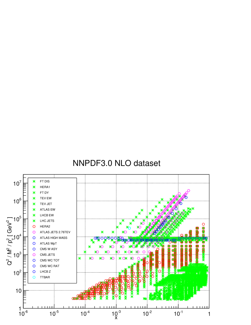
The kinematical coverage in the plane of the NNPDF3.0 dataset is shown in the scatter plot Fig. 1 (note that for hadronic data leading-order kinematics has been assumed for illustrative purposes, as discussed in [10]).
| Experiment | Dataset | Ref. | Sys. Unc. | no cuts | Kinematics | ||
| (NLO/NNLO cuts) | |||||||
| NMC | |||||||
| NMC | [19] | A | full | 211 (132/132) | |||
| NMC | [20] | A | full | 289 (224/224) | |||
| SLAC | |||||||
| SLAC | [23] | A | none | a | 191 (37/37) | ||
| SLAC | [23] | A | none | a | 191 (37/37) | ||
| BCDMS | |||||||
| BCDMS | [21] | A | full | b | 351 (333/333) | ||
| BCDMS | [22] | A | full | b | 254 (248/248) | ||
| CHORUS | |||||||
| CHORUS | [35] | A | full | c | 572 (431/431) | ||
| CHORUS | [35] | A | full | c | 572 (431/431) | ||
| NuTeV | |||||||
| NuTeV | [36, 37] | A | none | 45 (41/41) | |||
| NuTeV | [36, 37] | A | none | 44 (38/38) | |||
| HERA-I | |||||||
| HERA-I NC | [24] | M | full | d | 434 (379/379) | ||
| HERA-I NC | [24] | M | full | d | 145 (145/145) | ||
| HERA-I CC | [24] | M | full | d | 34 (34/34) | ||
| HERA-I CC | [24] | M | full | d | 34 (34/34) | ||
| ZEUS HERA-II | |||||||
| ZEUS-II NC | [33] | M | full | e | 90 (90/90) | ||
| ZEUS-II CC | [34] | M | full | e | 37 (37/37) | ||
| ZEUS-II NC | [53] | M | full | f | 90 (90/90) | ||
| GeV2 | |||||||
| ZEUS-II CC | [54] | M | full | f | 35 (35/35) | ||
| GeV2 | |||||||
| H1 HERA-II | |||||||
| H1-II NC | [51] | M | full | g | 139 (139/139) | ||
| GeV2 | |||||||
| H1-II NC | [51] | M | full | g | 138 (138/138) | ||
| GeV2 | |||||||
| H1-II CC | [51] | M | full | g | 29 (29/29) | ||
| GeV2 | |||||||
| H1-II CC | [51] | M | full | g | 29 (29/29) | ||
| GeV2 | |||||||
| H1-II low | [52] | M | full | 136 (124/124) | |||
| GeV2 | |||||||
| H1-II high | [52] | M | full | 55 (52/52) | |||
| GeV2 | |||||||
| HERA | [55] | M | full | 52 (47/47) | |||
| GeV2 | |||||||
| Experiment | Dataset | Ref. | Sys. Unc. | no cuts | Kinematics | ||
| (NLO/NNLO cuts) | |||||||
| DY E866 | |||||||
| DY E866 | [41] | M | none | 15 (15/15) | |||
| DY E866 | [39, 40] | M | none | 184 (184/184) | |||
| DY E605 | [38] | M | none | 119 (119/119) | |||
| CDF | |||||||
| CDF rap | [43] | M | full | h | 29 (29/29) | ||
| CDF Run-II jets | [83] | M | full | h | 76 (76/52) | ||
| D0 | |||||||
| D0 rap | [44] | M | full | 28 (28/28) | |||
| ATLAS | |||||||
| ATLAS 2010 | [47] | M | full | i | 30 (30/30) | ||
| ATLAS 7 TeV jets 2010 | [50] | M | full | i,j | 90 (90/9) | ||
| ATLAS 2.76 TeV jets | [63] | M | full | j | 59 (59/3) | GeV | |
| ATLAS high-mass DY | [56] | M | full | 11 (5/5) | GeV | ||
| ATLAS | [57] | M | full | 11 (9/-) | GeV | ||
| CMS | |||||||
| CMS electron asy | [48] | M | cov | 11 (11/11) | |||
| CMS muon asy | [58] | M | cov | 11 (11/11) | |||
| CMS jets 2011 | [62] | M | full | 133 (133/83) | GeV | ||
| CMS total | [60] | M | cov | 5 (5/5) | |||
| CMS ratio | [60] | M | cov | 5 (5/5) | |||
| CMS 2D DY 2011 | [59] | M | cov | 124 (88/110) | GeV | ||
| LHCb | |||||||
| LHCb rapidity | [49] | M | cov | 10 (10/10) | |||
| LHCb rapidity | [61] | M | cov | 9 (9/9) | |||
| ATLAS | [65, 66, 67] | M | none | 3 (3/3) | - | ||
| CMS | [68, 69, 70] | M | none | 3 (3/3) | - | ||
| Total | 5179 (4276/4078) | ||||||
| Experiment | Dataset | Ref. | Sys. Unc. | no cuts | Details |
| H1 | |||||
| H1 01 | [30] | full | 12 | Superseded by combination | |
| H1 09 | [31] | full | 6 | ” | |
| H1 10 | [32] | full | 26 | ” | |
| ZEUS | |||||
| ZEUS 99 | [26] | full | 21 | Superseded by combination | |
| ZEUS 03 | [27] | full | 31 | ” | |
| ZEUS 08 | [28] | full | 9 | ” | |
| ZEUS 09 | [29] | full | 8 | ” | |
| CDF | |||||
| CDF asymmetry | [42] | full | 13 | Lepton-level data from LHC | |
| D0 | |||||
| D0 Run II cone jets | [46] | full | 110 | Infrared unsafe at NNLO | |
cross section
2.2 New experimental data in NNPDF3.0
We now examine in more detail the features of the new experimental data that has been included in NNPDF3.0. We begin with the new deep-inelastic scattering data. In this work we have supplemented the combined HERA-I dataset with the inclusion of all the relevant HERA-II inclusive cross sections measurements from H1 and ZEUS [51, 52, 53, 54]. These data improve the statistical and systematic precision of medium- and high- data from the HERA-I run, and thus provide valuable information for quarks at medium and large . In addition, we have included low- data from H1 that provides additional information on the small- gluon and that could also be sensitive to potential deviations from fixed-order DGLAP at small-.
From the H1 experiment, we have included the new high- data from the HERA-II run [51], which covers the large region, GeV2, with improved statistical and systematic precision in comparison to Run-I. These data, taken at the default proton beam energy of GeV used in most of the HERA-II run, have been supplemented with inclusive cross-section measurements performed at lower center-of-mass energies [52], obtained with proton beam energies of GeV and GeV. These lower-energy measurements are the same ones used to determine the longitudinal structure function . Therefore, we exclude the previously used [25] data from the present fit to avoid any double counting, and for the same reason we do not include any other of the updated extractions at HERA [84, 85]. For completeness, in NNPDF3.0 we also include the the high-inelasticity data that H1 extracted from their Run II measurements [52].
From the ZEUS experiment, in NNPDF2.3 we already included some HERA-II data [33, 34], for neutral- and charged-current DIS with an electron beam. We now also include neutral- and charged-current cross sections with a positron beam [54, 53], which have been published since. As in the case of H1, ZEUS Run II inclusive cross-sections exhibit reduced statistical and systematic uncertainties when compared to Run I data in the medium and large region. For both H1 and ZEUS, we use the data averaged over lepton beam polarizations.
Turning to semi-inclusive measurements, in NNPDF3.0 we have replaced the separate charm structure function data from the H1 and ZEUS experiments [26, 27, 28, 29, 30, 31, 32] with the combined HERA charm production dataset [55], which provides data for the reduced cross-section (rather than structure function) and is based on a more extensive dataset; furthermore, the cross-calibration between common systematics implies that the combined data is more accurate than the separate inclusion of the individual measurements. The combined HERA charm production cross-sections offer a handle on the small- gluon [86], provide a unique testing ground for different treatments of heavy quark mass effects, and allow one to extract the running charm quark mass with competitive uncertainties [87, 88].
Concerning vector boson production at the LHC, NNPDF2.3 already included some data taken at 7 TeV, in particular the CMS electron asymmetry data from an integrated luminosity of 880 pb-1 [48], the ATLAS and rapidity distributions from the 2010 run [47] and the LHCb forward production data also from 2010 [49]. These datasets have now been supplemented with essentially all vector boson production data which have become available since.
From the ATLAS experiment, we include the high-mass Drell-Yan production data from the 2011 run [56], based on an integrated luminosity of 4.9 fb-1. These data, presented in terms of the invariant mass of the electron pairs produced at an invariant mass larger than the peak, which extends to TeV, can be used to constrain the large- antiquarks. In addition, it was shown in Ref. [89] that high-mass Drell-Yan at the LHC can be used to constrain the photon PDFs of the proton, and it was indeed used there to construct the NNPDF2.3QED PDF set. We also include now the ATLAS measurement of the boson transverse momentum distribution from the 2010 run of the LHC at 7 TeV [57], corresponding to an integrated luminosity of 31 pb-1. This data, unlike the 7 TeV ATLAS measurement of the boson transverse momentum distribution [90], is provided with all information on correlated uncertainties and has the potential to constrain the gluon and the light quark distributions in the medium- region [79].
From the CMS experiment, we include the muon asymmetry data based on the full statistics (5 fb-1) of the 7 TeV run [58], which have substantially reduced statistical and systematic uncertainties. We also include the double-differential distributions for Drell-Yan production from low dilepton masses (from GeV) to high dilepton masses (up to TeV) in bins of the dilepton invariant mass and rapidity, from the full 2011 dataset [59]. The CMS data for the production of charm quarks associated to bosons [60], which we also include, provide the absolute cross sections, differential on the lepton rapidity from the decay , as well as cross-section ratios also binned in . They are both included, as the former constrain the shape and overall normalization of the total strangeness at and the latter offer some handle on the strangeness asymmetry in the proton, . Data from this same process are available from the ATLAS Collaboration [91], but are given at the hadron level and thus cannot be directly included in our fit (though they could be included by for example estimating a hadron-to-parton correction factor using MadGraph5_aMC@NLO).
Finally, we include the LHCb rapidity distributions from the 2011 dataset [61], which are more precise than the previous data from the 2010 run. The forward kinematics of this data provide constraints on PDFs at smaller and larger values of than the vector boson production data from ATLAS and CMS. Further LHCb data from the 2011 run for boson rapidity distributions in the channel [92] and for low mass Drell-Yan production [93] are still preliminary.
Concerning inclusive jet production from ATLAS and CMS, we include the CMS inclusive jet production measurement at 7 TeV from the full 5 fb-1 dataset [62], which has been provided with the full experimental covariance matrix, and which supersedes previous inclusive jet measurements from CMS [94]. This data has a large kinematical coverage: for example, in the central rapidity region, the CMS data reaches up to jet transverse momenta of more than 2 TeV, thus constraining the large- quark and gluon PDFs [95, 96]. From ATLAS, we include the new inclusive cross-section measurement at TeV [63], which is provided with the full correlation matrix with the corresponding TeV measurement. Measuring the ratio of jet cross-sections at two different center of mass energies enhances the PDF sensitivity thanks to the partial cancellation of theoretical (missing higher order corrections) and experimental (jet energy scale) systematic uncertainties [73]. On the other hand no LHC dijet data are included [97], since it is notoriously difficult to achieve a good description of these measurements [95].
Finally, we include six independent measurements of the total top quark pair production cross-section from ATLAS and CMS, both at 7 TeV and at 8 TeV. These data provides information on the large- gluon PDF, complementary to that provided by inclusive jet production. At 7 TeV we include the measurements in the dilepton channel, based on 0.70 fb-1 integrated luminosity from ATLAS [65] and on 2.3 fb-1 from CMS [68] and the measurements performed using lepton+jets events from ATLAS [66] and CMS [69]. At 8 TeV we have included the dilepton channel measurement corresponding to an integrated luminosity of 2.4 fb-1 by CMS [98] and the ATLAS analysis of the lepton+jets final state in a dataset corresponding to an integrated luminosity of 5.8 fb-1 [67].
2.3 Theoretical treatment
NNPDF3.0 PDFs are provided at LO, NLO and NNLO in perturbative QCD. While for most of the observables included in the fit NNLO QCD corrections are known, some observables are known only up to NLO, while for others only partial contributions to the full NNLO corrections have been calculated. Specifically, NNLO corrections are not available for two datasets included in our fit: the vector boson transverse momentum distribution and the rapidity distribution (since there are no NNLO calculations for jets and heavy quarks). For the jet inclusive cross section, only the -channel has been recently computed at NNLO [99, 82], while for the full cross section only an approximate NNLO prediction based on threshold resummation is available [100]. For all other observables included in the fit the cross sections are known up to NNLO.
The theoretical predictions for DIS observables have been implemented in the FastKernel framework and thoroughly benchmarked [12, 101]. Drell-Yan cross sections, both for fixed target and for collider experiments, are computed at NNLO by using the local -factors computed according to the procedure described in Ref. [12]: we define -factors as the ratio of NNLO to NLO calculations for fixed NNLO PDFs, that is
| (1) |
where is the partonic cross section computed at either NNLO or NLO accuracy, and is the corresponding parton luminosity computed with a reference set of NNLO parton distributions. The tools used to compute the -factors are described in Sect. 2.3.1. For a detailed description of the procedure that we adopt to include a subset of the inclusive jet data in our analysis, see Sect. 2.3.2.
Given that electroweak corrections can be relevant in the large invariant mass region covered by some of the experimental data included in our fit (see Ref. [102] for an overview), we provide EW corrections for all LHC vector boson production data. To include these corrections in our NLO and NNLO calculation, we compute factors, , defined analogously to Eq. (1), with the NNLO computation substituted by the NLO+EW one, and using NLO parton luminosities on both numerator and denominator. All details on their computation and implementation are provided in Sect. 2.3.3. The QCD NNLO and EW –factors for LHC gauge boson production are listed in Appendix A.
In this work, we do not include all-order perturbative resummation of QCD corrections: these will be the object of a future separate study, possibly leading to the construction of dedicated resummed sets. Also, we do not include nuclear corrections, which are relevant for fixed-target deuterium DIS data, neutrino DIS data, and fixed-target Drell-Yan data, given the substantial uncertainties in their modeling and their moderate impact [103]. We will briefly assess the impact of this omission in Sect. 5.1.4.
The way our dataset is constructed, and in particular which data are included at various perturbative orders, is discussed in Sect. 2.4.1 below.
2.3.1 Computational tools
The inclusion of perturbative corrections to hadronic processes in PDF fits requires the fast computation of the relevant cross-sections. Several fast interfaces have been developed to this purpose, including APPLgrid [104], which provides an interface to MCFM [105, 106] and NLOjet++[107], and FastNLO [108, 109], also interfaced to NLOjet++. The MCgrid [110] package interfaces the Rivet [111] analysis package to APPLgrid, making use of the BlackHat/Sherpa [112] prescription for NLO reweighting.
Recently, a new fast interface has become available, namely aMCfast [113], a code which provides the complete automation of fast NLO QCD calculations for PDF fits, interfaced to MadGraph5_aMC@NLO [114], which in turn achieves the complete automation of the computations of tree-level and next-to-leading order cross sections and of their matching to parton shower simulations.
Such tools have been used extensively in the present analysis. For the 7 TeV CMS jet data, we have used the FastNLO calculation with central scales . For the 2.76 ATLAS jet data, we have used instead the APPLgrid calculation, which uses the same scale choices. For consistency, we use exactly the same settings of the calculation, including the central scales, as were used in the corresponding ATLAS 7 TeV inclusive jet analysis. The CDF Run II jets have also been computed using the FastNLO calculation with the same central scales as in the ATLAS and CMS case.
For electroweak vector boson production data, we have used the APPLgrid code interfaced to MCFM6.6 in all cases, with a consistent choice of electroweak parameters. We use the scheme, with GeV, GeV and GeV-2 set as input parameters and , derived from those. We turn off the Narrow-Width approximation. For all rapidity distributions, we set , with . For the distribution we set , while in the case of CMS double-differential distribution we set the scales to the central value of the invariant mass bin. The MCFM6.6 calculations have been cross-checked with independent calculations of DYNNLO [115, 116, 117, 118] and FEWZ3.1 [119, 120] at NLO, with the same settings, finding perfect agreement in all cases.
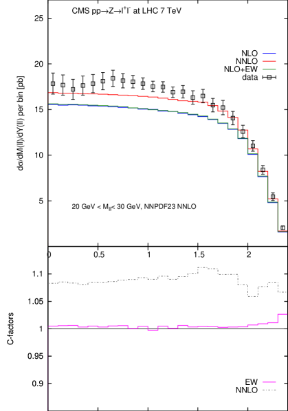
In the NNLO fits, the NNLO factors defined in Eq. (1) have been computed with FEWZ3.1 and cross-checked against DYNNLO1.3. Very high statistics runs of all these codes have been necessary to achieve negligible integration error in all the data bins. In order to obtain smooth -factors, the NNLO curves are smoothed with a high-degree polynomial interpolation. Notice that the difference between smoothed and original NNLO predictions is always within the Monte Carlo uncertainty of the code used to compute it. It turns out that these NNLO QCD corrections are sizable, especially for small invariant masses of the produced lepton pairs as it is shown on the right plot in Fig. 4: the NNLO -factor for the CMS double differential Drell-Yan data at low is around 10%, independent of the dilepton rapidity. NNLO corrections are also important for the ATLAS high-mass Drell-Yan data, reaching almost 10% around 1 TeV, see left plot of Fig. 4. Details of the computation of the EW corrections and their size are given below in Sect. 2.3.3.
For the computation of top quark pair production data at NLO, we again used APPLgrid interfaced to MCFM6.6. The NNLO factors have been computed by using the NNLO calculation of Ref. [81], as implemented in the top++ code [121]. Finally, we have used aMCfast interfaced to MadGraph5_aMC@NLO to compute the Higgs rapidity distributions in gluon fusion at NLO with an unphysical boson of mass GeV. As explained below in Sect. 3.2.1, this unphysical calculation has been used to enforce the positivity of cross-sections that depend on the small- gluon. More details about Higgs production at NLO in the MadGraph5_aMC@NLO framework can be found in in Refs. [122, 123].
2.3.2 Approximate NNLO treatment of jets
NNLO corrections to jet production in the the -channel have become available recently [99, 82]. An approximate NNLO prediction based on threshold resummation (but including all partonic subchannels) was presented in [100]. Its accuracy can now be gauged against the existing part of the full calculation.
This was done recently in a systematic study [124], to which we refer for a more detailed treatment. An important consequence of the analysis of Ref. [124] is that some of the comparisons between the exact computations and the threshold approximation performed hitherto [100] were marred by the fact that the renormalization scale was set equal to the jet transverse momentum in the threshold calculation, while the transverse momentum of the hardest jet was used instead for the exact calculation. It turns out that the perturbative expansion is rather better behaved, with smaller perturbative corrections, when the scale is used, and also, that the regions of agreement are rather different if a consistent scale choice is made: specifically, when using as a scale in the large rapidity region the accuracy of the threshold approximation appears to be very poor (while there is a better, accidental agreement when an inconsistent scale choice is made).
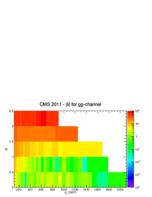
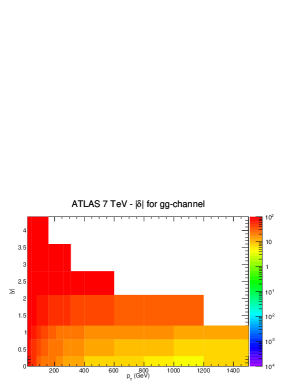
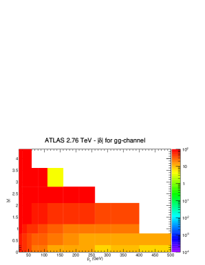
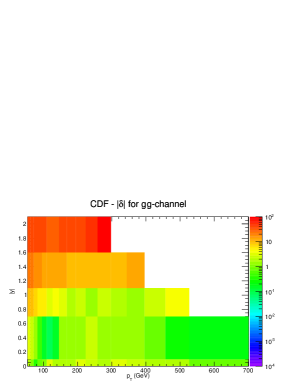
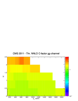
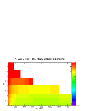
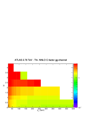
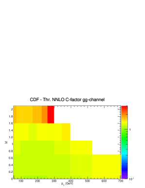
The percentage deviation between the exact and approximate calculation (with the renormalization scales set equal to in the two cases) is shown in Fig. 2 in the () plane for the CMS 2011 [62], ATLAS 7 and 2.76 TeV [50, 63] and CDF Run II [83] inclusive jet data included in our fit. A common NNLO reference PDF set, NNPDF2.3, is used in the two calculations. In Fig. 2, each of the entries of the contour plot correspond to one of the experimental data bins. It is apparent that the threshold approximation and the exact results are in reasonable agreement in the high- and central- regions. Note also that the disagreement between the two calculations can become very large for small transverse momenta and/or large rapidities.
In the kinematical region covered by the Tevatron and LHC jet cross-sections, see Fig. 2, the gluon channel is not necessarily dominant, however both theoretical arguments and the known NLO behavior suggest that the pattern of agreement or disagreement of the threshold and exact computations is similar in all partonic channels [124]. This result then suggests that the threshold approximation can be used provided all channels are included, and a sufficiently conservative cut is applied in order to keep only the regions in which the size of the deviation between the exact and threshold computations in the channel does not exceed a suitable low threshold.
Reassuringly, these are also the regions in which NNLO corrections are not too large, as it is apparent from Fig. 3, where we show the size of the approximate -factors. It is clear that the regions in which the quality of the approximation is better are the same as those where the size of the correction is relatively smaller, and conversely. In particular, in the region in which the exact and threshold NNLO calculations in the gluon channel differ by less than 10%, the -factor Eq. (1) (summing over all parton channels) is typically of order 15%, so the expected accuracy of the threshold approximation at NNLO is at the level of a few percent, smaller than the experimental uncertainties.
In NNPDF3.0, we thus follow the strategy of Ref. [124] and compute approximate NNLO -factors, Eq. (1), using the threshold calculation, while restricting the fitted dataset to the region where, thanks to the comparison with the exact calculation, we know the former to be reliable. This leads to the set of cuts outlined below in Sect. 2.4.
2.3.3 Electroweak corrections
Electroweak corrections, though generally small, may become large at high scales . While this will certainly be an issue for future LHC data at higher center of mass energy, already for some high-mass data included in our analysis the high accuracy of the experimental measurements may require theoretical predictions at the percent level of precision, and the size of the EW corrections needs to be carefully assessed.

The NLO EW one-loop corrections are known [125, 126, 127, 128, 129, 130] and have been implemented in several public codes such as HORACE [125] and ZGRAD2 [129, 130]. In FEWZ3.1 [119, 120] the NLO EW corrections are combined to the NNLO QCD corrections, using the complex mass scheme. This code allows the user to separate a gauge–invariant QED subset of the corrections from the full EW result. The QED subset includes initial–state QED radiation, final–state QED radiation (FSR) and the initial–final interference terms. The former cannot be consistently included without taking into account the photon PDF . Within the current uncertainties that affect the photon PDF, as determined in Ref. [89], initial–state QED corrections are compatible with zero for most of the data included in the analysis. In case they may be larger, we exclude the data from the fit, as explained in Sect. 2.4.1. As far as final state radiation (FSR) is concerned, when available, we use data from which it has already subtracted. These include all ATLAS and CMS electro-weak vector boson production data, which have been corrected for FSR (though the correction has not been applied to LHCb data).
We may thus consistently isolate and compute the weak component of the EW corrections with FEWZ3.1 and include it in our calculation via the computation of factors for all the electroweak gauge boson production. The size of the corrections is displayed in Fig. 4. We find that the effect of the pure EW corrections is negligible for most of the data in the Z peak region, of the order 1% or below. For the CMS double differential distributions, in the smallest invariant mass bin, we find that the pure EW corrections are small, much smaller than the NNLO QCD corrections. At large invariant masses the pure EW corrections are rather large and negative, as expected from the results of Ref. [131]. This can be clearly seen in Fig. 4 for the ATLAS high-mass Drell-Yan data, where EW corrections reach in the last bin of the distribution corresponding to a dilepton invariant mass of . Note that for the last bin of invariant mass measured by CMS, GeV, EW effects are still moderate, since due to the steep fall-off of the cross-section, most of the events are from the region around GeV.
In summary, although the ATLAS high mass distribution is the only measurement for which EW corrections are required, for consistency we include them for all the production data.
2.3.4 Treatment of heavy quarks
As in previous NNPDF analyses, in NNPDF3.0, heavy quark structure functions have been computed using the FONLL general-mass variable-flavor-number (GM-VFN) scheme [132]. In this scheme, the massive fixed-order calculation (in which the heavy quark is only counted in the final state) and resummed calculation (in which the heavy quark is treated as a massless parton) are consistently matched order by order. There is some latitude in deciding at which order the fixed-order massive result ought to be included when parton evolution is treated at a given perturbative order, and the FONLL method allows consistent matching in any case. Specifically, in a NLO computation one may decide to include massive contributions to structure functions up to , (on the grounds that this is the order at which the massless structure functions are also computed) or up to , (on the grounds that the massive structure function starts at ). These are called respectively FONLL-A and FONLL-B schemes [132]. At NNLO, while a similar ambiguity would exist in principle, in practice the massive coefficient function can only be included up to (FONLL-C) because the massive result is not known (progress in this direction is reported e.g. in [133])
While the FONLL-A scheme was used for the NNPDF2.1 and NNPDF2.3 NLO PDF sets, we now adopt the FONLL-B scheme for NNPDF3.0 NLO, with FONLL-C used at NNLO. While this scheme is less systematic, in that when going to NLO to NNLO the massless computation goes up one order but the massive one does not, it has the advantage that massive terms at NLO are more accurate, thereby allowing for the inclusion of a somewhat wider set of data already at NLO, as small- and charm production data are affected by large corrections, and cannot be described in the FONLL-A scheme. For the same reason, using FONLL-B allows for a more accurate description of the HERA inclusive cross section data at small-.
Heavy quark structure functions are computed using the expression which corresponds to the pole mass definition. Note that the distinction between pole and mass is only relevant at NNLO and beyond [134]. In this paper, we adopt the following values for the heavy quark pole masses,
| (2) |
which correspond to the current PDG values for the masses. Note that these values are different from the ones used in NNPDF2.3, namely GeV, GeV and GeV. A full discussion of heavy quark mass dependence will be the subject of future work; for the time being we have checked that the dependence of our results on the value of the heavy quark masses is moderate, in agreement with previous findings in the framework of NNPDF2.1 [11], as we shall briefly discuss in Sect. 5.1.4 below.
In NNPDF3.0 we take as a default the scheme, in which the number of active flavors never exceeds (i.e. in the fit the top quark is always treated as massive, never as a parton), though results will also be provided in the , and schemes. Note that in NNPDF2.1 and NNPDF2.3 the default was (with the other cases also provided). While in previous PDF determinations the distinction between and was relevant only for delivery, as no data above threshold were available, now several jet data (especially for 2011 CMS inclusive jets, which has the highest reach in ) are above top threshold, as well as some CMS and ATLAS high-mass Drell-Yan data. Close to top threshold use of an scheme might be advantageous because the top mass is treated exactly, while the loss of accuracy due to the fact that the running of differs from the exact running [135] is a comparatively smaller effect (only visible for processes which start at high order in , see e.g. [136]). Furthermore, most of the codes which we used for NNLO computations (specifically NLOjet++ and FEWZ) use an scheme, and the same is true for many of the codes and interfaces used in the computation of LHC processes. With an ever increasing set of LHC data, the use of an both in fitting, and as a default for PDF delivery appears thus to be more advantageous.
2.4 Construction of the dataset
We strive to include as much of the available experimental data as possible in our dataset. However, cuts have to be applied in order to ensure that only data for which the available perturbative treatment is adequate are included in the fit. These cuts are discussed in Sect. 2.4.1. Also, we include all available information on correlated uncertainties; however, there is some latitude in the treatment of correlated systematics, which we discuss in Sect. 2.4.2.
2.4.1 Kinematic cuts
As in previous NNPDF fits, we apply a cut in and to fixed-target DIS data, in order to make sure that higher-twist corrections are not needed:
| (3) |
The stability of the fit with respect to these choices (and in particular the explicit check that they eliminate the need for higher twists) has been studied in detail in Ref. [103]. Low-scale DIS data carry less weight in our current fit than they did previously, because of the inclusion of a large amount of new HERA and LHC data. Therefore, the impact of these choices is even less important than it was previously. Note that all NNPDF fits include target-mass corrections, followind the method of Ref. [6].
As discussed in Sect. 2.3 above, NNLO corrections are not available for the distribution and for production. As a consequence, ATLAS distribution data are included only in the NLO fit. However, we include the CMS distributions also in the NNLO fit, but with matrix elements computed up to NLO only (but running at NNLO) because these data almost only affect the strange distribution, and the uncertainty on strangeness is rather larger than the typical size of NNLO corrections, so we would rather keep the corresponding experimental information.
| Experiment | Exclusion regions in the () plane | ||
|---|---|---|---|
| CDF Run-II jets [83] | 52 | GeV, GeV | |
| all bins | |||
| ATLAS 2.76 TeV jets [63] | 3 | GeV | |
| all bins | |||
| ATLAS 7 TeV jets 2010 [50] | 9 | GeV | |
| GeV | |||
| all bins | |||
| CMS jets 2011 [62] | 83 | GeV | |
| all bins | |||
For inclusive jet production, we include all available data in the NLO fit, while in the NNLO fit we include only the data points such that the relative difference between the exact and the approximate -channel NNLO -factors differ by less than 10%. As already mentioned in Sect. 2.3.2 above, a cut on the size of the -factors, only accepting jet data for which the NNLO -factor does not exceed 15%, results in approximately the same dataset. In Tab. 4 we summarize the ensuing exclusion regions in the () plane and the number of data points points which survive the cut for each experiment. As discussed in Ref. [124] and Sect. 2.3.2 above, this choice of cut ensures that NNLO corrections are included with an expected accuracy of a few percent for all the bins in of the inclusive jet cross section data.
For the ATLAS measurement of the transverse momentum distribution, we include only those data points with GeV. This cut excludes the first two bins in , and is motivated by the observation that at small the perturbative series is not well-behaved and all-order resummation is needed (either analytically or by matching the fixed order calculation to a parton shower).
For the neutral-current Drell-Yan measurements from ATLAS and CMS, we include only data for which the dilepton invariant mass satisfies GeV. This excludes the last six bins of the ATLAS DY invariant mass distribution and the 12 points in the rapidity distribution corresponding to the last bin of invariant mass, GeV, for the CMS measurement. The reason behind this cut is that the pure weak corrections that we include in our calculation, using FEWZ, do not include the QED subset of the total electroweak correction. In particular, including the photon–initiated contributions to the dilepton cross-section would require an initial photon PDF , which is not fitted in this analysis. Using the NNPDF2.3QED set, we have found that, while for most data points this contribution is compatible with zero within the photon PDF uncertainty, for values of above such correction can become sizable, more than a few percent, and up to 20% for the highest invariant mass values. On this ground, we exclude all neutral-current Drell-Yan data with GeV from the fit, both at NLO and at NNLO.
The final cut is imposed, for the NLO fit only, to the lowest invariant-mass bin of the CMS Drell-Yan double differential distributions. As can be seen from Fig. 4 (right plot), for the bin with invariant mass GeV, the NNLO –factors are large, around 10%, while experimental uncertainties are a few percent. Therefore, it is not possible to obtain a reasonable fit to these data points in a NLO fit, and therefore the 24 points of the GeV bin of the CMS data are excluded from the NLO analysis.
The number of data points before and after cuts, both in the NLO and NNLO fit, are summarized in Tab. 3. At LO we use the same cuts as in the NLO fit: this is a sensible choice, given that theory uncertainties at LO are larger than experimental uncertainties, it does not make much sense to attempt to devise a set of optimized kinematical cuts specifically for the LO fits.
2.4.2 Treatment of correlated systematic uncertainties
In NNPDF3.0 we include all available information on correlated systematic uncertainties. This information is summarized in Tabs. 1 and 2. All experiments provide uncorrelated statistical uncertainties; and most of them also a correlated normalization uncertainty. The exception of the latter case are ratio experiments such as NMC , E866 and the CMS electron and muon asymmetries, and measurements which are normalized to the fiducial cross section like the D0 rapidity distribution, the ATLAS distribution and the CMS 2D Drell-Yan data. On top of these two types of uncertainties, most experiments also provide information on correlated systematics, either as an overall covariance matrix, or as a set of nuisance parameters with the corresponding correlation. The last case is the most complete in that each individual source of systematic uncertainty can be in principle treated independently.
In Tabs. 1 and 2 we indicate in the 5th column whether the information on correlated systematics, on top of the normalization, is either not provided, provided as a covariance matrix, or fully provided with a complete breakdown of all the sources of systematic uncertainties. Furthermore, in the 6th column, datasets which are affected by common correlated systematics are flagged with the same letter. In Tab. 1, all the DIS datasets that are labelled with the same letter in this column share a common normalization uncertainty. In addition, the BCDMS, CHORUS, HERA-I, ZEUS HERA-II and H1 HERA-II datasets share other correlated systematic uncertainties. In Tab. 2, the CDF datasets share a normalization uncertainty, the ATLAS 7 TeV jets and rapidity distributions also have a correlated normalization uncertainty, and the ATLAS inclusive jet measurements at 2.76 TeV and 7 TeV share a number of systematic uncertainties, most importantly the jet energy scale. On the other hand, none of the CMS datasets has common correlated uncertainties among them.
Normalization uncertainties are special because the uncertainty is proportional to the measured value, i.e. they are “multiplicative”. This poses peculiar problems in including them in a fit, because their naive inclusion in the covariance matrix would lead to a systematically biased result [137]. A full solution to this problem based on an iterative procedure (the method) has been presented in Ref. [9] and adopted by NNPDF in all PDF determination from NNPDF2.0 onwards (previous approximate solutions such as adopted in the MSTW08 [138] PDF determination lead in practice to very similar results in most realistic situations, see Refs. [139, 140]).
In hadron collider experiments, not only normalization uncertainties but most, or perhaps all other correlated sources of uncertainty are also multiplicative. After checking with the respective experimental collaborations, we have thus concluded that the most accurate treatment of correlated systematics is obtained by departing from the standard approach of fixed-target deep-inelastic experiments, in which all systematics but normalizations are additive [141], and treating all systematics as multiplicative for hadronic collisions. For deep-inelastic experiments, we treat all the correlated systematics of the HERA data as multiplicative, while for fixed-target experiments the systematics are treated as additive and only the normalization uncertainties as multiplicative. This information is also summarized in Tabs. 1 and 2, where in the 4th column experiments for which correlated systematic uncertainties are treated multiplicatively are denoted by M and others are denoted by A (additive uncertainties); normalization uncertainties are treated multiplicatively for all experiments. In Sect. 5 we will study the effect of a multiplicative vs. additive treatment of systematics, and find that it is small though perhaps not completely negligible. This will be especially true for the gluon PDF at large , which is determined from collider jet data, for which an accurate treatment of experimental systematics is crucial.
As usual in the NNPDF methodology, we use the information on correlated systematics both in order to calculate the used in fitting PDF to the Monte Carlo replicas, and also for generating the Monte Carlo replicas themselves. As explained in [6] (see also Eq. (21) in Sect. 4), the generation of the Monte Carlo replicas requires the knowledge of the individual sources of independent correlated systematic uncertainties. As can be seen from Tab. 2, for some LHC experiments this breakup is not provided and only the experimental covariance matrix is available. In those cases, we first create a set of artificial systematics consistent with the covariance matrix. These are obtained by diagonalizing the covariance matrix and then rescaling each eigenvector by the square root of its eigenvalue. This provides a set of artificial systematics which can be used to generate replica datasets in the same way as if we had the full breakup of systematics uncertainties, and which recombine correctly to give the original covariance matrix. This procedure effectively allows us to generate replica data according to the multivariate Gaussian distribution implied by the experimental covariance matrix.
3 Improved methodology
The inclusion of a substantial number of LHC
datasets in a global PDF determination presents a variety of technical
challenges, both in terms of the complexity of adding new hadronic observables
into the fitting machinery and of
the corresponding increase in the computational cost of
running fits.
The implementation of the enlarged LHC dataset is particularly demanding
for NNPDF, which, being based upon a genetic algorithm minimization in a large parameter
space, is already more computationally intensive than competing approaches.
To provide an optimized solution to these challenges, for NNPDF3.0
we have developed a brand new fitting code based on
C++ and Python, object-oriented languages that allow us
to streamline
the inclusion of new datasets and to achieve a highly efficient implementation
of the minimization algorithms.
In what follows we first describe the modifications of the fitting code which make it more robust and efficient. Then we discuss the new PDF parametrization and the enforced positivity constraints. Finally, we discuss the improvements in the minimization strategy.
3.1 Code
The majority of the computer time spent in performing a PDF fit arises from the calculation of the physical observables for the comparison with experimental data. Indeed, any PDF determination involves an iterative procedure where all the data points included in the fit need to be recomputed a very large number of times for different functional forms of the input PDFs. The computation of physical observables in the NNPDF framework is based upon the FastKernel method introduced in Refs. [10, 13]. We refer the reader to the original publications for a detailed explanation of the method; here we simply recall a few basic facts that are necessary to explain the structure of the new code.
3.1.1 FastKernel methodology
For a suitable choice of interpolating functions, the parton distributions at a given scale are represented on a grid of points in :
| (4) |
where the index identifies the parton flavor, and the index enumerates the points on the grid.
Deep-inelastic observables, which are linear in the PDFs, can be computed using a precomputed kernel :
| (5) |
The index here labels the physical observable, and are the corresponding kinematical variables for each particular experimental data point, runs over the points in the interpolating grid and is a parton flavor index. The kernel is referred to as an FK table. Similarly, hadronic observables, which are written as a convolution of two PDFs, can be computed in terms of an (hadronic) FK table ; the final expression is:
| (6) |
Once again we used the index to identify the physical observable and to label the specific experimental data point for this observable; the indices run over the parton flavors, and the indices count the points on the interpolating grids. In the fitting code, for each experimental dataset we will have a separate FK table that encodes all the theory information.
The quantities and in Eqs. (5, 6) encode all the information about the theoretical description of the observables e.g. the perturbative order, the value of the strong coupling, the choice of scales, the QCD and electroweak perturbative corrections, or the prescription for the evolution. A modification in the theoretical formulation is reflected in a new FK table. The convolutions of the FK tables with the PDFs at the initial scale are generic, and do not require any knowledge about the theoretical framework. It is thus clear from their structure that the FK tables now implement a clean separation of the theory assumptions from the actual fitting procedure. During a fit, the PDFs at the initial scale are varied in order to minimize the while the FK tables are always kept fixed and treated as an external input.
It should be emphasized that the main difference between fast NLO calculators such as FastNLO, APPLgrid and aMCfast, and our FastKernel method is that in the latter also the PDF evolution is included into the precomputed tables, while the other approaches require as input the PDFs evolved at the scales where experimental data is provided. This optimization step is essential to reduce the computational cost of running NNPDF fits. Note also that the generic structure Eqs. (5, 6) holds for any fast NLO calculator as well as for any PDF evolution code. In NNPDF3.0 we use our own internal Mellin-space Fkgenerator code for PDF evolution and DIS observables, but using -space codes such as HOPPET [142] or APFEL [101] should also be possible.
The fact that the expressions Eqs. (5, 6) of observables in terms of FK tables include the appropriate PDF evolution pre-computed in the FK tables (for DIS data) and (for hadronic observables) is particularly important for processes for which the precomputed fast NLO matrix elements, obtained for example from APPLgrid or FastNLO, require the PDFs at a large number of values. This is specially true for inclusive jet production, where for each experimental bin the range of values for which PDFs need to be provided is different (since this range depends on the jet and rapidity). In these cases, the associated acceleration due to the pre-computation of the PDF evolution makes all the difference between a process being practical or impossible to include in an NNPDF fit. The improvement due to this acceleration is quantified in Tab. 5 below.
3.1.2 NNPDF++
For the NNPDF3.0 determination, a new fitting toolchain has been developed
from scratch with the FK procedure at its core in order to ensure
that the most expensive part of any fit, the calculation of the physical observables,
is performed in the most efficient manner possible.
As discussed above the new fitting code has been designed
with an explicit separation between experiment and theory, with all theory
information contained within the FK tables,
and all experimental information held within a new data file format,
internally dubbed CommonData.
These two data formats have an associated class structure built in
modular C++ (which replaces the previous FORTRAN
implementation),
each retaining the following areas of jurisdiction:
-
•
Theoretical treatment: FK tables
-
–
PDF evolution.
-
–
NLO QCD hard-scattering matrix elements.
-
–
Perturbative order, value of / and values of the heavy quark masses.
-
–
Heavy flavour renormalization scheme.
-
–
NNLO QCD C-factors.
-
–
NLO electroweak C-factors.
-
–
-
•
Experimental information: CommonData
-
–
Process type information.
-
–
Experimental kinematics for each data point.
-
–
Experimental central values.
-
–
Full breakdown of experimental systematic uncertainties.
-
–
Flexible choice of additive/multiplicative for the treatment systematic uncertainties.
-
–
The inclusion of a new experimental dataset into an NNPDF fit is therefore now a matter of converting the experimental results into the CommonData file format, and generating a set of FK tables each with the desired choices of theory parameters. Once generated, the CommonData and FK files are stored, and accessed thereon only via a set of classes used universally throughout the NNPDF++ fitting code.
These new code structures have enabled a number of methodological improvements by providing a more efficient and flexible treatment of experimental data. For example, performing kinematic cuts upon an experimental dataset can now be performed simply and algorithmically by selecting the points in the CommonData format which pass the required cuts according to their bundled kinematic information, and matching with the equivalent points in the FK table. This is a considerable improvement over the earlier structure in FORTRAN whereby a variation of kinematical cuts necessitated a complete regeneration of the pre-computed theory tables due to the monolithic treatment of experimental data.
While the construction of this new fitting toolchain in C++ has made
it possible to streamline
any variation in the theory settings and experimental cuts, the new fitting
code itself also achieves substantial improvements over the previous FORTRAN
implementation.
A modular treatment of most of the fitting procedure has been implemented, including
PDF parametrization (both in terms of the flavor basis and of
the specific functional form), minimization methods and
stopping criteria.
This allows for the rapid and safe
replacement or improvement of separate modules of the NNPDF fitting
framework
without the need
for a large amount of programming work, enabling methodological studies
of a greater depth than those that we have been able to
perform previously, as we shall report in later sections.
To ensure a fast and efficient minimization procedure, the calculation of observables in the FK convolution (the main bottleneck here) has been carefully optimized. In particular, the FK class that holds the hadronic table from Eq. (6) has been designed such that the table is stored with the optimal alignment in machine memory for use with SIMD (Single Instruction Multiple Data) instructions, which allow for an acceleration of the observable calculation by performing multiple numerical operations simultaneously. The large size of a typical FK product makes the careful memory alignment of the FK table and PDFs extremely beneficial. A number of SIMD instruction sets are available depending on the individual processor. By default we use a 16-byte memory alignment for suitability with Streaming SIMD Extensions (SSE) instructions, although this can be modified by a parameter to 32-bytes for use with processors enabled with Advanced Vector Extensions (AVX). The product itself is performed both with SIMD instructions and, where available, OpenMP is used to provide acceleration using multiple CPU cores. An implementation of the FK product for GPUs, while presenting no technical objections, has so far not been developed due to scalability concerns on available computing clusters.
Thanks to the implementation of these various conceptual and technical optimizations in the calculation of physical observables, the NNPDF3.0 fitting code benefits from a substantial speed-up with respect to alternative calculations, using for example APPLgrid, where the PDF evolution needs to be performed separately from the calculation of hard-scattering matrix elements. This performance improvement is also clearly visible when comparing with the calculation of the hadronic convolution Eq. (6) using the optimized settings with that using non-optimized settings. To illustrate this point, in Tab. 5 we compare the timings, for a couple of representative LHC observables, for the convolution performed using APPLgrid, a naive FK implementation, and the optimized FK implementation using the SSE-accelerated calculation, for two representative observables. From Tab. 5 it is clear that a massive improvement in speed is achieved by precomputing the PDF evolution in the FK table, with further improvements obtained by the careful optimization of the FK product, and even further gains possible when combined with OpenMP on a multiprocessor platform.
| Observable | APPLgrid | FK | optimized FK |
|---|---|---|---|
| production | 1.03 ms | 0.41 ms (2.5x) | 0.32 ms (3.2x) |
| Inclusive jet production | 2.45 ms | 20.1 s (120x) | 6.57 s (370x) |
3.2 PDF parametrization
As compared to the NNPDF2.3 analysis, there have been a number of substantial modifications in the way PDFs are parametrized and constrained. These include the choice of input scale, the parametrization basis, preprocessing, and the implementation of PDF positivity, which we now discuss in turn.
3.2.1 Parametrization basis
In previous NNPDF fits, PDFs were parametrized at a reference scale = 2 GeV2. In NNPDF3.0 instead we choose = 1 GeV2. Of course, this choice has no effect whatsoever on the results of the fit: indeed, changing the input scale amounts to a change in the input PDF parametrization, of which our fits are fully independent, as we have checked at length previously, and will verify again here (see in particular Sects. 4.5.3, 4.5.4, 5.3.5). The motivation for lowering is to be able to span a wider range of possible values of the charm quark mass, without having to cross the initial evolution scale (i.e. while always having ), which will simplify future studies of heavy quark mass dependence.
At this reference scale, in previous NNPDF fits, including NNPDF2.3, PDFs were expressed in terms of the following set of basis functions for quark and antiquark PDFs:
| (7) | |||||
and then the gluon PDF . This basis was chosen because it directly relates physical observables to PDFs, by making the leading order expression of some physical observables in terms of the basis functions particularly simple: for example, is directly related to the difference in proton and deuteron deep-inelastic structure functions , and is simply expressed in terms of Drell-Yan production in proton-proton and proton-deuteron collisions, for which there is data for example from the E866 experiment.
With the widening of the experimental dataset in NNPDF3.0, there is little reason to favor any particular PDF combination based on data, and thus we prefer to choose the basis that diagonalizes the DGLAP evolution equations. We emphasize that the only purpose of such choices is to speed up the minimization while leaving results unaffected: independence of our results of this basis change will be checked explicitly in Sects. 4.5.3 and 5 below. The default basis in the NNPDF3.0 fits is thus
| (8) | |||||
and of course the gluon. Here, as in previous NNPDF fits, we do not introduce an independent parametrization for the charm and anticharm PDFs (intrinsic charm). However we do plan to do it in the near future.
As in all previous NNPDF fits, each basis PDF at the reference scale is parametrized in terms of a neural network (specifically a multi-layer feed-forward perceptron) times a preprocessing factor:
| (9) |
where is an overall normalization constant, and and denote the normalized and un-normalized PDF respectively. The preprocessing term is simply there to speed up the minimization, without biasing the fit. We now discuss the overall normalizations , while the preprocessing will be addressed in Sect. 3.2.2 below.
Out of the seven normalization constants, in Eq. (9), three can be constrained by the valence sum rules (for up, down and strange quarks) and another by the momentum sum rule. Which particular combinations depends of course of the choice of basis. With the default NNPDF3.0 basis, Eq. (8), these constraints lead to
| (10) | |||
The other normalization constants can be set arbitrarily to unity, that is : the overall size of these PDFs is then determined by the size of the fitted network. The finiteness of sum rule integrals Eq. (10) is enforced by discarding during the genetic algorithm minimization (see Sect. 3.3.1 below) any mutation for which the integrals would diverge. This condition, in particular, takes care of those NN configurations that lead to a too singular behavior at small-.
Thanks to the flexibility of the
new C++ fitting code, in NNPDF3.0 we support the option of using any
arbitrary basis for the neural network parametrization of PDFs.
This will allow us in
particular to check explicitly basis independence.
However, whenever
we use a basis which differs from
the evolution basis Eq. (8), the PDFs will be
transformed back to the evolution basis before preprocessing and
normalization are applied.
This has the advantage of ensuring that the
finite integrals Eq. (10) do not have to be constructed
as the difference of divergent integrals, which would require large
numerical cancellations, thereby potentially leading to numerical
instabilities.
3.2.2 Effective preprocessing exponents
As mentioned, when parametrizing PDFs in terms of neural networks, Eq. (9), preprocessing is introduced as a means to speed up the minimization, by absorbing in a prefactor the bulk of the fitted behaviour so that the neural net only has to fit deviations from it. However, we must make sure that the choice of preprocessing function does not bias the result. As in previous NNPDF fits, starting with NNPDF1.2 [8] onwards, this is done by randomizing the preprocessing exponents, i.e. by choosing a different value for each replica within a suitable range. Unlike in previous NNPDF fits, where this range was determined based on a stability analysis of the results, we now determine the range self-consistently in a completely automatic way (the same methodology was already used in the NNPDFpol family of polarized PDF determinations [143, 144]).
This is done in the following way. First of all, we define effective asymptotic exponents as follows:
| (11) | ||||
| (12) |
Other definitions would be possible, such as
| (13) |
We have checked that their use would not modify qualitatively our results. We choose a wide starting range for the preprocessing exponents for each PDF, and perform a fit. The effective exponents Eq. (11-12) are then computed for all replicas at and for the low- exponent and at and for the large- exponent , for all PDFs (except for the gluon and singlet small- exponent, , which is computed at ). The fit is then repeated by taking as new range for each exponent the envelope of twice the 68% confidence interval for each value. The process is then iterated until convergence, i.e., until the output preprocessing exponents stop changing. Reassuringly, convergence is typically very fast: even in the cases where the fitted dataset is varied significantly, only one iteration is needed to achieve stability.
This procedure ensures that the final effective exponents are well within the range of variation both in the region of the smallest and largest data points, and in the asymptotic region (these two regions coincide for the gluon and singlet at small ), thereby ensuring that the allowed range of effective exponents is not artificially reduced by the preprocessing, either asymptotically or sub-asymptotically.
The final output values of the preprocessing exponents for the central NLO and NNLO NNPDF3.0 fits are listed in Tab. 6. These ranges have been redetermined self-consistently for different fits: for example, for fits to reduced datasets, wider ranges are obtained due to the experimental information being less contraining.
| NLO | NNLO | |||
|---|---|---|---|---|
| [] | [] | [] | [] | |
| [1.06, 1.22] | [1.31, 2.68] | [1.02, 1.33] | [1.31, 2.74] | |
| [0.96, 1.37] | [0.28, 5.45] | [1.05, 1.53] | [0.85, 5.20] | |
| [0.54, 0.70] | [1.20, 2.91] | [0.54, 0.70] | [1.18, 2.80] | |
| [0.29, 0.58] | [1.31, 3.42] | [0.29, 0.61] | [1.36, 3.73] | |
| [0.54, 0.73] | [0.80, 3.09] | [0.55, 0.72] | [1.06, 3.07] | |
| [-0.17, 1.36] | [1.58, 3.14] | [-0.25, 1.41] | [1.64, 3.20] | |
| [0.54, 1.25] | [1.30, 3.42] | [0.54, 1.27] | [1.33, 3.23] | |
3.2.3 Positivity constraints
As is well known [145], beyond leading-order parton distributions do not need to be positive definite. However, the requirement that measurable physical observables be positive still imposes a generalized positivity constraint on the PDFs. In previous NNPDF fits these constraints were enforced by imposing positivity of the deep-inelastic structure functions , and of the neutrino charm production (“dimuon”) cross-section at a scale of GeV2 in the range (see in particular Sect. 4.5 and 5.5 of Ref. [10]). However, while these conditions were sufficient to guarantee the positivity of most physical observables in previous NNPDF fits, in order to ensure positivity of all observables, the number of independent positivity constraints must be at least equal to the number of independently parametrized PDFs.
In order to guarantee full positivity of physical observables we have thus enlarged the set of positivity constraints. In particular, we have chosen to impose positivity of some pseudo-observables which must respect positivity for reasons of principle, but which are not measurable in practice. We choose the three tagged deep-inelastic structure functions , and , and the three flavor Drell-Yan rapidity distributions, , and , defined respectively as the contribution to the structure function or the Drell-Yan rapidity distribution which is obtained when all quark electric charges are set to zero except that of the up, down or strange quark flavor, respectively. These six constraints enforce generalized positivity of the quark and antiquark PDFs. As in previous fits, our positivity conditions are imposed at the low scale of GeV2, and will then be also satisfied once the PDFs are evolved upwards in .
Generalized positivity of the gluon is enforced by requiring positivity of the light component of the longitudinal structure function , defined as the contribution to the structure function when all quark electric charges are set to zero but those of the three lightest flavors. The use of allows us to impose gluon positivity without having to make specific choices for the treatment of heavy quarks at the low scale where these conditions are imposed. This constraint is supplemented with that from the rapidity distribution for the production in gluon-gluon fusion of a Higgs-like scalar with mass GeV2 (such a constraint being much more stringent than that from prodiuction of a heavier Higgs). The use of these two observables ensures positivity of the gluon PDF both at small and at large values.
In summary, the pseudo-observables used to enforce generalized PDF positivity, expressed schematically in terms of their underlying parton content, the following:
| (14) | |||||
All these positivity constraints are imposed at GeV2, and for , which, because of the structure of QCD evolution, ensures positivity at all higher scales (and explains our choice for the mass of the Higgs-like scalar). In practice we compute the observables at 20 points in the given range, equally spaced on a log scale for (ten points) and on a linear scale for .
During the minimization, the positivity constraints are imposed by adding a Lagrange multiplier, and then further discarding replicas for which any of the pseudo-observables is negative by more than 25% of its absolute value computed with a fixed reference PDF set (typically, the outcome of a previous fit). The latter condition is necessary for cross sections which are very close to zero (e.g. close to kinematic boundaries, like the rapidity tails of Drell-Yan distributions) where the Lagrange multiplier strategy is not effective. For DIS structure functions and Drell-Yan distributions, the pseudo-observables are computed using the internal NNPDF FastKernel implementation, while the Higgs-like scalar production cross section is computed using MadGraph5_aMC@NLO [114] interfaced to aMCfast [113], using a tailored model which goes beyond the effective theory approximation for top quark mass effects [123, 146].
The strategy outlined above has been used to enforce generalized positivity both in the NLO and NNLO fits. The only difference is that in the NNLO fit we compute the pseudo-observables at NLO (with the PDFs evolved also at NLO for consistency) because at the low values at which the positivity pseudo-observables are computed, large unresummed NNLO corrections lead to perturbatively unstable predictions at large and small . In addition, there is some evidence that the resummed result is closer to NLO than to NNLO, see for example Ref. [147] for the case of deep-inelastic structure functions. The impact of the positivity constraints on the final PDFs is quite substantial, especially in the extrapolation regions, as one could expect. This statement will be quantified and discussed in Sect. 5.3, where we will compare two NNPDF3.0 NLO fits with and without the positivity constraints, and we will discuss further a posteriori checks of the implementation of the positivity conditions. In the results section, we also explore the impact of the improved positivity constraints on searches for high-mass new physics.
In the leading order fits, where PDFs should be strictly positive-definite, exactly the same strategy as in the NLO and NNLO fits is used (with pseudo-observables now computed at LO): we have verified that, as one could expect, using the conditions Eq. (14) expressed at LO leads to effectively positive-definite PDFs. To avoid the problem of the occasional replica of the LO fit that might become slightly negative, the LHAPDF6 NNPDF3.0LO grids provide by construction a positive-definite output. We have verified the robustness of our LO positivity implementation by comparing it to alternative strategies, such as using a neural network where the output of the last layer is squared.
3.3 Minimization algorithm
As in previous NNPDF fits, minimization is performed using genetic algorithms, which are especially suitable for dealing with very large parameter spaces. Because of the extreme flexibility of the fitting functions and the large number of parameters, the optimal fit is not necessarily the absolute minimum of the (see in particular the discussion in Sect. 4 of Ref. [6]), which might correspond to an ‘overfit’ in which not only the desired best fit is reproduced, but also statistical fluctuation about it. As a consequence, a stopping criterion is needed on top of the minimization method. In NNPDF3.0 we have improved both the minimization strategy and the stopping criterion.
3.3.1 Genetic Algorithms
We have performed a comprehensive re-examination of the genetic algorithm minimization procedure utilized in previous NNPDF determinations. Our approach has been to take a minimal starting methodology with only a few basic features. New features were added in turn and only retained if they resulted in faster fitting.
The algorithm consists of three main steps: mutation, evaluation and selection. Firstly, a large number of mutant PDF sets are generated based on a parent set from the previous generation. The goodness of fit to the data for each mutant is then calculated. The best fit mutant is identified and passed on to the next generation, while the rest are discarded. The algorithm is then iterated until a set of stopping criteria are satisfied.
The number of mutants tested each generation is now set to 80 for all generations, removing the two GA ‘epochs’ used in previous determinations. However, this number is somewhat arbitrary, as the more significant quantity in terms of fit quality is the total number of mutants produced during the fit, i.e. the number of mutants multiplied by the number of generations. If one is increased while the other is decreased by the same factor the fit results are largely unchanged. All mutants are generated from the single best mutant from the previous generation.
To generate each mutant, the weights of the neural networks from the parent PDF set are altered by mutations. In previous NNPDF fits the mutations have consisted of point changes, where individual weights or thresholds in the networks were mutated at random. However, investigations of strategies for training neural networks [148] have found that employing coherent mutations across the whole network architecture instead leads to improved fitting performance. The general principle that explains this is that of changing multiple weights which are related by the structure of the network, leading to improvements in both the speed and quality of the training.
The neural networks used in NNPDF fits consist of connected nodes organized in layers. To get a value from the network, the nodes in the input layer are set with the required and value and then the activations of nodes in successive layers are calculated according to
| (15) | ||||
| (16) |
where is the activation of the th node in the -th layer of the network, are the weights from that node to the nodes in the previous layer and is the threshold for that node. The weights and the thresholds are the parameters in the fit, and so are the objects which are changed in the mutation. The exception to Eq. (16) is the last layer, where in order to allow for an unbounded output a linear activation function is used instead. The flexibility of the fitting code allows us to easily explore other choices, for instance a quadratic output of the last layer, , has been used in studies of the PDF positivity in leading order fits.
In the NNPDF3.0 fits we use a nodal mutation algorithm, which gives for each node in each network an independent probability of being mutated. If a node is selected, its threshold and all of the weights are mutated according to
| (17) |
where is the baseline mutation size, is a uniform random number between and , different for each weight, is the number of generations elapsed and is a second uniform random number between and shared by all of the weights. An investigation performed on closure test fits found that the best value for is 15, while for the mutation probability the optimal value turns out to be around 5%, which corresponds to an average of 3.15 nodal mutations per mutant PDF set.
As with the removal of the fast- and slow-epochs and their replacement with a single set of GA parameters, the Targeted Weighted Training (TWT) procedure adopted in previous fits has also been dropped. This was originally introduced in order to avoid imbalanced training between datasets. With the considerably larger dataset of NNPDF3.0 along with numerous methodological improvements, such an imbalance is no longer observed even in fits without weighted training. Whereas previously the minimization was initiated with a TWT epoch in which the fit quality to individual datasets was minimized neglecting their cross-correlations, in NNPDF3.0 the minimization always includes all available cross-correlations between experimental datasets.
With the removal of the TWT mechanism, along with the consolidation of GA training into a single epoch with a unified set of mutation probabilities and sizes, the number of free parameters in the NNPDF minimization has been considerably reduced. In Tab. 7 we provide a comparison summarizing the relevant parameters in the NNPDF2.3 and NNPDF3.0 determinations.
| NNPDF 2.3 | 2500 | 50000 | 2.3 | 80 | 30 | |
|---|---|---|---|---|---|---|
| NNPDF 3.0 | - | 30000 | - | 80 | - |
| NNPDF2.3 | ||
| Single Parameter Mutation | ||
| 2 | 10, 1 | |
| 3 | 10, 3, 0.4 | |
| 2 | 1, 0.1 | |
| 3 | 8, 1, 0.1 | |
| 3 | 5, 1, 0.1 | |
| 2 | 5, 0.5 | |
| 2 | 1, 0.1 | |
| NNPDF3.0 | ||
|---|---|---|
| Nodal Mutation | ||
| 5% per node | 15 | |
| 5% per node | 15 | |
| 5% per node | 15 | |
| 5% per node | 15 | |
| 5% per node | 15 | |
| 5% per node | 15 | |
| 5% per node | 15 | |
3.3.2 Stopping criterion
As in previous NNPDF fits, the optimal fit is determined using a cross-validation method. This is based on the idea of separating the data in two sets, a training set, which is fitted, and a validation set, which is not fitted. The genetic algorithm is used in order to minimize the (or other figure of merit) of the training set, while the of the validation set is monitored along the minimization, and the optimal fit is achieved when the validation stops improving (see Ref. [6] for a more detailed discussion).
In previous NNPDF fits this stopping criterion was implemented by monitoring a moving average of the training and validation , and stopping when the validation moving average increased while the training moving average decreased by an amount which exceeded suitably chosen threshold values. The use of a moving average and of threshold values was necessary in order to prevent the fit from stopping due to a statistical fluctuation, but introduced a certain arbitrariness since the value of these three parameters (the length of the moving average and the two thresholds) had to be tuned.
In NNPDF3.0 we have improved on this: we now simply stop all fits at the point in which the fit reaches the absolute minimum of the validation within the maximum number of generations . In practice this is done in the following way. All replicas are minimized for generations. In the beginning of the fit, both the validation and the PDF configurations are stored. At the end of the each generation, the validation is computed again, and if it is lower than the previous stored values, the PDFs are replaced with the current ones, if not the fit proceeds to the next iteration. At the end, the stored PDFs have the the lowest validation seen during the fit, and they are taken as the global best fit. We call this the ’look-back’ method, and it is clearly completely objective. The price to pay for this is that now all replicas have to be run up to .
In order for the look-back method to be effective, the value of must be large enough that the PDFs at the minimum do not depend on it, i.e., such that the choice of a larger value does not lead to a different minimum. We have verified this explicitly by checking that results are unchanged if the value of is increased, see Sect. 4.5.1 below. We have furthermore checked that results are stable upon small variations of the position of the minimum: this guarantees that the choice of the absolute minimum (which could correspond to a local fluctuation) does not bias the result in any way. For this purpose, we have changed the look-back algorithm, by only updating the PDFs when the decreases by more than some threshold: we tried increasingly large threshold values (0.1, 1, and 10 on the total not divided by the number of data points) and verified that even though, of course, the stopping point changes, and happens at an earlier stage for large values of the threshold, the resulting PDFs are indistinguishable. This explicitly verifies that local minima whose validation values differ from the absolute minimum by a small amount correspond to essentially the same PDFs, as one might expect.
Even so, there is still the possibility that occasionally for a particular replica the training length required to reach the global minimum would be exceptionally long, either because of an unusual fluctuation of the pseudodata, or because of fluctuations in the minimization. In that case, the look-back method would not be effective, because the best within the maximal training length would still be far from the absolute minimum. In order to safeguard against this possibility, we consider the PDF arc-length defined as
| (18) |
suitably discretised. Use of an the arc-length penalty has been previously suggested as a way of penalizing functional forms that are too wiggly, see e.g. example the studies in Ref. [149].
We then take the value of as an indicator of convergence: a PDF replica with a very unlikely value of is assumed not to have converged, and thus discarded. This is implemented through an arc-length veto. The arc-length is computed for each PDF replica, and the average length and its standard deviation over the replica sample are determined for each PDF. We then discard PDF replicas for which at least one PDF the arc-length exceeds by more than four sigma the mean arc-length for that PDF.
Finally, at the end of the minimization, an a posteriori quality check on the resulting sample of Monte Carlo replicas is performed for each fit. These quality tests verify that the PDF generalized positivity has been successfully implemented (see discussion in Sect. 3.2.3), that no replica has a too unlikely arc-length, Eq. (18), and that likewise no replica has a too unlikely value of the . As in the case of arc-length, if any given replica has a whose value is more that four-sigma away the mean , it is automatically replaced by another replica that instead satisfies this condition.
4 Closure testing
In this section we describe in detail the strategy that has been used to validate the new fitting methodology described in the previous section: closure testing. The benchmarking of fitting methodology is especially important due to the substantial increase in experimental data included in NNPDF3.0, and the increased precision of the resulting PDFs: as data become more precise and their kinematic coverage increases, it becomes more and more important to eliminate methodological uncertainties, so that the only uncertainties in our PDFs are experimental and theoretical. For example a basic requirement for a successful methodology is to be able to fit widely different datasets with the same methodology, and without having to tune it or modify it according to the dataset, or to the theory which is used to describe it (for example at different orders in perturbative QCD). As we will show below, these requirements can indeed be achieved in the NNPDF3.0 framework. NNPDF3.0 is in fact the first PDF determination for which the complete fitting methodology has been thoroughly tested and tuned in closure tests based on pseudo-data that have the same kinematical coverage and statistical properties as the experimental data included in the fit. The idea of using perfect pseudo-data to validate some specific aspects of a PDF fitting methodology has been previously explored in Ref. [14].
The basic idea of the closure test is simple [2]: we take a given assumed form for the PDFs (for example MSTW08), a given theoretical model (for example NLO pQCD), and with them generate a set of global pseudo-data with known but realistic statistical properties (by using the covariance matrices of the real datasets that together make up, for example, the NNPDF3.0 dataset). These pseudo-data are then ‘perfect’, in the sense that they have known statistical properties, no internal inconsistencies, and are also entirely consistent with the theoretical model used to produce them. Thus if we then use our fitting methodology to perform a fit to these pseudo-data, we should reproduce the assumed underlying PDF, within the correct uncertainties. This latter point can be explored in some depth by changing by hand the level of uncertainties incorporated within the pseudo-data.
We will first introduce the idea of closure testing in the context of the NNPDF fits, and discuss its practical implementation. Then we will quantify the efficiency of our neural network training methodology by performing closure tests to perfect pseudo-data, without any fluctuations, so that the fit quality can be arbitrarily good. We then perform fits where the pseudo-data is supplemented with different levels of statistical and systematic fluctuations. Finally, in the last part of this section we use closure tests to assess the robustness of our methodology against variations of some of its ingredients, like the choice of PDF fitting basis or the dependence on the size of the neural network. Some of these last checks have also been performed on real data, as will be reported in Sect. 5.
4.1 NNPDF closure testing
The framework used in NNPDF3.0 for the computation of observables, as presented in Sect. 3.1.1, provides us with the ideal tool to successfully implement closure tests. In particular, the clean separation between theoretical assumptions and input PDFs allows us to generate pseudo-data using a given set of PDFs and the experimental covariance matrix as an input, and to perform a fit to this pseudo-data using exactly the same theoretical settings (encoded in the FK tables) that were used for generating them.
Throughout this section we shall refer to the parton distributions used to generate the pseudo-data as the input PDFs, and denote them by . Any PDF set available through the LHAPDF interface can be used as an input set to generate the pseudo-data: most of the closure tests described here will be performed using MSTW08, though we will also later describe results using other input PDFs. We denote the set of pseudo-data by : the dependence of the pseudo-data on the input PDF and experimental covariance matrix will be left implicit.
The outcome of the closure test fits is then a set of fitted PDFs, , which we will compare to the input PDFs in order to study the statistical precision and possible systematic biases in the fitting methodology. For any PDF set , whether input or fitted, the FastKernel framework delivers a set of theoretical predictions, , based on a particular theoretical model, which for present purposes we take to be NLO perturbative QCD, precisely as implemented in the NNPDF3.0 fits to real data, with the same parameter choices and so on. The one exception to this statement is that for closure tests to MSTW08 we drop the generalized positivity constraints introduced in Sect. 3.2.3, since positivity was imposed differently by MSTW. We have checked however, by performing closure tests based on NNPDF3.0 as input PDFs, that none of the conclusions drawn in this section is affected once the generalized positivity is included in the fit.
Fitting is performed by minimizing a function (denoted during the fitting as the ‘error function’): this is also used to assess the quality of the resulting fit. Such a depends on the dataset, , and on the theoretical predictions of the PDFs being fitted, :
| (19) |
In this expression, is the covariance matrix of the data (here we always use the -covariance matrix in order to avoid bias in the inclusion of multiplicative uncertainties, see Sect. 2.4.2), and is the total number of data points of the dataset. Note that when fitting the pseudo-data we thus use exactly the same procedure (in fact the same code) as we use in a fit to real data: we use the same error function, evaluated with the real data replaced by pseudo-data, the covariance matrix, and then the same fitting methodology (genetic algorithm, stopping criterion, etc). Since in the closure test fits the “correct” solution is known – it is given by the PDFs used as an input – the result of the fit should then reproduce the input PDFs within the statistical uncertainties of as determined by the fit.
For the purposes of the studies that will be performed in this paper, we will introduce three distinct categories (levels) of closure tests depending on the amount of stochastic noise added to the pseudo-data points generated from the initial PDFs. In order to make these tests as realistic as possible, this stochastic noise is generated using the complete information in the experimental covariance matrix, so that the fluctuations and correlations of the pseudo-data reproduce precisely those of the real experimental data. For the baseline closure tests presented in this section, the pseudo-data is in one-to-one correspondence with the experimental data used in the global fit, that is we have generated pseudo-data for every point in the NNPDF3.0 global dataset described in Tabs. 1 and 2.
The three levels of closure test that we will study, which we call Level 0, Level 1 and Level 2 for reasons that will soon become apparent, are set up as follows:
-
•
Level 0.
Using a given set of input PDFs, pseudo-data are generated using the FastKernel convolution, Eqs. (5,6). In these Level 0 fits, no stochastic noise is added to the pseudo-data. Then we perform fits, each to exactly the same set of pseudo-data, minimizing the error function (which here is the same as the per degree of freedom, i.e. ), but using different seeds for the initialization of the random numbers used in the minimization. This yields an ensemble of PDF replicas , where .
Note that the error function which we minimize is still computed using the covariance matrix of the data, even though now the pseudo-data have zero uncertainty. While of course the overall normalization of the error function is immaterial (as the minimum is at zero), this has the advantage of reproducing the correlations in the underlying dataset, which means that the total amount of independent experimental information (the number of independent data points) is the same as in the original dataset.
It should be clear from its definition that in Level 0 closure tests, the fit quality can be arbitrarily good, provided we use a sufficiently flexible PDF parametrization and a sufficiently efficient minimization algorithm. Indeed, since, by construction, the pseudo-data does not have any stochastic noise, and there are no inconsistencies, there exist perfect fits to the Level 0 pseudo-data that have a vanishing . We use the plural here because there clearly exists an infinity of fits which lead to vanishing by going through all data points, but differ in the way they interpolate between data points. These optimal solutions to the minimization problem reproduce precisely the predictions of the set of PDFs used as input in the generation of the pseudo-data at each of the experimental data points. The Level 0 closure test is thus a highly non-trivial test of the efficiency of the minimization procedure: at Level 0 the value of the error function (i.e., the evaluated for each replica) should decrease monotonically towards zero as the fit proceeds, if the functional form used for parametrizing the fitted PDFs is flexible enough. Consequently, the best-fit (i.e. the evaluated for the average of all replicas) should also go to zero.
-
•
Level 1.
Now we add stochastic fluctuations on top of the pseudo-data generated for the Level 0 closure tests, , as follows:
(20) where, as explained in [6], , and are the statistic, systematic and normalization uncertainties for each dataset, and the random numbers , and are generated with the appropriate distribution to reproduce the experimental covariance matrix. These shifted data points represent the central values of a hypothetical experiment, for which the size of the statistical, systematic and normalization uncertainties are given in Eq. (20).
In Level 1 fits, the same underlying pseudo-data, generated by the random numbers in Eq. (20), are used for the fit of all the replicas, but as at Level 0 a different random seed is used to initialize the minimization of each replica. Therefore no additional stochastic fluctuations (“Monte Carlo replicas”) are added to Eq. (20), and thus, as we will confirm later, in a Level 1 fit the experimental uncertainties are not propagated into the uncertainties of the fitted PDFs. The ensemble of PDF replicas resulting from the Level 1 fits is thus expected to underestimate the PDF uncertainties.
From its definition, given that the pseudo-data have fluctuated on average by one standard deviation away from the Level 0 value, we expect that in Level 1 closure tests the error function (which as at Level 0 coincides with the per degree of freedom, i.e. ) of the best fit will be around one. Moreover, also here there exist perfect solutions for the minimization, for which the of the fitted PDFs coincides exactly with the computed with the input PDFs used for the generation of the pseudo-data, i.e. such that . Nevertheless, not all PDFs produced by the fitting will be perfect, and the distribution of the fitted PDFs will be too narrow.
-
•
Level 2.
Now, starting from the shifted pseudo-data in Eq. (20), we generate Monte Carlo replicas as in the standard NNPDF procedure. Schematically, this means that we will have, for each replica , a set of pseudo-data with
(21) for , and the set of random numbers is different replica by replica. From the practical point of view, once we have a set of Level 1 pseudo-data Eq. (20), the Level 2 Monte Carlo pseudo-data replicas Eq. (21) are obtained using exactly the same code as is used for the fits to real data. Fits to the Level 2 pseudo-data replicas are also performed in exactly the same way as to real data replicas, using the same error function, and with different random seeds to initialize the minimization fitting algorithm for each replica.
In Level 2 fits, each Monte Carlo replica represents a fluctuation around the Level 1 pseudo-data, and the procedure should correctly propagate the fluctuations in the pseudo-data, due to experimental statistical, systematic and normalization uncertainties, into the fitted PDFs. The fit to each data replica yields a PDF replica , and the ensemble of PDF replicas then contains all the information on PDF uncertainties and correlations. Hence we expect the final error function of a Level 2 fit (taken as just like in a fit to real data) to be close to two (since, in a sense, each replica contains two fluctuations), while the per degree of freedom of the replica PDFs to the pseudo-data (i.e. ) will be close to one. Moreover we expect the input PDFs to lie within the one-sigma band of the fitted PDFs with a probability of around 68%.
| tag | level | stopping | training fraction | details | |
|---|---|---|---|---|---|
| C1 | MSTW08NLO | 0 | fixed length 1k | 100% | |
| C2 | MSTW08NLO | 0 | fixed length 3k | 100% | |
| C3 | MSTW08NLO | 0 | fixed length 5k | 100% | |
| C4 | MSTW08NLO | 0 | fixed length 10k | 100% | |
| C5 | MSTW08NLO | 0 | fixed length 30k | 100% | |
| C6 | MSTW08NLO | 0 | fixed length 50k | 100% | |
| C7 | MSTW08NLO | 0 | fixed length 100k | 100% | |
| C8 | MSTW08NLO | 1 | look-back 30k | 50% | |
| C9 | MSTW08NLO | 2 | look-back 30k | 50% | |
| C10 | CT10 | 2 | look-back 30k | 50% | |
| C11 | MSTW08NLO | 2 | look-back 80k | 50% | |
| C12 | MSTW08NLO | 2 | look-back 30k | 50% | NNPDF2.3 basis |
| C13 | MSTW08NLO | 2 | look-back 30k | 25% | |
| C14 | MSTW08NLO | 2 | look-back 30k | 75% | |
| C15 | MSTW08NLO | 2 | look-back 30k | 50% | 2-20-15-1 NN arch |
| C16 | NNPDF3.0 | 2 | look-back 30k | 50% | |
| C17 | NNPDF3.0 | 2 | look-back 30k | 50% | with positivity |
In the following sections, we discuss in detail the results of these closure tests, starting from Level 0 and then moving to Level 1 and Level 2, including variations of some of the fitting methodology settings such as the stopping or the fraction of trained data. For ease of reference, the closure fits discussed in this section have been summarized in Table 8, where we collect the tag of the fit, the set of input PDFs used for the pseudo-data generation, the level of closure fit, the settings for the stopping and data training fraction, and other relevant information. All these fits are done using NLO theory, though of course given the use of pseudo-data this choice is immaterial in the interpretation of the closure tests.
4.2 Validation of the training efficiency: Level 0 closure tests
We present the results of a number of Level 0 closure tests, using them to assess the training efficiency of the NNPDF3.0 minimization. Indeed, in Level 0 fits there exists in principle an optimal solution for the minimization: that which reproduces exactly the input PDFs used for the pseudo-data generation. Therefore, we can study which minimization strategy gets closest to this optimal solution, with the smallest computational effort.
4.2.1 Training methodology efficiency
The two main ingredients of our fitting methodology that can be tested in Level 0 closure tests are the adequacy of the neural network architecture, ensuring that it provides a flexible enough parametrization to reproduce any kind of input PDFs, and the efficiency of the genetic algorithm minimization, by comparing different options and verifying which one gets to the optimal solution quickest. Since in this case no stochastic fluctuations are added in the generation of the pseudo-data, when the fitted PDFs are equal to the input ones, the of the fit, as already mentioned, will exactly vanish: . As the length of the training is increased, the fitted PDFs are expected to get closer and closer to the input ones.
In order to verify this feature, we have performed a number of fixed length fits to the full dataset, and studied the dependence on the training length of the of the best-fit PDF, i.e. evaluated for the average of all replicas. The fits used for this study are the fits C1 to C7 in Table 8. All these fits use identical settings with the only difference being the training length, that ranges from short fits of 1k to very long fits of 100k genetic algorithm generations. In all these Level 0 closure tests, the input PDF set is taken to be MSTW08 NLO.

The dependence of the per degree of freedom on the training length for these Level 0 closure tests is plotted in Fig. 5. We compare the results for the genetic algorithm used in NNPDF3.0, based in particular on the nodal mutations strategy discussed in Sect. 3.3.1, with the corresponding genetic algorithm used in the NNPDF2.3 fit. The results for each closure test are marked with crosses, with auxiliary lines joining these points to guide the eye. It is clear from the figure that as expected the of the fit keeps decreasing as the fit length is increased, with a behaviour that is approximately described by a power law.
It is important to recall that the normalization of the Eq. (19) for Level 0 fits is arbitrary: the uncertainty in the data being fitted vanishes, and thus the inverse of its covariance matrix is singular. As explained above, we have chosen to normalize the using the covariance matrix of the original experimental data, even though at Level 0 this plays no role neither in the data generation nor in the fitting. Thus the absolute numerical value of the simply tells us what is the average distance of the best fit to the data on the scale of these experimental uncertainties. Thus Fig. 5 shows that after GA generation each fitted point differs from the data by about . This fit quality is very uniform across replicas. For instance, at GA, where the of the central PDF is (as shown in Fig. 5), the average over replicas is : the quality of the fit of individual replicas is about one order of magnitude worse that that of the average over replicas.
Therefore, it is possible to achieve an arbitrarily small value of by increasing the training length, though as we approach the minimum the number of generations needed will grow exponentially.111 This is a well known behavior of genetic algorithms. In this particular case, once we are close enough to the absolute minimum, it might be more useful to switch to other strategies like steepest descent, though of course this is purely an academic issue.
It is also clear from Fig. 5 that the NNPDF3.0 minimization, based on the nodal genetic algorithm, is substantially more efficient than the NNPDF2.3 one, reaching values of which are up to one order of magnitude smaller for a given fixed training length. This of course will be of great importance when we come to the fits to experimental data, allowing a more efficient exploration of the minima of the parameter space.
Given that the is essentially vanishing, we expect almost perfect agreement between the fitted and input PDFs. Indeed such an agreement can be found in the corresponding comparison shown in Figs. 6 and 7. In these plots we show, for the Level 0 fit with a training length of 100K (fit C7), the results of the fit and the input PDFs, in this case MSTW08. The central value of our fitted PDFs is computed as the average over replicas in the usual way:
| (22) |
the angled brackets denoting the average over replicas, and the variance as,
| (23) |
It is clear from these plots that the neural network architecture is flexible enough to reproduce the input PDFs, and that the genetic algorithm minimization is working as expected. It is interesting to observe that PDFs for which experimental information is very dense, such as for example the up quark in the valence region, are perfectly reproduced with essentially zero uncertainty. PDFs for which information is more sparse or indirect, such as for example the gluon, have an uncertainty even when the at the data points is essentially zero, because there is still a certain freedom in interpolating between data points. Indeed, if we look at the particular combination of PDFs which corresponds to the leading-order expression of the structure function , namely , which is directly probed by the HERA data, the uncertainty on it at small in the HERA data region is significantly smaller than that on each individual PDF entering this combination (see the bottom row of Fig. 7).
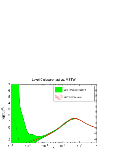
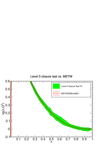
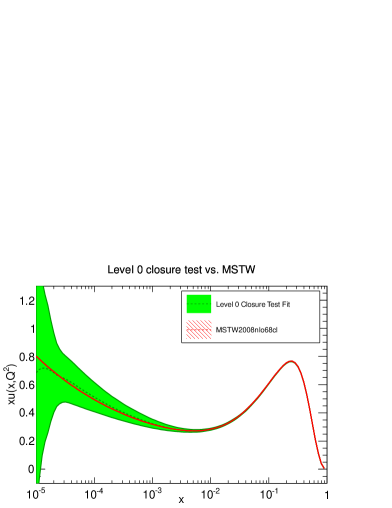
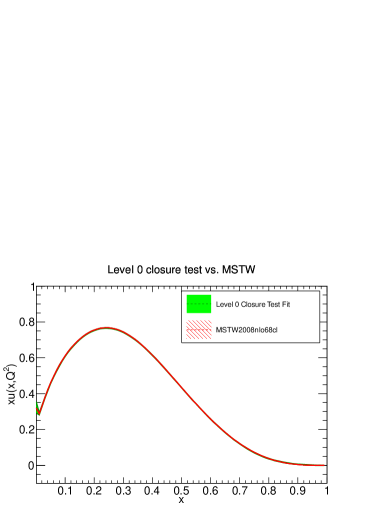
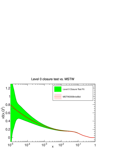
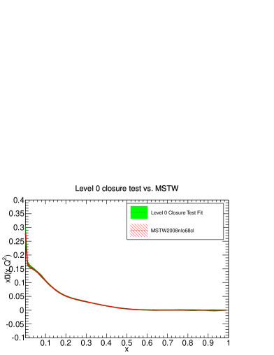

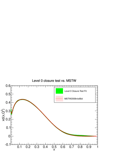
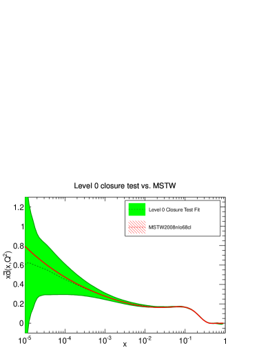
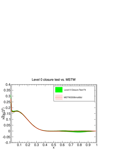
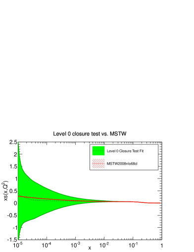
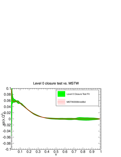

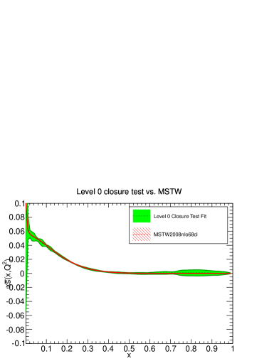
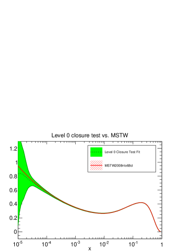

Additional interesting information can be extracted from Level 0 fits by looking at the PDF uncertainties of the resulting fit, computed as usual as the standard deviation over the sample of fitted replicas, either at the level of parton distributions or at the level of physical observables. Recall that at Level 0 the only difference between each of the replicas is the random seed used to initialize the minimization, and therefore, their spread quantifies different possibilities of approaching the underlying input PDFs. Given that the Level 0 input pseudo-data do not fluctuate, the cross-sections computed from the fitted PDFs must converge to these input values for each replica as the training length is increased; i.e. the uncertainty on the predicted value for all the observables included in the fit must go to zero.
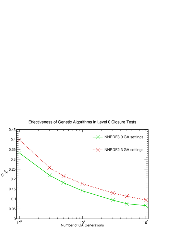
To verify this expectation, it is convenient to define an indicator which measures the standard deviation over the replica sample in units of the data uncertainty. This can be defined as follows:
| (24) |
To see that this does the job, consider the first term in Eq. (24) in more detail: using the definition of the in Eq. (19), we find that
so that
| (25) |
Thus in terms of the covariance matrix of the theoretical predictions
| (26) |
we have
| (27) |
i.e. the average over all the data points of the uncertainties and correlations of the theoretical predictions, , normalized according to the corresponding uncertainties and correlations of the data as expressed through the covariance matrix . If the covariance matrix was diagonal, i.e. in the absence of correlations, this would just be the variance of the predictions, divided by the experimental variance, averaged over data points; is thus recognized to provide the generalization of this in the presence of correlations.
In Fig. 8 we show , Eq. (24), for the Level 0 fits as a function of the length of the genetic algorithms minimization. As before, we compare the results for the GA settings used in NNPDF3.0, with the corresponding GA settings used in the NNPDF2.3 fit. We can see that indeed, as we increase the training length, the spread of the theoretical predictions at the data points for different replicas at the level of fitted cross-sections decreases monotonically, and again here we observe the improvement from the more efficient minimization strategy in NNPDF3.0. Specifically, for the longest training length we find that standard deviation of the theoretical predictions is on average almost by a factor 20 smaller than the nominal standard deviation of the data.
On the other hand, the fitted PDFs themselves need not become identical replica by replica, even at Level 0, since different functional forms for the PDFs can yield the same predictions for the observables. Of course, in the kinematic regions where data are available, the fluctuations of the PDFs are limited by the fact that the neural networks provide a smooth interpolation between points that are constrained by data. In this respect, in regions where the PDFs are well constrained by experimental data, PDF uncertainties should be very small, and indeed they are.
This is however not necessarily the case in the extrapolation regions, where we expect large PDF uncertainties, which moreover are essentially independent of the training length. This is due to the fact that there the functional forms can vary substantially without affecting the fitted figure of merit, . These two effects, very small PDF uncertainties in the data region, and large PDF uncertainties in the extrapolation regions, in particular at small and large are still clearly visible in the plots in Fig. 6, even at the end of a 100k-generation training. These results provide a way of quantifying the extrapolation uncertainty on the PDFs due to the lack of direct constraints in these regions: this is an irreducible source of PDF uncertainty that can only be reduced if new data is provided, and that accounts for most of the PDF uncertainties in the fits to real data in the extrapolation regions.
4.2.2 Effective preprocessing exponents
When using as an input to the closure test a PDF set based on a relatively simple functional form, such as for example MSTW08 [138] or CT10 [150, 151], the exponents that characterize the asymptotic small- and large- behavior of the individual PDFs are known, since they are part of the set of parameters defining the PDF parametrization at the initial scale. For instance, in the MSTW08 fit, the PDFs are parametrized at the initial scale of 1 GeV2 using a generic functional form and therefore, the asymptotic small- and large- behaviors will both be powerlike, parametrized by the exponents and . Note that in general one has to be careful with this naive interpretation since sub-asymptotic corrections can be numerically large.
In the context of NNPDF fits, no explicit assumption is made on the functional form of PDFs, which are instead parametrized using neural networks. On the other hand, preprocessing is introduced in order to absorb the dominant behavior of the fitted PDFs at small- and large- and speed up the fitting. As explained in Sect 3.2.2, when fitting real data, the range in which preprocessing is varied for each PDF is determined dynamically through an iterative procedure.
In the context of a Level 0 closure test, when a PDF set based on a known functional form is used as input, it is interesting to verify that the small- and large- behavior of the fitted PDFs reproduce the ones of the input PDFs. This can be achieved by comparing the effective preprocessing exponents between the fitted and input PDFs. These effective exponents can be computed as in Eq. (11-12). The results of this comparison are shown in Fig. 9, for the Level 0 closure test with 100K generations (fit C7 in Table 8). A beautiful agreement is found, with the MSTW08 value always within in the one-sigma band of the fitted PDFs, thus showing that our methodology is capable of precise quantitative predictions on the behavior of the functions that we are trying to fit. Similar results are obtained for all the other PDF combinations.
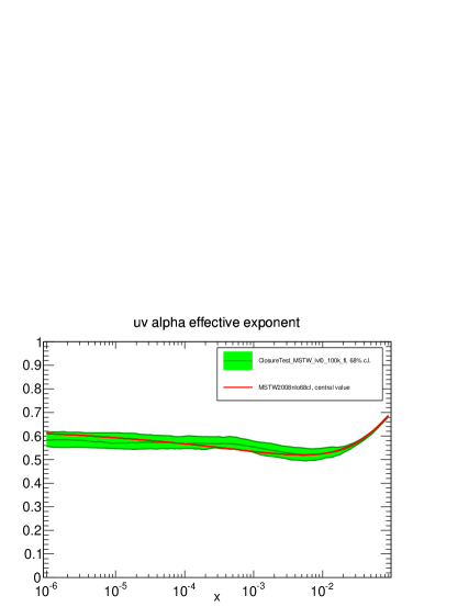
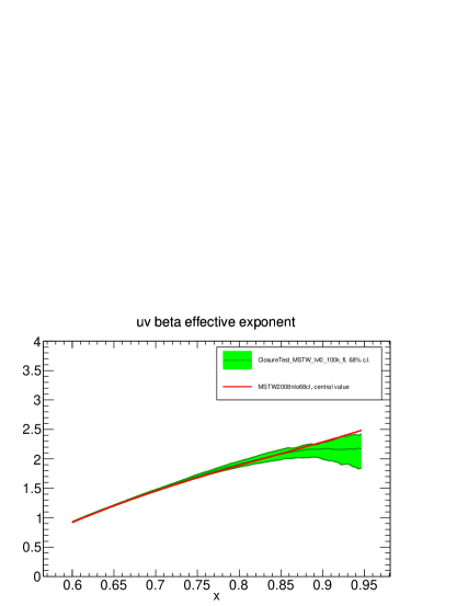
4.3 PDF uncertainties in closure tests
In the previous section we studied Level 0 closure tests, in which the fit quality can become arbitrarily good, and the PDF uncertainties arise purely due to the fact that the experimental data used in the fit has finite kinematical coverage. Now we turn to Level 1 and Level 2 closure tests, and in doing so we shed some light, in the cleanly controlled environment of closure testing, on the various different origins of PDF uncertainties: specifically those due to the fluctuations of the experimental data, to the choice of functional form, and to the extrapolation uncertainties due to the finite coverage of the data. Following this, we go on to quantify how well the closure test is passed, both in terms of central values and uncertainties, using various statistical estimators.
4.3.1 PDF uncertainties: data, functional and extrapolation components
A more sophisticated understanding of the various sources that form the total PDF uncertainties can be obtained in the context of closure tests by comparing Level 0, Level 1, and Level 2 fits. Indeed, in each of these fits the PDF uncertainty band has different components. In Level 0 fits, the only significant component is the interpolation and extrapolation uncertainty (which we will refer to as extrapolation uncertainty for short); in Level 1, one also has the uncertainty due to the choice of functional form; and in Level 2 finally one also adds the uncertainties due to the fluctuations of the experimental data. Therefore, by comparing Level 0, Level 1 and Level 2 closure fits we can analyse how the total PDF uncertainties are decomposed into data, functional and extrapolation uncertainties.
Let us begin with the extrapolation uncertainty. As discussed in the previous section, in a Level 0 closure test, the PDF uncertainty at the fitted data points should go to zero as the training length is increased. This implies that, in the experimental data region, PDF uncertainties should also decrease monotonically as a function of the training length wherever data are available. However, in between data (interpolation) and outside the data region (extrapolation) PDFs can fluctuate. This residual uncertainty, which remains even at infinite Level 0 training length, we refer to as the extrapolation uncertainty.
Note that, given the highly non-trivial dependence of PDFs on the measured cross-sections, and the wide range of observables included in the fit, it is very difficult to determine precisely how this extrapolation region is defined: while a non-negligible extrapolation component is expected for all PDFs at small enough and large enough values of , significant uncertainties due to interpolation could also be present at intermediate . In fact, this also accounts for possible degeneracies between PDFs: for example, even in Level 0 closure fits some PDFs can compensate each other to produce exactly the same cross-section, and this effect will also be included in the extrapolation uncertainty.
To illustrate this point, in Fig. 10 we show the results of Level 0 closure tests for all PDFs, for three fits with identical settings but different training length, 5k, 30k and 100k GA generations respectively. We can see that while the uncertainties at 100k generations are smaller than at 5k, they do not go to zero, and in fact for very small or very large values of , where there is no experimental information, they remain very large. This is a direct consequence of the lack of experimental data in this region, and illustrates this irreducible component of the PDF uncertainties that we denote as extrapolation uncertainty. Furthermore, in most of the data region (with the possible exception of a very small region around the valence peak for the up and down distributions) the uncertainty at 30k generations and 100k generations are very close, and in particular rather closer than the corresponding values of Fig. 8. This is especially noticeable for the up and gluon distributions, and it means that, even in the data region, there is an irreducible component of the uncertainty which does not go to zero even for extremely long training length, and can only be reduced with more data, as it is due to the interpolation between data points. Otherwise stated, at 30k, the uncertainty of the Level 0 fit shown in Fig. 8, which is evaluated only at the data points and is thus due to fitting inefficiency, is already subdominant in comparison to the extrapolation uncertainty almost everywhere.
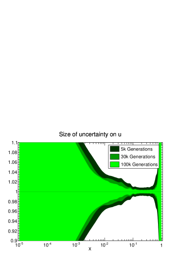
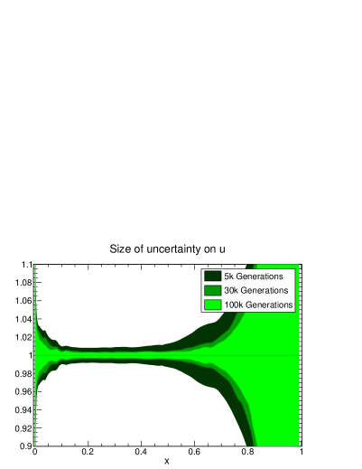
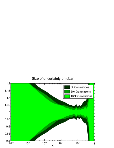
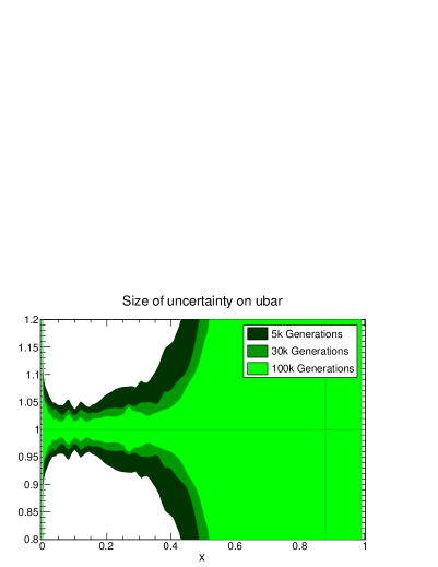
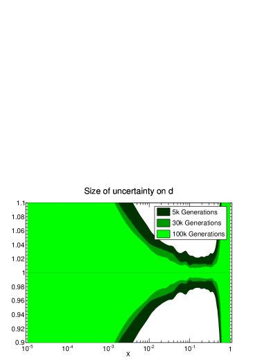
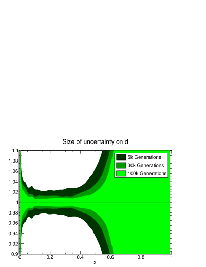
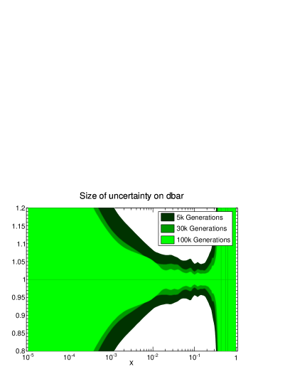
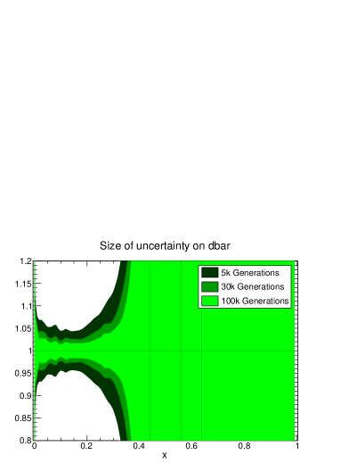
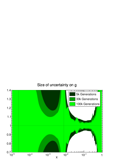
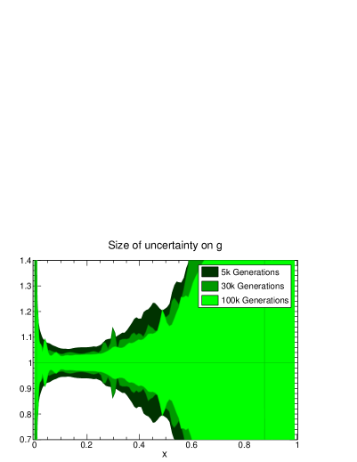

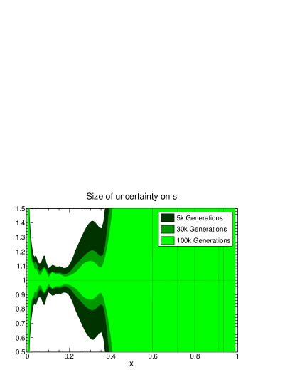
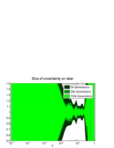

Now we can see how the total PDF uncertainty also contains functional and data uncertainties by comparing the results of Level 0, Level 1 and Level 2 closure tests with otherwise all other fit settings identical. Figure 11 shows the ratios of the uncertainty of the fitted PDFs to the respective central values in each case, for the C5, C8 and C9 closure test fits, see Table 8, corresponding to Level 0, Level 1 and Level 2 closure tests respectively. The MSTW08 NLO set is used as input PDF , and a total training length of 30k generations is used in all cases. For the three fits, the PDF uncertainty bands are defined as the 68% confidence interval from the sample of fitted replicas. Results are provided for the PDFs in the flavor basis at the input parametrization scale of , though the qualitative interpretation is the same in any other basis.
In order to understand these results, it is useful to review our expectations for the results of the Level 1 and Level 2 closure fits, as we have done above for Level 0. In a Level 1 fit, the central values of the data have been fluctuated around the theoretical prediction, and therefore no longer provides an absolute minimum for the . Indeed, provided the PDF parametrization is flexible enough, the minimization algorithm should find a large number of different functional forms that yield an equally good . Therefore, in Level 1 closure fits, on top of the extrapolation component, the total PDF uncertainty will include a new component, which we refer to as functional uncertainty.
This functional uncertainty is a consequence of the fact that, as discussed in Sect. 3.3.2, the optimal in the presence of data fluctuations is not the absolute minimum of the . In a closure test, this is obvious: the optimal result corresponds to the true underlying functional form, and thus the optimal is the one of the Level 1 pseudo-data, whose value is of order one (and tends to one in the limit of infinite size of the data sample). For an infinite-dimensional space of functions, this value can be obtained in an infinity of different ways, whose spread provides the functional uncertainty. The look-back method discussed in Sect. 3.3.2 ensures that regardless of the length of the fit, the final does not decrease beyond the overlearning point, and thus again this functional uncertainty will survive even for infinite training length.
In a Level 2 fit, the starting point is again the Level 1 pseudo-data generated by adding a Gaussian fluctuation over the predictions obtained from the input PDFs. Now however there is a second step, which reproduces the actual fitting strategy used in the NNPDF framework: starting from these pseudo-data, a set of Monte Carlo replicas is generated that reflects the statistical and systematic errors given by the experimental measurements. Because each replica fluctuates around Level 1 data, the expectation for the minimized figure of merit for each replica in Level 2 fits is , although we still expect . In Level 2 closure tests, each replica is fitted with exactly the same algorithm, yielding an ensemble of fitted PDFs whose statistical properties are a faithful propagation of the fluctuations in the underlying dataset. The increase in the uncertainty from Level 1 to Level 2 fits is the genuine data uncertainty.
Following these considerations, it is possible to understand quantitatively the features that are observed in Fig. 11. Firstly, we see that Level 0 uncertainties are smaller than Level 1 and in turn these are smaller than those at Level 2: this confirms the expectation that at each Level we are adding a new component of the total PDF uncertainty, extrapolation, functional and data components, respectively. We also observe that in the small- and large- regions it is the extrapolation uncertainty that dominates, that is, the Level 2 PDF uncertainties are already reasonably reproduced by those of Level 0 closure fits.
However, as already noticed from Fig. 10, the Level 0 extrapolation component can be significant also in some regions with experimental data, like medium , due to interpolation and degeneracies. Indeed, it is clear from Fig. 11 that the Level 0 uncertainty in the data region is typically of order of 5% or more, and only goes down to about 1% in a very small region close to the valence peak for the up and down quark distributions. But we know from Fig. 8 that on average the uncertainty at the data points is by about a factor (for a 30k fit) smaller than the uncertainty of the original experimental data , i.e. it is of order of 1-2%. This uncertainty is due to fitting inefficiency, but anything on top of that, i.e. the Level 0 uncertainty seen in Fig. 11 except for the up and down quarks at the valence peak, is a genuine extrapolation uncertainty.
By comparing to the Level 1 results, we see that the functional uncertainty is generally sizable, especially in regions at the boundary between data and extrapolation, in particular at large . Interestingly, in regions where we have a rather reasonable coverage from available data, the three components are roughly of similar size. Take for example the gluon around , which is well constrained by the high-precision HERA measurements. We see that the extrapolation, functional and data uncertainties are all of similar size, and thus a proper estimate of the total PDF uncertainty must include all three components. The same applies for other PDF flavors, such as for example strangeness for (with abundant constraints from neutrino DIS and LHC data) or the up and down quarks at medium and large- (with many DIS and LHC datasets providing information on them).
An important general conclusion is that data uncertainties are not dominant anywhere, and thus a PDF determination that does not include the extrapolation and functional components will underestimate the overall PDF uncertainty. This conclusions is consistent with that of previous rather less sophisticated, NNPDF studies such as those of Ref. [152]. It is natural to conjecture that the tolerance method [153] which is used in Hessian fits, provides an alternative way of supplementing the data uncertainty with these extra necessary components.
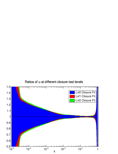
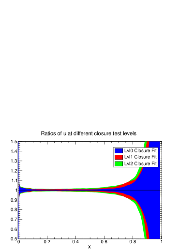


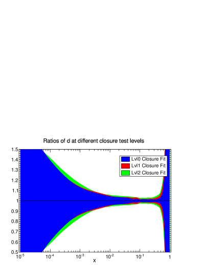
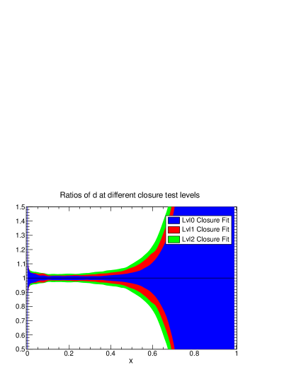
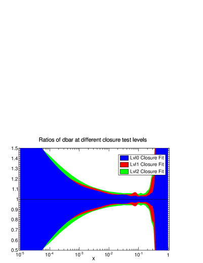
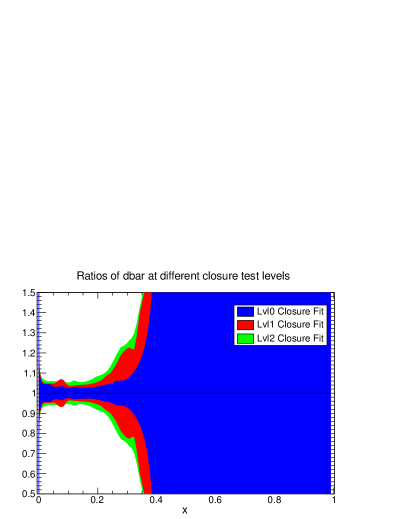
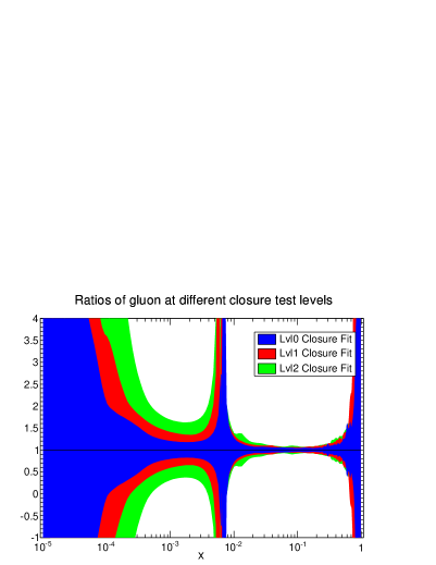


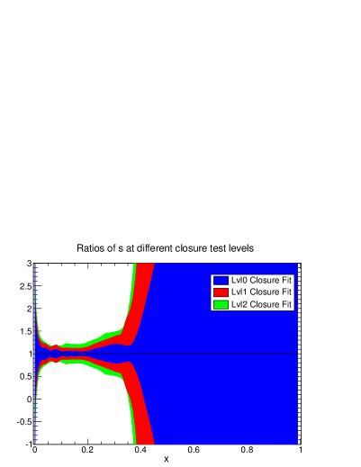
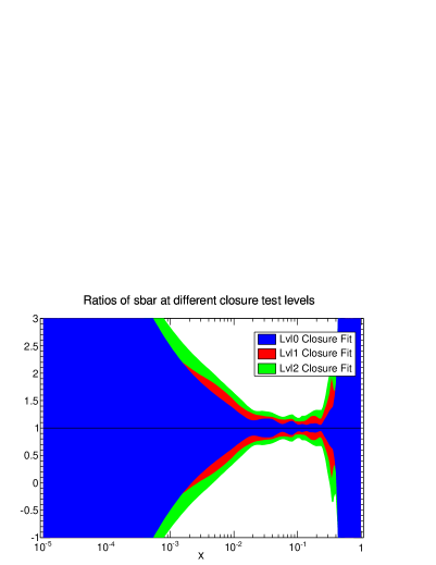
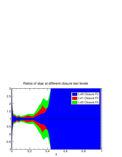
4.3.2 Quantitative validation of PDF uncertainties in closure tests
In the previous section we discussed the various components of the total PDF uncertainty in a purely qualitative way, by comparing the results of Level 0, Level 1 and Level 2 closure tests. In this section we provide some quantitative estimators of the successfulness and effectiveness of the closure tests, which will be used in Sect. 4.4 to validate the closure test fits.
In Level 1 and Level 2 closure fits, we expect that the central obtained from the average of the fitted PDFs should reproduce the one computed using the input PDFs, that is where by we indicate that that we use the Level 1 pseudo-data, which include the fluctuations.
We can test for a particular fit whether this is the case by defining the following statistical estimator
| (28) |
that is, the difference between the central of the closure test fit, computed with an average over replica PDFs, and the of the input PDF set, both computed with respect to the same closure test dataset. This estimator is therefore a measure of how close the closure test fit reproduces the theoretical predictions of the input PDF, and therefore it provides a quantitative measure of the success of the test.
In particular, noting that in genetic algorithm minimization is a decreasing function along the training, corresponds to underlearning (the optimal has not been reached yet), corresponds to perfect learning of the underlying law, while in fixed-length genetic minimization would correspond to overlearning, i.e., the fit is learning the noise in the data. Of course in a closure test the true underlying is known and thus one could stop at the optimal point by comparing to it, which of course is not possible in a realistic situation. The effectiveness of the method for determining the optimal stopping point that is actually used — in our case, the look-back method described in Sect. 3.3.1 — can then be measured by simply evaluating how close Eq. (28) is to zero at the actual stopping point. The estimator Eq. (28) thus quantifies how successful the closure test fit is in terms of reproducing the central values of the input PDFs.
We now introduce an estimator which allows for an assessment of the accuracy with which PDF uncertainties are reproduced. To this purpose, we first recall that for an unbiased estimator, assuming gaussianity, the -sigma intervals about the prediction can be interpreted as confidence levels for the true value (see e.g. Ref. [15]): this means that the true value must fall on average within the one sigma uncertainty band in 68.3% of cases, within the two-sigma band in 95.5% of cases, and so on.
We thus define the estimator
| (29) |
where is a positive integer, and , and are the number of PDF flavors, values and fits respectively, over which averages are performed. For the sampling of the PDFs in , we use 20 points between and 1, half of them log spaced below 0.1 and the rest linearly spaced. In Eq. (29), denotes the indicator function of the interval : it is only non-zero, and actually equal to one, if its argument lies in the interval , while it vanishes for all other values of its argument. Finally, and are the average PDFs and the corresponding standard deviation of the PDF flavor for fit , computed over the sample of replicas of fit . The estimators provide the fraction of those fits for which the input PDF falls within one sigma, two sigma, etc of the central PDF , averaged over PDF flavors and values of . In a successful closure test we should thus find that , , etc.
In principle, in order to calculate , Eq. (29), we would need to, for instance, generate 100 closure test fits each one with replicas, following the procedure explained above. However performing this very large number of fits is very computationally expensive, and we would instead like to obtain an estimate of which involves fewer fits. To achieve this, we can approximate the mean of each fit, , by fitting a single replica to each set of closure test data at Level 1, i.e. without additional replica fluctuations. We can also replace the individual values of in Eq. (29) with the corresponding values taken from a single 100 replica fit, making use of the fact that the variation in the PDF uncertainties between different closure test fits is small.
4.4 Validation of the closure test fits
Using the statistical estimators introduced in the previous section, we now move to validate quantitatively the results of the closure fits. First, we show how close the central values and values of the input and fitted PDFs are to each other, both for the total dataset and for individual experiments. Then we discuss a quantitative validation of the PDF uncertainties obtained in the closure tests, using the estimators defined in Sect. 4.3.2 for this purpose. Finally in this section we will show how one can also use the Bayesian reweighting procedure [18, 154] to provide further evidence that the closure tests are working as expected. Indeed, it turns out that reweighting provides the most stringent validation test, since for it to be successful it is necessary to reproduce not only central values and uncertainties, but also higher moments and correlations.
4.4.1 Central values
A first indicator of the quality of a closure test is provided by the values of the central obtained using the fit, . This should reproduce the values of the obtained using the generating PDFs, that is . For our baseline Level 2 closure test, using pseudo-data based on MSTW08, and performed with the look-back stopping criterion rather than at fixed length (fit C9 in Table 8), we obtain the following result for Eq. (28),
| (30) |
which shows that the fitted PDFs reproduce the of the generating PDFs at the 1% level, with a small amount of overlearning, which must be viewed as an inefficiency of the look-back method. The result for the corresponding Level 1 fit (C8) is very similar: .
This level of agreement is achieved not only for the total , but also for the individual experiments included in the global fit. This is important to test, since each experiment fluctuates by a different amount, and we want the closure test to reproduce these fluctuations. Figure 12 shows the contributions in the Level 2 fit C9 to from the pseudo-data generated for each individual experiment, compared to the corresponding contributions to . The horizontal bars show the total for the two PDF sets, and are computed as the weighted average of the of each individual dataset. The datasets shown are the same used in the baseline NNPDF3.0 global fit (see Tables 1 and 2 in Sect. 2).
We see from Fig. 12 that the closure test successfully reproduces the of the input PDFs, MSTW08, not only for the total dataset but also experiment by experiment. Note that especially for experiments with only a small number of points the fluctuations added to the pseudo-data can lead to a quite different from one, and this is exactly reproduced by the closure test results. Figure 12 is thus a strong check that, at least at the level of central values, the Level 2 closure fits are successful.
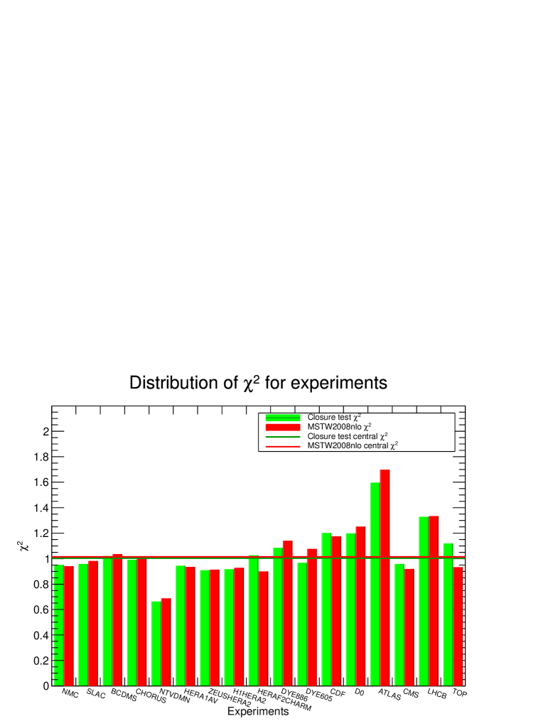
4.4.2 PDF uncertainties: qualitative validation
We can get a first assessment of the uncertainty of the Level 2 closure fit by means of the estimator Eq. (24). For the Level 2 closure fit C9 we get
| (31) |
a result that indicates that the PDF uncertainty on the data points from the Level 2 closure fits is roughly a factor of four smaller than that the original experimental uncertainty, due to the combination of all the data into the PDFs. For the Level 1 fit C8 this number is rather smaller: , confirming that at Level 1 the data uncertainty is still missing. Since contributions to are entirely from the data points, there is no extrapolation uncertainty; however, the Level 0 uncertainty, though small, is not exactly zero because this would require infinite training length. From Fig. 8 we may read off that the Level 0 contribution to is of order of . Hence, combining uncertainties in quadrature, we get that the contribution of the functional uncertainty to is about , and the data uncertainty contribution is about , so, at least on average, the data and functional uncertainties are of comparable size.
Recalling that is essentially the ratio of the uncertainty of the fitted PDFs at the data points to that of the original data, we conclude that the fitting procedure leads to an error reduction by a factor of four or so. However, we must now verify that this error reduction is real, namely that uncertainties are correctly estimated by the closure test. We do this first in a more qualitative way, and then more quantitatively in Sects. 4.4.3 and 4.4.4 below.
To this purpose, we first look at the distance between the fitted PDFs and the underlying “truth” in units of the standard deviation. This is most efficiently done using the distance estimators, as defined in Appendix B, between the closure test fit PDFs and the input MSTW08 PDFs. The distances between fitted and input PDFs in closure tests are normalized such that corresponds to agreement at the one-sigma level (in units of the uncertainties of the closure test fitted PDF), corresponds to agreement at the two-sigma level and so on, that is,
| (32) |
where stands for the PDF flavor. In the following, distances are computed at the initial parametrization scale of .
Using the definition Eq. (32), the distances between the central values of the fitted and the input PDFs (MSTW08) in the Level 2 closure test C9 are shown in Fig. 13. The distances in Fig. 13 show that the fitted and input PDFs are in good agreement, at the level of one sigma or better (in units of the uncertainty of the fitted PDF), with some PDFs for some points in differing by an amount between one and two sigma, as one would expect if the underlying distribution was roughly Gaussian. In the extrapolation regions, at small and large , the distances between input and fitted PDFs become smaller because of the large PDF uncertainties in these regions.

From the distance comparisons of Fig. 13 we can see that, at the qualitative level, the closure test is successful since the fitted PDFs fluctuate around the truth by an amount which is roughly compatible with statistical expectations. More insight on this comparison is provided by plotting, for all PDF flavors, the ratio between the fitted and input PDFs, including both the fitted PDF central values and uncertainties. This comparison is shown in Fig. 14 for each parton flavor. It is clear from these plots that the NNPDF methodology reproduces successfully the input PDFs, with deviations from the input functions usually by two standard deviations at most. This comparison provides further evidence that PDF uncertainties are properly estimated in Level 2 closure tests, in that the central value of the fitted PDFs fluctuates around the truth by an amount which is consistent with the size of the PDF errors.
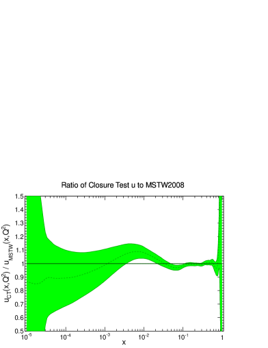
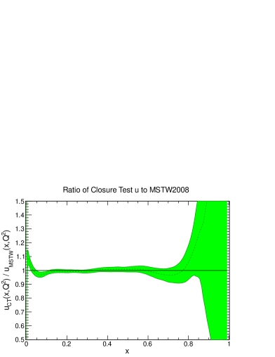
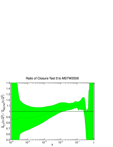
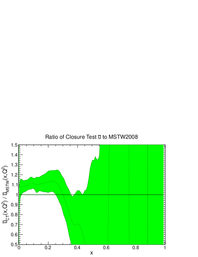

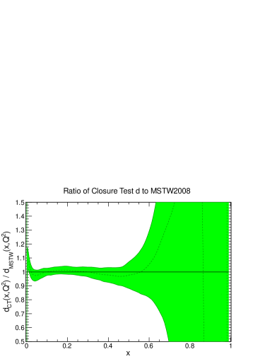
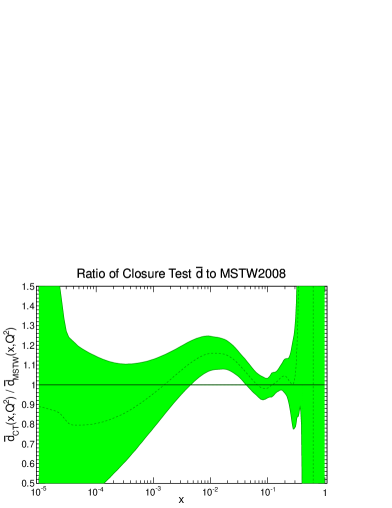
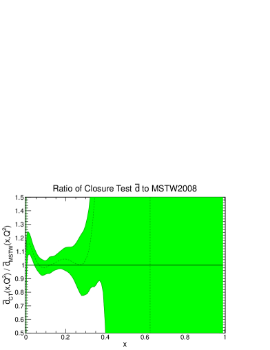

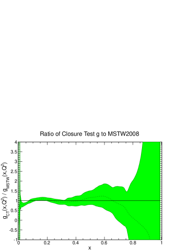
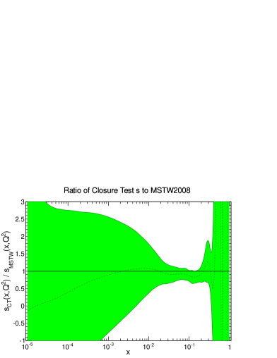
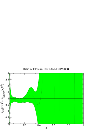
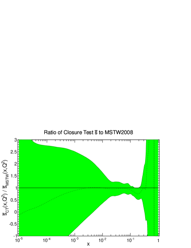
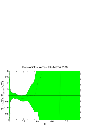
A final qualitative comparison can be performed by using the arc-length, which, as discussed in Sect. 3.3.2, provides a measure of the complexity of a function defined over a finite interval. A function that has a more complicated structure is expected to have a larger arc-length, and vice-versa. In the context of our fits, PDFs with too large arc-lengths might be an indication of over-fitting, with a PDF trying to use a contrived shape in order to fit statistical fluctuations. For this reason, as explained in Sect. 3.3.2, replicas that at the end of the fit have some PDFs with unnaturally large arc-length are discarded from the final sample.
In the context of closure tests, comparing the arc-lengths of the fitted PDFs with those of the input PDFs provide an integrated comparison, rather than point by point, that the fitted PDFs reproduce the input ones. The arc-lengths of the Level 2 fit C9, using MSTW08 as input, are shown in Fig. 15. Arc-lengths are computed at the input parametrization scale of GeV2. As expected from the comparison at the level of PDFs, there is also good agreement between the input and fitted PDFs at the level of arc-lengths, the arc-length of the input PDF typically lying within the 68% confidence level of the fitted PDFs.
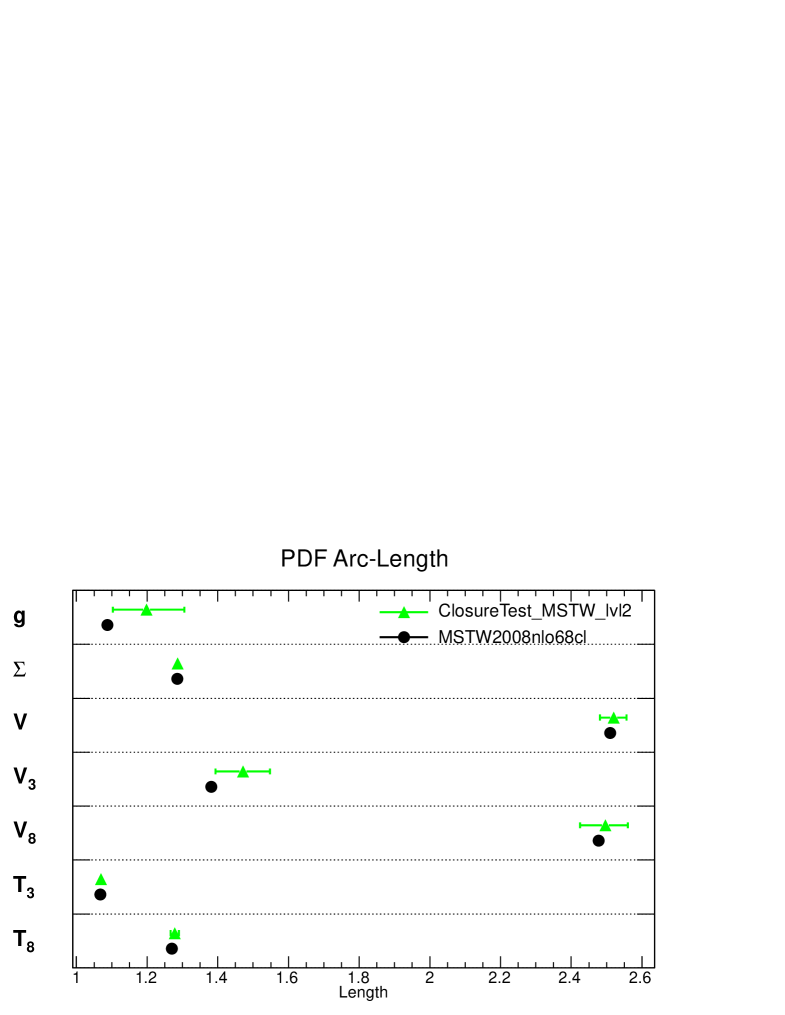
4.4.3 PDF uncertainties: quantitative validation
The results of Sects. 4.4.1 and 4.4.2 provide evidence the Level 2 closure tests are successful, both in terms of central values and of PDF uncertainties. We now provide a more quantitative assessment of this success using the indicators described in Sect. 4.3.2.
In order to validate quantitatively the agreement in central values we compute the estimators Eq. (29) for Level 2 fit C9. We obtain the following results:
| (33) |
to be compared with the theoretical expectations of 0.68 and 0.95. This excellent agreement confirms that the PDF replicas obtained by our fitting methodology can indeed be interpreted as a representation of the probability distribution for the PDFs given the data used in the fit.
To verify that this agreement is not accidental, or a fluke of the definition of the estimator , but rather a robust feature of our analysis, we have redone the whole procedure but this time based on Level 1 closure fits, set up in the same way as C8, and computed again the estimators. We already know from the qualitative comparisons between Level 1 and Level 2 uncertainties from Fig. 11 that in Level 1 closure tests PDF uncertainties are underestimated, and therefore in this case the central value of the fitted PDF will fluctuate more than its estimated uncertainty would suggest.
This implies that in Level 1 closure tests we expect the estimators to be smaller than the theoretical expectations above. Indeed, computing and at Level 1 this is precisely what we find:
| (34) |
which shows that indeed the Level 1 closure tests fail, in the sense that Level 1 fits underestimate PDF uncertainties. This confirms that the Level 2 step, that is the generation of Monte Carlo replicas on top of the pseudo-data with the fluctuations, is essential to obtain the correct PDF uncertainties.
The fact that the Level 2 closure test leads to a correct estimate of the PDF uncertainties, while the Level 1 fails, can be tested in more detail by looking at the distribution of the mean of our fit for different closure test datasets: this tests not only the one- and two-sigma confidence intervals, but the shape of the whole distribution of deviations between the prediction and the truth. Figure 16 shows the histograms of the differences between obtained using different closure test datasets (that is, pseudo-data generated with different random seeds) and the central value of the MSTW input PDFs, in units of the standard deviation of a standard Level 1 or Level 2 closure test. The histogram is generated using the values at , 0.1 and 0.2 for each PDF, as a representative sampling. The resulting distribution is very close to a Gaussian distribution with standard deviation 1 when scaled with the Level 2 uncertainties, and is considerably wider using the Level 1 uncertainties. This is consistent with the results found above that Level 2 uncertainties reproduce the correct fluctuations of the central values while Level 1 underestimates them.
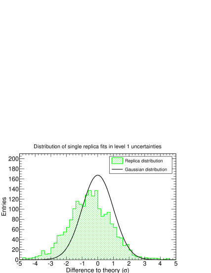
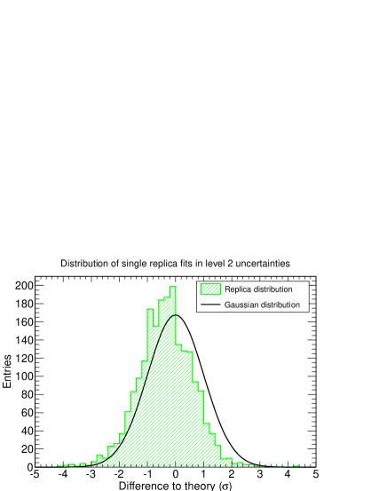
4.4.4 Closure test validation using Bayesian reweighting
The results above show that our Level 2 closure tests are successful in terms of both central values and uncertainties, both at the qualitative and quantitative levels. However, it is still conceivable that they could fail for higher moments of the fitted distribution, including the correlations. In this respect, the most stringent validation of our fitting methodology, also in the context of closure tests, is provided by exploiting the Bayesian reweighting method [154]. Reweighting allows one to determine a new set of PDFs from a prior set when new data are added. Since reweighting is analytic, in the sense that the weights are computed using the to the new data without the need for refitting, by comparing the reweighted distribution to a refitted distribution in a closure test, one can test rather precisely the fitting methodology.
With this motivation, we have performed, based on closure tests, two reweighting analyses, one at Level 1 and the other at Level 2. The priors consist in each case of sets of PDF replicas, produced using the same dataset as was used in the NNPDF2.3-like fits described in Sect. 5, in particular without the inclusive jet production data (which in NNPDF2.3 are from CDF and ATLAS). The pseudo-data were generated using MSTW08 as the input PDF, NLO QCD, and so on, just as for the C8 and C9 closure tests. They were then fitted in the usual way. The jet data were then included by reweighting the prior in the usual way [154], and the results compared with the corresponding closure test PDFs in which instead the jet data were included by generating pseudo-data, adding them to the prior pseudo-data and then refitting.
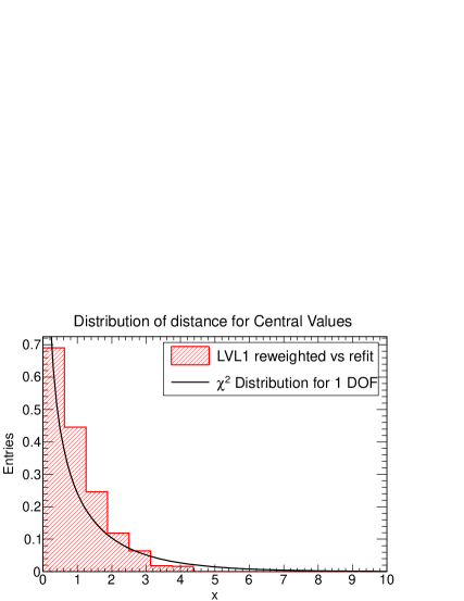

First, we compute the distance between the central values of the reweighted and refitted PDFs. The distribution of these distances, in both the Level 1 and Level 2 cases, is shown in Fig. 17. These distributions are obtained from a sampling produced using 100 points in for each PDF in the flavor basis, in the range between and 1. We expect this distribution of distances, for a successful reweighting test, to follow a distribution with one degree of freedom.
From Fig. 17 we see that the distribution of distances follows the statistical expectation of a distribution with one degree of freedom, as seen by comparing with the superimposed curve representing the latter, both in Level 1 and Level 2. This means that both Level 1 and Level 2 closure tests faithfully reproduce central values.
A more stringent test is obtained when computing uncertainties. The comparison between the reweighted and refitted results including uncertainties for Level 1 and Level 2 closure tests, are shown in Fig. 18. Several interesting conclusions can be drawn from this comparison. First, it is clear that at Level 2 the reweighted and refitted results are in perfect agreement, thus validating the procedure. Second, at Level 1 the refitted uncertainties are rather smaller than the reweighted ones, thus signaling a failure of the procedure.
The more interesting observation however is that in fact the Level 1 reweighted and Level 2 reweighted results essentially coincide. This, upon reflection, is to be expected: indeed, if the new data bring in sufficient new information, Bayesian reweighting produces results which are largely independent of the prior. Because the jet data are controlling the large- gluon uncertainty, and these are introduced by reweighting in both cases, this uncertainty comes out to be the same even when the uncertainties in the prior are not accurately estimated, as in the Level 1 fit. If instead the jet data are introduced by Level 1 refitting, the ensuing uncertainty comes out to be too small, because Level 1 does not properly account for the data uncertainty as discussed in Sect. 4.3.1.
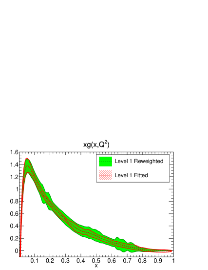
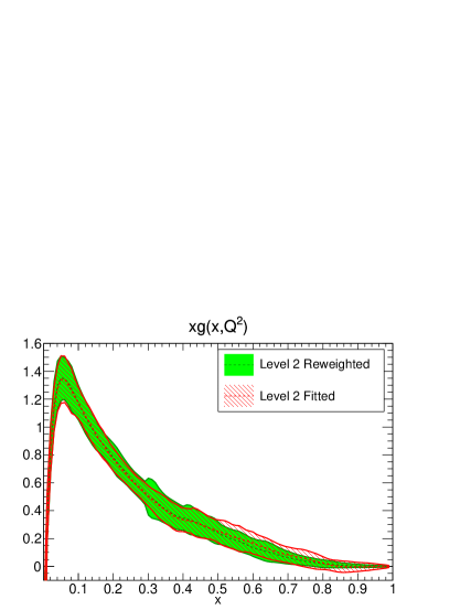
4.5 Robustness of the fitting methodology
We now turn to study the robustness of the fitting methodology against changes in some of its parameters, in the context of the closure test fits. The main advantage of using closure tests, as compared to attempting to address these issues in fits to real experimental data, is that any deviation from expectation must be attributed uniquely to deficiencies in the methodology, rather than blamed on spurious reasons like inconsistencies in the data, or failings of the theoretical description: in a closure test data and theory are by construction ‘perfect’.
First, we study how the fit results change when the training length is modified, then when the fraction of data included in the training set is varied, then we examine the effects of modifying the basis in which the PDFs are parametrized, and finally we verify that our baseline neural network architecture is redundant enough by comparing with the results of a fit with a huge neural network. Most of the closure tests in this section are performed using MSTW08 as input PDF, but we finally also explore the robustness of the closure testing against variations of this choice, in particular using CT10 and NNPDF3.0 itself as input PDFs.
4.5.1 Independence of the maximum number of GA generations
In NNPDF3.0, the cross-validation strategy that determines the optimal stopping point for the neural network training is based on the look-back method, described in Sect. 3.3.2. Provided that the maximum number of genetic algorithm generations is large enough, we expect results based on the look-back method to be independent of the value of . The condition for this to take place is that must be sufficiently large so that the look-back algorithm is able to the identify an optimal stopping point by finding somewhere close to the absolute minimum of the validation .
To verify this expectation, in Fig. 19 we show the distances for two Level 2 closure test fits with the maximum numbers of generations set to 30k and 80k (fits C9 and C11 in Table 8), all other settings being identical. Both fits use the look-back procedure to determine the ideal stopping point, and only differ in the maximum number of generations that are analysed by the look-back algorithm. Since the random seed used for the fit is the same in the two cases, this is completely equivalent to looking at the same fit had it been left to run for a larger number of generations.
Both the distances between central values, and the distances between uncertainties, are smaller than one for all the PDFs in the flavor basis over the whole range of values, showing that the two fits are statistically indistinguishable. We can therefore rule out any sizable dependence on the total training length in our current results, and we can stick to a baseline maximum number of generations of 30k in our fits to real data.
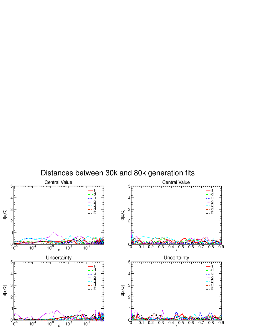
4.5.2 Dependence on the training fraction
As discussed in Sect. 3.3.2, the look-back cross-validation algorithm requires us to separate the fitted dataset into two disjoint subsets, the training set and the validation set, and in the standard fits each contains 50% of the total dataset. During the minimization, only the training set is seen by the neural network, with the validation being used only to determine the optimal stopping point. While the exact value of the training fraction would be irrelevant in the limit of infinite statistics, one could argue that for our large, but finite, dataset, results might change substantially if this 50% is varied to some other value. In particular, we must be sure that a training fraction of 50% is enough to retain all the relevant information contained in the original dataset.
In order to study the impact on the fitted PDFs of the use of a different training fraction, we have produced Level 2 closure fits with identical settings, the only difference being the value of this training fraction. Compared to the baseline fit with a training fraction of 50% (fit C9 in Table 8), we have produced a fit with a smaller training fraction, 25% (fit C13), and another one with a larger training fraction, 75% (fit C14). The comparison between these three values of the training fraction, quantified by the distance plots of Fig. 20 and Fig. 21, indicate that the resulting uncertainties on the fitted PDFs increase when the training fraction is reduced to 25%, showing that, for the NNPDF3.0 dataset, some of the information which is lost when using the smaller training fraction is not redundant. This effect can be quantified more directly by looking at the PDFs in the two fits, shown in Fig. 22. Is clear that the reduction of the training fractions entails a considerable increase of the PDF uncertainties.
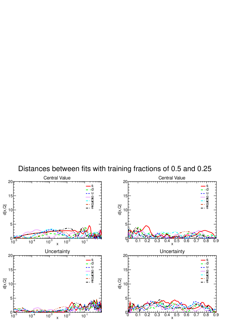
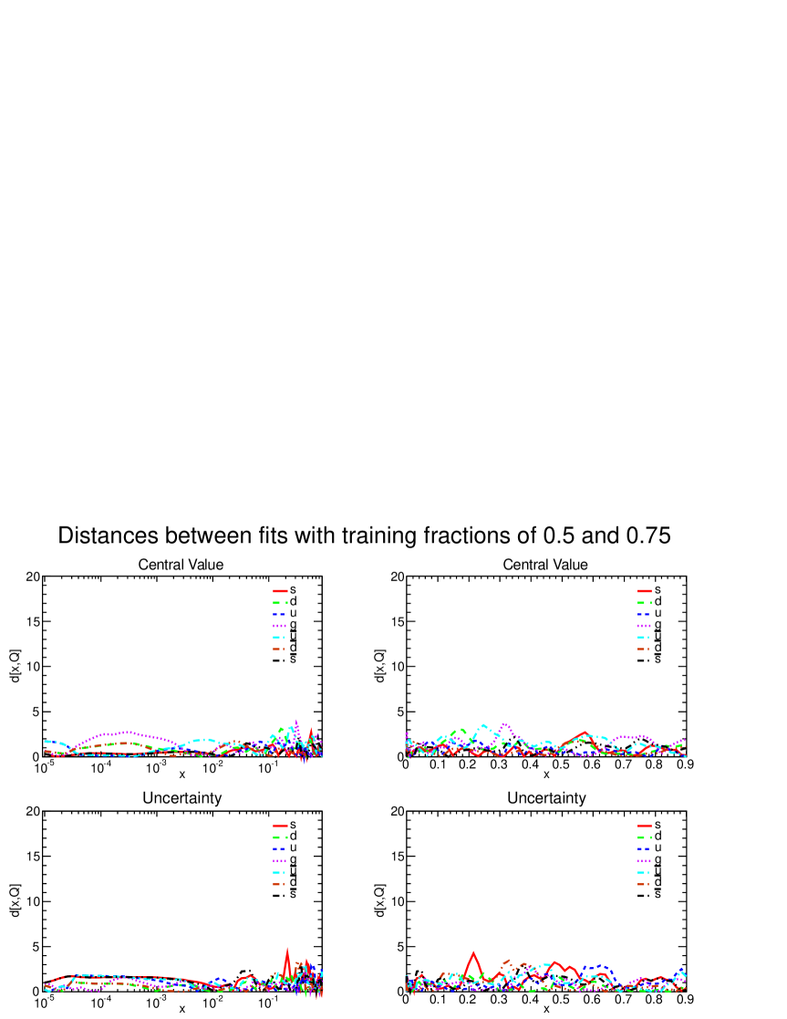
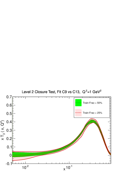
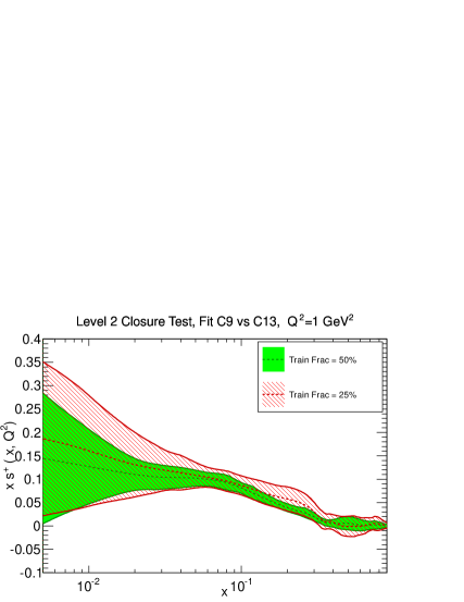
On the other hand, as can be seen from the distances in Fig. 21, the fits with training fractions of 50% and 75% are statistically indistinguishable. We thus conclude that the loss of information due to the training-validation splitting of the dataset required by the cross-validation procedure is small provided the training fraction is above 50%, but would be problematic for smaller training fractions.
4.5.3 Parametrization basis independence
One of the most attractive features of the new NNPDF3.0 methodology is that thanks to the new flexible C++ fitting code, it is possible to change the basis for the PDF parametrization rather easily, as discussed in Sect. 3.2. In turn, this allows us to perform detailed tests of the robustness of the whole fitting procedure: indeed, for a truly unbiased fit, results should be independent of the parametrization basis, since they are all related to each other by linear transformation. Note that in the standard Hessian approach to PDF fitting even adding a few extra parameters to the input parametrization can be quite complicated, let alone changing the parametrization basis altogether.
In order to test for this, we have produced a closure test Level 2 fit, C12 in Table 8, which is otherwise identical to fit C9 but uses the NNPDF2.3 parametrization basis, Eq. (7), rather than the new NNPDF3.0 parametrization basis, Eq. (8). The distances between fits C9 and C12, that is, between fits in the NNPDF3.0 and NNPDF2.3 parametrization basis, are shown in Fig. 23. We see that distances are quite small, though slightly larger than for statistically indistinguishable fits.
Distances are typically between and , so some slight differences due to the choice of basis are found, which are however much smaller than the corresponding PDF uncertainties: this means that basis independence is satisfied up to inefficiencies of the algorithm at the quarter-sigma level. Of course, this does not fully test for basis independence, as three of the basis combinations (singlet, triplet, and valence) are the same in the two bases which are being compared. However, it is worth noticing that PDFs with a relatively simple shape (with a single maximum) such as the strange combinations in one basis, are obtained as linear combinations of PDFs with a more complex dip-bump shape in the other basis: the stability of results then provides a strong check that the final PDF shape is independent of a bias due to the form of the parametrizing function. We can conclude that our results are independent for all practical purposes of the choice of fitting basis. As will be shown in Sect. 5.3.5, similar conclusions will be derived of the corresponding tests in the fits to real experimental data.
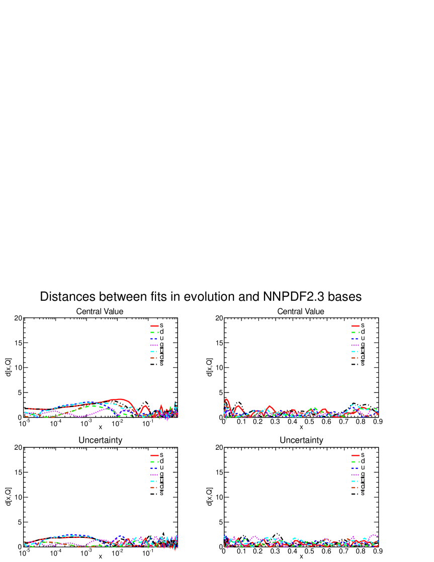
4.5.4 Redundancy of the neural network architecture
To be used as reliable unbiased interpolants, neural networks have to be characterized by an architecture redundant enough for the problem at hand: adding or removing nodes, even a substantial number of them, should leave the final results unchanged. The choice of a 2-5-3-1 architecture as baseline for the NNPDF fits can be justified precisely by showing its redundancy, as we did in previous work [6]. Using the closure testing technology, we have revisited for the current fits the stability of the fit results with respect to this choice of the architecture of the neural networks.
Starting from our baseline architecture, 2-5-3-1, which has 37 free parameters for each PDF, or 259 in total, we have performed a closure fit with instead a huge neural network, with architecture 2-20-15-1, therefore increasing by more than a factor 10 the number of free parameters in the fit. Other than this modification, exactly the same fit settings were used in the two cases.
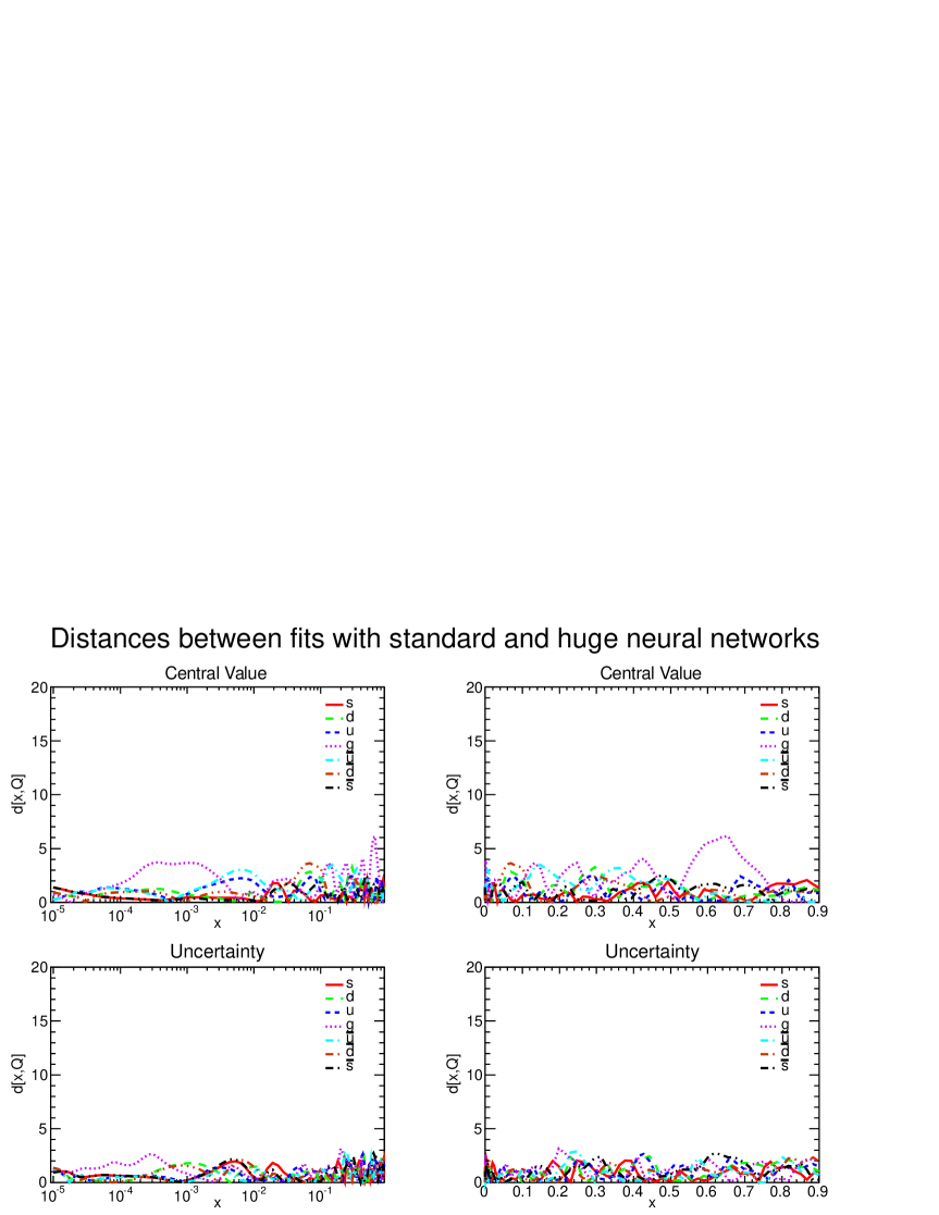
The distances between the two fits can be seen in Fig. 24. Remarkably, even increasing the architecture to have a factor 10 more free parameters, the fit using the huge networks is still quite close to the fit with standard sized networks. Again, we do not have perfect statistical equivalence, but inefficiencies are well below the half-sigma level.
This test also provides another demonstration of the resilience to over-fitting of our fitting methodology. Indeed, one might fear that such a large increase in architecture would lead to massive overlearning, while in actual fact results are virtually unchanged. This is thus a significant test of the effectiveness of the look-back method in determining the optimal stopping point.
Interestingly, we also observe a very moderate increase in CPU time when using the huge network as compared to our baseline architecture. This is because when a network is very redundant, it often makes little difference which parameters the algorithm changes.
Finally, let us mention that several other tests of neural network architecture were also performed, including changing the number of layers in the networks and the number of inputs. In most cases the results were either very similar to those from the standard structure or (for some smaller networks) noticeably worse.
4.5.5 Robustness with respect to the choice of input PDF set
So far in this section we have shown results fitted to the pseudo-data generated using MSTW08 as input PDF, and studied the effects of changing some of the settings of the closure test fits. However, it is important to verify that there is nothing special in using pseudo-data generated with MSTW08, and that our methodology is flexible enough so that similar successful closure fits are achieved if other PDFs are used as input. In particular, we want to explicitly verify that self-closure is successful: using NNPDF3.0 as input PDF, and checking that it is correctly reproduced by the closure fit. Note that the MSTW08 and CT10 parametrizations are relatively simple, so we need to verify that everything works fine even when a very flexible PDF parametrization is used as input in the closure test.
As a preliminary test, we have verified that Level 0 tests works regardless of the input PDFs, by producing a number of fixed length Level 0 fits for different input PDFs, and checking that all the conclusions of Sect. 4.2 are unchanged if input PDFs other than MSTW08 are used to generate the pseudo-data. We have then moved to Level 2 tests: we have performed closure test fits using exactly the same methodology as those based on MSTW08, but now using pseudo-data generated using different input PDF sets, in particular with the CT10 and NNPDF3.0 NLO sets. In the latter case, we have performed closure tests with and without the inclusion of the generalized positivity constraints described in Sect. 3.2.3. Given that NNPDF3.0 satisfies these constraints, this is a useful cross-check. These closure tests are labeled in Table 8 as C10 (for CT10) and C16 and C17 (for NNPDF3.0 without and with positivity constraints).
First, Fig. 25 shows the distances between the fitted and the input PDFs, Eq. (32), for the closure test fit which uses the CT10 NLO PDF set to generate the data. Let us recall, as discussed above, that these distances are normalized to the standard deviation of the fitted PDFs, and thus a value indicates that input and fitted PDFs agree at the one sigma level, and so on. These distances should be compared with the corresponding results obtained using MSTW08 as input, Fig. 13. We observe that, just as with MSTW08, the fitted PDFs are mostly within one sigma of the input PDFs, and never more than around two sigma away. In this respect, the closure test based on CT10 is as successful as that based on MSTW08. We have verified that this is also the case using some of the other estimators considered in this section.
The distances Eq. (32) are shown again in Fig. 26 now for a closure test fit using as input the NNPDF3.0 NLO PDFs. As in other closure tests, no generalized positivity is required here. This fit is therefore the ultimate closure test, providing evidence of self-closure, where the PDF set used to generate the pseudo-data has been determined using the same methodology as the closure test fit. Again, the agreement using NNPDF3.0 as input is as good as that obtained using other PDFs with a less flexible parametrization, showing that the closure tests works also in the case of a initial condition with substantial structure.
All of the closure test fits shown so far have been performed without the positivity constraints used in the fits to real data, described in Sect. 3.2.3. The motivation for this is that for some of the input PDFs used in the closure tests, in particular MSTW08, generalized positivity is not satisfied and therefore including such constraints would result in inconsistencies with the generated pseudo-data in the closure test, potentially biasing the results. On the other hand, as shown in Sect. 5.3.2, the NNPDF3.0 fits satisfy the generalized positivity constraints by construction, and therefore if we use NNPDF3.0 as input PDF we can include generalized positivity in the closure test, expecting to find no differences with respect to the previous case. Fig. 27 shows the distances, Eq. (32), for the closure test using as input the NNPDF3.0 NLO PDFs and now also with the generalized positivity constraints imposed during the closure test fit. We indeed find that the level of agreement is similar as that of the closure test when no positivity constraints were imposed during the minimization.

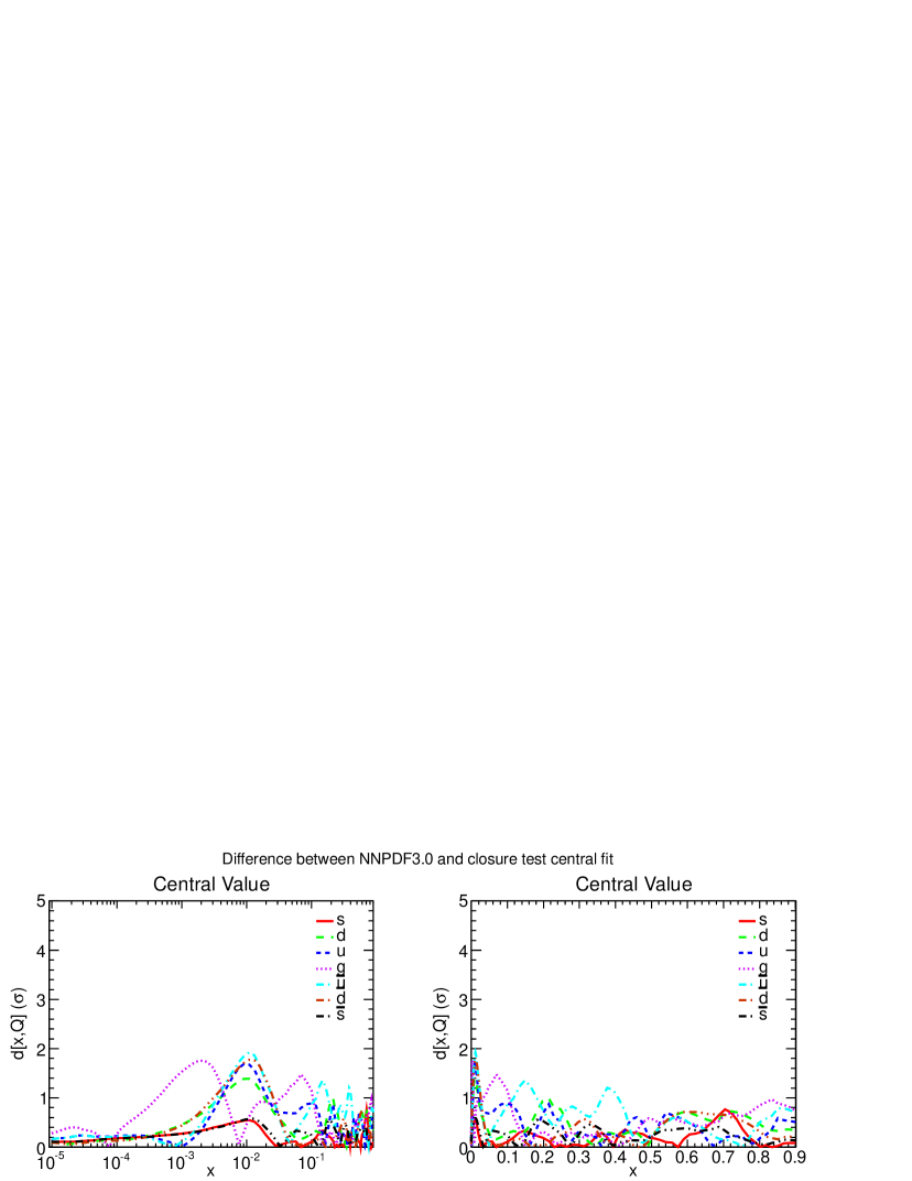
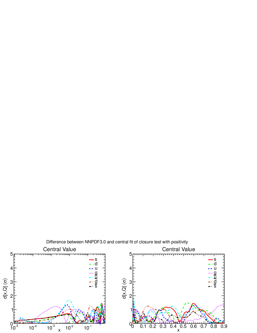
5 The NNPDF3.0 PDF set
In this section we present the NNPDF3.0 LO, NLO and NNLO global fits. First, we discuss fit quality and the dependence of the on its exact definition and on the treatment of systematic and normalization uncertainties. Then we show results for PDFs, we compare the new sets with NNPDF2.3 and with other existing PDF sets.
Next, we explore the dependence of the NNPDF3.0 partons on the choice of dataset. We propose a new definition of conservative PDF set, based on an estimator which allows for an assessment of the consistency of an individual dataset with the global fit, and compare these conservative partons with the global fit results. We then study a wide range of variations of the fitted dataset, including fits without LHC data, fits with only HERA and LHC data, and fits based on the NNPDF2.3 dataset. Fits to reduced datasets are also used to study the impact of jet data on the global fit and their stability, and the size of the strange PDF, which has been the object of various recent studies.
We then turn to an assessment of the stability of the NNPDF3.0 results upon variations in the fitting methodology. These include the impact of positivity constraints, the stability upon change of fitting basis, and the dependence on the additive or multiplicative (recall Sect. 2.4.2) treatment of systematic errors.
Finally, we study the implications of NNPDF3.0 for LHC phenomenology. We compare NLO and NNLO PDF luminosities at 13 TeV with NNPDF2.3 and with CT10 and MMHT. We then provide predictions for the LHC at 13 TeV, using the MadGraph5_aMC@NLO program [114], for a number of representative processes like vector boson production, top quark production and Higgs production. In addition, we also discuss, using the iHixs [155] code, the implications for the dominant Higgs production channel at the LHC, gluon-fusion, and compute NNLO cross-sections. In this case we also study the dependence of on the choice of fitted dataset. To complete our brief exploration of the implications of NNPDF3.0 at the LHC, we study the production of systems of very high invariant masses, close to the kinematic threshold, which are relevant for searches of massive New Physics at the energy frontier.
5.1 The NNPDF3.0 set of parton distributions
In this section first of all we discuss the quality of the LO, NLO and NNLO fits and the dependence of the on its definition, and then present the NNPDF3.0 PDFs and uncertainties and compare this PDF set to the previous NNPDF2.3 set. We then turn to a discussion on the way theoretical uncertainties on PDFs could be estimated by comparing PDFs at different perturbative orders. We finally briefly discuss other sources of uncertainties which are currently not included in the total PDF uncertainty.
5.1.1 Fit quality
In Tab. 9 we present the results for the fit quality of the global LO, NLO and NNLO sets. The comparison is performed for a common value of (but PDFs in a wide range of values of are also available, see Sect. 6). We show the results obtained both using the experimental and the definition (see Refs. [9, 139]). Note that the definition varies with the perturbative order, as it depends on the theoretical values of the cross-sections included in the fit. The is used for minimization as it corresponds to an unbiased maximum-likelihood estimator even in the presence of multiplicative uncertainties [9] (see Sect. 2.4.2). The experimental definition, which is based on the experimental covariance matrix, cannot be used for minimization as it would lead to biased results, but it is best suited for benchmarking as it only depends on publicly available results (the final PDFs and the experimental covariance matrix).
| LO | NLO | NNLO | |||||||
|---|---|---|---|---|---|---|---|---|---|
| Total | 4258 | 2.42 | 2.17 | 4276 | 1.23 | 1.25 | 4078 | 1.29 | 1.27 |
| NMC | 132 | 1.41 | 1.09 | 132 | 0.92 | 0.92 | 132 | 0.93 | 0.93 |
| NMC | 224 | 2.83 | 3.3 | 224 | 1.63 | 1.66 | 224 | 1.52 | 1.55 |
| SLAC | 74 | 3.29 | 2.96 | 74 | 1.59 | 1.62 | 74 | 1.13 | 1.17 |
| BCDMS | 581 | 1.78 | 1.78 | 581 | 1.22 | 1.27 | 581 | 1.29 | 1.35 |
| CHORUS | 862 | 1.55 | 1.16 | 862 | 1.11 | 1.15 | 862 | 1.09 | 1.13 |
| NuTeV | 79 | 0.97 | 1.03 | 79 | 0.70 | 0.66 | 79 | 0.86 | 0.81 |
| HERA-I | 592 | 1.75 | 1.51 | 592 | 1.05 | 1.16 | 592 | 1.04 | 1.12 |
| ZEUS HERA-II | 252 | 1.94 | 1.44 | 252 | 1.40 | 1.49 | 252 | 1.48 | 1.52 |
| H1 HERA-II | 511 | 3.28 | 2.09 | 511 | 1.65 | 1.65 | 511 | 1.79 | 1.76 |
| HERA | 38 | 1.80 | 2.69 | 47 | 1.27 | 1.12 | 47 | 1.28 | 1.20 |
| E886 | 15 | 2.04 | 1.10 | 15 | 0.53 | 0.54 | 15 | 0.48 | 0.48 |
| E886 | 184 | 0.98 | 1.64 | 184 | 1.19 | 1.11 | 184 | 1.55 | 1.17 |
| E605 | 119 | 0.67 | 1.07 | 119 | 0.78 | 0.79 | 119 | 0.90 | 0.72 |
| CDF rapidity | 29 | 2.02 | 3.88 | 29 | 1.33 | 1.55 | 29 | 1.53 | 1.62 |
| CDF Run-II jets | 76 | 1.51 | 2.12 | 76 | 0.96 | 1.05 | 52 | 1.80 | 1.20 |
| D0 rapidity | 28 | 1.35 | 2.48 | 28 | 0.57 | 0.68 | 28 | 0.61 | 0.65 |
| ATLAS 2010 | 30 | 5.94 | 3.20 | 30 | 1.19 | 1.25 | 30 | 1.23 | 1.18 |
| ATLAS 7 TeV jets 2010 | 90 | 2.31 | 0.62 | 90 | 1.07 | 0.52 | 9 | 1.36 | 0.85 |
| ATLAS 2.76 TeV jets | 59 | 3.88 | 0.61 | 59 | 1.29 | 0.65 | 3 | 0.33 | 0.33 |
| ATLAS high-mass DY | 5 | 13.0 | 15.6 | 5 | 2.06 | 2.84 | 5 | 1.45 | 1.81 |
| ATLAS | - | - | - | 9 | 1.13 | 1.28 | - | - | - |
| CMS electron asy | 11 | 10.9 | 0.95 | 11 | 0.87 | 0.79 | 11 | 0.73 | 0.70 |
| CMS muon asy | 11 | 76.8 | 2.25 | 11 | 1.81 | 1.80 | 11 | 1.72 | 1.72 |
| CMS jets 2011 | 133 | 1.83 | 1.74 | 133 | 0.96 | 0.91 | 83 | 1.9 | 1.07 |
| CMS total | 5 | 11.2 | 25.8 | 5 | 0.96 | 1.30 | 5 | 0.84 | 1.11 |
| CMS ratio | 5 | 2.04 | 2.17 | 5 | 2.02 | 2.02 | 5 | 1.77 | 1.77 |
| CMS 2D DY 2011 | 88 | 4.11 | 12.8 | 88 | 1.23 | 1.56 | 110 | 1.36 | 1.59 |
| LHCb rapidity | 10 | 3.17 | 4.01 | 10 | 0.71 | 0.69 | 10 | 0.72 | 0.63 |
| LHCb rapidity | 9 | 5.14 | 6.17 | 9 | 1.10 | 1.34 | 9 | 1.59 | 1.80 |
| 6 | 42.1 | 115 | 6 | 1.43 | 1.68 | 6 | 0.66 | 0.61 | |
The overall fit quality is good, with an experimental value of 1.23 at NLO and 1.29 at NNLO; the values are very close, 1.25 and 1.27 at NLO and NNLO, respectively (see Table 9). The LO fit is characterized of course by a much poorer fit quality, due to the missing NLO corrections. For some experiments like CHORUS, SLAC, ATLAS high-mass Drell-Yan, the lepton asymmetry or top quark pair production, the improves when going from NLO to NNLO: for top, in particular, this is related to the presence of large NNLO corrections [81, 76] (a good at NLO would require unnaturally small values of the top mass, far from the current PDG value). However, for most of the experiments it remains either very similar or gets slightly worse. This is also the case for the new HERA-II datasets. For the jet data the fit quality is quite similar at NLO and NNLO using the definition, but note that the kinematical cuts in the two cases are different (see Sect. 2.4.1). This is also the case for the CMS Drell-Yan data: the is slightly worse at NNLO but only because at NLO we impose kinematical cuts that remove the region with large NNLO corrections: without such cuts, the is much poorer at NLO.
Another interesting feature that one can observe from Tab. 9 is that, even for the same underlying PDFs, the numerical differences between the two definitions of the can be substantial. This effect is particularly acute for experiments where systematic uncertainties dominate over statistical ones, and emphasizes the crucial role of a careful estimation of systematic errors for PDF fitting. One such example is provided by the NNLO fit, where for the CMS inclusive jet data the best-fit changes from 1.90 (experimental definition) to 1.07 ( definition). Reassuringly, as we will show in Sect. 5.3.3 below, these differences in the value of the do not have a large impact on the PDFs, which are rather stable upon changes of the definition. The dependence of the on its definition is weaker for fixed target experiments and DIS data, for which statistical uncertainties are dominant.
5.1.2 Parton distributions
We now compare the NNPDF3.0 LO, NLO and NNLO partons, with , with the corresponding NNPDF2.3 sets and with each other. In Fig. 28 we show the distances between the parton distributions in the NNPDF3.0 and NNPDF2.3 sets for the three perturbative orders, LO, NLO and NNLO. We recall that when comparing two sets of replicas, means that the two sets are statistically equivalent (they cannot be distinguished from replica sets extracted from the same underlying probability distribution), while means that the sets correspond to PDFs that agree at the one-sigma level. A full discussion of distances in given in Appendix B; note that in comparison to previous NNPDF papers we have slightly changed the algorithm used in computing distances (in particular by removing an averaging and smoothing procedure), without changing their statistical interpretation. Distances are computed at a scale of GeV2. At LO, when comparing to NNPDF2.3 we use the set with , since is not available for NNPDF2.3 LO. This has a minor effect on the comparison.
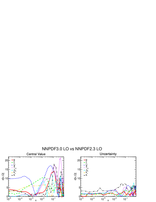
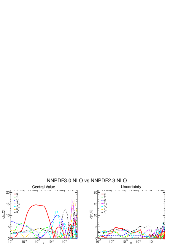
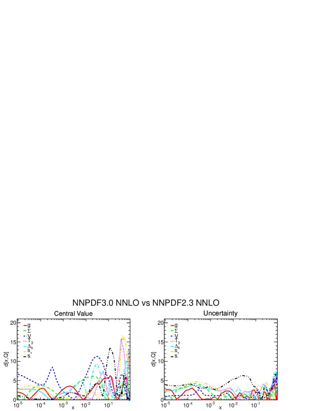
The sizes of the distances shown in Fig. 28, vary significantly with the perturbative order. At LO, the gluon in the two sets is in very good agreement for . This suggests that Monte Carlo tunes (which strongly depend on the small- gluon) based on NNPDF2.3LO, such as the Monash 2013 tune of Pythia8 [156] should also work reasonably well with NNPDF3.0LO. On the other hand, larger differences, between one and two-sigma, are found at medium and large , both for the quarks and the gluon. Note that, however, at LO theory uncertainties dominate over PDF uncertainties.
At NLO and NNLO, NNPDF2.3 and NNPDF3.0 are typically in agreement at the one-sigma level, with occasionally somewhat larger distances, of order 1.5–sigma. In particular, while the total quark singlet PDF is relatively stable, there are larger differences for individual quark flavors, especially at medium and large-. Significant differences are also found for the gluon PDF, especially at NLO, where however it should be kept in mind that NNPDF2.3 used the FONLL-A treatment of heavy quarks, while NNPDF3.0 uses FONLL-B (see Sect. 2.3.4). This comparison also shows that PDF uncertainties change at the level of one-sigma: this is to be expected, as a consequence of the constraints coming from new data, and the improved fitting methodology.
Now we turn to the direct comparison of NNPDF2.3 and NNPDF3.0 NLO PDFs: in Fig. 29 the gluon, singlet PDF, isospin triplet and total valence PDFs are shown, with at GeV2. We can see that in the NNPDF3.0 NLO set, the central value of the gluon never turns negative, even at small-: it is flat down to and then it begins to grow, within its large uncertainty, always remaining above its NNPDF2.3 counterpart. The difference can be understood as a consequence of moving to the FONLL-B heavy quark scheme, and due to the more stringent positivity constraints that are imposed now (see Sect. 3.2.3). For the total quark singlet there is good agreement between 2.3 and 3.0. For the quark triplet we see two interesting features: first at large the result in 3.0 is larger than in 2.3, especially in the region where the PDF peaks, and also the small- uncertainties are substantially larger, suggesting that they were somewhat underestimated in NNPDF2.3, presumably due to the less flexible methodology and less efficient treatment of preprocessing (see Sect. 3.2.2). As will be shown below, the small- uncertainties in the triplet between NNPDF2.3 and NNPDF3.0 become more similar when the comparison is performed in terms of 68% confidence level intervals, see Fig. 34.
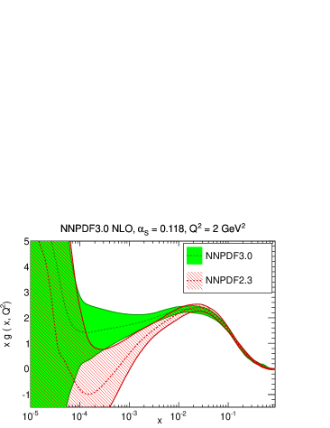

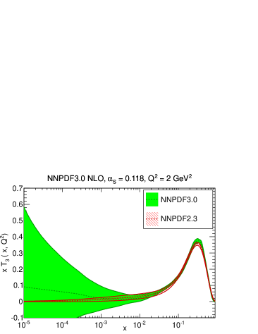
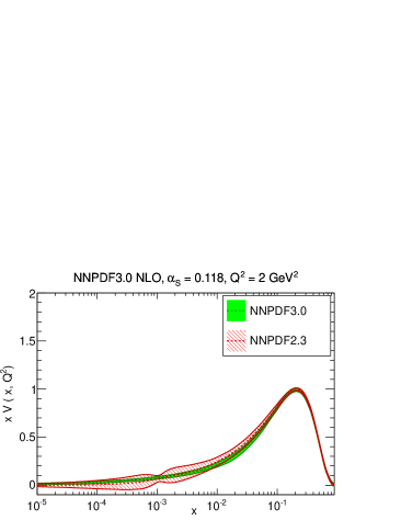
The same comparison is performed at NNLO in Fig. 30. In this case, we observe good consistency for the gluon PDF, with a reduction in the PDF uncertainties at small-. Note that in both NNLO fits the same FONLL-C GM-VFN scheme is being used. The agreement is also good for the quark singlet, as it was at NLO. For the triplet PDF , the small- uncertainties, as at NLO, are larger in 3.0 than in 2.3, though as in the case of NLO the two PDF uncertainty bands are in rather better agreement if 68% CL contours instead of one-sigma uncertainties are compared.

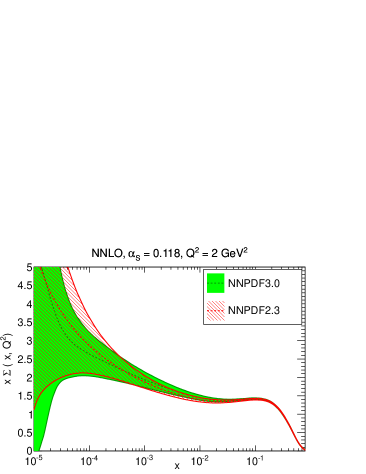
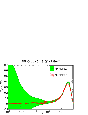
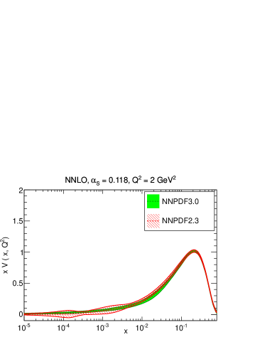
It is also interesting to compare the NNPDF2.3 and 3.0 sets at the higher scale GeV2, typical of LHC processes. Results for this comparison, at NNLO, are shown Fig. 31, as ratios to the NNPDF3.0 central value. We see that the two PDF sets agree typically at the one-sigma level or better, with some exceptions. The NNPDF3.0 gluon is somewhat softer than in NNPDF2.3, in particular in the region around which is important for the Higgs cross-section in gluon fusion. It is interesting to observe that this difference is not due to the different value of the charm mass used in NNPDF2.3 and NNPDF3.0, as the sensitivity of the gluon to the charm mass is minimal in this region, and becomes sizable only at very large ,and to a lesser extent small , where however uncertainties are very large (see Ref. [11], Fig. 40, and also Sect. 5.1.4, Fig. 41 below). The total quark singlet is also harder for , where the two error bands do not overlap, except for where the two sets agree again at one-sigma. For the triplet, there is good agreement, except near where the NNPDF2.3 and 3.0 fits disagree at the two-sigma level; for the total valence PDF there is a reasonable agreement for all values of .
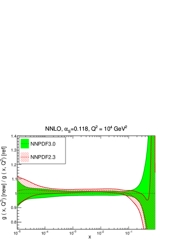
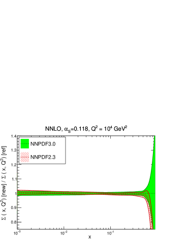
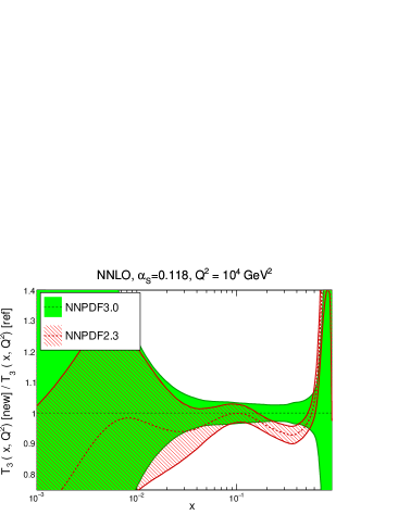
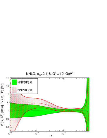
In order to assess the phenomenological impact of these changes, it is useful to look at parton luminosities. Following Ref. [157], we define the parton luminosity for the initial state as
| (35) |
where is the PDF for the -th parton, and is the invariant mass of the final state.
We compare , , and luminosities obtained using NLO and NNLO PDF sets for =13 TeV and (where for quarks a sum over light flavors is understood). The NLO and NNLO comparisons between NNPDF2.3 and NNPDF3.0 luminosities are shown in Figs. 32 and 33 respectively. At NLO, we generally find agreement at the one-sigma level, with some differences in the channel for GeV, where the error bands of the two PDF sets barely overlap, and in the channel above 1 TeV, where the luminosity is rather larger in NNPDF3.0 than in NNPDF2.3. Note that in the channel in the region around 100-200 GeV the NNPDF3.0 luminosity is somewhat softer than in NNPDF2.3, though always in agreement within PDF uncertainties.
At NNLO, in the and channels there is generally good agreement, with differences well within one sigma: for , the NNPDF3.0 luminosity tends to be larger at high invariant masses, while for around 500 GeV NNPDF3.0 is somewhat lower, with barely overlapping error bands. More significant differences are found in the channel, where the luminosity at medium invariant masses is smaller by about one sigma in NNPDF3.0 than in NNPDF2.3: in particular, for 30 GeV 300 GeV, the one sigma bands barely overlap. This has important consequences for gluon-initiated processes such as inclusive Higgs production, see Sect. 5.4.3 below. As discussed in Sect. 5.1.2, these differences stem from a combination of the improved fitting methodology and the new constraints from HERA and LHC data.
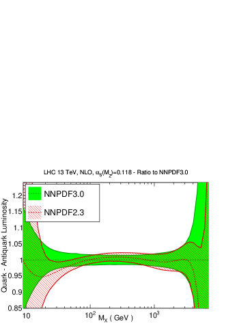
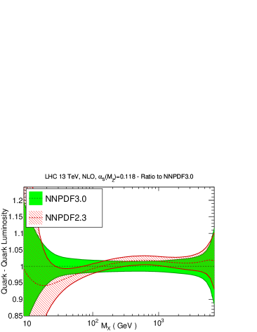
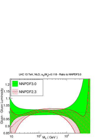

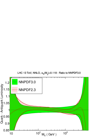


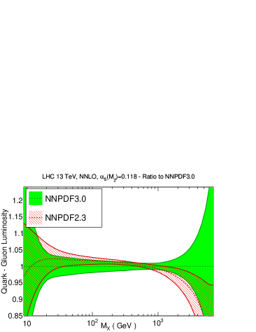
Finally, we compare one-sigma uncertainty bands to 68% confidence level intervals. For this comparison we use the NNPDF3.0 NLO fit with replicas; the conclusions would be qualitatively the same for the NNLO fit. Of course if the PDF probability distribution is Gaussian the one-sigma and 68% intervals coincide. While this is usually the case, for some PDFs in specific regions there are significant deviations from gaussianity that can be quantified by this type of comparison: typically, this happens in extrapolation regions where there are no direct experimental constraints, especially if positivity constraints, which are asymmetric, play a significant role.
This comparison is shown in Fig. 34: for most PDFs there is a good agreement, the only exception being the small- extrapolation regions, , where 68% CL intervals are typically smaller than the one-sigma bands, indicating the presence of non-gaussian outliers. For the triplet, differences are already significant for . Note that because of the generalized positivity constraints, the lower limit of 68% CL interval is typically just above zero.

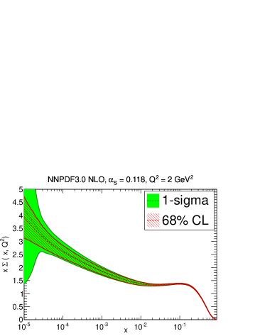
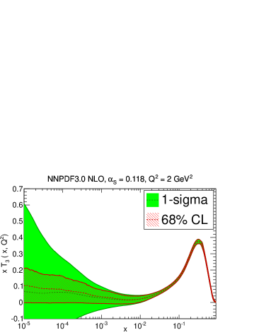
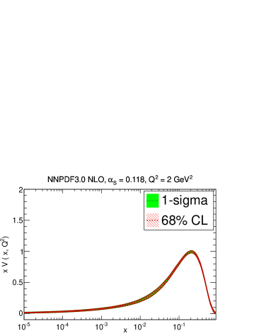
5.1.3 Perturbative stability and theoretical uncertainties
We now compare the NNPDF3.0 LO, NLO and NNLO sets: this is a meaningful comparison because the same methodology is used at all orders, with only the underlying QCD theory (and to a small extent the dataset) changing from one order to the next. In Fig. 35 we show the distances between the NNPDF3.0 pairs of fits at two consecutive orders: LO vs. NLO, and NLO vs. NNLO. In the former case, the main variation is of course seen in the gluon PDF, which as well known is very different at LO; there are also significant differences in the large- quarks. Of course, at LO theory uncertainties completely dominate over the PDF uncertainty, which depends on the data and is roughly the same at all orders, as this comparison clearly shows.
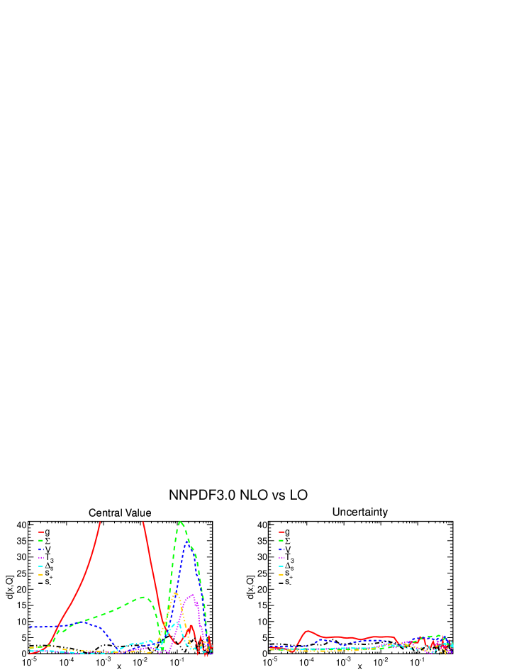
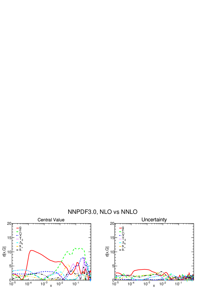
Distances become much smaller when comparing NLO to NNLO: for central values, the main differences are in the gluon PDF, both at small and at large , and in the medium- and large- quarks, in particular the total quark singlet. Uncertainties are again quite stable, with the exception on the large- gluon, where the PDF uncertainties are larger at NNLO because of the additional cuts applied to the jet data (recall Sect. 2.3.2). These differences in the fitted jet dataset also impact the central values of the two fits.
Next, in Fig. 36 we compare the LO, NLO and NNLO NNPDF3.0 parton distributions at GeV2. The large shift in the gluon between LO and NLO and its subsequent stability at NNLO is clearly seen. Specifically, the LO gluon is very large, compensating for missing NLO terms in the DIS splitting functions and anomalous dimensions. This is a crucial ingredient for the tunes to semi-hard and soft data in Monte Carlo parton shower programs (see e.g. Ref. [156]). However, in the small region missing higher order corrections cause tension between the very accurate HERA data which results in a bigger uncertainty at NLO than at LO, which then also propagates onto the singlet quark.
At NLO, the small- gluon is rather flatter than the NNLO one, which tends to go negative at small-, being prevented to do so by positivity bounds. This relatively unstable perturbative behaviour of the small- gluon might be related to unresummed small- perturbative corrections [158]. Quark PDFs are generally quite stable, with NNLO and NLO always in agreement at the one-sigma level, and sizable shifts only seen when going from LO to NLO, especially in the region around .
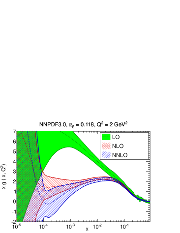
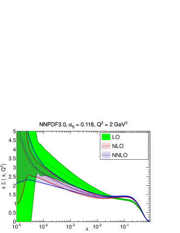
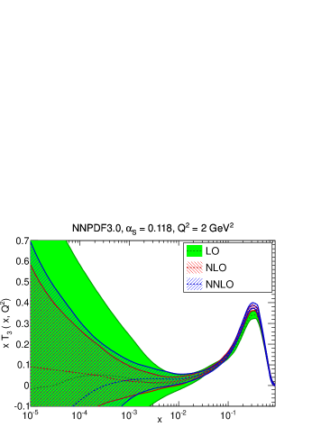
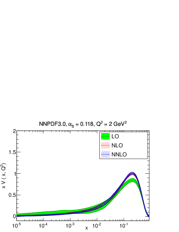
The comparison of parton distributions at different perturbative orders provides a way of estimating the uncertainty related to missing higher-order corrections in the computations used for PDF determination, using a method suggested in Refs. [159, 160] and applied to PDFs in Ref. [161]. This source of theoretical uncertainty is currently not part of the total PDF errors, which only includes uncertainties due to the data and the methodology (recall Sect. 4.3, especially Fig. 11). As these become increasingly small, however, an estimate of the theoretical uncertainty related to missing higher perturbative orders becomes more and more important.
While a full study of these uncertainties is beyond the scope of this work, we may provide a first estimate by simply studying the variation of each individual PDF when going up one order: this must be taken as an order-of-magnitude estimate for the time being, as a detailed estimate of the impact of this shift on the predictions for physical processes would involve a study of the way perturbative corrections to different processes are correlated [160, 161]. In the remainder of this section, we will refer to the uncertainty related to missing higher orders as “theory uncertainty”, while we will call PDF uncertainty the standard uncertainty as discussed on Sect. 4.3, which only includes the uncertainty from the data and the methodology.
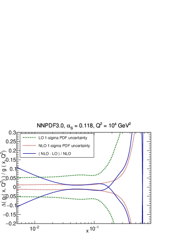
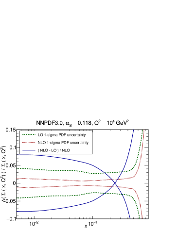
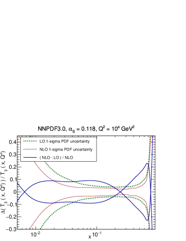
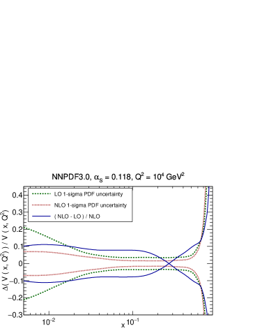
In Fig. 37 the relative shift in the central values of the NNPDF3.0 PDFs at GeV2 when going from LO to NLO (normalized to the NLO) is compared to the PDF uncertainty at the two orders. This shift may be viewed as the LO theory uncertainty, and thus likely an upper bound to the NLO theory uncertainty. It is clear that at LO theory uncertainties are dominant essentially everywhere, and especially for the small- gluon and the medium and small- quarks, as also apparent from Fig. 36.
The shifts when going from NLO to NNLO (normalized to the NNLO) are shown in Fig. 38. At this order, the theory uncertainty becomes smaller than the PDF uncertainty, thereby suggesting that their current neglect is mostly justified. However, is also apparent that theory and PDF uncertainties may become comparable in some important cases, like the large- gluon, relevant for example for top quark pair production, or the medium- quark singlet PDF, which is relevant for LHC electroweak boson production. Note that for the gluon at , relevant for Higgs production in gluon-fusion, the perturbative convergence is very good, as already highlighted in Ref. [161].
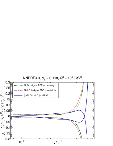
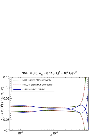
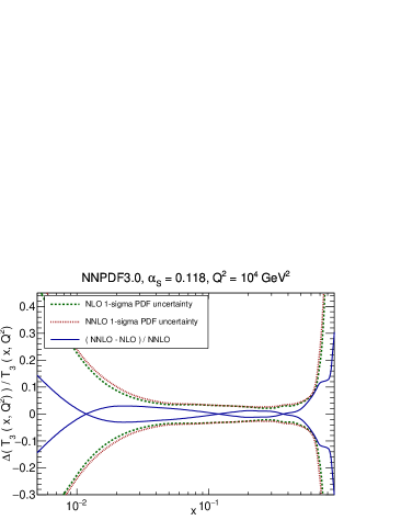
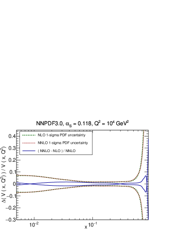
The results of Figs. 37 and 38 suggest that as PDF uncertainties decrease, either by the addition of new experimental constraints or by refinements in the fitting methodology, a careful estimate of theory uncertainties will become mandatory. In the case of NNPDF3.0 this is especially true now given that, thanks to the closure test validation, methodological uncertainties are under full control.
5.1.4 Model uncertainties
While uncertainties related to higher order corrections are perhaps the largest source of uncertainty which is not determined systematically and thus not included in the standard PDF uncertainty, there are a few more sources of uncertainty which are also not part of the current PDF uncertainty and which might become relevant as the precision of the data increases. These have to do with further approximations which are made in the theoretical description of the data, and we generically refer to them as “model” uncertainties. We now discuss the likely dominant sources of model uncertainties, namely, those related to nuclear corrections and those related to the treatment of heavy quarks.
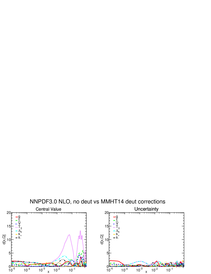
Several fixed-target data included in the NNPDF3.0 PDF determination are taken on nuclear targets. These include all of the neutrino deep-inelastic scattering data, namely the CHORUS and NuTeV data sets of Table 1, the data for charged-lepton deep-inelastic scattering from deuteron targets in the NMC, BCDMS, and SLAC data sets also in Tab. 1, and the data for Drell-Yan production on a deuterium target in the DY E866 data set in Tab. 2. The impact of nuclear corrections on the NNPDF2.3 PDF determination was previously discussed in Ref. [103], where the NNPDF2.3 fit was repeated by introducing deuterium nuclear corrections according to various models, and found to be non-negligible (up to about one and a half sigma) but effecting only the down distribution at large .
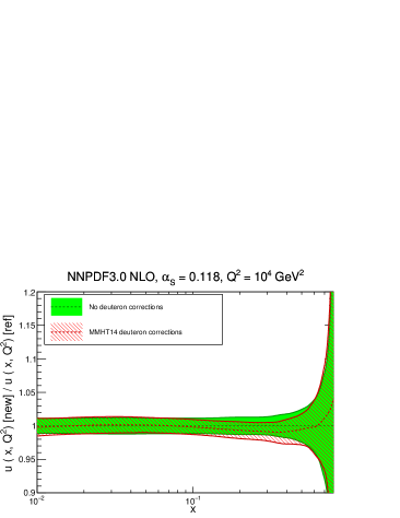
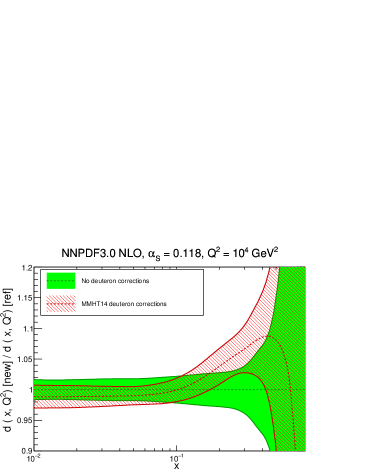
We have repeated the NNPDF3.0 PDF determination, but now including deuterium corrections according to the recent model of Ref. [162], which supersedes the previous treatment of higher twist corrections of Ref. [163], considered in Ref. [103] along with other models. The pattern of deviations between the PDFs determined with and without nuclear correction is shown in Fig. 39, and it is very similar to that seen in Ref. [103] when correcting the NNPDF2.3 in an analogous way, but with a somewhat more moderate impact, as one might expect given the fact that the data set used to determine NNPDF3.0 is bigger than that used for NNPDF2.3. Essentially only the up and down quark distributions are affected; they are compared in Fig. 40, at GeV2: it is apparent that the effect is always below one sigma. In view of the theoretical uncertainty involved in the modeling of these corrections, we prefer not to include them in the fit as it is unclear that the uncertainty on them is significantly smaller than their size. Nuclear corrections to neutrino data are likely to be yet smaller, with the possible exception of the strange distribution [162].
Another important potential source of theoretical uncertainty is related to the treatment of heavy quarks. As discussed in Sect. 2.3.4, we use a computational scheme, the FONLL scheme, which ensures that all the available perturbative information is included. However, there are also aspects that go beyond perturbation theory, namely, the dependence on the quark mass itself, and the possible presence of an intrinsic heavy quark component [164], namely, the possibility that the boundary condition for the evolution of the heavy quark PDFs is not zero, but rather an independently parametrized PDF [165].
The dependence of PDFs on the values of the heavy quark masses was previously studied by us in Ref. [11] within the context of the NNPDF2.1 PDF determination, where the values of and were varied, in the absence of intrinsic heavy quark PDFs. The main result of this study was that the value of the heavy quark mass mostly affects the heavy quark PDF by providing the threshold for generating it by perturbative evolution: a lower mass value corresponds to a larger PDF at a given scale, because the evolution length is larger. For the quark PDFs, which are expected to be perturbative quantities, with a negligible intrinsic component, this dependence on the quark mass value is likely to be a real physical effect. However since charm has a threshold at the boundary between the perturbative and nonperturbative regions, charm PDFs might have a significant intrinsic component, and much of the dependence on the charm mass might be compensated by changes in this intrinsic PDF.
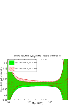
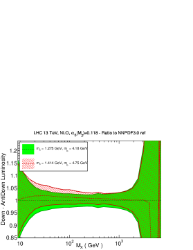
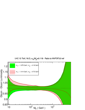
As mentioned in Sect. 2.3.4, Eq. 2, the heavy quark mass values used in the current NNPDF3.0 PDF determination differ from the values previously used in the NNPDF 2.3 determination, essentially because now we use PDG mass values, while the previous values were close to pole mass values. The shift is larger than the current uncertainty on masses. In order to assess the impact of this change, and thus also of the dependence on heavy quark masses, we have repeated the NNPDF3.0 PDF NLO determination using the heavy quark mass values that were used for the NNPDF2.3 set. In Fig. 41 the respective parton luminosities at GeV2 are compared.
Results are in agreement with the findings of Ref. [11], where a similar effect due to changes of the charm mass was observed. Note that the impact of changing the bottom mass was found to be negligible on all luminosities, except the bottom luminosity itself. The effect is not entirely negligible. However, as mentioned above, we expect that some of this dependence might be absorbed into an intrinsic charm PDF. At NLO, and pole mass-scheme expressions coincide, with a small correction at NNLO, hence it seems more appropriate to use the more accurate mass value. The shifts seen in Fig. 41 should be taken as an upper bound to the size of the uncertainty related to the charm mass value, whose exact assessment will only be possible once an intrinsic charm component is introduced in our PDF fits.
We finally mention that further model uncertainties are expected to come from the treatment of electroweak interactions, both in the choice of parameters, and the treatment of higher order terms (including mixed strong-electroweak corrections [166]). These are generally smaller than the uncertainties discussed here, though they could become significant in particular kinematic regions or for specific processes, such as for instance high-mass production of pairs.
5.2 Dependence on the dataset
We now study the dependence of the NNPDF3.0 PDFs on the choice of dataset, exploring a wide range of variations as compared to the dataset used in the reference global fit. First, we propose a new definition of conservative PDFs based on a maximally consistent dataset, along the lines of previous proposals [167], but now using an objective criterion, rather than theoretical expectations. Then we explore systematically the impact of the new data in the NNPDF3.0 framework, by comparing fits to various subsets of data both to the global fit, and to a minimal fit based on HERA data only; in this context we also study the impact of the new HERA-II data. We also construct sets where the HERA data is supplemented by all available data by either ATLAS or CMS; these are specially useful for comparisons with related studies by the LHC collaborations. We specifically study in detail the impact of jet data, the associate theoretical uncertainties, and their impact on the uncertainty on the large- gluon, and the impact of + data on strangeness and their relative weight in comparison to neutrino data.
5.2.1 Conservative PDFs from a consistent dataset
Inconsistencies between data which enter a global PDF determination can distort the statistical interpretation of PDF uncertainties. Inconsistency of any individual dataset with the bulk of the global fit may suggest that its understanding, either from the theoretical or experimental point of view, is not complete, and that its exclusion from the fit might be advantageous. In order to minimize such inconsistencies, “conservative” partons have been suggested, for example by introducing restrictive kinematic cuts which remove potentially dangerous regions [167], or by picking data which one might expect to be more reliable: for example, the NNPDF2.3 collider-only fit [13], based on the expectation that collider data, because of their higher energy, should be more reliable than fixed-target data.
| NLO global fit | NNLO global fit | |||||
| Experiment | mean | mode | median | mean | mode | median |
| NMC | 1.04 | 1.01 | 1.03 | 1.04 | 1.01 | 1.03 |
| NMC | 1.32 | 1.31 | 1.27 | 1.27 | 1.26 | 1.27 |
| SLAC | 1.31 | 1.27 | 1.30 | 1.13 | 1.09 | 1.12 |
| BCDMS | 1.17 | 1.16 | 1.17 | 1.20 | 1.19 | 1.20 |
| CHORUS | 1.11 | 1.10 | 1.11 | 1.10 | 1.09 | 1.09 |
| NuTeV | 1.04 | 0.90 | 0.98 | 1.06 | 0.92 | 1.00 |
| HERA-I | 1.09 | 1.09 | 1.10 | 1.10 | 1.09 | 1.09 |
| ZEUS HERA-II | 1.23 | 1.22 | 1.23 | 1.25 | 1.24 | 1.25 |
| H1 HERA-II | 1.30 | 1.3 | 1.31 | 1.35 | 1.34 | 1.34 |
| HERA | 1.10 | 1.06 | 1.09 | 1.14 | 1.11 | 1.13 |
| E886 | 1.00 | 0.88 | 0.96 | 1.01 | 0.88 | 0.96 |
| E886 | 1.13 | 1.11 | 1.12 | 1.15 | 1.14 | 1.15 |
| E605 | 0.97 | 0.94 | 0.96 | 0.94 | 0.91 | 0.93 |
| CDF rapidity | 1.34 | 1.28 | 1.32 | 1.39 | 1.32 | 1.36 |
| CDF Run-II jets | 1.09 | 1.06 | 1.08 | 1.15 | 1.12 | 1.14 |
| D0 rapidity | 1.34 | 1.28 | 1.32 | 0.86 | 0.82 | 0.85 |
| ATLAS 2010 | 1.20 | 1.15 | 1.18 | 1.17 | 1.12 | 1.15 |
| ATLAS 7 TeV jets 2010 | 0.76 | 0.74 | 0.75 | 1.09 | 0.92 | 1.02 |
| ATLAS 2.76 TeV jets | 0.86 | 0.83 | 0.85 | 1.07 | 0.57 | 0.83 |
| ATLAS high-mass DY | 2.22 | 1.68 | 2.03 | 1.82 | 1.34 | 1.63 |
| CMS electron asy | 1.05 | 0.91 | 0.99 | 1.00 | 0.87 | 0.95 |
| CMS muon asy | 1.62 | 1.42 | 1.54 | 1.60 | 1.40 | 1.53 |
| CMS jets 2011 | 1.01 | 0.97 | 0.99 | 1.09 | 1.07 | 1.08 |
| CMS + total | 1.60 | 1.17 | 1.42 | 1.50 | 1.09 | 1.33 |
| CMS + ratio | 1.93 | 1.43 | 1.74 | 1.88 | 1.39 | 1.69 |
| CMS 2D DY 2011 | 1.27 | 1.25 | 1.27 | 1.28 | 1.27 | 1.28 |
| LHCb rapidity | 1.10 | 1.02 | 1.07 | 1.20 | 1.12 | 1.17 |
| 1.65 | 1.24 | 1.49 | 1.09 | 0.75 | 0.95 | |
| Global fit | ||||||||
|---|---|---|---|---|---|---|---|---|
| Total | 0.96 | 1.01 | 1.06 | 1.10 | 1.12 | 1.16 | 1.23 | 1.29 |
| NMC | 0.91 | 0.91 | 0.89 | 0.89 | 0.88 | 0.89 | 0.92 | 0.93 |
| NMC | - | - | - | - | - | - | 1.63 | 1.52 |
| SLAC | - | - | - | - | 1.77 | 1.19 | 1.59 | 1.13 |
| BCDMS | - | - | 1.11 | 1.15 | 1.12 | 1.16 | 1.22 | 1.29 |
| CHORUS | - | - | 1.06 | 1.02 | 1.09 | 1.07 | 1.11 | 1.09 |
| NuTeV | 0.35 | 0.34 | 0.62 | 0.64 | 0.70 | 0.70 | 0.70 | 0.86 |
| HERA-I | 0.97 | 0.98 | 1.02 | 1.00 | 1.02 | 0.99 | 1.05 | 1.04 |
| ZEUS HERA-II | - | - | - | - | 1.41 | 1.48 | 1.40 | 1.48 |
| H1 HERA-II | - | - | - | - | - | - | 1.65 | 1.79 |
| HERA | - | - | 1.21 | 1.32 | 1.20 | 1.31 | 1.27 | 1.28 |
| E886 | 0.30 | 0.30 | 0.43 | 0.40 | 0.44 | 0.46 | 0.53 | 0.48 |
| E886 | - | - | 1.18 | 1.40 | 1.27 | 1.53 | 1.19 | 1.55 |
| E605 | 1.04 | 1.10 | 0.74 | 0.83 | 0.75 | 0.88 | 0.78 | 0.90 |
| CDF rapidity | - | - | - | - | - | - | 1.33 | 1.53 |
| CDF Run-II jets | - | - | 1.01 | 2.01 | 1.04 | 1.84 | 0.96 | 1.80 |
| D0 rapidity | 0.56 | 0.61 | 0.62 | 0.71 | 0.60 | 0.69 | 0.57 | 0.61 |
| ATLAS 2010 | - | - | 1.19 | 1.13 | 1.19 | 1.17 | 1.19 | 1.23 |
| ATLAS 7 TeV jets 2010 | 0.96 | 1.65 | 1.08 | 1.58 | 1.10 | 1.54 | 1.07 | 1.36 |
| ATLAS 2.76 TeV jets | 1.03 | 0.38 | 1.38 | 0.36 | 1.35 | 0.35 | 1.29 | 0.33 |
| ATLAS high-mass DY | - | - | - | - | - | - | 2.06 | 1.45 |
| ATLAS | - | - | - | - | - | - | 1.13 | - |
| CMS electron asy | 0.98 | 0.84 | 0.82 | 0.72 | 0.85 | 0.73 | 0.87 | 0.73 |
| CMS muon asy | - | - | - | - | - | - | 1.81 | 1.72 |
| CMS jets 2011 | 0.90 | 2.09 | 0.96 | 2.09 | 0.99 | 2.10 | 0.96 | 1.90 |
| CMS total | - | - | - | - | - | - | 0.96 | 0.84 |
| CMS ratio | - | - | - | - | - | - | 2.02 | 1.77 |
| CMS 2D DY 2011 | - | - | - | - | 1.20 | 1.30 | 1.23 | 1.36 |
| LHCb rapidity | - | - | 0.69 | 0.65 | 0.74 | 0.69 | 0.71 | 0.72 |
| LHCb rapidity | - | - | 1.23 | 1.78 | 1.11 | 1.58 | 1.10 | 1.59 |
| - | - | - | - | - | - | 1.43 | 0.66 | |
We propose a new objective definition of a conservative set of PDFs based on a measure of consistency between datasets introduced in Ref. [18, 154]. This is based on observing that lack of compatibility can always be viewed as an underestimate of the covariance matrix: if the covariance matrix is inflated by a factor , then compatibility can always be attained if if large enough (crudely speaking, if uncertainties are all multiplied by a factor ). It is then possible to measure compatibility by assuming that the prior knowledge is given by all experiments in the global dataset but the given one, and using Bayes’ theorem to study how this prior is modified when adding the experiment whose consistency is under investigation. One may then compute the a posteriori probability that the covariance matrix of the given experiment should be rescaled by a factor . Compatibility corresponds to the case in which peaks around , while if the most likely value is at , this means that compatibility is only achieved when uncertainties are inflated by (see Ref. [18, 154] for a more detailed discussion and definition). The definition of the , which is used for minimization (see Sect. 5.1.1), is also used in the determination of .
We then proceed as follows. We compute the probability distribution of the rescaling variable , for each dataset included in the global fit, and we determine the mean, the median and the mode of the corresponding distribution. We then exclude from the conservative fit all experiments for which at least two of these three quantities are above some threshold value, denoted by . We discard all datasets for which the criterion fails either at NLO or at NNLO (or both), which corresponds to the most conservative choice of only retaining experiments which are well described at all perturbative orders, and has the obvious advantage that the dataset does not depend on the perturbative order, thereby keeping PDF uncertainties separate from the theory uncertainties discussed in Sect. 5.1.3. In practice, for simplicity we compute the probability without excluding the given experiment from the global fit: this provides a conservative estimate of the compatibility (which is clearly increased by including the experiment under investigation in the prior) without requiring us to construct a new set of 1000 replicas when each of the experiments is excluded in turn. The values of the mean, median and mode thus computed for all the experiments in the NNPDF3.0 global fits at NLO and NNLO are collected in Tab. 10.222We notice that the ATLAS data, which are included in the NNPDF3.0 global fit, are not included in Tab. 12. This is due to the fact the we construct NLO and NNLO conservative PDF sets s based on the same datasets. Since the ATLAS data are excluded from the global NNLO fit because of the lack of availability of a NNLO prediction, they will not be included in our conservative set.
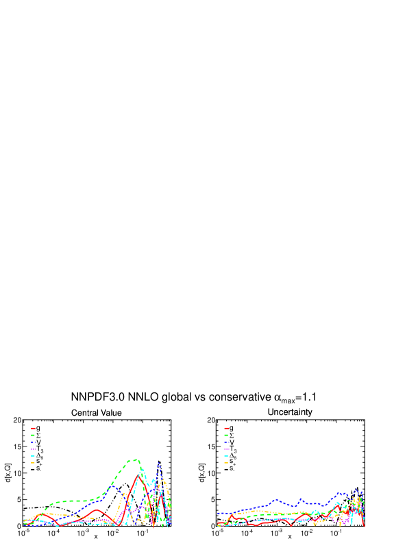
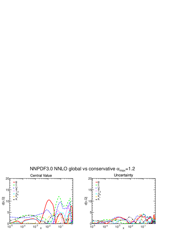
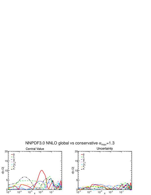
In the following we present results for partons obtained by fitting to datasets constructed by only including data from Tab. 10 which pass the conservative cuts corresponding to three different values of , namely 1.1, 1.2 and 1.3. In Tab. 11 we provide the (for ease of comparison we show results obtained using the experimental definition, see Sect. 5.1.1) for the PDF fits to these datasets. To facilitate the comparison with the global fit, we also provide its values in the same table, taken from Tab. 9.
| NNLO global fit | NNLO cons. fit | |||||
| Experiment | mean | mode | median | mean | mode | median |
| NMC | 1.27 | 1.26 | 1.27 | 1.50 | 1.45 | 1.48 |
| SLAC | 1.13 | 1.09 | 1.12 | 1.61 | 1.37 | 1.48 |
| BCDMS | 1.20 | 1.19 | 1.20 | 2.02 | 1.86 | 1.92 |
| CHORUS | 1.10 | 1.09 | 1.09 | 2.55 | 1.69 | 2.32 |
| ZEUS HERA-II | 1.25 | 1.24 | 1.25 | 1.38 | 1.33 | 1.36 |
| H1 HERA-II | 1.35 | 1.34 | 1.34 | 1.51 | 1.47 | 1.49 |
| HERA | 1.14 | 1.11 | 1.13 | 1.13 | 1.09 | 1.12 |
| E886 | 1.15 | 1.14 | 1.15 | 2.18 | 1.62 | 2.03 |
| CDF rapidity | 1.39 | 1.32 | 1.36 | 1.56 | 1.40 | 1.50 |
| CDF Run-II jets | 1.15 | 1.12 | 1.14 | 1.25 | 1.18 | 1.22 |
| ATLAS 2010 | 1.17 | 1.12 | 1.15 | 1.38 | 1.25 | 1.32 |
| ATLAS high-mass DY | 1.00 | 1.34 | 1.63 | 1.63 | 1.19 | 1.45 |
| CMS muon asy | 1.60 | 1.40 | 1.53 | 2.90 | 2.48 | 2.81 |
| CMS + total | 1.50 | 1.09 | 1.33 | 1.85 | 1.37 | 1.67 |
| CMS + ratio | 2.00 | 1.39 | 1.69 | 2.12 | 1.58 | 1.94 |
| CMS 2D DY 2011 | 1.28 | 1.27 | 1.28 | 1.29 | 1.28 | 1.29 |
| LHCb | 1.20 | 1.12 | 1.17 | 1.58 | 1.22 | 1.48 |
The improvement in global fit quality as is lowered is apparent, with the most conservative option leading to an essentially perfect of order one. It is interesting to observe that NMC proton data, which are known to have internal inconsistencies [3], as well as other datasets such as the H1 HERA-II data, the ATLAS high-mass Drell-Yan data, and the CMS + data are excluded even from the least conservative set, the one with . On the other hand, the CMS inclusive jet data is included for all values of ; note that for this dataset the experimental shown in Tab. 11 is significantly worse than the value used for minimization and the determination of .
The maximally consistent dataset, found with , includes the NMC data, the NuTeV and HERA-I DIS data, the Drell-Yan data from E866 and E605, the D0 Z rapidity, the ATLAS and CMS inclusive jets and the CMS electron asymmetry.
In Tab. 12, we furthermore compare the mean, mode and median of the distributions for the experiments excluded from the NNLO conservative fit with when the global fit is used as prior (i.e. the same numbers for the corresponding entries in Tab. 10), to the same quantities computed using as a prior the conservative fit itself. All the peak values of deteriorate when using the conservative set as a prior, as they ought to. Clearly, this deterioration will be maximal for datasets which are internally consistent, but inconsistent with the rest, and more moderate for experiments which are affected by internal inconsistencies, so that a rescaling of uncertainties is needed in order to describe them, regardless of what one takes as a prior. This is the case for instance for the NMC which are affected by internal inconsistencies as already mentioned.
The distance between the conservative sets and the baseline NNPDF3.0 NNLO global fit are show in Fig. 42, while PDFs are compared directly at GeV2 in Fig. 43, where the NNLO conservative fits with and 1.2 and the reference fit are shown, and at GeV2 in Fig. 44, where the NNLO conservative fit with is shown as a ratio to the default global fit. All sets are consistent with the global fit, with PDFs that differ at most at the one-sigma level, thereby confirming the consistency of the procedure, though of course PDF uncertainties are larger in the fits to reduced datasets. The small- gluon is similar in all cases because is driven by the HERA-I data, while there is more dependence on the choice of at medium and large : interestingly, in the region relevant for Higgs production in gluon fusion the gluon is significantly affected by the choice of , though not beyond the one-sigma level. The quarks are also in good agreement, with the main differences seen at medium . The set with has of course the largest PDF uncertainties, though even with the correspondingly restricted dataset of Tab. 11 they are not much worse than those of the global fit, with the valence and triplet, and thus the quark-antiquark flavor separation becoming rather more uncertain.
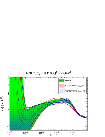
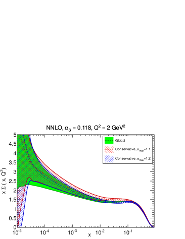
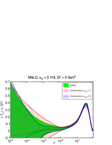
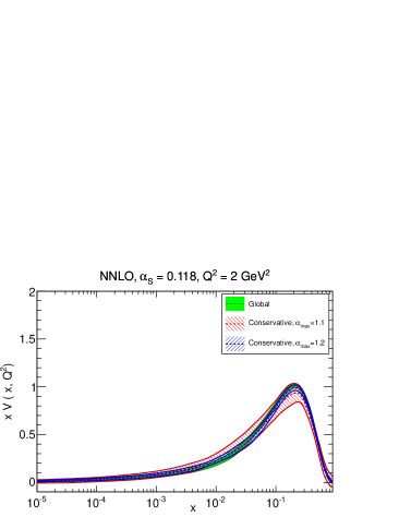

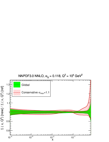
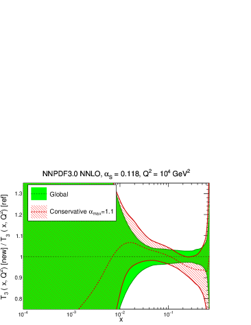
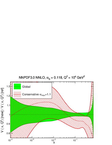
These conservative parton sets may be used for studies aimed at assessing how individual datasets affect LHC observables, by studying their effect on a maximally self-consistent dataset, such as performed in Ref. [168]. In the future, as more and more data will become available, this approach might also be used in deciding for an optimal dataset on which a global fit should be based.
5.2.2 Impact of the new HERA and LHC data
We now examine in detail the impact of the new HERA and LHC data in NNPDF3.0. Results will be shown for NNLO fits, by investigating the impact of the new data both on the global fit, and also on a HERA-only fit: while the former is more realistic, the latter allows for an assessment of the specific impact of each individual piece of data (though of course it over-estimates their impact in a realistic setting). Jet data will be specifically discussed in Sect. 5.2.3 below. In all these fits, exactly the same theory and the same methodology of the default set will be used, with only the dataset changing, so that the impact of the dataset is specifically assessed. This will eventually allow us to provide a quantitative assessment of the dependence on the dataset of the uncertainty on our prediction.
In order to have a first overall assessment, we have produced a variant of the NNPDF3.0 fit using the same methodology, but using an NNPDF2.3-like dataset. We include in the dataset for this fit all, and only, the data from Tables 1-2 which were included in the NNPDF2.3 dataset. This is not quite identical to the NNPDF2.3 dataset, because we include these data with the same cuts as in NNPDF3.0 (which are sometimes slightly different than those of NNPDF2.3, as discussed in Sect. 2) and not the data of Tables 3, despite the fact that these were included in NNPDF2.3. It is however adequate to assess the (moderate) impact of the new data as we now see.
The distances between PDFs from this fit and their NNPDF3.0 counterparts are shown in Fig. 45, while the PDFs at are compared in Fig. 46. Is clear that the new data affects moderately all PDFs: central values vary within half a sigma of the PDF errors at most. This was to be expected, since the NNPDF2.3 PDFs already described rather well all the new experimental data that has been added in NNPDF3.0, so the main impact of the new data is to reduce uncertainties. Indeed, the PDF comparison shows that the change in uncertainties, seen in the distance plot again at a half-sigma level, always corresponds to a reduction in uncertainty.


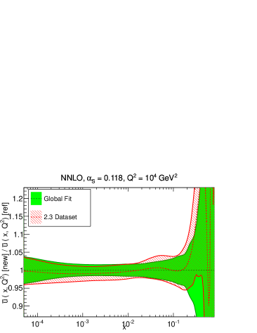
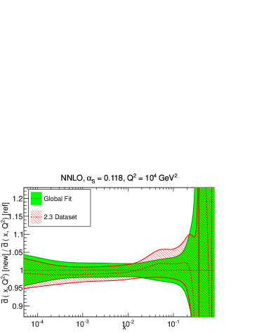
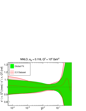
The largest effect on central values is seen for the large- and medium- quarks, followed by the gluon in the same region. The small- gluons and quarks are quite stable since there is no new data that affects them in this region. Uncertainties mostly improve for the gluon PDF, both at large thanks to the LHC jet and top quark data, and at medium and small from the new HERA-II data. The new data favor a rather softer gluon at large in comparison to the NNPDF2.3-like dataset, though differences are always within the PDF uncertainties. Also for the antiquark sea there is a visible improvement, especially at medium , where the bulk of the LHC electroweak vector boson production data is. Finally, there are some improvements in strangeness; the role of the LHC data in pinning down is discussed in more detail in Sect. 5.2.4.
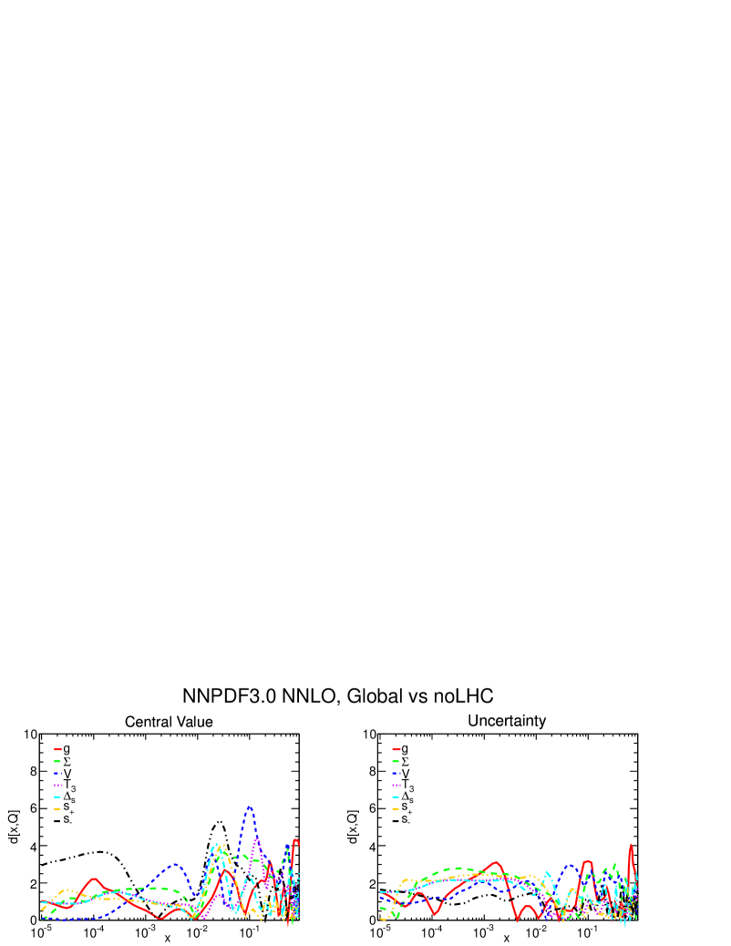
We now focus specifically on the impact of LHC data: to this purpose, we produce a fit excluding all the LHC data from the dataset, including those which were already in NNPDF2.3, and keeping all the other data in the NNPDF3.0 fit (including the HERA-II data). The corresponding distances are shown in Fig. 47, while PDFs are compared in Fig. 48.
The impact is seen to be moderate, at a half-sigma level, both for central values and for uncertainties, but it always leads to an improvement in uncertainties. Central values are mostly affected for quarks at medium and large , at to a lesser extent for the gluon.
Reassuringly, PDFs without LHC data are always within the one sigma uncertainty bands of the global fit PDFs, confirming the consistency of LHC data with the previous dataset. The gluon at medium and small is already well constrained by HERA and Tevatron data, but the LHC improves uncertainties for , thanks to the ATLAS and CMS inclusive jet data and top quark production data. The down quark and strange PDFs are also affected, especially in the small- region, but also at medium .
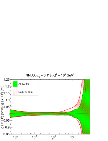
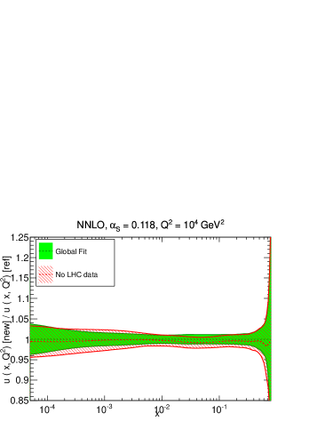

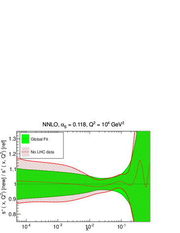
Next, we construct a PDF set based on HERA data only. This is then used to further assess the impact of the ATLAS and CMS data. These HERA-only PDFs are compared to the global fit at GeV2 in Fig. 49. Clearly, most PDFs, with the partial exception of the small- gluon, have much larger uncertainties than the global fit: specifically, the quark flavor separation and the large- gluon are very poorly constrained in a HERA-only fit, which is thus not competitive with a global fit for phenomenology applications.

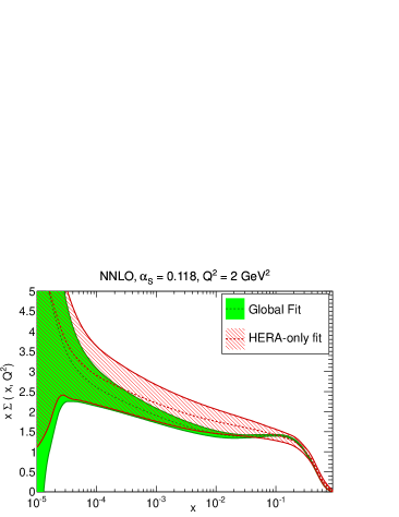
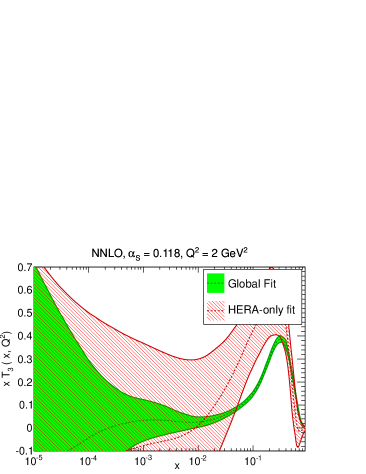
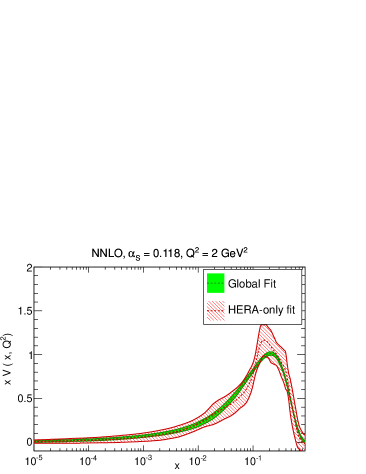
The HERA dataset has widened considerably with the addition of the complete HERA-II inclusive data from H1 and ZEUS and combined HERA charm production data. In order to study the impact of this data, we have produced a version of the HERA-only fit in which we have kept only the combined HERA-I data, i.e. a HERA-I-only fit. The NNLO PDFs of the HERA-only and HERA-I-only fits are compared at GeV2 in Fig. 50. The additional information provided by HERA-II apparently has a moderate impact: the gluon is mostly unchanged, while the PDF uncertainties on the medium- and large- up antiquarks and (to a lesser extent) on the down antiquarks are moderately reduced. We conclude that, while certainly beneficial, the new HERA-II data does not change substantially the known fact that HERA-only fits are affected by large PDF uncertainties.
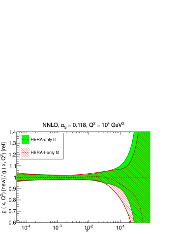
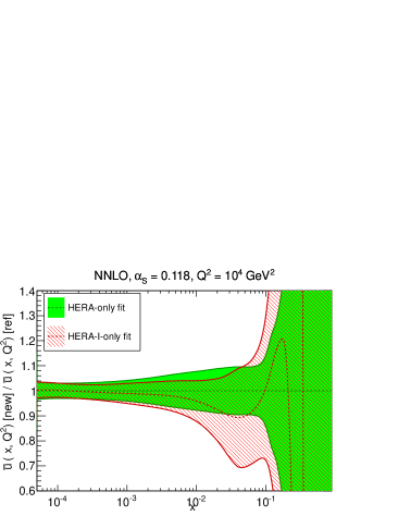

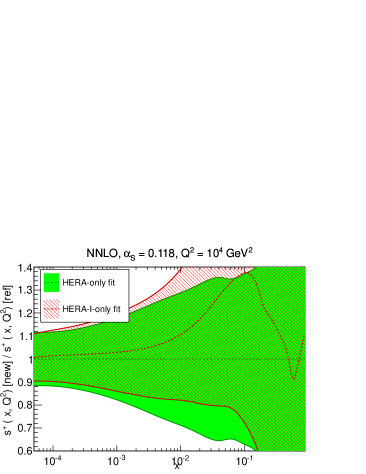
We now study the response of HERA-only fit of Fig. 43 upon addition of various pieces of data. In particular, we produce two fits, respectively from a dataset obtained by adding to the HERA data all the ATLAS data or all the CMS data. Specifically (see Tab. 1) in the HERA+CMS fit, the HERA data is supplemented with data on jet production, asymmetries, Drell-Yan differential distributions, + production and top quark total cross-sections, while in the HERA+ATLAS fit, the HERA measurements are supplemented with rapidity distributions from the 2010 dataset, inclusive jet data at 7 TeV and 2.76 TeV, and high-mass Drell-Yan production.
The distances between the HERA-only and HERA+ATLAS, or HERA-only vs. HERA+CMS fits are shown in Fig. 51, while the gluon and PDFs are shown in Fig. 52, with the default global fit also shown for reference. The impact of the LHC data is now apparent, in particular for PDF combinations which are poorly constrained by a fit to HERA data only, specifically the large- gluon and the the quark flavor separation. Note that the CMS data provides more stringent constraints on the gluon at large since it uses the 2011 inclusive jet data, which for ATLAS is still not available. ATLAS and CMS have a similar constraining power for the medium and large- quarks, with CMS slightly superior for the strangeness PDFs thanks to the availability of the + measurements, and also for flavor separation (and thus for ) due to the fact that the CMS electroweak dataset is somewhat more extensive.
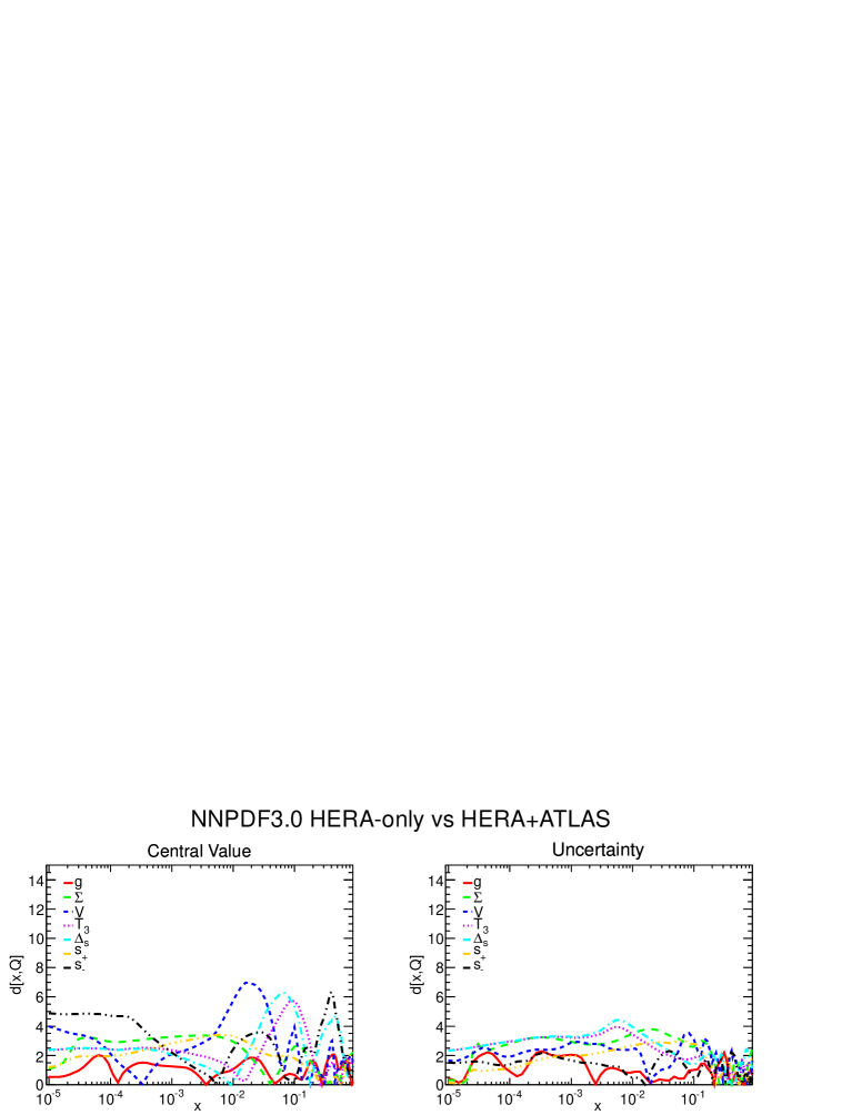

On the other hand, comparison to the global fit shows that neither of these HERA+ATLAS or HERA+CMS fits is yet competitive. Also, comparison of these result to our previous assessment of the overall impact of LHC data on the global fit (Figs. 47 and 48) shows that gauging the impact of LHC data on PDFs by their effect on a HERA-only fit might be somewhat misleading: because of the good consistency of LHC data with the pre-LHC global dataset, their impact in the global fit is rather less pronounced.

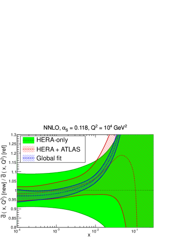
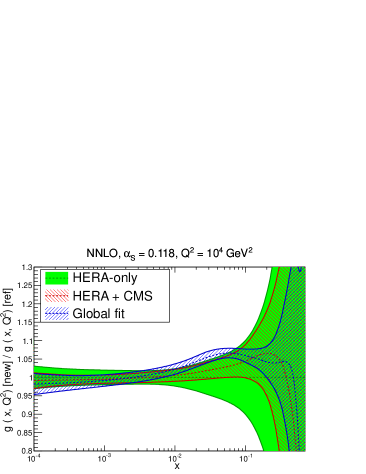
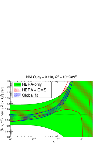
We finally come to a global assessment of the dependence of the PDF uncertainty on the dataset. This can be done by using the estimator , Eq. (24), which, as discussed in Sect. 4, is essentially the ratio of the PDF uncertainty on the prediction to the original experimental uncertainties, averaged over all data, and keeping into account all correlations. Its value thus measures by how much the data uncertainty, propagated to the PDFs, and then propagated back to the data, is reduced due to the fact that the PDF fits combines many data points into a single set of PDFs which are constrained both by theory (such as perturbative evolution, which connects different values of , and sum rules, which relates different values of ) and also by smoothness (the value of any PDF at neighboring points in cannot differ by an arbitrarily large amount). For a single data point, or if data points were independent, its value would be one by definition, while its deviation from one estimates the uncertainty reduction (or increase, which could happen in principle when combining inconsistent data). Note that this indicator only probes the PDF uncertainty at the data points: so the reduction in uncertainty when widening the dataset is actually somewhat underestimated by it, in that for a bigger dataset the given value of actually refers to a wider kinematic region.
In Tab. 13 we show for the global NNPDF3.0 NLO and NNLO fits, as well as for the fits based on reduced datasets, starting from the HERA-I only fit and including the fit without LHC data, in increasing order of the size of the fitted dataset. The result for the conservative set refers to the fit with threshold .
For the global fits, we find and 0.302 for the NLO and NNLO sets respectively, to be compared with the corresponding value at LO, . The improvement between LO and NLO, almost by a factor of two in terms of the reduction of the PDF uncertainties to the fitted data points, is clear evidence of the better consistency of the NLO fit in comparison to the LO one. On the other hand, the NNLO fit is very similar to the NLO one in this respect (perhaps marginally worse), consistent with the observation that the quality of the NNLO fit is not better than that of the NLO fit, as also measured by the value of the , see Tab. 9.
The monotonic decrease of the values of for the fits to reduced datasets, from HERA-I to HERA-all, to HERA+ATLAS or HERA+CMS, to the global fit, shows the constant uncertainty reduction as more data are combined. The uncertainty on the conservative fit is larger than that of any fit except the HERA-I fit. This provides evidence in favor of using our current default as reference, rather than the conservative set, as the substantial decrease in in the global fit in comparison to the conservative one suggests that the overall consistency of the global fit is still quite good. Finally, the uncertainty on the no-LHC fit is larger than that of a global fit, and in fact comparable to that of the HERA+CMS fit: this shows that even though the impact of the LHC data is moderate, it is visible, and it is comparable to the impact of all the other non-HERA data.
| Dataset | NLO | NNLO |
|---|---|---|
| Global | 0.291 | 0.302 |
| HERA-I | 0.453 | 0.439 |
| HERA all | 0.375 | 0.343 |
| HERA+ATLAS | 0.391 | 0.318 |
| HERA+CMS | 0.315 | 0.345 |
| Conservative | 0.422 | 0.478 |
| no LHC | 0.312 | 0.316 |
5.2.3 Impact of jet data on the global fit
We now explore the impact of jet data in the NLO and NNLO NNPDF3.0 fits, with the motivation of making sure that theoretical limitations in the description of jet data, and in particular the current lack of full knowledge of NNLO corrections, does not bias the fit results.
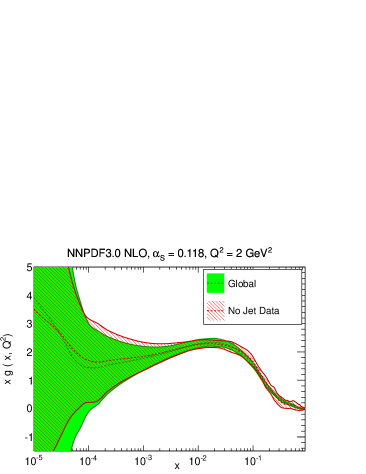
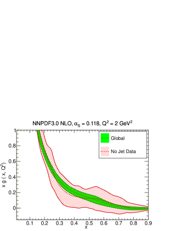
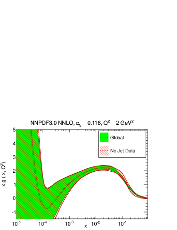
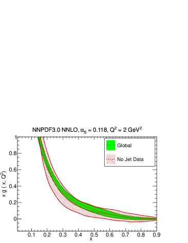
To this purpose, we have produced versions of the NNPDF3.0 PDF fit in which all jet data are removed from the global dataset: the gluon from these sets is compared to that from the default global fit at GeV2 in Fig. 53: Other PDFs are essentially unchanged upon removing jet data. It is clear that removing jet data from the global fit leads to a substantial increase of the PDF uncertainties on the gluon at medium- and large-. However, when jet data are included, the uncertainties are very similar at NLO and NNLO, despite the fact that at NNLO the jet dataset is significantly smaller due to the more restrictive cuts which we have introduced in order to account for the incomplete knowledge of NNLO corrections to jet production (see Sect. 2.3.2): in fact, if anything, the uncertainties are somewhat smaller at NNLO. This is reassuring in that it is consistent with the expectation that no instabilities are introduced by jet data in the NNLO fit despite potentially large perturbative corrections, and in fact the fit becomes tighter at NNLO.
In Tab. 14 we compare at NLO and NNLO the to the collider jet data, both in the reference NNPDF3.0 fit and in the fit without jet data. We provide the results using both the experimental and the definitions, whose values can differ significantly, especially at NNLO. The description of jet data turns out to be reasonably good even when they are not included in the fit, especially at NNLO. This is evidence for consistency, and it explains why they help in reducing the gluon uncertainty. We also show the value of the for top pair production, which is also sensitive to the gluon. The fact that this value changes very little upon inclusion of jet data is also evidence for general consistency.
We conclude that based on all evidence not including jet data (or not including them at NNLO) would not lead to a significant change of the central value of the extracted gluon distribution but it would lead to a deterioration of its uncertainty. Given our conservative treatment of NNLO perturbative corrections, described in Sect. 2.3.2, and in the absence of indications of instability or inconsistency, we believe that the determination of the gluon is most reliable when jet data are kept in the dataset, as we do for our default fit.
| NLO | ||||
| Exp | ||||
| Dataset | Global | No Jets | Global | No Jets |
| CDF Run II | 0.95 | 1.51 | 1.05 | 1.62 |
| ATLAS 7 TeV + 2.76 TeV | 1.58 | 1.88 | 0.86 | 0.96 |
| CMS 7 TeV 2011 | 0.96 | 1.32 | 0.90 | 1.17 |
| Top quark pair-production | 1.43 | 1.26 | 1.67 | 1.49 |
| NNLO | ||||
| Exp | ||||
| Dataset | Global | No Jets | Global | No Jets |
| CDF Run II | 1.84 | 1.85 | 1.20 | 1.58 |
| ATLAS 7 TeV + 2.76 TeV | 1.17 | 1.00 | 0.72 | 0.65 |
| CMS 7 TeV 2011 | 1.91 | 2.23 | 1.07 | 1.37 |
| Top quark pair-production | 0.73 | 0.43 | 0.61 | 0.42 |
5.2.4 Nucleon strangeness
Recently the size of the strange distribution has been the object of experimental and phenomenological debate. In global fits, the strange PDF is mostly constrained by the neutrino-induced deep-inelastic scattering data, such as CHORUS, NuTeV and NOMAD [37, 169, 36, 170]. While also inclusive data is sensitive to strangeness, the strongest constraint come from the so-called dimuon process, charm production in charged-current DIS. However, the theoretical treatment of this data is affected by various sources of theoretical uncertainty, such as the need to model charm fragmentation, the treatment of charm quark mass effects at low scales, and effects related to the use of nuclear targets. Recently, LHC data which constrain the strange PDF have become available: on top of inclusive and production on- and off-shell production, production in association with charm quarks which directly probes strangeness at leading order.
In PDF global fits, with strangeness mostly based on neutrino data, the strange sea is typically smaller than the up and down quark sea by a factor of order . In 2012, a QCD analysis of the ATLAS data on and rapidity distributions at 7 TeV [171] suggested that the size of the strange and up and down sea is comparable, at least for . This analysis was revisited in the NNPDF2.3 framework [13], with the conclusion that while the ATLAS data in isolation do favor a central value of similar in size to and , the uncertainties involved are so large that it is difficult to make a clear-cut statement, and in particular the central value of the strangeness fraction in the global NNPDF2.3 fit is compatible with that of a HERA+ATLAS fit at the one-sigma level. Also, it was found that when including the ATLAS data in the global fit they would have little impact, and strangeness would still be suppressed.
As discussed in Sect. 2.1, in NNPDF3.0 we have also included (both at NLO and NNLO, see Sect. 2.4.1) the CMS data [60] for + which have become available, and which directly constrain the strange distribution. The CMS + data have been recently used in a QCD analysis [58], together with HERA data, to show that the strange PDF from collider-only data can be determined with a precision comparable to that of global fits which include neutrino data. The CMS data favors a suppressed strangeness, consistent with the indications from the neutrino data. ATLAS + data (not included in NNPDF3.0 because they are only available at the hadron level) seem instead to favor a less suppressed strangeness [91]. Fits including LHC and + data along with fixed target deep-inelastic scattering and Drell-Yan data have also been studied in Ref. [75], with the conclusion that a good fit to all these datasets can be obtained and finding again a suppressed strangeness.
We now study this issue in light of the NNPDF3.0 global PDF determination, by constructing PDF sets based on data which include or exclude in turn various pieces of experimental information which are sensitive to strangeness. Specifically we have produced PDF sets based on the following modifications of the NNPDF3.0 default dataset of Tables 1-2:
-
•
all neutrino data (CHORUS and NuTeV) removed, CMS + data included;
-
•
all neutrino data (CHORUS and NuTeV) included, CMS + data removed;
-
•
both neutrino data (CHORUS and NuTeV) and CMS + data removed.
We now compare results obtained in each case, specifically for the strangeness fraction , defined as
| (36) |
In Fig. 54 is shown for the default NNPDF3.0 fit and the three above fits, plotted as a function of , for GeV2 and GeV2.
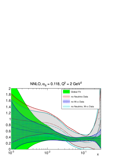
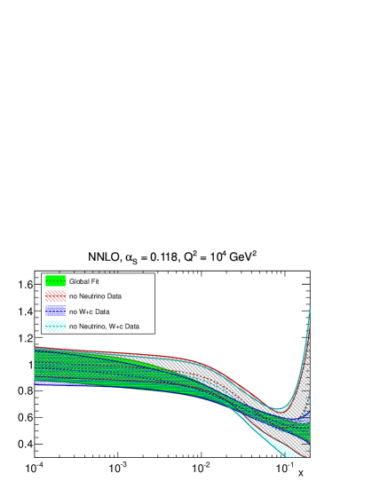
First, we observe the remarkable compatibility of the various fits (with, as usual, smaller uncertainty at a higher scale due to asymptotic freedom): for all fits and all the one-sigma PDF uncertainty bands overlap. The global fit is always the most accurate, though at very low and high scale the uncertainty is of similar size in all fits (in fact, it is even somewhat smaller in the fit without + than in the global fit, though this is a statistical fluctuation due to the large uncertainty on the uncertainty in this region). While when removing neutrino data the uncertainty blows up, removing the + has very little impact, leading to a moderate uncertainty reduction for when added to the fit without neutrino data. The fits without neutrino data do lead to a slightly higher central value of in the region of , but the effect is not significant on the scale of the uncertainty on these fits, though it would be significant on the scale of the uncertainty of the global fit. It must therefore be considered a statistical fluctuation due to the large uncertainty in the fit without neutrino data.
The for the relevant experiments in these various fits are collected in Tab. 15, thereby allowing us to compare how well each experiment is described when included or excluded from the fit. We see that + data are well described regardless of whether they are included in the fit or not, while the neutrino data are not well described unless they are included in the fit. This again shows that the impact of the + can only be moderate.
We conclude that the + data alone are not yet competitive with the neutrino data in determining strangeness, and that their inclusion does not modify significantly the assessment of the size of the nucleon strangeness in previous global fits, for which there is thus clear evidence for suppression in comparison to light quarks by a factor of between two and three at low scales.
| Global | No neutrino | No + | No neutrino/+ | |
|---|---|---|---|---|
| CHORUS | 1.13 | 3.87 | 1.09 | 3.45 |
| NuTeV | 0.62 | 4.31 | 0.66 | 6.45 |
| ATLAS 2010 | 1.21 | 1.05 | 1.24 | 1.08 |
| CMS + 2011 | 0.86 | 0.50 | 0.90 | 0.61 |
5.3 Stability
We will now check the dependence and stability of our results upon our methodology and its variations. Some of the issues which we address here were already studied in Sect. 4.5 in the context of closure tests, but others are specific to the fit to actual data.
Specifically, we will study the impact on the NNPDF3.0 results of the new minimization and stopping methodology discussed in Sect. 3.3 in comparison to that previously used in NNPDF2.3, the impact of the improved treatment of positivity discussed in Sect. 3.2.3, the impact of a multiplicative vs. additive treatment of systematic uncertainties (see Sect. 2.4.2), our improved self-consistent determination of preprocessing ranges presented in Sect. 3.2.2, and finally the independence of fitting basis (already tested in closure tests in Sect. 4.5.3).
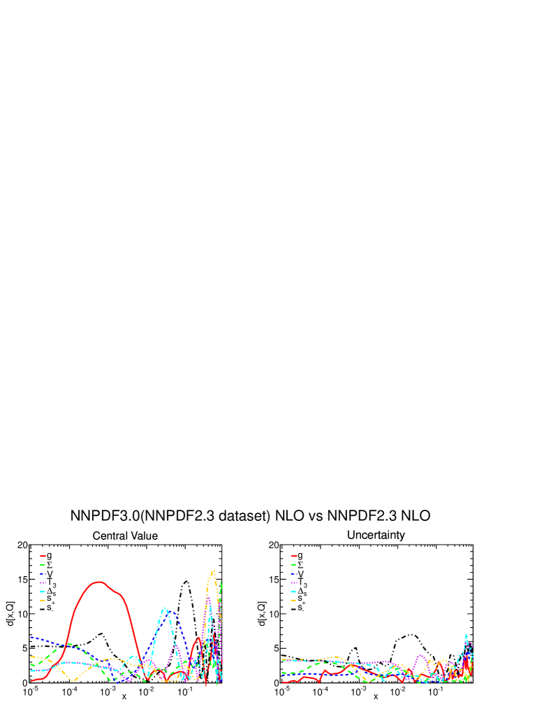
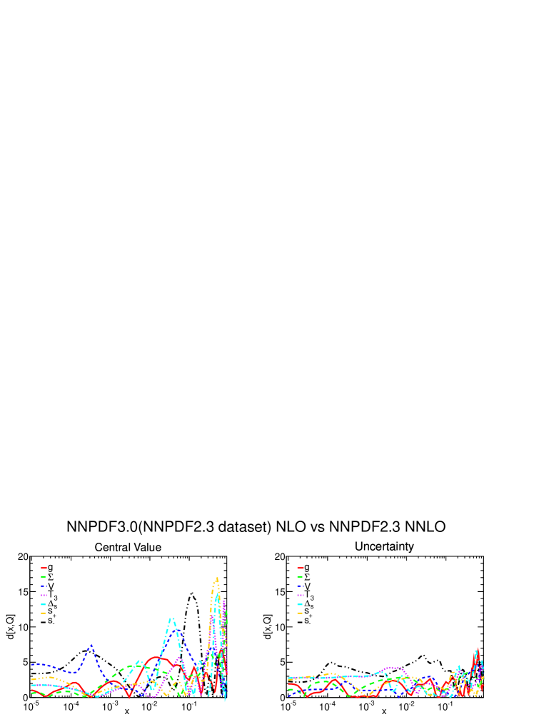
5.3.1 Impact of the NNPDF3.0 methodology
First, we discuss the impact of the NNPDF3.0 methodology, by comparing the NNPDF2.3 global fit with the fit discussed in Sect. 5.2.2 and shown in Fig. 46, based on an NNPDF2.3-like dataset, but with NNPDF3.0 methodology and theory settings (specifically the use of FONLL-B), i.e. by varying the methodology with fixed dataset. This is the complementary comparison to that which we performed in Sect. 5.2.2, where instead we varied the dataset with fixed methodology. With this comparison we can fully disentangle the effects of the new experimental data in NNPDF3.0 from that of the improved fitting methodology and the new theoretical settings.
The distances between the original NNPDF2.3 PDFs of Ref. [13] and the NNPDF3.0 fit with NNPDF2.3 data are shown in Fig. 55 both at NLO and NNLO, while the NNLO PDFs are compared in Fig. 56.
In the NLO fit the new methodology and theory settings have an impact on the small- gluon and large- quarks at the one and a half sigma level. The differences in the gluon can be understood as a consequence of having switched from the FONLL-A heavy quark scheme used in NNPDF2.3 to the more accurate FONLL-B adopted in NNPDF3.0, while the differences seen for quarks are necessarily a consequence of the more efficient methodology and extended positivity constraints (see Sect. 5.3.2 below). At NNLO the non-insignificant differences seen in all PDFs reflect the improved methodology and positivity, as the NNLO theory used in 2.3 and 3.0 is the same. At high scale the most noticeable difference is the softening of the small- gluon seen in Fig. 56.
The main conclusion of this comparison is that a significant part of the differences between the final NNPDF2.3 and NNPDF3.0 sets, as seen specifically at high scale in Fig. 31 and at low scale in Fig. 30, are due to the improved methodology (minimization and generalized positivity). This is consistent with the conclusion of Sect. 5.2.2 (see in particular Figs. 45-46) that the new data added in NNPDF3.0 have generally a moderate impact. In fact, we may cross-check the impact of the new methodology by comparing the of the fit to the NNPDF2.3-like dataset discussed in Sect. 5.2.2, to the of the original NNPDF2.3 fit to the same dataset: up to minor differences in the dataset, the difference in are then due to the methodology. With NNPDF2.3 PDFs we get , while with NNPDF3.0 methodology and an NNPDF2.3-like dataset we get , which is a small but non-negligible improvement, of more than 50 units in total , which must be entirely attributed to the new methodology.
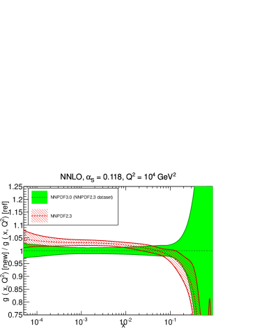
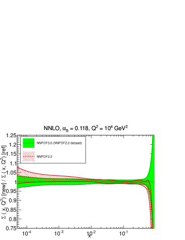
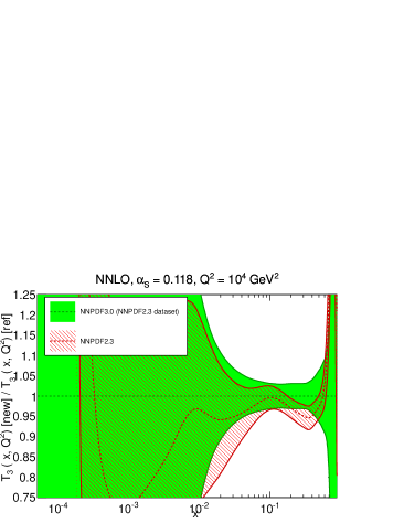
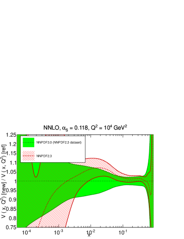
5.3.2 Constraints from positivity
As explained in Sect. 3.2.3, in NNPDF3.0 we adopt a more extensive set of positivity constraints: specifically now the number of constraints is equal to the number of PDFs (in fact, it exceeds them because the gluon is constrained by two different pseudo-observables), thereby ensuring not only positivity of the observables used in PDF fitting, but also of potential new observables such as cross-sections for new physics processes used in searches (see Sect. 5.4.4 below).
In order to quantify the impact of these positivity constraint, we have produced an unphysical variant of the NNPDF3.0 NNLO in which positivity constraints are removed (so in particular physical cross-sections could become negative). The distances between the default fit and the fit without positivity are shown in Fig. 57, while some of the PDFs which change most are compared in Fig. 58.
The impact of positivity is relatively mild except for the small- gluon and the large- strangeness, for which there is little direct experimental information. For all other PDFs and ranges the impact of positivity is below the one sigma level. Note that even so, strict positivity is necessary if one wishes to obtain meaningful predictions, e.g. in new physics searches. For the gluon, the effects of the positivity can be noticed already at , while at even smaller the gluon would become much more negative if positivity were not imposed: so the impact of positivity is to make the gluon less negative at small . For the strangeness asymmetry, interestingly, the dip-bump structure seen in the global fit is seen to be a consequence of positivity.
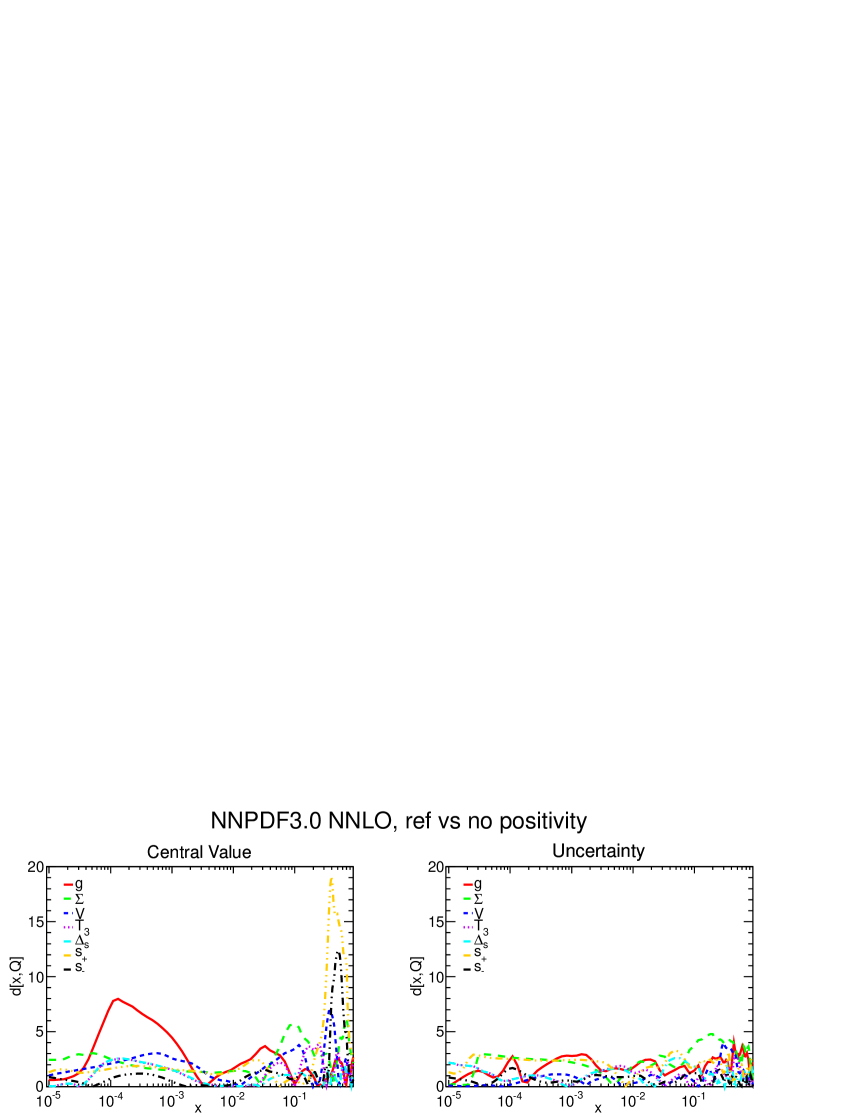
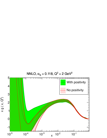

As a test of the efficiency of the Lagrange multiplier method we use to impose positivity, we have explicitly checked a posteriori that physical cross sections at NLO and NNLO are indeed not negative (note that because positivity is always imposed at NLO, as discussed in Sect. 3.2.3, small violations of positivity at NNLO are in principle possible). This is illustrated in Fig. 59, where we plot two pseudo-observables which are used to impose positivity, namely the light component of , and the Drell-Yan rapidity distribution: individual replicas are shown (green dashed curves) as well as the reference set in the positivity implementation (see Sect. 3.2.3), and the effectiveness of positivity (especially for the Drell-Yan distribution) is clearly seen.
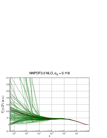
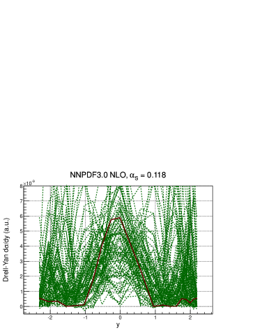
5.3.3 Additive versus multiplicative systematics
As discussed in Sect. 2.4.2, there is a certain latitude in the treatment of correlated systematics, in particular whether they are treated additively or multiplicatively (only normalization uncertainties being certainly multiplicative). In order to test the impact of the additive vs. multiplicative treatment of systematics, we have produced two modified version of the NNPDF3.0 fit, which only differ in the treatment of the systematics: in the first one we treat all systematics but the normalization as additive, and in the second, all systematics but the normalization is randomized, and treated as either additive or multiplicative at random for each replica. The default treatment (multiplicative or additive) of systematics is given in Tables 1 and 2 (fourth column).
The distances between these two fits and the default are shown in Fig. 60, while two PDFs for which the effect of the change is most noticeable are shown in Fig. 61 for the additive case, compared to the NNPDF3.0 default. The impact of the treatment of systematics turns out to be essentially indistinguishable from statistical fluctuations for all PDFs except the large- gluon, for which it can have an effect at the half-sigma level if all systematics is treated as additive. This can be understood as a consequence of the fact that the gluon depends strongly on jet data, which are affected by large systematics. The impact on the gluon is explicitly shown in Fig. 61. The singlet is also shown: in this case, the change in uncertainty at small seen in the plot is actually compatible with a statistical fluctuations, as the distance plot Fig. 60 demonstrates. When systematics are randomized the effect is diluted and the changes are always compatible with statistical fluctuations.
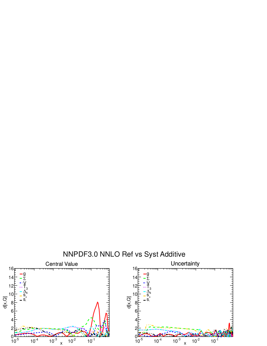
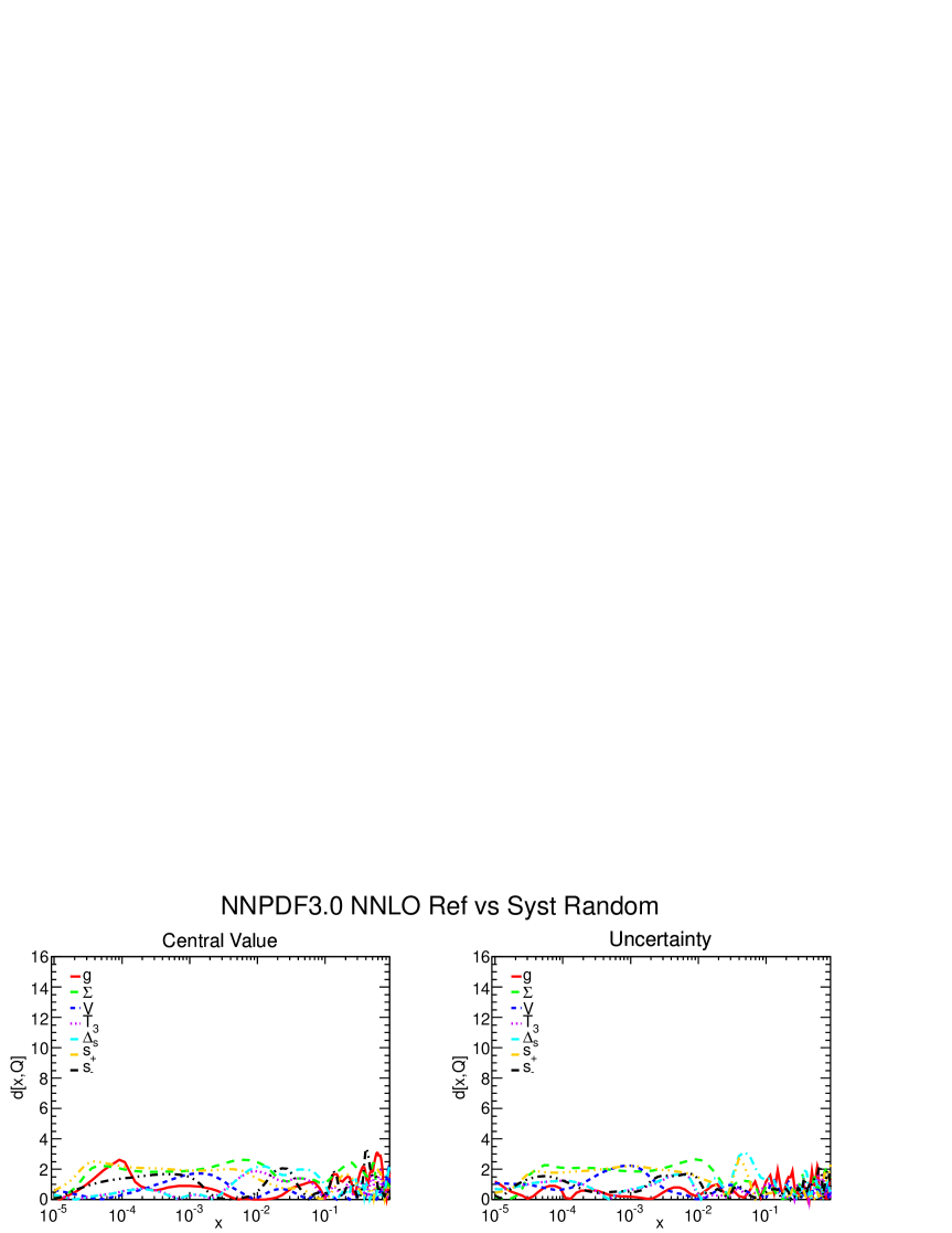
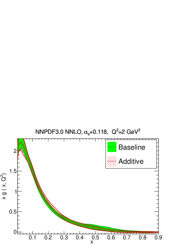
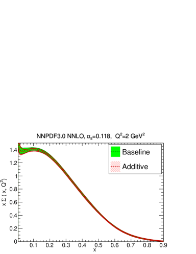
We conclude that the treatment of systematics, while an issue in principle, in practice affects results at a level which is compatible with fluctuations: in the absence of information on how to treat the systematics this would be randomized, but then results are compatible with the default. Even when all systematics are treated as additive, which is an extreme case, only the gluon changes significantly: but then the gluon is mostly affected by HERA and jet data, for both of which the preferred treatment of systematics is multiplicative [172, 173]. The default treatment of systematics in the NNPDF3.0 fit thus appears to be both reliable and robust.
5.3.4 Independence of preprocessing
As discussed in Sect. 3.2.2, in NNPDF3.0 the preprocessing exponents which characterize the function that relates PDFs to their neural network parametrization according to Eq. (9) are determined self-consistently. This method has been already used in NNPDF polarized PDF fits [143, 144]. We now check that indeed the method works, and specifically that the ranges of the effective exponents Eq. (11-12) are well within the preprocessing ranges, and thus not biased by it.
The effective exponents and preprocessing ranges for the gluon and singlet in the global NNPDF3.0 NLO fit are shown in Fig. 62: the green solid band is the 68% confidence level interval for each effective exponent as a function of , for the replica fit, and the green dashed line is twice this interval. The red hatched band (and the red dashed lines) are the corresponding results obtained from the replica fit. In each case, the black solid horizontal lines are the extremes of the preprocessing range, determined from the effective exponents of a previous fit according to the procedure discussed in Sect. 3.2.2. The preprocessing range is self-consistent in the sense that if the range is determined again from the values of the effective exponents shown in Fig. 62 it is essentially unchanged, as it can be seen from visual inspection of the plot.
It is furthermore clear that indeed the effective range is always well within the allowed preprocessing range, thereby ensuring that the former is not influenced or distorted by the latter. We have checked that this is the case for all PDFs and all PDF sets discussed in this paper. Of course, when changing substantially the dataset, such as, for example, when constructing the HERA-only PDFs of Sect. 5.2, the preprocessing ranges may change significantly (with fewer data the acceptable ranges are generally wider) and thus the procedure has to be iterated again for convergence.

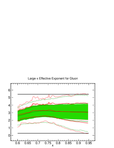

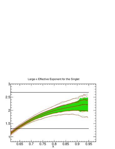
5.3.5 Independence of the PDF fitting basis
We finally wish to test for independence of the fit results of the choice of PDF basis. This was already tested explicitly in Sect. 4 in the framework of a closure test, and it is now verified for the fit to actual data, which is possibly more complicated, both because the final NNPDF3.0 PDFs have sometimes more structure than the MSTW2008 PDFs used in that closure test, and also because of potential inconsistencies between data which are by construction absent in a closure test. It is worth pointing out that this independence is usually not achieved, or at least not completely, by PDF determinations based on a standard functional forms, as shown in Ref. [174].
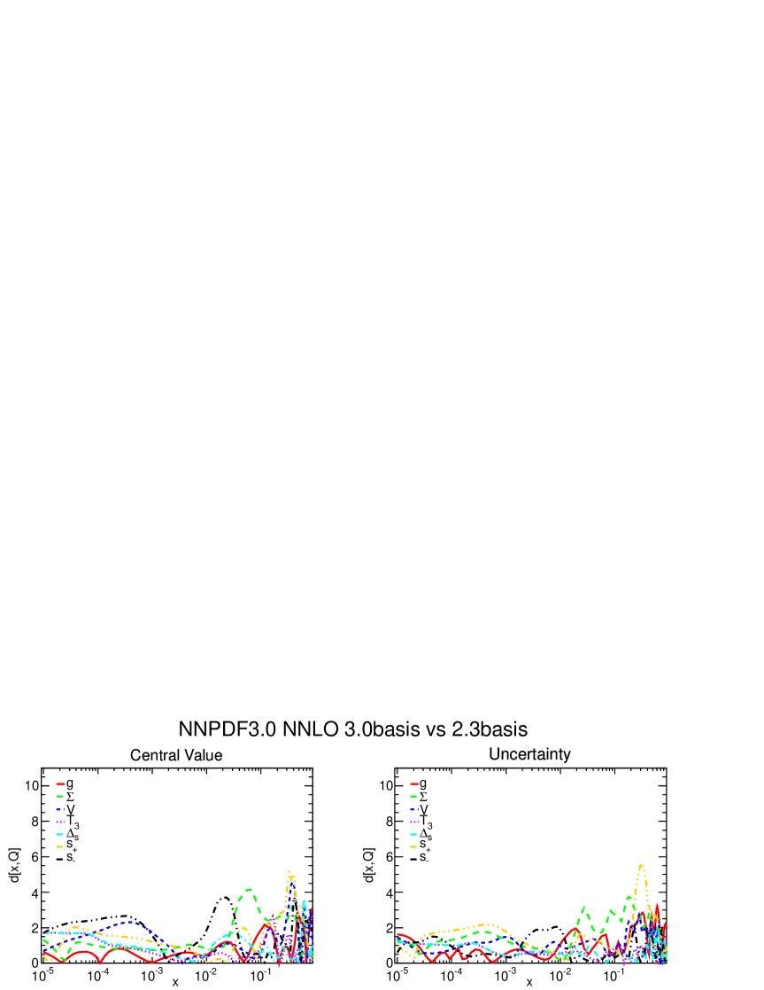
In Fig. 63 we show the distances between the default NNPDF3.0 NNLO PDFs and the same fit but using the NNPDF2.3 fitting PDF basis Eq. (7) instead of the default NNPDF3.0 basis Eq. (8) for the parametrization of input PDFs. Results are consistent to what was found in the closure test: distances are mostly compatible with statistical equivalence, with only strangeness (whose parametrization is affected by the change of basis) deviating at the half-sigma level at the valence peak, which is above the threshold of statistical indistinguishability. Note that the dip-bump structure in seen in Fig. 58 (and related to positivity) arises due to interference of different PDFs in the NNPDF2.3 basis, yet it is perfectly reproduced, thereby confirming the remarkable stability of the NNPDF3.0 results.
5.4 Implications for LHC phenomenology
We now turn to a brief preliminary investigation of the implications of NNPDF3.0 PDFs for LHC phenomenology. We start by comparing the NNLO PDF luminosities at 13 TeV, both to NNPDF2.3, with CT10 and MMHT. Then we move to predictions for a variety of LHC cross-sections at 13 TeV, which we compute at NLO using the automated MadGraph5_aMC@NLO program [114], and for which we compare results obtained using NNPDF2.3 and NNPDF3.0 PDFs: specifically, vector boson, top, and Higgs production. Then we turn to the implications of NNPDF3.0 PDFs for the dominant Higgs production channel at the LHC, gluon-fusion, and provide NNLO cross-sections computed with the iHixs code [155], including a study the dependence of results on the dataset used for PDF determination. Finally, we study the production of high-mass states, close to the LHC kinematic threshold, as relevant for searches of massive New Physics at the energy frontier.
5.4.1 PDF luminosities
In Fig. 64 we compare the PDF luminosities obtained using the NNPDF3.0 set and discussed in Sect. 5.1.2 to CT10 [150, 151] and MMHT14 [162]. Note that these comparisons might become obsolete once CT10 PDFs are updated, though they will be easily updated using the recent APFEL tool [175]. The three sets are consistent within their uncertainties. Quite in general NNPDF3.0 has smaller uncertainties in the data region, but larger uncertainties in the extrapolation regions. For the luminosity in the region relevant for Higgs production, the agreement between the three sets has improved in comparison to previous benchmarks using NNPDF2.3 and MSTW2008 [139]. Large differences in central values are found for large values of , relevant for the production of very massive New Physics particles, though all sets are compatible within their very large uncertainties.
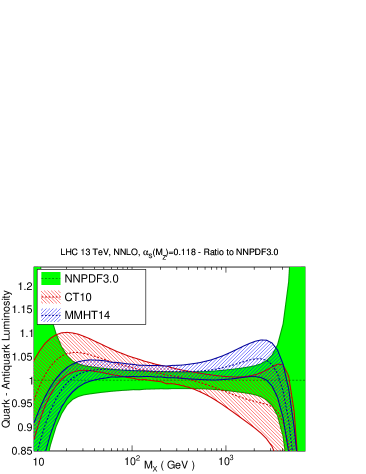
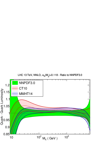
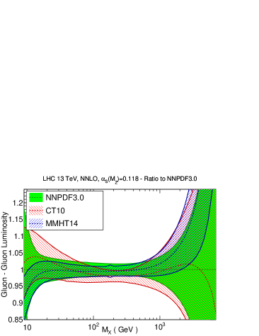
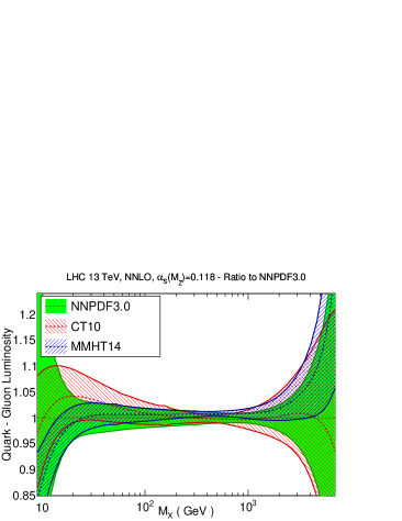
5.4.2 Implications for =13 TeV LHC processes
An extensive phenomenological comparison of NNPDF3.0 for all processes and a wide range of PDF sets is beyond the scope of this work. We will thus only compare NNPDF2.3 and NNPDF3.0, for a limited set of LHC observables. Unless otherwise stated, we use the NLO sets with and work in the variable-flavor-number scheme with massless bottom quarks. Theoretical predictions at NLO are computed using the MadGraph5_aMC@NLO program [114], version 2.1.2, interfaced to LHAPDF6. The NLO results are sufficient to assess the PDF dependence of these observables, as typically the NNLO/NLO –factor have a weak PDF dependence. In addition to NNPDF3.0 global fit results, we also provide predictions using the conservative parton set with as an illustration of results found using a maximally consistent dataset (see [176]).
Even though we do not aim to a direct comparison to the raw data, cross-sections have been computed at the fiducial level, including resonance decays for some processes, and using realistic generation cuts. Jets are reconstructed with the anti- algorithm [177] with radius , and the following cuts are applied to all jets in the final state:
| (37) |
For final-state leptons, the following cuts are applied:
| (38) |
Finally, for photons we impose
| (39) |
and use the Frixione isolation criterion [178], with and and an isolation cone radius . No further analysis cuts are applied. Renormalization and factorization scales are set dynamically event by event to , with the scalar sum of the transverse energies of all the final-state particles. Within each run, PDF and scale uncertainties in MadGraph5_aMC@NLO are obtained at no extra cost using the reweighting technique introduced in Ref. [179]: we thus provide in each case both the central value and the PDF uncertainty.
| Process | NNPDF2.3 | NNPDF3.0 | RelDiff | NNPDF3.0 |
| 1.403 nb ( 1.5%) | 1.404 nb ( 2.0%) | +0.1% | 1.45 nb ( 2.0%) | |
| 10.30 nb ( 1.3%) | 10.21 nb ( 1.9%) | -0.9% | 10.29 nb ( 2.3%) | |
| 7.67 nb ( 1.3%) | 7.75 nb ( 1.9%) | +1.1% | 7.96 nb ( 1.9%) | |
| 2.665 nb ( 3.5%) | 2.680 nb ( 4.2%) | +0.56% | 2.807 nb ( 8.8%) | |
| 2.353 nb ( 1.2%) | 2.332 nb ( 1.5%) | -0.9% | 2.325 nb ( 1.6%) | |
| 62.24 nb ( 1.2%) | 63.85 ( 1.8%) | +2.6% | 61.51 ( 1.9%) | |
| 678 pb ( 1.7%) | 672 pb ( 1.6%) | -0.9% | 655 pb ( 3.3%) | |
| 26.48 fb ( 1.4%) | 26.58 fb ( 1.5%) | +0.4% | 27.07 fb ( 2.3%) | |
| 0.134 pb ( 1.6%) | 0.131 pb ( 1.6%) | -2.2% | 0.137 pb ( 2.6%) | |
| 0.458 pb ( 2.2%) | 0.4595 pb ( 1.7%) | +0.6% | 0.459 pb ( 4.0%) |
Results are collected in Tab. 16, where processes are grouped into three subsets: processes which are sensitive to quark and antiquarks, processes which are sensitive to the gluon PDF, and Higgs production processes, except gluon fusion which is discussed in the next section. The results of Tab. 16 are also represented in Fig. 65, normalized to NNPDF2.3.
For all these cross-section a remarkable stability between NNPDF2.3 and NNPDF3.0 is observed, with all results varying by no more that the size of the corresponding PDF uncertainty. For top-quark pair production, going from NNPDF2.3 to NNPDF3.0 the cross-section increases by about 1%, about half the PDF uncertainty. This can be understood recalling that thee NNPDF3.0 luminosity is harder than is NNPDF2.3 counterpart for GeV; this also explains the behaviour of the closely related production process. Note that NNPDF2.3 already gave a very good description of all available ATLAS and CMS 7 TeV and 8 TeV production data [76], even though they were not included in the fit. For production in association with charm quarks, we use a scheme in order to retain the full charm mass dependence. For this observable, results are very stable when moving from NNPDF2.3 to NNPDF3.0.
Coming now to Higgs production, for the NNPDF3.0 result is about 2.3% larger than the NNPDF2.3 prediction, consistent with the expectation from the luminosity comparisons in Fig. 32 for GeV (recall that the calculation uses a dynamical setting of the factorization scale). For the associate production channels, and , driven by the luminosities, differences are well within one sigma, as expected from the luminosities of Fig. 32.
Coming finally to the comparison with the conservative PDFs, we note that prediction obtained using the latter are generally consistent at the one sigma level with the default ones, occasionally with differences at the two sigma level, such as for example for .
Of course, predictions from conservative partons are generally affected by larger PDF uncertainties because of the smaller dataset, though in some cases they are only slightly less accurate than the global fit, such as for example for inclusive and production. On the other hand, for processes that depend on strangeness (like +) or that are gluon-driven (like and ) the PDF uncertainties are substantially larger in the conservative partons than in the global fit.
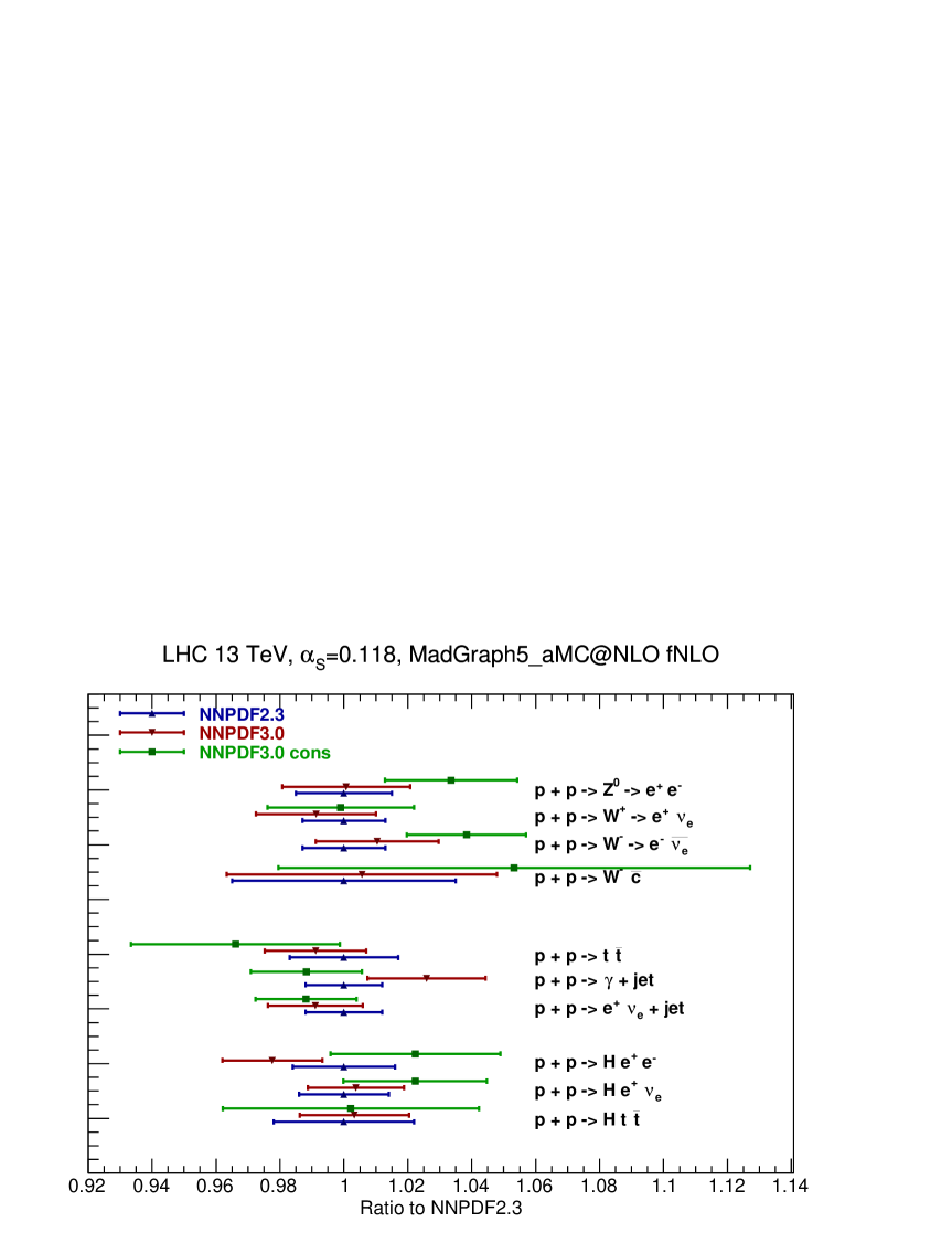
5.4.3 Higgs production in gluon fusion
We now focus specifically on Higgs production in gluon fusion, the dominant channel at the LHC, for which theoretical uncertainties are a limiting factor for the determination of Higgs properties. We provide predictions for the total cross-section at NLO and NNLO for the LHC 13 TeV, comparing the default NNPDF3.0 set to NNPDF2.3 and to the various sets based on alternative datasets discussed in Sect. 5.2, with the main goal of studying the dependence of this prediction on the underlying PDFs, along the lines of the study presented in Ref. [168]. The uncertainties shown are pure PDF uncertainties, with , i.e. the uncertainty is not included. The inclusive cross-section is computed using iHixs 1.3.3, with GeV, renormalization and factorization scales set to and the infinite top mass (effective theory) approach. Clearly, our predictions are not meant to be realistic, however, the effects which we do not include (such as for instance electroweak corrections, or finite top, bottom and charm mass contributions) have a negligible PDF dependence, while uncertainties are completely independent of the PDF uncertainty, given that the PDF and uncertainties combine in quadrature in the gaussian case even when correlated [180]. Hence our results do provide an accurate assessment of the PDF dependence of the cross-section and its uncertainty.
Results are collected in Tab. 17, and summarized graphically in Figs. 66-67. We show results obtained using NNPDF2.3, and the following NNPDF3.0 sets: 2.3-like dataset, default, conservative with , no jet data, no LHC data and HERA-only, all of which have been discussed in detail in Sect. 5.2. In Tab. 17 we also show the pull of each prediction compared to the NNPDF2.3 result, defined as
| (40) |
where is the one-sigma PDF uncertainty.
As expected from the comparison of the gluon-gluon luminosities in Fig. 33, the NNLO cross-section decreases by about 2-sigma when going from NNPDF2.3 to NNPDF3.0, while the PDF uncertainty increases substantially. At NLO the effect is less marked, with the NNPDF2.3 and NNPDF3.0 in agreement at the one-sigma level. Because a similar result is found using NNPDF3.0 PDFs based on a 2.3-like dataset we must conclude that the change is mostly due to methodological improvements, rather than the underlying data. Because of the validation from closure testing, the NNPDF3.0 results are more reliable, both in terms of central values and uncertainties.
| (pb) NLO | Pull | (pb) NNLO | Pull | |
|---|---|---|---|---|
| NNPDF2.3 | 34.72 0.33 | - | 46.39 0.46 | - |
| NNPDF3.0 with 2.3 data | 34.06 0.57 | 1.0 | 45.14 0.74 | 1.4 |
| NNPDF3.0 global | 33.96 0.61 | 1.1 | 45.01 0.72 | 1.6 |
| NNPDF3.0 conservative | 33.31 0.54 | 2.2 | 43.70 1.12 | 2.2 |
| NNPDF3.0 no Jets | 34.56 1.04 | 0.2 | 45.32 0.92 | 1.0 |
| NNPDF3.0 noLHC | 34.12 0.80 | 0.7 | 45.10 0.91 | 1.3 |
| NNPDF3.0 HERA-only | 31.96 3.03 | 0.9 | 43.02 2.21 | 1.5 |
Results obtained using NNPDF3.0 sets based on alternative datasets are always mutually consistent at the one sigma level, with the conservative partons leading to a lower result and the fit with no jets to a slightly higher one but with significantly larger uncertainty. The lowest central value is found using the HERA-only set, which however is affected by a PDF uncertainty which is by a factor three larger than the default.
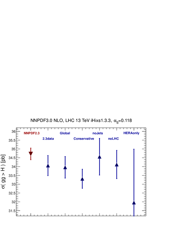
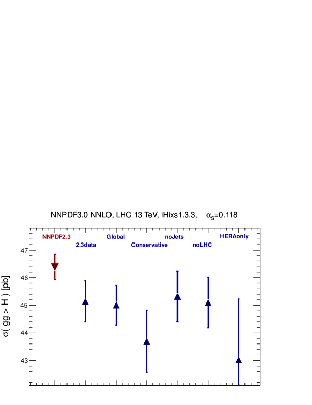
Despite these variations in results, all pulls are of similar size, between 0.7 and 1.1 at NLO and between 1.3 and 1.6 at NNLO, with the only exception of conservative partons, which have a larger pull of 2.2 both at NLO and NNLO. This means that the dependence of the results on the dataset appears to be consistent with statistical fluctuations.
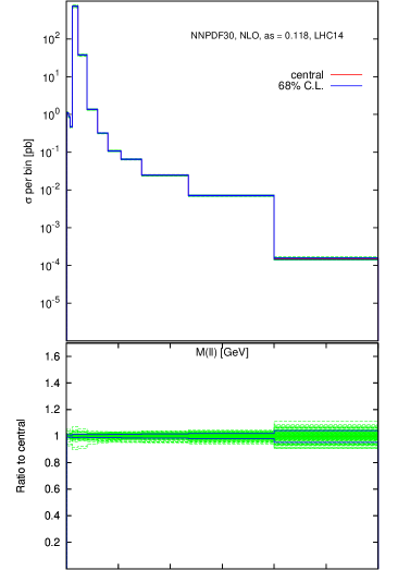
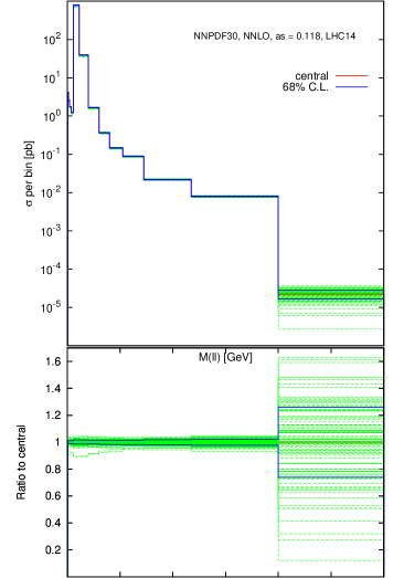
5.4.4 New Physics particle production at high masses
A wide variety of scenarios of physics beyond the standard model include heavy particles at the TeV scale that could be within the reach of the LHC. Production of very massive particles probes PDFs at large , where they are poorly known due to the lack of direct experimental information, and thus the corresponding predictions are affected by substantial PDF uncertainties (see e.g. Refs. [181, 182]). Consequently, PDFs can be a limiting factor in the determination of exclusion regions, and improving their knowledge can lead to an increase in the search potential. In this context an accurate assessment of their uncertainties is therefore crucial. The unbiased NNPDF approach is advantageous in this respect in that it leads to uncertainty estimates which are not biased by assumptions on the functional form of PDFs. The only significant constraint on PDFs close to threshold comes from positivity, which is now implemented in an optimal way as we discussed in Sects. 3.2.3-5.3.2 above.
As an example, we consider high-mass Drell-Yan production and the pair production of supersymmetric particles. High-mass dilepton production is frequently used to search for new physics that couples to the electroweak sector, and thus it is important to provide precise predictions for the SM production mechanisms.
We have computed the dilepton invariant mass distribution in events at the LHC 14 TeV with NNPDF3.0 at NLO and NNLO using FEWZ. Recall from Sect. 3.2.3 that positivity is always imposed at NLO, so an explicit check of positivity of the NNLO result is nontrivial. Results are shown in Fig. 68, in different bins: each of the NLO (left) or NNLO (right) Monte Carlo replicas is shown as a green dashed line, together with the corresponding central values and one-sigma intervals. All MC replicas are positive up to the highest invariant mass bins.
As a second example, we provide predictions for the pair production of supersymmetric particles at the LHC 14 TeV. The computation has been performed using Prospino [183, 184] with NNPDF3.0 NLO, using settings as close as possible to those of Refs. [181, 182], though the only relevant physical input for our illustrative study are the sparticle masses. Note that for this processes NNLO calculations are not available. We have produced results for squark-squark, squark-antisquark and gluino-gluino production, for three different values of the sparticle masses, namely 1 TeV, 2 TeV and 3 TeV. We show the predictions for the Monte Carlo replicas of NNPDF3.0 for the squark-antisquark and gluino-gluino channels; the squark-squark cross-section (not shown) is always positive in the mass range that we are considering. In each case, we also provide the average result and the 68% confidence level interval. For comparison, predictions using the NNPDF2.3 NLO PDFs are also shown.
Results are shown in Fig. 69. In the case of gluino-gluino production (right), all replicas are strictly positive up to TeV. At 3 TeV, some replicas lead to slightly negative cross-sections: 15 in NNPDF2.3, and only 3 in NNPDF3.0. In both cases, the 68% confidence levels are always positive; we conclude that the occasional negative replica can be set to zero with no impact on the central value or uncertainty. For squark-antisquark production (left) all cross sections are positive up to TeV, while for TeV some cross-sections are slightly negative. For NNPDF2.3, the central value was negative, while now for NNPDF3.0 the central value is positive and only a small part of the 68% confidence level range is in the negative region. This means that our improved positivity is still not fully efficient, and it allows some replicas to lead to negative cross-section: partly because positivity is imposed with a Lagrange multiplier which carries a large but finite penalty, and also, because positivity is only imposed for standard model processes, and not for all possible processes. Setting these negative cross-sections to zero would of course not modify the upper uncertainty range, implying that for this particular subprocesses and sparticle masses arbitrarily small production cross-sections are allowed within the large PDF uncertainties. Note however the very large PDF uncertainties at the largest masses: for example, for squark-antisquark production, the 68% CL range for the cross-section for 3 TeV is pb, with a central value of pb.
We conclude that, thanks to the improved implementation of positivity in NNPDF3.0, the cross-section for high-mass particle production is positive, thereby improving over NNPDF2.3. Occasional replicas leading to negative cross-sections very close to threshold can be set to zero without significantly affecting central values and uncertainties.
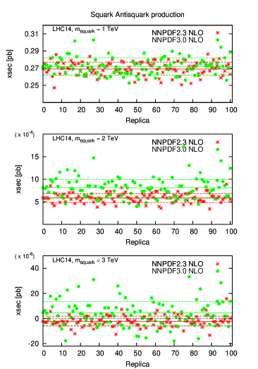

6 Summary and outlook
We conclude by summarizing the NNPDF3.0 fits that will be made public, their use in specific phenomenological application, and future developments.
All PDF sets are made available via the LHAPDF6 library [185], from version 6.1.4 onward,
For the global fits, we also provide the corresponding grids in LHAPDF5 format via the the NNPDF HepForge webpage,
though whenever possible, the modern v6 interface should be used.
The interpolation used in the delivery of NNPDF sets has been substantially improved in the transition from LHAPDF5 to LHAPDF6.
-
•
The default interpolation algorithms, of LHAPDF6 are now used, instead of the in-house interpolation used by NNPDF sets in LHAPDF5. These algorithms are faster and more accurate, but we have checked that in most of the relevant range of and the LHAPDF6 and LHAPDF5 algorithms agree at the permille level.
-
•
A wider range for the and grids is now adopted: the NNPDF3.0 sets can be used for
(41) which is adequate for future phenomenological applications, including calculations of cross-section of ultra-high energy neutrinos, which require PDFs down to , and studies of a Future Circular Collider with a center-of-mass energy of 100 TeV. Outside the range in Eq. (41), where no experimental information is available, the values of the PDFs are frozen.
-
•
Thanks to the novel functionalities in LHAPDF6, for all the NNPDF3.0 sets the interpolation grid has been divided into different subgrids separated by heavy quark thresholds. This ensures that the correct threshold behavior of the heavy quark PDFs is satisfied also by the interpolation, and in particular that the heavy quark PDFs are exactly zero below the threshold.
The NNPDF3.0 PDF sets to be made available via LHAPDF6 are the following:
-
•
Global NNPDF3.0 sets - baseline fits
The baseline LO, NLO and NNLO NNPDF3.0 sets are based on the global dataset, with and a variable-flavor number with up to five active flavors, the convention for the corresponding LHAPDF6 grid files is
NNPDF30_lo_as_0118
NNPDF30_nlo_as_0118
NNPDF30_nnlo_as_0118The leading order NNPDF3.0 allows, among other applications, to compare theoretical predictions for cross-sections computed at different perturbative orders. In LHAPDF6, the output of the NNPDF3.0 LO PDFs is forced to be positive using the suitable meta-data instructions. For uses in leading-order Monte Carlo event generators, we still recommend the use NNPDF2.3LO, since, as part of the updated Monash 2013 Tune [156] of Pythia8 [186], it has been shown to provide an excellent description of a variety of soft and semi-hard data.
-
•
Global NNPDF3.0 sets - fits with variations
Using the same global dataset as above, for the NLO and NNLO fits we have produced fits with different values of , that can be used to evaluate the combined PDF+ uncertainties in cross-sections:
NNPDF30_nlo_as_0115, NNPDF30_nlo_as_0117, NNPDF30_nlo_as_0119, NNPDF30_nlo_as_0121
NNPDF30_nnlo_as_0115, NNPDF30_nnlo_as_0117, NNPDF30_nnlo_as_0119, NNPDF30_nnlo_as_0121The procedure to combine PDF and uncertainties in a Monte Carlo set like NNPDF3.0 is explained in [135] (see also Ref. [187]). The choice of the uncertainty to be assigned to the strong coupling is left to the PDF users. For LO, we also provide a fit with , as this is the value typically required in LO calculations:
NNPDF30_lo_as_0130
Note that from the NLO and NNLO range of values, the predictions for any other value of not included in the list can be easily obtained from either interpolation or extrapolation.
-
•
Global NNPDF3.0 - fits with different maximum number of active flavors
For various important phenomenological applications, PDF sets in which either the charm quark or both the charm and bottom quarks are treated as massive are required. In the following we denote these two schemes as the and schemes. In order to obtain and versions of the NNPDF3.0 sets, we follow the procedure outlined in [11]. We start from the baseline NNPDF3.0 fits, where the charm and bottom quarks are massless parton ( scheme), at the input scale, GeV2. This boundary condition is then evolved upwards in , but using the and schemes, to produce the desired sets with different maximum number of active partons. This has been done for a reduced range of values, to be able to compute the combined PDF+ uncertainties. These fits are:
NNPDF30_nlo_as_0117_nf3, NNPDF30_nlo_as_0118_nf3, NNPDF30_nlo_as_0119_nf3
NNPDF30_nnlo_as_0117_nf3, NNPDF30_nnlo_as_0118_nf3, NNPDF30_nnlo_as_0119_nf3
NNPDF30_nlo_as_0117_nf4, NNPDF30_nlo_as_0118_nf4, NNPDF30_nlo_as_0119_nf4
NNPDF30_nnlo_as_0117_nf4, NNPDF30_nnlo_as_0118_nf4, NNPDF30_nnlo_as_0119_nf4In addition, using a similar procedure we have provided sets in the scheme, that is, treating the top quark as a massless parton. While treating the top quark as massless is not justified at the LHC, it might become appropriate at higher energy colliders, see for example Ref. [188]. These sets that include the top PDF are denoted as
NNPDF30_nlo_as_0117_nf6, NNPDF30_nlo_as_0118_nf6, NNPDF30_nlo_as_0119_nf6
NNPDF30_nnlo_as_0117_nf6, NNPDF30_nnlo_as_0118_nf6, NNPDF30_nnlo_as_0119_nf6Likewise, we also provide similar fits with different maximum number of active flavors for the LO fits, for the two values of used:
NNPDF30_lo_as_0118_nf3, NNPDF30_lo_as_0118_nf4, NNPDF30_lo_as_0118_nf6,
NNPDF30_lo_as_0130_nf3, NNPDF30_lo_as_0130_nf4, NNPDF30_lo_as_0130_nf6 -
•
Fits based on reduced datasets
We have also released fits based on reduced datasets, as discussed in detail in Sect. 5.2. First, conservative partons, for which the fit with the choice of threshold value of is used. We provide results in the restricted range of values:
NNPDF30_nlo_as_0117_cons, NNPDF30_nlo_as_0118_cons, NNPDF30_nlo_as_0119_cons
NNPDF30_nnlo_as_0117_cons, NNPDF30_nnlo_as_0118_cons, NNPDF30_nnlo_as_0119_consThen, HERA-only PDFs, which may be useful to gauge the impact of new LHC measurements:
NNPDF30_nlo_as_0117_hera, NNPDF30_nlo_as_0118_hera, NNPDF30_nlo_as_0119_hera
NNPDF30_nnlo_as_0117_hera, NNPDF30_nnlo_as_0118_hera, NNPDF30_nnlo_as_0119_heraIn view of possible reweighting applications, for the central value of also sets are provided,
NNPDF30_nlo_as_0118_hera_1000
NNPDF30_nnlo_as_0118_hera_1000Next, HERA+ATLAS and HERA+CMS fits. These can be useful to compare with analogous fits presented by the LHC collaborations, and are labeled as
NNPDF30_nlo_as_0117_atlas, NNPDF30_nlo_as_0118_atlas, NNPDF30_nlo_as_0119_atlas
NNPDF30_nnlo_as_0117_atlas, NNPDF30_nnlo_as_0118_atlas, NNPDF30_nnlo_as_0119_atlas
NNPDF30_nlo_as_0117_cms, NNPDF30_nlo_as_0118_cms, NNPDF30_nlo_as_0119_cms
NNPDF30_nnlo_as_0117_cms, NNPDF30_nnlo_as_0118_cms, NNPDF30_nnlo_as_0119_cmsThen, sets without LHC data, sometimes used for theory comparisons with LHC measurements. Also here, in view of possible reweighting exercises with LHC data, we provide for the central value of a set of replicas:
NNPDF30_nlo_as_0117_nolhc, NNPDF30_nlo_as_0118_nolhc, NNPDF30_nlo_as_0119_nolhc
NNPDF30_nlo_as_0118_nolhc_1000
NNPDF30_nnlo_as_0117_nolhc, NNPDF30_nnlo_as_0118_nolhc, NNPDF30_nnlo_as_0119_nolhc
NNPDF30_nnlo_as_0118_nolhc_1000Finally, a fit excluding all jet data, which avoids the use of approximate NNLO results. Again, these are provided in a range of values, and denoted by
NNPDF30_nlo_as_0117_nojet, NNPDF30_nlo_as_0118_nojet, NNPDF30_nlo_as_0119_nojet
NNPDF30_nnlo_as_0117_nojet, NNPDF30_nnlo_as_0118_nojet, NNPDF30_nnlo_as_0119_nojet
Note that for all fits for which replicas are available, the corresponding replica sets have been obtained using independent random seeds, so that the and replica sets are fully independent.
Now that PDFs validated by a closure test, and fitted to a wide variety of LHC data are available, three main directions of progress are foreseen. From a methodological point of view, some optimization is still possible: specifically by producing sets with a reduced number of PDF replicas which retain as much as possible of the information from the full dataset. From the phenomenological point of view, new data will be added to the dataset as soon as they become available. These include the final combined HERA dataset, jet data from ATLAS and CMS from the 2011 and 2012 runs, and electroweak gauge boson production at 8 TeV, and, in the longer term, LHC data from Run II will also be included. Finally, from the theory point of view we plan to improve the treatment of heavy quarks by introducing an intrinsic charm PDFs, to provide PDF sets based on resummed QCD theory, and to produce QCD+QED sets including a full fit of the photon PDF.
With data, methodology and theory under control the main outstanding issue is a full characterization of theoretical uncertainties on PDFs, which remains an open problem. It will have to be addressed in order for parton distributions to become a controlled tool for precision physics at present and future colliders.
Acknowledgments
We thank L. Lyons for stressing the importance of closure testing of
parton distributions, and A. de Roeck, A. David, J. Huston,
M. Mangano, A. Mitov, P. Nadolsky,
G. Passarino, G. Salam, R. Tanaka,
R. Thorne and G. Watt for many illuminating discussions.
We thank F. Petriello for his help in running FEWZ
and comparing the results and G. Ferrera
for his help in setting up DYNNLO.
We are grateful to S. Glazov for support with the HERA-II H1 data;
A. Cooper-Sarkar and I. Abt for support with the ZEUS
HERA-II data; S. Glazov, C. Gwenlan and A. Tricoli
for information about the
ATLAS measurements; J. Alcaraz,
J. Berryhill, M. Cepeda, M. Gouzevitch, I. Josa, K. Lipka and K. Rabbertz for
assistance with the CMS data; and D. Ward,
J. Anderson, K. Mueller, R. McNulty
and T. Shears for help with the LHCb electroweak measurements.
V. B. is supported by the ERC grant 291377, “LHCtheory: Theoretical predictions and analyses of LHC physics: advancing the precision frontier”. S. F. and S. C. are supported in part by an Italian PRIN2010 grant, by a European Investment Bank EIBURS grant, and by the European Commission through the HiggsTools Initial Training Network PITN-GA-2012-316704. J. R. is supported by an STFC Rutherford Fellowship ST/K005227/1. J. R. and N. H. are supported by an European Research Council Starting Grant ”PDF4BSM”. R. D. B. and L. D. D. are funded by an STFC Consolidated Grant ST/J000329/1.
Appendix A QCD and weak corrections to vector boson production data
In this appendix we provide a detailed overview of the theoretical calculations that we have used to include LHC vector boson production data in the NNPDF3.0 analysis. For each datapoint, we provide the size of the NNLO QCD and of the NLO weak corrections, comparing with the total experimental uncertainty. Results for the QCD and weak corrections are given for all the LHC neutral current Drell-Yan measurements included in NNPDF3.0, namely for the CMS double differential distributions from the 2011 run [59], the ATLAS high mass Drell-Yan distributions from the 2011 run [56], the ATLAS boson rapidity distribution from the 2010 run [47], and for LHCb rapidity distributions in the forward region from the 2011 run [61]. Using these calculations, here we also provide, for the neutral-current Drell-Yan data, the NNLO and weak -factors, defined as in Sect. 2.3.
As we will show now, the effect of the pure weak corrections is negligible for neutral-current Drell-Yan data around peak region, and it becomes numerically important for small and large values of the dilepton mass . For charged-current Drell-Yan production, weak corrections are small outside the peak region (where all the available data lies) and thus can be safely neglected in the present analysis. For charged-current DY, NNLO QCD corrections are moderate; they have been included in the NNPDF3.0 analysis but are not discussed explicitly in this Appendix.
In this work, theoretical predictions are obtained with FEWZ3.1 [120] and have been cross-checked against DYNNLO1.3 [115]. The NNPDF2.3 NLO set with is used as input for the NLO theoretical predictions, and NNPDF2.3 NNLO is used for the corresponding NNLO calculations, as well as to determine the –factors. The scheme is adopted for all electroweak computations, where the input parameters are , and , while and may be obtained from these using:
| (42) |
where . In this analysis we use GeV-2 , GeV, GeV and do not adopt the narrow-width approximation.
A.1 CMS double differential distributions
The CMS experiment has measured [59] the lepton pair rapidity distributions for the Drell-Yan process in six bins of the invariant mass of the final state lepton pair, . For each bin in , the distribution is divided in 24 equally spaced bins in rapidity, up to , except for the last bin in that is divided in 12 bins. In the theoretical calculations, we set and to the average value of each dilepton invariant mass bin. The cuts on the final state leptons are the following:
with () being the transverse momentum of the softer (harder) lepton, and are the rapidities of the two leptons. In Tabs. 18-23 we provide the results of our calculations, and compare the total experimental uncertainty with the corresponding NNLO QCD and the NLO pure weak corrections, for the six bins in invariant mass of this measurement.
The NNLO corrections to this measurement are found to be substantial, specially in the bins with below the peak region. For example, the average NNLO correction is around 10% in the first bin, 6% in the second bin, and and 4% in the peak region. These corrections are also found to be relatively constant as a function of the dilepton rapidity , except for the last bin of the distribution, where the correction is substantially larger. The comparison between data and theory predictions for the first bin of this measurement was shown in Fig 4. In the region with dilepton mass GeV, the NNLO QCD corrections are larger than the experimental uncertainties, and therefore their inclusion is essential to achieve a good fit quality.
Concerning the pure weak corrections, 6th column of Tabs. 18-23, we note that it is found to be at most at the few percent level, for example, the average over all rapidity bins is % for the second invariant mass bin and % for the third. Above the peak mass we find these weak corrections to be below the 1% range. Note that in the highest invariant mass bin, with 1500 GeV, the cross-sections are dominated by the region around GeV, while the contribution from higher masses, where weak effects are known to be more substantial, has less weight.
| 20 GeV GeV | |||||
|---|---|---|---|---|---|
| (pb) | (pb) | (%) | (%) | (%) | |
| 17.84 | 14.83 | 6.5 | 8.1 | 0.4 | |
| 17.68 | 14.78 | 6.2 | 8.9 | 0.6 | |
| 17.21 | 14.80 | 6.4 | 9.0 | 0.3 | |
| 17.63 | 14.78 | 6.0 | 8.9 | 0.4 | |
| 17.84 | 14.70 | 5.6 | 8.8 | 0.4 | |
| 18.10 | 14.71 | 5.2 | 8.8 | 0.2 | |
| 18.41 | 14.59 | 4.8 | 8.9 | 0.4 | |
| 18.16 | 14.54 | 4.3 | 9.2 | 0.2 | |
| 18.05 | 14.46 | 3.8 | 9.4 | 0.6 | |
| 17.84 | 14.36 | 3.5 | 9.6 | 0.5 | |
| 17.52 | 14.31 | 3.3 | 9.7 | 0.3 | |
| 17.47 | 14.16 | 3.3 | 9.8 | 0.4 | |
| 16.90 | 14.07 | 3.4 | 9.9 | 0.4 | |
| 16.95 | 13.93 | 4.0 | 10.1 | 0.1 | |
| 16.32 | 13.75 | 4.5 | 10.4 | 0.5 | |
| 16.48 | 13.60 | 4.5 | 10.7 | 0.1 | |
| 15.48 | 13.25 | 4.7 | 10.7 | 0.2 | |
| 15.22 | 12.84 | 5.2 | 10.3 | 0.4 | |
| 14.06 | 12.25 | 5.2 | 9.2 | 0.1 | |
| 12.59 | 11.24 | 5.4 | 7.6 | 0.8 | |
| 11.02 | 9.58 | 5.2 | 6.1 | 0.8 | |
| 8.39 | 7.28 | 5.6 | 6.0 | 0.6 | |
| 5.46 | 4.58 | 7.7 | 9.5 | 0.3 | |
| 2.05 | 1.48 | 10.3 | 13.4 | 0.4 | |
| Average | 5.2 | 9.3 | 0.6 | ||
| 30 GeV GeV | |||||
|---|---|---|---|---|---|
| (pb) | (pb) | (%) | (%) | (%) | |
| 26.87 | 25.36 | 3.5 | 6.7 | 3.1 | |
| 25.66 | 25.42 | 3.3 | 6.4 | 3.0 | |
| 25.87 | 25.37 | 3.0 | 6.2 | 2.7 | |
| 25.66 | 25.45 | 3.1 | 6.1 | 2.6 | |
| 26.13 | 25.28 | 2.8 | 6.1 | 3.0 | |
| 27.08 | 25.22 | 2.7 | 6.0 | 2.9 | |
| 26.18 | 25.29 | 2.8 | 5.8 | 2.7 | |
| 25.66 | 25.19 | 3.1 | 5.6 | 2.8 | |
| 26.29 | 25.06 | 3.0 | 5.3 | 2.8 | |
| 25.61 | 24.95 | 2.9 | 5.2 | 3.0 | |
| 25.71 | 24.93 | 2.9 | 5.2 | 2.6 | |
| 25.55 | 24.72 | 2.7 | 5.3 | 2.7 | |
| 24.50 | 24.33 | 2.8 | 5.5 | 3.6 | |
| 25.76 | 24.21 | 2.6 | 5.8 | 2.4 | |
| 24.08 | 23.30 | 2.6 | 5.8 | 3.0 | |
| 23.35 | 22.19 | 2.7 | 5.6 | 2.9 | |
| 21.67 | 20.58 | 2.7 | 4.9 | 3.8 | |
| 19.26 | 18.63 | 2.7 | 3.6 | 2.8 | |
| 16.58 | 16.13 | 3.2 | 1.6 | 3.1 | |
| 13.80 | 13.21 | 3.4 | 0.9 | 3.7 | |
| 11.02 | 10.30 | 4.3 | 3.7 | 3.4 | |
| 7.87 | 7.41 | 5.3 | 5.4 | 3.7 | |
| 4.67 | 4.43 | 6.7 | 3.2 | 4.3 | |
| 1.63 | 1.49 | 9.6 | 17.5 | 6.2 | |
| Average | 3.5 | 5.6 | 3.2 | ||
| 45 GeV GeV | |||||
|---|---|---|---|---|---|
| (pb) | (pb) | (%) | (%) | (%) | |
| 11.23 | 10.51 | 2.8 | 5.7 | 2.9 | |
| 11.18 | 10.51 | 2.8 | 4.6 | 3.3 | |
| 11.07 | 10.51 | 3.3 | 3.9 | 2.7 | |
| 11.33 | 10.50 | 3.2 | 3.4 | 3.3 | |
| 10.65 | 10.46 | 3.9 | 3.1 | 2.8 | |
| 11.70 | 10.50 | 2.7 | 3.0 | 2.4 | |
| 11.49 | 10.41 | 2.7 | 3.0 | 3.4 | |
| 11.28 | 10.39 | 3.3 | 3.0 | 3.0 | |
| 11.28 | 10.30 | 2.8 | 3.0 | 3.4 | |
| 11.18 | 10.21 | 2.8 | 2.9 | 2.9 | |
| 10.76 | 10.02 | 2.9 | 2.8 | 2.7 | |
| 10.28 | 9.73 | 3.1 | 2.6 | 3.0 | |
| 9.76 | 9.25 | 3.2 | 2.2 | 3.3 | |
| 9.81 | 8.69 | 2.7 | 1.8 | 3.5 | |
| 8.92 | 8.15 | 2.9 | 1.2 | 3.0 | |
| 8.40 | 7.48 | 3.8 | 0.5 | 3.3 | |
| 7.35 | 6.79 | 2.9 | 0.5 | 2.6 | |
| 6.40 | 5.99 | 3.3 | 1.6 | 3.0 | |
| 5.93 | 5.14 | 4.4 | 3.1 | 3.2 | |
| 4.93 | 4.28 | 5.3 | 4.8 | 3.0 | |
| 4.04 | 3.34 | 6.5 | 6.9 | 3.6 | |
| 2.57 | 2.42 | 6.1 | 9.4 | 2.5 | |
| 1.78 | 1.44 | 11.8 | 12.7 | 3.7 | |
| 0.63 | 0.50 | 16.7 | 18.1 | 0.4 | |
| Average | 4.4 | 4.3 | 3.9 | ||
| 60 GeV GeV | |||||
|---|---|---|---|---|---|
| (pb) | (pb) | (%) | (%) | (%) | |
| 317.44 | 294.30 | 1.3 | 2.2 | 1.1 | |
| 315.35 | 291.35 | 1.3 | 2.1 | 2.1 | |
| 315.87 | 291.02 | 1.3 | 2.0 | 1.6 | |
| 312.72 | 289.59 | 1.3 | 1.9 | 1.3 | |
| 312.72 | 286.10 | 1.3 | 1.8 | 1.6 | |
| 309.57 | 282.63 | 1.4 | 1.7 | 1.8 | |
| 306.95 | 276.41 | 1.4 | 1.5 | 1.6 | |
| 299.60 | 270.50 | 1.4 | 1.4 | 2.1 | |
| 292.26 | 264.98 | 1.4 | 1.2 | 0.9 | |
| 285.96 | 255.89 | 1.5 | 1.0 | 1.8 | |
| 275.99 | 245.52 | 1.5 | 0.8 | 2.3 | |
| 264.45 | 237.54 | 1.6 | 0.6 | 0.9 | |
| 249.76 | 223.67 | 1.7 | 0.3 | 1.4 | |
| 234.02 | 208.77 | 1.6 | 0.1 | 2.2 | |
| 219.33 | 193.84 | 1.7 | 0.2 | 1.5 | |
| 196.76 | 176.08 | 1.6 | 0.5 | 2.1 | |
| 177.87 | 156.71 | 1.8 | 0.9 | 2.3 | |
| 153.74 | 139.25 | 2.0 | 1.3 | 1.2 | |
| 131.70 | 117.22 | 2.0 | 1.8 | 1.8 | |
| 106.51 | 96.52 | 2.5 | 2.4 | 1.4 | |
| 82.38 | 74.07 | 3.2 | 3.3 | 2.5 | |
| 57.19 | 52.84 | 3.7 | 4.8 | 0.3 | |
| 33.58 | 31.05 | 6.3 | 8.5 | 1.9 | |
| 10.49 | 10.40 | 5.0 | 44.5 | 0.1 | |
| Average | 2.1 | 3.6 | 1.6 | ||
| 120 GeV GeV | |||||
|---|---|---|---|---|---|
| (pb) | (pb) | (%) | (%) | (%) | |
| 3.47 | 3.24 | 4.7 | 1.0 | 0.8 | |
| 3.61 | 3.22 | 4.5 | 0.5 | 0.3 | |
| 3.54 | 3.21 | 4.8 | 0.0 | 0.8 | |
| 3.52 | 3.17 | 4.5 | 0.3 | 0.0 | |
| 3.38 | 3.15 | 4.2 | 0.5 | 0.7 | |
| 3.52 | 3.10 | 4.2 | 0.5 | 0.2 | |
| 3.31 | 3.05 | 4.6 | 0.4 | 0.4 | |
| 3.32 | 2.99 | 4.1 | 0.2 | 0.4 | |
| 3.22 | 2.92 | 4.6 | 0.1 | 0.1 | |
| 3.05 | 2.83 | 4.1 | 0.0 | 0.4 | |
| 3.03 | 2.74 | 4.0 | 0.1 | 0.7 | |
| 2.79 | 2.61 | 4.1 | 0.2 | 0.2 | |
| 2.71 | 2.49 | 4.2 | 0.5 | 0.4 | |
| 2.52 | 2.34 | 4.4 | 0.8 | 0.4 | |
| 2.44 | 2.16 | 4.5 | 1.3 | 0.0 | |
| 2.19 | 1.98 | 5.0 | 1.7 | 0.5 | |
| 1.95 | 1.76 | 5.4 | 2.2 | 0.5 | |
| 1.58 | 1.54 | 6.3 | 2.4 | 0.4 | |
| 1.25 | 1.29 | 7.5 | 2.4 | 0.6 | |
| 1.16 | 1.05 | 8.6 | 1.8 | 0.4 | |
| 0.73 | 0.80 | 10.8 | 0.4 | 0.2 | |
| 0.53 | 0.56 | 13.9 | 2.3 | 0.5 | |
| 0.28 | 0.32 | 18.7 | 6.8 | 2.1 | |
| 0.11 | 0.10 | 24.8 | 13.4 | 0.6 | |
| Average | 6.9 | 1.7 | 0.5 | ||
| 200 GeV GeV | |||||
|---|---|---|---|---|---|
| (pb) | (pb) | (%) | (%) | (%) | |
| 0.530 | 0.533 | 13.8 | 1.3 | 0.0 | |
| 0.609 | 0.527 | 10.3 | 1.6 | 0.0 | |
| 0.651 | 0.518 | 8.0 | 1.5 | 0.1 | |
| 0.522 | 0.501 | 9.2 | 2.0 | 0.0 | |
| 0.534 | 0.476 | 7.7 | 2.5 | 0.1 | |
| 0.527 | 0.439 | 7.4 | 0.8 | 0.2 | |
| 0.476 | 0.388 | 6.9 | 3.4 | 0.1 | |
| 0.323 | 0.319 | 9.0 | 2.6 | 0.1 | |
| 0.247 | 0.238 | 10.5 | 0.5 | 0.3 | |
| 0.152 | 0.154 | 14.5 | 2.2 | 0.0 | |
| 0.097 | 0.078 | 20.6 | 4.4 | 0.5 | |
| 0.022 | 0.021 | 36.4 | 11.4 | 0.6 | |
| Average | 12.9 | 2.9 | 0.2 | ||
A.2 ATLAS high-mass Drell-Yan differential cross section
Now we turn to present the results for the ATLAS high-mass Drell-Yan production data from the 2011 run [56], based on an integrated luminosity of 4.9 fb-1. This measurement is presented in terms of the invariant mass of the electron pairs produced in the range TeV. Theoretical predictions are computed using the same codes and settings described above, we have used as renormalization and factorization scales and the following cuts to the final states leptons have been applied:
In Tab. 24, with the same structure as Tab. 18, we provide the experimental central value, the NLO theoretical predictions obtained with NNPDF2.3NLO with , the total percentage experimental uncertainty, the NNLO QCD correction, and the NLO pure weak correction. In the last row, the average over all the data points in the measurement is given.
As expected, the size of the pure weak corrections increases monotonically with the value of , reaching up to % in the highest mass bin. While the uncertainties in experimental data are still rather higher due to the limited statistics, is clear that for 8 TeV data and even more for Run II measurements, including electroweak corrections in PDf fits will be mandatory. On the other hand, QCD NNLO corrections are found to be at the few percent level, typically smaller than the total experimental uncertainty.
| ATLAS 2011 DY invariant mass distribution | |||||
|---|---|---|---|---|---|
| (pb) | (pb) | (%) | (%) | (%) | |
| 224.00 | 212.78 | 4.3 | 0.9 | 0.7 | |
| 102.00 | 91.60 | 4.5 | 1.3 | 0.4 | |
| 51.20 | 45.15 | 5.0 | 1.5 | 0.1 | |
| 28.40 | 25.55 | 5.4 | 2.8 | 0.1 | |
| 18.70 | 15.76 | 6.1 | 3.4 | 0.2 | |
| 10.70 | 10.28 | 7.5 | 1.6 | 0.1 | |
| 8.23 | 7.22 | 7.9 | 0.4 | 0.2 | |
| 4.66 | 3.93 | 7.2 | 0.0 | 0.0 | |
| 1.70 | 1.40 | 7.8 | 3.4 | 0.3 | |
| 0.47 | 0.45 | 11.3 | 4.7 | 1.0 | |
| 0.15 | 0.12 | 12.4 | 5.0 | 1.5 | |
| 0.0221 | 0.0196 | 25.1 | 9.0 | 3.4 | |
| 0.0029 | 0.0022 | 51.0 | 1.0 | 6.8 | |
| Average | 12.0 | 2.7 | 1.2 | ||
A.3 ATLAS Z rapidity distribution
Now we consider the ATLAS measurements of the rapidity distribution from an integrated luminosity of [47]. This dataset was already included in our previous NNPDF2.3 analysis [13]. In the theoretical calculations, we have used the following cuts for the final-state lepton kinematics:
In Tab. 25, with again the same structure as Tab. 18, we provide for this measurement the experimental central value, the NLO theoretical predictions obtained with NNPDF2.3NLO with , the total percentage experimental uncertainty, the NNLO QCD correction, and the NLO pure weak correction.
From Tab. 25 we see that in the peak region, both the NNLO QCD and NLO weak corrections are small, of the order 1% at most, and slowly varying with the lepton rapidity. On the other hand, the precision of the data is high and therefore it is necessary to include these corrections in the theory calculation, as has been done in this work. This is specially true in the central region, with .
| ATLAS rapidity distribution | |||||
|---|---|---|---|---|---|
| (pb) | (pb) | (%) | (%) | (%) | |
| 129.27 | 123.44 | 1.9 | 0.7 | 0.9 | |
| 129.44 | 122.22 | 1.9 | 0.9 | 0.7 | |
| 125.81 | 119.98 | 1.8 | 0.8 | 0.7 | |
| 118.23 | 116.58 | 1.9 | 0.7 | 0.8 | |
| 113.37 | 112.07 | 2.3 | 0.6 | 0.6 | |
| 105.26 | 105.32 | 3.7 | 0.6 | 0.9 | |
| 92.18 | 92.63 | 6.3 | 0.9 | 0.7 | |
| 53.38 | 54.93 | 10.1 | 2.2 | 0.7 | |
| Average | 3.7 | 0.9 | 0.8 | ||
A.4 LHCb Z forward rapidity distribution
Finally, we present here the theoretical predictions for the LHCb rapidity distributions in the forward region from the 2011 dataset [61]. In the calculation, the following cuts on the lepton kinematics have been used,
Results are shown in Tab. 26, with the usual structure. As in the previous case of the ATLAS measurement of the rapidity distribution, and as we expect for calculations in the the peak region, the NLO pure weak corrections are found to be quite small, of order 1% at most, and slowly varying with the lepton rapidity. On the the hand the NNLO QCD corrections are more important, and interestingly they increase monotonically with the rapidity of the dilepton system, reaching up to % in the most forward bin. The experimental uncertainties for this measurement in any case are larger than the NNLO QCD corrections.
| LHCb forward rapidity distribution | |||||
|---|---|---|---|---|---|
| (pb) | (pb) | (%) | (%) | (%) | |
| 13.6 | 13.2 | 6.6 | 1.2 | 1.2 | |
| 39.4 | 36.7 | 3.6 | 0.8 | 0.4 | |
| 56.7 | 51.8 | 3.4 | 0.2 | 0.6 | |
| 63.2 | 61.0 | 3.3 | 0.5 | 0.7 | |
| 59.9 | 56.1 | 3.8 | 1.2 | 0.6 | |
| 43.8 | 38.0 | 4.3 | 1.9 | 0.3 | |
| 20.5 | 17.3 | 6.8 | 2.6 | 0.6 | |
| 5.9 | 4.6 | 16.9 | 3.0 | 0.1 | |
| 0.66 | 0.5 | 80.3 | 4.0 | 0.1 | |
| Average | 14.3 | 1.7 | 0.5 | ||
Appendix B Distance estimators
In previous publications we have extensively used, for comparisons between PDFs, the distance between two NNPDF fits, each represented by a sample of Monte Carlo replicas. This distance estimator was first introduced in Ref. [10], and can be used both to assess the compatibility between two PDFs sets, and to test whether two PDF sets are statistically equivalent. In the course of the present work we have updated the definition of this distance estimator, as we discuss the details of this new definition below. We also explain how the distance estimator can be suitably modified to be used in the validation of the closure test fits.
Given a Monte Carlo sample of replicas representing the probability distribution of a given PDF set, , the expectation value of the distribution as a function of and is given by
| (43) |
where the index runs over all the replicas in the sample. The variance of the sample is estimated as
| (44) |
The variance of the mean is, in turn, defined in terms of the variance of the sample by
| (45) |
The variance of the variance itself can be computed using
| (46) |
where denotes the fourth moment of the probability distribution for , namely
| (47) |
Given the definitions above, the distance between two sets of PDFs, each characterized by a given distribution of the Monte Carlo replicas, denoted by and , can be defined as the square root of the square difference of the PDF central values in units of the uncertainty of the mean, that is
| (48) |
In Eq. (48), the denominator uses the variance of the mean of the distribution, defined as in Eq. (45). An analogous distance can be defined for the variances of the two samples:
| (49) |
where now in the denominator we have the variance of the variance, Eq. (46).
The distances for the central values and for the variances defined in Eqs. (48) and (49) test whether the underlying distributions from which the two Monte Carlo samples and are drawn have respectively the same mean and the same standard deviation. In particular, it is possible to show that one expects these distances to fluctuate around if the two samples do indeed come from the same distribution. On the other hand, values of the distances around indicates that the central values (the variances) of the two PDF sets differ by one standard deviation in units of the variance of the distribution Eq. (44) (in units of the variance of the variance Eq. (46)).
In this paper, when producing the distances between two NNPDF sets, Eqs. (48) and (49), we always compare sets of replicas, and therefore a value of the distance around indicates that two sets differ by one standard deviation (this applies both to central values and to variances). The PDFs are sampled at the scale GeV2 for points in equally spaced in logarithmic scale in the interval [, ] and then 50 more points linearly spaced over the interval [, ].
The main difference between the new definition of the distance estimators and the previous one introduced in Ref. [10], and used in previous NNPDF publications, is that we have now removed the additional bootstrap sampling of the distances distributions. For this reason, with the new definition, distances can become arbitrarily small, for instance when the central values of the two distributions coincide. Other than this, the interpretation of the distance plots is very similar both with the old and new definitions.
The new definition for the distance introduced above is used in this paper whenever we are comparing two NNPDF fits. In the context of closure tests described in Sect. 4, it is useful to use a slightly different definition. The motivation is that we want to compare the closure test fitted PDFs with the input PDF, and therefore we need to remove the scaling factor , which is only required when comparing two Monte Carlo sets. In addition, in the denominator we should include only the variance of the fitted PDFs, since for the input PDF only the central value is used in the definition of the pseudo data. Therefore, when comparing closure test fitted PDFs with the corresponding input PDF in Sect. 4, we define the distance of the fitted PDF set, , with respect to the initial PDF set used for generating the pseudodata, , as follows
| (50) |
With this definition, the distance Eq. (50) between the closure test PDF and the underlying theory is measured in units of the standard deviation of the fitted PDFs. In this work, the distances between closure test fits will be always calculated at the initial parametrisation scale of GeV2.
References
- [1] M. Diemoz, F. Ferroni, E. Longo, and G. Martinelli, Parton Densities from Deep Inelastic Scattering to Hadronic Processes at Super Collider Energies, Z. Phys. C39 (1988) 21.
- [2] L. Demortier, Proceedings, PHYSTAT 2011 Workshop on Statistical Issues Related to Discovery Claims in Search Experiments and Unfolding, CERN,Geneva, Switzerland 17-20 January 2011, ch. Open Issues in the Wake of Banff 2011. 2011.
- [3] S. Forte, L. Garrido, J. I. Latorre, and A. Piccione, Neural network parametrization of deep-inelastic structure functions, JHEP 05 (2002) 062, [hep-ph/0204232].
- [4] The NNPDF Collaboration, L. Del Debbio, S. Forte, J. I. Latorre, A. Piccione, and J. Rojo, Unbiased determination of the proton structure function f2(p) with estimation, JHEP 03 (2005) 080, [hep-ph/0501067].
- [5] The NNPDF Collaboration, L. Del Debbio, S. Forte, J. I. Latorre, A. Piccione, and J. Rojo, Neural network determination of parton distributions: The nonsinglet case, JHEP 03 (2007) 039, [hep-ph/0701127].
- [6] The NNPDF Collaboration, R. D. Ball et al., A determination of parton distributions with faithful uncertainty estimation, Nucl. Phys. B809 (2009) 1–63, [arXiv:0808.1231].
- [7] The NNPDF Collaboration, J. Rojo et al., Update on Neural Network Parton Distributions: NNPDF1.1, arXiv:0811.2288.
- [8] The NNPDF Collaboration, R. D. Ball et al., Precision determination of electroweak parameters and the strange content of the proton from neutrino deep-inelastic scattering, Nucl. Phys. B823 (2009) 195–233, [arXiv:0906.1958].
- [9] The NNPDF Collaboration, R. D. Ball et al., Fitting Parton Distribution Data with Multiplicative Normalization Uncertainties, JHEP 05 (2010) 075, [arXiv:0912.2276].
- [10] The NNPDF Collaboration, R. D. Ball et al., A first unbiased global NLO determination of parton distributions and their uncertainties, Nucl. Phys. B838 (2010) 136–206, [arXiv:1002.4407].
- [11] The NNPDF Collaboration, R. D. Ball et al., Impact of Heavy Quark Masses on Parton Distributions and LHC Phenomenology, Nucl. Phys. B849 (2011) 296–363, [arXiv:1101.1300].
- [12] The NNPDF Collaboration, R. D. Ball et al., Unbiased global determination of parton distributions and their uncertainties at NNLO and at LO, Nucl.Phys. B855 (2012) 153–221, [arXiv:1107.2652].
- [13] NNPDF Collaboration, R. D. Ball, V. Bertone, S. Carrazza, C. S. Deans, L. Del Debbio, et al., Parton distributions with LHC data, Nucl.Phys. B867 (2013) 244–289, [arXiv:1207.1303].
- [14] G. Watt and R. Thorne, Study of Monte Carlo approach to experimental uncertainty propagation with MSTW 2008 PDFs, JHEP 1208 (2012) 052, [arXiv:1205.4024].
- [15] G. Cowan, Statistical data analysis. Oxford University Press, 2002.
- [16] H1 and ZEUS Collaboration, V. Radescu, Combination and QCD analysis of the HERA inclusive cross sections, PoS ICHEP2010 (2010) 168.
- [17] H1 and ZEUS Collaboration, A. Cooper-Sarkar, PDF Fits at HERA, PoS EPS-HEP2011 (2011) 320, [arXiv:1112.2107].
- [18] The NNPDF Collaboration, R. D. Ball et al., Reweighting NNPDFs: the W lepton asymmetry, Nucl. Phys. B849 (2011) 112–143, [arXiv:1012.0836].
- [19] New Muon Collaboration, M. Arneodo et al., Accurate measurement of and , Nucl. Phys. B487 (1997) 3–26, [hep-ex/9611022].
- [20] New Muon Collaboration, M. Arneodo et al., Measurement of the proton and deuteron structure functions, and , and of the ratio , Nucl. Phys. B483 (1997) 3–43, [hep-ph/9610231].
- [21] BCDMS Collaboration, A. C. Benvenuti et al., A high statistics measurement of the proton structure functions and from deep inelastic muon scattering at high , Phys. Lett. B223 (1989) 485.
- [22] BCDMS Collaboration, A. C. Benvenuti et al., A high statistics measurement of the deuteron structure functions and from deep inelastic muon scattering at high , Phys. Lett. B237 (1990) 592.
- [23] L. W. Whitlow, E. M. Riordan, S. Dasu, S. Rock, and A. Bodek, Precise measurements of the proton and deuteron structure functions from a global analysis of the SLAC deep inelastic electron scattering cross-sections, Phys. Lett. B282 (1992) 475–482.
- [24] H1 and ZEUS Collaboration, F. Aaron et al., Combined Measurement and QCD Analysis of the Inclusive Scattering Cross Sections at HERA, JHEP 1001 (2010) 109, [arXiv:0911.0884].
- [25] H1 Collaboration, F. D. Aaron et al., Measurement of the Proton Structure Function at Low x, Phys. Lett. B665 (2008) 139–146, [arXiv:0805.2809].
- [26] ZEUS Collaboration, J. Breitweg et al., Measurement of production and the charm contribution to in deep inelastic scattering at HERA, Eur. Phys. J. C12 (2000) 35–52, [hep-ex/9908012].
- [27] ZEUS Collaboration, S. Chekanov et al., Measurement of production in deep inelastic scattering at HERA, Phys. Rev. D69 (2004) 012004, [hep-ex/0308068].
- [28] ZEUS Collaboration, S. Chekanov et al., Measurement of and production in deep inelastic scattering using a lifetime tag at HERA, Eur. Phys. J. C63 (2009) 171–188, [arXiv:0812.3775].
- [29] ZEUS Collaboration, S. Chekanov et al., Measurement of charm and beauty production in deep inelastic ep scattering from decays into muons at HERA, Eur. Phys. J. C65 (2010) 65–79, [arXiv:0904.3487].
- [30] H1 Collaboration, C. Adloff et al., Measurement of meson production and in deep inelastic scattering at HERA, Phys. Lett. B528 (2002) 199–214, [hep-ex/0108039].
- [31] H1 Collaboration, F. D. Aaron et al., Measurement of the Meson Production Cross Section and , at High , in Scattering at HERA, Phys. Lett. B686 (2010) 91–100, [arXiv:0911.3989].
- [32] H1 Collaboration, F. D. Aaron et al., Measurement of the Charm and Beauty Structure Functions using the H1 Vertex Detector at HERA, Eur. Phys. J. C65 (2010) 89–109, [arXiv:0907.2643].
- [33] ZEUS Collaboration, S. Chekanov et al., Measurement of high- neutral current deep inelastic scattering cross sections with a longitudinally polarised electron beam at HERA, Eur. Phys. J. C62 (2009) 625–658, [arXiv:0901.2385].
- [34] ZEUS Collaboration, S. Chekanov et al., Measurement of charged current deep inelastic scattering cross sections with a longitudinally polarised electron beam at HERA, Eur. Phys. J. C61 (2009) 223–235, [arXiv:0812.4620].
- [35] CHORUS Collaboration, G. Onengut et al., Measurement of nucleon structure functions in neutrino scattering, Phys. Lett. B632 (2006) 65–75.
- [36] NuTeV Collaboration, M. Goncharov et al., Precise measurement of dimuon production cross-sections in Fe and Fe deep inelastic scattering at the Tevatron, Phys. Rev. D64 (2001) 112006, [hep-ex/0102049].
- [37] D. A. Mason, Measurement of the strange - antistrange asymmetry at NLO in QCD from NuTeV dimuon data, . FERMILAB-THESIS-2006-01.
- [38] G. Moreno et al., Dimuon production in proton - copper collisions at = 38.8-GeV, Phys. Rev. D43 (1991) 2815–2836.
- [39] NuSea Collaboration, J. C. Webb et al., Absolute Drell-Yan dimuon cross sections in 800-GeV/c p p and p d collisions, hep-ex/0302019.
- [40] J. C. Webb, Measurement of continuum dimuon production in 800-GeV/c proton nucleon collisions, hep-ex/0301031.
- [41] FNAL E866/NuSea Collaboration, R. S. Towell et al., Improved measurement of the anti-d/anti-u asymmetry in the nucleon sea, Phys. Rev. D64 (2001) 052002, [hep-ex/0103030].
- [42] CDF Collaboration, T. Aaltonen et al., Direct Measurement of the Production Charge Asymmetry in Collisions at TeV, Phys. Rev. Lett. 102 (2009) 181801, [arXiv:0901.2169].
- [43] CDF Collaboration, T. A. Aaltonen et al., Measurement of of Drell-Yan pairs in the Mass Region from Collisions at TeV, Phys. Lett. B692 (2010) 232–239, [arXiv:0908.3914].
- [44] D0 Collaboration, V. M. Abazov et al., Measurement of the shape of the boson rapidity distribution for + events produced at =1.96-TeV, Phys. Rev. D76 (2007) 012003, [hep-ex/0702025].
- [45] CDF Collaboration, T. Aaltonen et al., Measurement of the Inclusive Jet Cross Section at the Fermilab Tevatron p-pbar Collider Using a Cone-Based Jet Algorithm, Phys. Rev. D78 (2008) 052006, [arXiv:0807.2204].
- [46] D0 Collaboration, V. M. Abazov et al., Measurement of the inclusive jet cross-section in collisions at =1.96-TeV, Phys. Rev. Lett. 101 (2008) 062001, [arXiv:0802.2400].
- [47] ATLAS Collaboration, G. Aad et al., Measurement of the inclusive and cross sections in the electron and muon decay channels in pp collisions at = 7 TeV with the ATLAS detector, Phys.Rev. D85 (2012) 072004, [arXiv:1109.5141].
- [48] CMS Collaboration, S. Chatrchyan et al., Measurement of the electron charge asymmetry in inclusive W production in pp collisions at = 7 TeV, Phys.Rev.Lett. 109 (2012) 111806, [arXiv:1206.2598].
- [49] LHCb Collaboration Collaboration, R. Aaij et al., Inclusive and production in the forward region at TeV, JHEP 1206 (2012) 058, [arXiv:1204.1620].
- [50] ATLAS Collaboration, G. Aad et al., Measurement of inclusive jet and dijet production in pp collisions at = 7 TeV using the ATLAS detector, Phys. Rev. D86 (2012) 014022, [arXiv:1112.6297].
- [51] H1 Collaboration, F. Aaron et al., Inclusive Deep Inelastic Scattering at High with Longitudinally Polarised Lepton Beams at HERA, JHEP 1209 (2012) 061, [arXiv:1206.7007].
- [52] H1 Collaboration, F. Aaron et al., Measurement of the Inclusive Scattering Cross Section at High Inelasticity y and of the Structure Function , Eur.Phys.J. C71 (2011) 1579, [arXiv:1012.4355].
- [53] ZEUS Collaboration, A. Cooper Sarkar, Measurement of high- neutral current deep inelastic e+p scattering cross sections with a longitudinally polarised positron beam at HERA, arXiv:1208.6138.
- [54] ZEUS Collaboration, H. Abramowicz et al., Measurement of high- charged current deep inelastic scattering cross sections with a longitudinally polarised positron beam at HERA, Eur.Phys.J. C70 (2010) 945–963, [arXiv:1008.3493].
- [55] H1 , ZEUS Collaboration, H. Abramowicz et al., Combination and QCD Analysis of Charm Production Cross Section Measurements in Deep-Inelastic ep Scattering at HERA, Eur.Phys.J. C73 (2013) 2311, [arXiv:1211.1182].
- [56] ATLAS Collaboration, G. Aad et al., Measurement of the high-mass Drell–Yan differential cross-section in pp collisions at =7 TeV with the ATLAS detector, Phys.Lett. B725 (2013) 223–242, [arXiv:1305.4192].
- [57] ATLAS Collaboration, G. Aad et al., Measurement of the Transverse Momentum Distribution of Bosons in Collisions at TeV with the ATLAS Detector, Phys.Rev. D85 (2012) 012005, [arXiv:1108.6308].
- [58] CMS Collaboration, S. Chatrchyan et al., Measurement of the muon charge asymmetry in inclusive pp to WX production at = 7 TeV and an improved determination of light parton distribution functions, Phys.Rev. D90 (2014) 032004, [arXiv:1312.6283].
- [59] CMS Collaboration Collaboration, S. Chatrchyan et al., Measurement of the differential and double-differential Drell-Yan cross sections in proton-proton collisions at 7 TeV, JHEP 1312 (2013) 030, [arXiv:1310.7291].
- [60] CMS Collaboration, S. Chatrchyan et al., Measurement of associated W + charm production in pp collisions at = 7 TeV, arXiv:1310.1138.
- [61] LHCb Collaboration, R. Aaij et al., Measurement of the cross-section for production in collisions at TeV, JHEP 1302 (2013) 106, [arXiv:1212.4620].
- [62] CMS Collaboration, S. Chatrchyan et al., Measurements of differential jet cross sections in proton-proton collisions at TeV with the CMS detector, Phys.Rev. D87 (2013) 112002, [arXiv:1212.6660].
- [63] ATLAS Collaboration, G. Aad et al., Measurement of the inclusive jet cross section in pp collisions at =2.76 TeV and comparison to the inclusive jet cross section at =7 TeV using the ATLAS detector, Eur.Phys.J. C73 (2013) 2509, [arXiv:1304.4739].
- [64] G. P. Salam and G. Soyez, A practical Seedless Infrared-Safe Cone jet algorithm, JHEP 05 (2007) 086, [arXiv:0704.0292].
- [65] ATLAS Collaboration, G. Aad et al., Measurement of the cross section for top-quark pair production in collisions at TeV with the ATLAS detector using final states with two high-pt leptons, JHEP 1205 (2012) 059, [arXiv:1202.4892].
- [66] ATLAS Collaboration, G. Aad et al., Measurement of the production cross-section in pp collisions at sqrts = 7 TeV using kinematic information of lepton+jets events, ATLAS-CONF-2011-121, ATLAS-COM-CONF-2011-132.
- [67] ATLAS Collaboration, G. Aad et al., Measurement of the production cross-section in collisions at TeV using events with -tagged jets, ATLAS-CONF-2013-097, ATLAS-COM-CONF-2013-112.
- [68] CMS Collaboration, S. Chatrchyan et al., Measurement of the production cross section in the dilepton channel in pp collisions at = 8 TeV, JHEP 1402 (2014) 024, [arXiv:1312.7582].
- [69] CMS Collaboration, S. Chatrchyan et al., Measurement of the production cross section in the dilepton channel in collisions at TeV, JHEP 1211 (2012) 067, [arXiv:1208.2671].
- [70] CMS Collaboration, S. Chatrchyan et al., Measurement of the production cross section in collisions at TeV with lepton + jets final states, Phys.Lett. B720 (2013) 83–104, [arXiv:1212.6682].
- [71] S. Forte, Parton distributions at the dawn of the LHC, Acta Phys.Polon. B41 (2010) 2859–2920, [arXiv:1011.5247].
- [72] S. Forte and G. Watt, Progress in the Determination of the Partonic Structure of the Proton, Ann.Rev.Nucl.Part.Sci. 63 (2013) 291–328, [arXiv:1301.6754].
- [73] M. L. Mangano and J. Rojo, Cross Section Ratios between different CM energies at the LHC: opportunities for precision measurements and BSM sensitivity, JHEP 1208 (2012) 010, [arXiv:1206.3557].
- [74] W. Stirling and E. Vryonidou, Charm production in association with an electroweak gauge boson at the LHC, Phys.Rev.Lett. 109 (2012) 082002, [arXiv:1203.6781].
- [75] S. Alekhin, J. Blümlein, L. Caminadac, K. Lipka, K. Lohwasser, et al., Determination of Strange Sea Quark Distributions from Fixed-target and Collider Data, arXiv:1404.6469.
- [76] M. Czakon, M. L. Mangano, A. Mitov, and J. Rojo, Constraints on the gluon PDF from top quark pair production at hadron colliders, JHEP 1307 (2013) 167, [arXiv:1303.7215].
- [77] M. Beneke, P. Falgari, S. Klein, J. Piclum, C. Schwinn, et al., Inclusive Top-Pair Production Phenomenology with TOPIXS, JHEP 1207 (2012) 194, [arXiv:1206.2454].
- [78] R. Gauld, Feasibility of top quark measurements at LHCb and constraints on the large- gluon PDF, JHEP 1402 (2014) 126, [arXiv:1311.1810].
- [79] S. A. Malik and G. Watt, Ratios of W and Z cross sections at large boson as a constraint on PDFs and background to new physics, JHEP 1402 (2014) 025, [arXiv:1304.2424].
- [80] M. Czakon and A. Mitov, NNLO corrections to top pair production at hadron colliders: the quark-gluon reaction, JHEP 1301 (2013) 080, [arXiv:1210.6832].
- [81] M. Czakon, P. Fiedler, and A. Mitov, The total top quark pair production cross-section at hadron colliders through O(), Phys.Rev.Lett. 110 (2013) 252004, [arXiv:1303.6254].
- [82] A. Gehrmann-De Ridder, T. Gehrmann, E. Glover, and J. Pires, Second order QCD corrections to jet production at hadron colliders: the all-gluon contribution, Phys.Rev.Lett. 110 (2013) 162003, [arXiv:1301.7310].
- [83] CDF - Run II Collaboration, A. Abulencia et al., Measurement of the Inclusive Jet Cross Section using the algorithm in Collisions at =1.96 TeV with the CDF II Detector, Phys. Rev. D75 (2007) 092006, [hep-ex/0701051].
- [84] H1 Collaboration Collaboration, V. Andreev et al., Measurement of inclusive cross sections at high at 225 and 252 GeV and of the longitudinal proton structure function at HERA, Eur.Phys.J. C74 (2014) 2814, [arXiv:1312.4821].
- [85] ZEUS Collaboration Collaboration, S. Chekanov et al., Measurement of the Longitudinal Proton Structure Function at HERA, Phys.Lett. B682 (2009) 8–22, [arXiv:0904.1092].
- [86] V. Bertone and J. Rojo, Parton Distributions with the Combined HERA Charm Production Cross Sections, AIP Conf.Proc. 1523 (2012) 51–54, [arXiv:1212.0741].
- [87] S. Alekhin, J. Blümlein, K. Daum, K. Lipka, and S. Moch, Precise charm-quark mass from deep-inelastic scattering, Phys.Lett. B720 (2013) 172–176, [arXiv:1212.2355].
- [88] J. Gao, M. Guzzi, and P. M. Nadolsky, Charm quark mass dependence in a global QCD analysis, Eur.Phys.J. C73 (2013) 2541, [arXiv:1304.3494].
- [89] NNPDF Collaboration, R. D. Ball et al., Parton distributions with QED corrections, Nucl.Phys. B877 (2013) 290–320, [arXiv:1308.0598].
- [90] ATLAS Collaboration, G. Aad et al., Measurement of the transverse momentum distribution of bosons in proton-proton collisions at TeV with the ATLAS detector, Phys.Lett. B705 (2011) 415–434, [arXiv:1107.2381].
- [91] ATLAS Collaboration, G. Aad et al., Measurement of the production of a boson in association with a charm quark in collisions at 7 TeV with the ATLAS detector, JHEP 1405 (2014) 068, [arXiv:1402.6263].
- [92] LHCb Collaboration, Measurement of the cross-section for production with 1 fb-1 of collisions at =7 TeV , LHCb-CONF-2013-007.
- [93] LHCb Collaboration, Inclusive low mass Drell-Yan production in the forward region at = 7 TeV, LHCb-ANA-2012-029.
- [94] CMS Collaboration, S. Chatrchyan et al., Measurement of the Inclusive Jet Cross Section in Collisions at TeV, Phys.Rev.Lett. 107 (2011) 132001, [arXiv:1106.0208].
- [95] B. Watt, P. Motylinski, and R. Thorne, The Effect of LHC Jet Data on MSTW PDFs, Eur.Phys.J. C74 (2014) 2934, [arXiv:1311.5703].
- [96] CMS Collaboration Collaboration, V. Khachatryan et al., Constraints on parton distribution functions and extraction of the strong coupling constant from the inclusive jet cross section in pp collisions at = 7 TeV, arXiv:1410.6765.
- [97] ATLAS Collaboration Collaboration, G. Aad et al., Measurement of dijet cross sections in collisions at 7 TeV centre-of-mass energy using the ATLAS detector, JHEP 1405 (2014) 059, [arXiv:1312.3524].
- [98] CMS Collaboration, S. Chatrchyan et al., Top pair cross section in dileptons, CMS-PAS-TOP-12-007.
- [99] J. Currie, A. Gehrmann-De Ridder, E. Glover, and J. Pires, NNLO QCD corrections to jet production at hadron colliders from gluon scattering, JHEP 1401 (2014) 110, [arXiv:1310.3993].
- [100] D. de Florian, P. Hinderer, A. Mukherjee, F. Ringer, and W. Vogelsang, Approximate next-to-next-to-leading order corrections to hadronic jet production, Phys.Rev.Lett. 112 (2014) 082001, [arXiv:1310.7192].
- [101] V. Bertone, S. Carrazza, and J. Rojo, APFEL: A PDF Evolution Library with QED corrections, Comput.Phys.Commun. 185 (2014) 1647–1668, [arXiv:1310.1394].
- [102] J. Campbell, K. Hatakeyama, J. Huston, F. Petriello, J. R. Andersen, et al., Working Group Report: Quantum Chromodynamics, arXiv:1310.5189.
- [103] The NNPDF Collaboration, R. D. Ball et al., Theoretical issues in PDF determination and associated uncertainties, Phys.Lett. B723 (2013) 330–339, [arXiv:1303.1189].
- [104] T. Carli, D. Clements, A. Cooper-Sarkar, C. Gwenlan, G. P. Salam, et al., A posteriori inclusion of parton density functions in NLO QCD final-state calculations at hadron colliders: The APPLGRID Project, Eur.Phys.J. C66 (2010) 503–524, [arXiv:0911.2985].
- [105] J. Campbell and R. K. Ellis, Next-to-leading order corrections to W + 2jet and Z + 2jet production at hadron colliders, Phys. Rev. D65 (2002) 113007, [hep-ph/0202176].
- [106] MCFM, http://mcfm.fnal.gov.
- [107] Z. Nagy, Next-to-leading order calculation of three-jet observables in hadron hadron collision, Phys. Rev. D68 (2003) 094002, [hep-ph/0307268].
- [108] T. Kluge, K. Rabbertz, and M. Wobisch, Fast pQCD calculations for PDF fits, hep-ph/0609285.
- [109] fastNLO Collaboration, M. Wobisch, D. Britzger, T. Kluge, K. Rabbertz, and F. Stober, Theory-Data Comparisons for Jet Measurements in Hadron-Induced Processes, arXiv:1109.1310.
- [110] L. Del Debbio, N. P. Hartland, and S. Schumann, MCgrid: projecting cross section calculations on grids, Comput.Phys.Commun. 185 (2014) 2115–2126, [arXiv:1312.4460].
- [111] A. Buckley, J. Butterworth, L. Lonnblad, D. Grellscheid, H. Hoeth, et al., Rivet user manual, Comput.Phys.Commun. 184 (2013) 2803–2819, [arXiv:1003.0694].
- [112] Z. Bern, L. Dixon, F. Febres Cordero, S. Höche, H. Ita, et al., Ntuples for NLO Events at Hadron Colliders, Comput.Phys.Commun. 185 (2014) 1443–1460, [arXiv:1310.7439].
- [113] V. Bertone, R. Frederix, S. Frixione, J. Rojo, and M. Sutton, aMCfast: automation of fast NLO computations for PDF fits, JHEP 1408 (2014) 166, [arXiv:1406.7693].
- [114] J. Alwall, R. Frederix, S. Frixione, V. Hirschi, F. Maltoni, et al., The automated computation of tree-level and next-to-leading order differential cross sections, and their matching to parton shower simulations, JHEP 1407 (2014) 079, [arXiv:1405.0301].
- [115] DYNNLO, http://theory.fi.infn.it/grazzini/dy.html.
- [116] S. Catani, G. Ferrera, and M. Grazzini, W Boson Production at Hadron Colliders: The Lepton Charge Asymmetry in NNLO QCD, JHEP 1005 (2010) 006, [arXiv:1002.3115].
- [117] S. Catani and M. Grazzini, An NNLO subtraction formalism in hadron collisions and its application to Higgs boson production at the LHC, Phys.Rev.Lett. 98 (2007) 222002, [hep-ph/0703012].
- [118] S. Catani, L. Cieri, G. Ferrera, D. de Florian, and M. Grazzini, Vector boson production at hadron colliders: a fully exclusive QCD calculation at NNLO, Phys.Rev.Lett. 103 (2009) 082001, [arXiv:0903.2120].
- [119] R. Gavin, Y. Li, F. Petriello, and S. Quackenbush, W Physics at the LHC with FEWZ 2.1, Comput.Phys.Commun. 184 (2013) 208–214, [arXiv:1201.5896].
- [120] Y. Li and F. Petriello, Combining QCD and electroweak corrections to dilepton production in FEWZ, Phys.Rev. D86 (2012) 094034, [arXiv:1208.5967].
- [121] M. Czakon and A. Mitov, Top++: a program for the calculation of the top-pair cross-section at hadron colliders, arXiv:1112.5675.
- [122] R. Frederix, S. Frixione, V. Hirschi, F. Maltoni, O. Mattelaer, et al., Higgs pair production at the LHC with NLO and parton-shower effects, Phys.Lett. B732 (2014) 142–149, [arXiv:1401.7340].
- [123] P. Artoisenet, P. de Aquino, F. Demartin, R. Frederix, S. Frixione, et al., A framework for Higgs characterisation, JHEP 1311 (2013) 043, [arXiv:1306.6464].
- [124] S. Carrazza and J. Pires, Perturbative QCD description of jet data from LHC Run-I and Tevatron Run-II, arXiv:1407.7031.
- [125] C. Carloni Calame, G. Montagna, O. Nicrosini, and A. Vicini, Precision electroweak calculation of the production of a high transverse-momentum lepton pair at hadron colliders, JHEP 0710 (2007) 109, [arXiv:0710.1722].
- [126] F. A. Berends and R. Kleiss, Hard Photon Effects in and Decay, Z.Phys. C27 (1985) 365.
- [127] F. A. Berends, R. Kleiss, J. Revol, and J. Vialle, QED Radiative Corrections and Radiative Decays of the Intermediate Weak Bosons Produced in Proton - Anti-proton Collisions, Z.Phys. C27 (1985) 155.
- [128] S. Dittmaier and M. Huber, Radiative corrections to the neutral-current Drell-Yan process in the Standard Model and its minimal supersymmetric extension, JHEP 1001 (2010) 060, [arXiv:0911.2329].
- [129] U. Baur, S. Keller, and W. Sakumoto, QED radiative corrections to boson production and the forward backward asymmetry at hadron colliders, Phys.Rev. D57 (1998) 199–215, [hep-ph/9707301].
- [130] U. Baur, O. Brein, W. Hollik, C. Schappacher, and D. Wackeroth, Electroweak radiative corrections to neutral current Drell-Yan processes at hadron colliders, Phys.Rev. D65 (2002) 033007, [hep-ph/0108274].
- [131] R. Boughezal, Y. Li, and F. Petriello, Disentangling radiative corrections using high-mass Drell-Yan at the LHC, Phys.Rev. D89 (2014) 034030, [arXiv:1312.3972].
- [132] S. Forte, E. Laenen, P. Nason, and J. Rojo, Heavy quarks in deep-inelastic scattering, Nucl. Phys. B834 (2010) 116–162, [arXiv:1001.2312].
- [133] J. Ablinger, A. Behring, J. Blümlein, A. De Freitas, A. von Manteuffel, et al., The 3-Loop Pure Singlet Heavy Flavor Contributions to the Structure Function and the Anomalous Dimension, arXiv:1409.1135.
- [134] S. Alekhin and S. Moch, Heavy-quark deep-inelastic scattering with a running mass, Phys. Lett. B699 (2011) 345–353, [arXiv:1011.5790].
- [135] F. Demartin, S. Forte, E. Mariani, J. Rojo, and A. Vicini, The impact of PDF and uncertainties on Higgs Production in gluon fusion at hadron colliders, Phys. Rev. D82 (2010) 014002, [arXiv:1004.0962].
- [136] F. Cascioli, P. Maierhoefer, N. Moretti, S. Pozzorini, and F. Siegert, NLO matching for ttbb production with massive b-quarks, arXiv:1309.5912.
- [137] G. D’Agostini, On the use of the covariance matrix to fit correlated data, Nucl.Instrum.Meth. A346 (1994) 306–311.
- [138] A. D. Martin, W. J. Stirling, R. S. Thorne, and G. Watt, Parton distributions for the LHC, Eur. Phys. J. C63 (2009) 189–285, [arXiv:0901.0002].
- [139] R. D. Ball, S. Carrazza, L. Del Debbio, S. Forte, J. Gao, et al., Parton Distribution Benchmarking with LHC Data, JHEP 1304 (2013) 125, [arXiv:1211.5142].
- [140] J. Butterworth, G. Dissertori, S. Dittmaier, D. de Florian, N. Glover, et al., Les Houches 2013: Physics at TeV Colliders: Standard Model Working Group Report, arXiv:1405.1067.
- [141] G. D’Agostini, Bayesian reasoning in data analysis: A critical introduction. World Scientific, 2003.
- [142] G. P. Salam and J. Rojo, A Higher Order Perturbative Parton Evolution Toolkit (HOPPET), Comput. Phys. Commun. 180 (2009) 120–156, [arXiv:0804.3755].
- [143] The NNPDF Collaboration, R. D. Ball et al., Unbiased determination of polarized parton distributions and their uncertainties, Nucl.Phys. B874 (2013) 36–84, [arXiv:1303.7236].
- [144] NNPDF Collaboration Collaboration, E. R. Nocera, R. D. Ball, S. Forte, G. Ridolfi, and J. Rojo, A first unbiased global determination of polarized PDFs and their uncertainties, Nucl.Phys. B887 (2014) 276–308, [arXiv:1406.5539].
- [145] G. Altarelli, S. Forte, and G. Ridolfi, On positivity of parton distributions, Nucl. Phys. B534 (1998) 277–296, [hep-ph/9806345].
- [146] F. Demartin, F. Maltoni, K. Mawatari, B. Page, and M. Zaro, Higgs characterisation at NLO in QCD: CP properties of the top-quark Yukawa interaction, Eur.Phys.J. C74 (2014), no. 9 3065, [arXiv:1407.5089].
- [147] G. Altarelli, R. D. Ball, and S. Forte, Small x Resummation with Quarks: Deep-Inelastic Scattering, Nucl. Phys. B799 (2008) 199–240, [arXiv:0802.0032].
- [148] D. J. Montana and L. Davis, Training Feedforward Neural Networks Using Genetic Algorithms, in Proceedings of the 11th International Joint Conference on Artificial Intelligence - Volume 1, IJCAI’89, (San Francisco, CA, USA), pp. 762–767, Morgan Kaufmann Publishers Inc., 1989.
- [149] A. Glazov, S. Moch, and V. Radescu, Parton Distribution Uncertainties using Smoothness Prior, Phys.Lett. B695 (2011) 238–241, [arXiv:1009.6170].
- [150] H.-L. Lai et al., New parton distributions for collider physics, Phys. Rev. D82 (2010) 074024, [arXiv:1007.2241].
- [151] J. Gao, M. Guzzi, J. Huston, H.-L. Lai, Z. Li, et al., CT10 next-to-next-to-leading order global analysis of QCD, Phys.Rev. D89 (2014), no. 3 033009, [arXiv:1302.6246].
- [152] NNPDF Collaboration Collaboration, R. D. Ball et al., Parton Distributions: Determining Probabilities in a Space of Functions, arXiv:1110.1863.
- [153] J. Pumplin, Parametrization dependence and in parton distribution fitting, Phys.Rev. D82 (2010) 114020, [arXiv:0909.5176].
- [154] R. D. Ball, V. Bertone, F. Cerutti, L. Del Debbio, S. Forte, et al., Reweighting and Unweighting of Parton Distributions and the LHC W lepton asymmetry data, Nucl.Phys. B855 (2012) 608–638, [arXiv:1108.1758].
- [155] C. Anastasiou, S. Buehler, F. Herzog, and A. Lazopoulos, Total cross-section for Higgs boson hadroproduction with anomalous Standard Model interactions, JHEP 1112 (2011) 058, [arXiv:1107.0683].
- [156] P. Skands, S. Carrazza, and J. Rojo, Tuning PYTHIA 8.1: the Monash 2013 Tune, European Physical Journal 74 (2014) 3024, [arXiv:1404.5630].
- [157] J. M. Campbell, J. W. Huston, and W. J. Stirling, Hard interactions of quarks and gluons: A primer for LHC physics, Rept. Prog. Phys. 70 (2007) 89, [hep-ph/0611148].
- [158] F. Caola, S. Forte, and J. Rojo, HERA data and DGLAP evolution: Theory and phenomenology, Nucl.Phys. A854 (2011) 32–44, [arXiv:1007.5405].
- [159] M. Cacciari and N. Houdeau, Meaningful characterisation of perturbative theoretical uncertainties, JHEP 1109 (2011) 039, [arXiv:1105.5152].
- [160] E. Bagnaschi, M. Cacciari, A. Guffanti, and L. Jenniches, An extensive survey of the estimation of uncertainties from missing higher orders in perturbative calculations, arXiv:1409.5036.
- [161] S. Forte, A. Isgrò, and G. Vita, Do we need N3LO Parton Distributions?, Phys.Lett. B731 (2014) 136–140, [arXiv:1312.6688].
- [162] L. Harland-Lang, A. Martin, P. Motylinski, and R. Thorne, Parton distributions in the LHC era: MMHT 2014 PDFs, arXiv:1412.3989.
- [163] A. D. Martin, A. J. Mathijseen, W. J. Stirling, R. S. Thorne, B. J. A. Watt, and G. Watt, Extended Parameterisations for MSTW PDFs and their effect on Lepton Charge Asymmetry from W Decays, arXiv:1211.1215.
- [164] S. J. Brodsky, P. Hoyer, C. Peterson, and N. Sakai, The Intrinsic Charm of the Proton, Phys. Lett. B93 (1980) 451–455.
- [165] J. Pumplin, H. L. Lai, and W. K. Tung, The charm parton content of the nucleon, Phys. Rev. D75 (2007) 054029, [hep-ph/0701220].
- [166] L. Barze’, G. Montagna, P. Nason, O. Nicrosini, F. Piccinini, et al., Neutral current Drell-Yan with combined QCD and electroweak corrections in the POWHEG BOX, arXiv:1302.4606.
- [167] A. Martin, R. Roberts, W. Stirling, and R. Thorne, MRST partons and uncertainties, hep-ph/0307262.
- [168] S. Forte and J. Rojo, “Section II.2 in: J. Butterworth et al., ”Les Houches 2013: Physics at Tev Colliders: Standard Model Working Group Report”.” arXiv:1405.1067, 2014.
- [169] D. Mason et al., Measurement of the Nucleon Strange-Antistrange Asymmetry at Next-to-Leading Order in QCD from NuTeV Dimuon Data, Phys. Rev. Lett. 99 (2007) 192001.
- [170] NOMAD Collaboration, O. Samoylov et al., A Precision Measurement of Charm Dimuon Production in Neutrino Interactions from the NOMAD Experiment, Nucl.Phys. B876 (2013) 339–375, [arXiv:1308.4750].
- [171] ATLAS Collaboration, G. Aad et al., Determination of the strange quark density of the proton from ATLAS measurements of the cross sections, Phys.Rev.Lett. (2012) [arXiv:1203.4051].
- [172] A. Glazov, “Private communication, on behalf of the H1-ZEUS combination and ATLAS.”.
- [173] M. Gouzevitch, “Private communication, on behalf of CMS.”.
- [174] P. Jimenez-Delgado, The role of the input scale in parton distribution analyses, Phys.Lett. B714 (2012) 301–305, [arXiv:1206.4262].
- [175] S. Carrazza, A. Ferrara, D. Palazzo, and J. Rojo, APFEL Web: a web-based application for the graphical visualization of parton distribution functions, arXiv:1410.5456.
- [176] J. Rojo, Parton distributions based on a maximally consistent dataset, arXiv:1409.3029.
- [177] M. Cacciari, G. P. Salam, and G. Soyez, The Anti-k(t) jet clustering algorithm, JHEP 0804 (2008) 063, [arXiv:0802.1189].
- [178] S. Frixione, Isolated photons in perturbative QCD, Phys.Lett. B429 (1998) 369–374, [hep-ph/9801442].
- [179] R. Frederix, S. Frixione, V. Hirschi, F. Maltoni, R. Pittau, et al., Four-lepton production at hadron colliders: aMC@NLO predictions with theoretical uncertainties, JHEP 1202 (2012) 099, [arXiv:1110.4738].
- [180] H.-L. Lai et al., Uncertainty induced by QCD coupling in the CTEQ global analysis of parton distributions, Phys. Rev. D82 (2010) 054021, [arXiv:1004.4624].
- [181] M. Kramer, A. Kulesza, R. van der Leeuw, M. Mangano, S. Padhi, et al., Supersymmetry production cross sections in collisions at TeV, arXiv:1206.2892.
- [182] C. Borschensky, M. Krämer, A. Kulesza, M. Mangano, S. Padhi, et al., Squark and gluino production cross sections in pp collisions at = 13, 14, 33 and 100 TeV, arXiv:1407.5066.
- [183] W. Beenakker, R. Hopker, M. Spira, and P. Zerwas, Squark and gluino production at hadron colliders, Nucl.Phys. B492 (1997) 51–103, [hep-ph/9610490].
- [184] T. Plehn, http://www.thphys.uni-heidelberg.de/~plehn/index.php?show=prospino&visible=tools
- [185] D. Bourilkov, R. C. Group, and M. R. Whalley, LHAPDF: PDF use from the Tevatron to the LHC, hep-ph/0605240.
- [186] T. Sjostrand, S. Mrenna, and P. Z. Skands, A Brief Introduction to PYTHIA 8.1, Comput. Phys. Commun. 178 (2008) 852–867, [arXiv:0710.3820].
- [187] S. Alekhin, S. Alioli, R. D. Ball, V. Bertone, J. Blümlein, et al., The PDF4LHC Working Group Interim Report, arXiv:1101.0536.
- [188] S. Dawson, A. Ismail, and I. Low, A Redux on ”When is the Top Quark a Parton?”, Phys.Rev. D90 (2014) 014005, [arXiv:1405.6211].