Abstract

In this report we review recent developments in perturbation theory methods for gauge theories. We present techniques and results that are useful in the calculation of cross sections for processes with many final state partons which have applications in the study of multi-jet phenomena in high-energy Colliders.

1 Introduction

In high energy collisions among hadrons and/or leptons the production of final states with a large number of energetic, widely separated partons gives rise to events with many jets in the final state . In many cases these multi-jet events offer a potentially important probe on new physics [30], e.g. in the case of the sequential decays of new heavy particles, such as a Higgs decaying to four jets through real $W/Z$ pairs, or such as a pair of heavy gluinos decaying into a multi-jet system through a chain-decay of the various unstable supersymmetric particles. The possibility of using these observables to identify new phenomena relies on our capability to predict the production rates and features of the standard multi-jet production mechanisms which often provide a significant background to these discovery channels.

Monte-Carlo techniques exist to describe processes with many partons in the final state through a branching process driven by the leading logarithmic approximation to the multiple emission probabilities [94]. This approach provides a scheme in which the number of final state particles is not fixed, and can be as large as allowed by the relative branching probabilities. Most of the emitted particles will be either soft or collinear to the leading ones involved in a primary scattering process (say $gg\rightarrow gg$), because these configurations are enhanced by the dynamics. Inclusive energy measurements, such as calorimetric detection of jets, are insensitive in first order to the precise details of the structure of a collinear shower and, in the case just mentioned of a $gg\rightarrow gg$ scattering, will usually only detect two jets at large angle. Events with multi-jets are generated in the Monte-Carlo approach whenever a branching with large relative transverse momentum takes place. In this case a new branch of the partonic shower will arise and will independently evolve as a secondary jet. However, while the branching probabilities properly describe the parton evolution within a jet in the leading log approximation, this approximation does not properly describe the emission of partons at large relative transverse momentum. For these processes, therefore, a full calculation of the matrix elements for the hard process involving the many leading partons is required.

The calculation of these processes is made particularly difficult by the large number of Feynman diagrams which appear in the perturbative expansion. As an example in Table 1 we have collected from Ref.[54] the number of diagrams contributing to the process gluon-gluon $\rightarrow$ n-gluons.

The structure of the non-abelian vertices, furthermore, leads to an almost uncontrollable inflation in the number of terms which are generated, and very soon standard techniques of numerical evaluation or algebraic symbolic manipulation become useless. Significant simplifications in these calculations have been achieved in recent years thanks to the use of new simple representations for vector polarizations, a better organization of the diagrammatic expansion which fully exploits the properties of gauge invariance, the discovery of recursive relations which connect amplitudes with $n+1$ partons to amplitudes with $n$ ones and the use of supersymmetric Ward identities to relate gluonic and quark-gluon amplitudes. In spite of these advances, the results of these calculations are still often very complicated and sometimes of limited use, even numerically, for systematic analysis of their phenomenological implications. In addition to the development of these tools for the calculation of exact matrix elements, effort has therefore also been put into finding proper approximations which reliably simulate the exact solutions in the relevant regions of the multi-particle phase-space and which are sufficiently simple to be handled analytically and fast to evaluate numerically.

$n$	2	3	4	5	6	7	8
$\#$ of diagrams	4	25	220	2485	34300	559405	10525900

Table 1: The number of Feynman diagrams contributing to the scattering process $gg\rightarrow$ n $g$ .

In this Report we collect and review these recent developments for the calculation of multi-parton matrix elements in non-abelian gauge theories. For examples of how these matrix elements can be used to obtain cross sections for processes in high energy colliders see EHLQ [30] and references contained within.

In Section 2 we describe the helicity-amplitude technique and introduce explicit parametrizations of the polarization vectors in terms of massless spinors. To reach a wide an audience as possible we have chosen not to use the Weyl - van der Waarden formalism preferred by some researchers, see for example Ref.[11].

In Section 3 we introduce an alternative to the standard Feynman diagram expansion, based on the equivalence between the massless sector of a string theory and a Yang-Mills theory. This expansion groups together subsets of Feynman diagrams for a given process in a gauge invariant way. These subsets are easier to evaluate than the complete set and different gauges can be used for each subset so as to maximize the simplifications induced by a proper choice of gauge. Furthermore, different subsets of diagrams are related to one another through symmetry properties or algebraic relations and can be obtained without further effort from the knowledge of a small number of building blocks. This expansion can be extended to arbitrary processes involving particles in representations other than the adjoint, and in this Section we construct this generalization.

Section 4 describes the use of Supersymmetry Ward identities to relate amplitudes with particles of different statistics. These relations are useful even when dealing with non-supersymmetric theories because in many cases the additional supersymmetric degrees of freedom decouple from the processes of interest. In addition, if the energy of the scattering process is large with respect to the mass splittings within supersymmetry multiplets, these relations can be used to easily calculate the matrix elements for the production of supersymmetric particles.

In Section 5 we illustrate the use of these tools with the explicit calculation of matrix elements for processes with four and five partons, and give results for the scattering of six gluons and four gluons plus a quark-antiquark pair. We hope this Section is useful for the reader who wants to familiarize himself with the details of how these calculations are performed.

In Section 6 we prove various factorization properties using a string-theoretic approach, which provides a compact way to represent multi-parton amplitudes. The results contained in this Section are useful for a better understanding of the structure of multi-parton amplitudes in gauge theories.

Section 7 introduces the Berends-Giele recursion relations, which allow to calculate matrix elements in a recursive fashion, providing an algebraic algorithm which can be efficiently used for numerical evaluation of higher order processes.

In Section 8 we collect some explicit results concerning matrix elements for processes with an arbitrary number of particles. These expressions hold for amplitudes with a simple helicity structure, and whose properties are fully determined by their behaviour at the collinear and infrared poles. These results help understanding and extending known coherence properties of the soft radiation in non-abelian gauge theories, as will be discussed.

In Section 9 we show how to use these techniques in the case of gauge groups which are the product of different groups, and how to calculate in presence of massive gauge bosons from a spontaneously broken gauge theory. As an application, we collect the known matrix elements for the processes involving a massive gauge boson produced in association with two gluons from the scattering of a quark-antiquark pair.

Section 10 describes the approximation techniques mentioned above. We review different approaches that have been proposed and illustrate their use for processes involving $n$-gluons or $n$-gluons plus a quark-antiquark pair.

Finally, we collect in five Appendices various definitions, conventions and results which are useful in performing explicitly analytic calculations or numerical evaluations of matrix elements.

2 Helicity Amplitudes

The use of helicity amplitudes for the calculation of multi-parton scattering in the high-energy (massless) limit was pioneered in papers by J.D. Bjorken and M. Chen [22], and by O. Reading-Henry [85], and later further developed and fully exploited by the Calkul Collaboration in a classical set of papers [23, 19]. The application of this technique to QED processes is extensively reviewed in the book by Gastmans and Wu [37].

According to this approach, one calculates matrix elements with external states having a given assigned helicity. Since different helicity configurations do not interfere, to obtain the full cross section it is sufficient to sum incoherently the squares of all of the possible helicity amplitudes which can contribute to the process. The advantage over more standard techniques is that by choosing a definite helicity configuration one can exploit gauge invariance and select an explicit representation for the polarization vectors which will simplify the calculation.

Since the polarization vectors always enter in an amplitude contracted with a gamma matrix in QED processes, the Calkul group found it useful to introduce a representation in terms of the two momenta ($q,q^{\prime}$) of one of the pairs of external charged fermions in the process :

$$\mbox{$\hat{\epsilon}^{\pm}(p)$}\;\equiv\;\mbox{$\epsilon_{\mu}^{\pm}(p)$}\cdot\gamma^{\mu}\;=\;N[\hat{p}\hat{q}^{\prime}\hat{q}(1\pm\mbox{$\gamma_{5}$})-\hat{q}^{\prime}\hat{q}\hat{p}(1\mp\mbox{$\gamma_{5}$})\mp 2(q\cdot q^{\prime})\hat{p}\mbox{$\gamma_{5}$}],$$ (2.1)

where $N$ is a normalization factor,

$$N\;=\;[16(q\cdot q^{\prime})(p\cdot q)(p\cdot q^{\prime})]^{-{1\over 2}}.$$ (2.2)

With this choice for $\epsilon^{\pm}$, many of the terms which appear in the diagrammatic expansion simply vanish. Because of gauge invariance, all of the terms generated by the third piece in Eq.(2.1), proportional to $\hat{p}$, will sum up to zero. Furthermore, helicity conservation along a fermionic line guarantees that at least one of the two remaining terms, containing orthogonal chiral projections, will vanish. Finally, if the photon happens to be attached to an external fermion whose momentum is one of the reference momenta used to define the photon polarization, then this diagram will also vanish provided the helicities match (see the $e^{+}e^{-}$ annihilation case in the Appendix for an explicit example).

If the set of diagrams contributing to the given matrix element can be split into the sum of gauge invariant subsets, we can choose different reference momenta $q,q^{\prime}$ for different subsets, provided we keep track of the relative phase which can appear in the polarizations when they are referred to different $q$’s. As an example of a process in which this splitting is possible, we indicate $e^{+}e^{-}\rightarrow\mu^{+}\mu^{-}\gamma$, and refer to the previously quoted papers for the explicit calculation.

While this technique turns out to be extremely useful for pure QED calculations, the complexity of a non-abelian theory calls for something even simpler. In the non-abelian theory, in fact, the proliferation of diagrams is such that the bookkeeping of the different phases becomes very complex, and the existence of processes without external fermions calls for a different choice of reference momenta to achieve the desired simplification. An improved version of the Calkul representation, which is more apt to use in non-abelian theories, was introduced by Xu, Zhang and Chang in Ref.[93] and, independently, in Ref.[46, 55]. In this improved version, a vector polarization is expressed in terms of massless spinors and just one reference momentum. Here in the following we will give a simple derivation of this result making use of Supersymmetry [8]. We will always work in four space-time dimensions, but the construction could be extended in principle to higher dimensions, and possibly to non-integer dimensions as well.

To start with, we will set our notation and will present some definitions concerning the spinor algebra that will be extensively used in the following. For additional details and properties, see the Appendix.

Let $\psi(p)$ be a massless four-dimensional Dirac spinor, i.e. :

$$\hat{p}\;\mbox{$\psi(p)$}\equiv p\cdot\gamma\mbox{$\psi(p)$}=0\quad\quad p^{2}=0.$$ (2.3)

We define the two helicity states of $\psi(p)$ by the two chiral projections:

$$\mbox{$\psi_{\pm}(p)$}\;=\;{1\over 2}(1\pm\mbox{$\gamma_{5}$})\mbox{$\psi(p)$}\;=\;\mbox{$\psi_{\mp}(p)$}^{c},$$ (2.4)

the last identity being just a conventional choice of relative phase between opposite helicity spinors fixed by the properties under charge conjugation (^c):

$$\mbox{$\psi(p)$}^{c}\;=\;C\mbox{$\psi(p)$}^{*},\quad\quad C\gamma_{\mu}^{*}C^{-1}\;=\;\gamma_{\mu}.$$ (2.5)

Following [93], we introduce the following notation:

$$\mbox{$\,|p\pm\rangle$}\;=\;\mbox{$\psi_{\pm}(p)$} \mbox{$\langle p\pm\!|\,$}\;=\;\overline{\mbox{$\psi_{\pm}(p)$}}$$ (2.6)

$$\mbox{$\langle pq\rangle$}=\mbox{$\langle p-\!|q+\rangle$}=\overline{\mbox{$\psi_{-}(p)$}}\mbox{$\psi_{+}(q)$} \mbox{$[pq]$}=\mbox{$\langle p+\!|q-\rangle$}=\overline{\mbox{$\psi_{+}(p)$}}\mbox{$\psi_{-}(q)$}.$$ (2.7)

The spinors are normalized as follows:

$$\mbox{$\langle p\pm\!|\,$}\gamma_{\mu}\mbox{$\,|p\pm\rangle$}=2p_{\mu}.$$ (2.8)

From the properties of the Dirac algebra, it is straightforward to prove the following useful identities:

$$\mbox{$\langle p+\!|q+\rangle$}=\mbox{$\langle p-\!|q-\rangle$}=\mbox{$\langle pp\rangle$}=\mbox{$[pp]$}=0$$ (2.9)

$$\mbox{$\langle pq\rangle$}=-\mbox{$\langle qp\rangle$},\quad\quad\mbox{$[pq]$}=-\mbox{$[qp]$}$$ (2.10)

$$|\mbox{$\langle pq\rangle$}|^{2}=2(p\cdot q)$$ (2.11)

$$\mbox{$\langle A+\!|\,$}\gamma_{\mu}\mbox{$\,|B+\rangle$}\mbox{$\langle C-\!|\,$}\gamma^{\mu}\mbox{$\,|D-\rangle$}=2\mbox{$[AD]$}\mbox{$\langle CB\rangle$}.$$ (2.12)

We now turn to the description of four-dimensional massless vectors. In four dimensions the physical Hilbert space of a massless vector is isomorphic to the physical Hilbert space of a massless spinor (up to a $Z_{2}$ transformation), since they both lie in one-dimensional representations of $SO(2)$, the little group of $SO(3,1)$. This isomorphism is realized through a linear transformation which relates like-helicity vectors and fermions:

$$\epsilon_{\mu}^{+}(p) = A\overline{u_{+}(p)}\gamma_{\mu}v,$$ (2.13)

$$\epsilon_{\mu}^{-}(p) = (\mbox{$\epsilon_{\mu}^{+}(p)$})^{*}$$ (2.14)

where $\epsilon_{\mu}^{\pm}(p)$ is the polarization vector of an outgoing (i.e. positive-energy-) massless vector of momentum $p$, $u_{+}(p)$ is a massless spinor as defined above, $v_{\alpha}$ is an a priori arbitrary Dirac spinor and $A$ is a normalization constant, needed to enforce the usual normalization conditions:

$$\mbox{$\epsilon^{+}(p)$}\cdot\mbox{$\epsilon^{+}(p)$}=0,\quad\quad\mbox{$\epsilon^{+}(p)$}\cdot\mbox{$\epsilon^{-}(p)$}=-1.$$ (2.15)

In this isomorphism, the gauge invariance associated with the massless vector can be parametrized by the arbitrariness in the choice of the spinor $v$. Although this parametrization does not exhaust all the possible gauge choices, nevertheless it will turn out to be particularly useful in the following. It is easy to check that by properly choosing the gauge we can always select a spinor $v(k)$ to be used in (2.13) that satisfies the following properties:

$$\hat{k}v(k)\equiv k\cdot\gamma v(k)=0,$$ (2.16)

$$k^{2}=0,\quad k\cdot p\neq 0.$$ (2.17)

We will refer to the arbitrary $k$ as to the reference momentum. Therefore we can always write, for a proper gauge choice:

$$\epsilon_{\mu}^{+}(p,k) = A\;\mbox{$\langle p+\!|\,$}\gamma_{\mu}\mbox{$\,|k+\rangle$}$$ (2.18)

$$\epsilon_{\mu}^{-}(p,k) = A^{*}\;\mbox{$\langle p-\!|\,$}\gamma_{\mu}\mbox{$\,|k-\rangle$}$$ (2.19)

The normalization $A$ has to be chosen to give unit norm to the polarization. Using Eq.(2.12) we easily obtain:

$$\mbox{$\epsilon^{+}(p,k)$}\cdot\mbox{$\epsilon^{-}(p,k)$}=-2|A|^{2}p\cdot k$$ (2.20)

and thus:

$$\epsilon_{\mu}^{+}(p,k) = e^{i\phi(p,k)}{\mbox{$\langle p+\!|\,$}\gamma_{\mu}\mbox{$\,|k+\rangle$}\over\sqrt{2}\mbox{$\langle kp\rangle$}}$$ (2.21)

$$\epsilon_{\mu}^{-}(p,k) = e^{-i\phi(p,k)}{\mbox{$\langle p-\!|\,$}\gamma_{\mu}\mbox{$\,|k-\rangle$}\over\sqrt{2}\mbox{$[pk]$}},$$ (2.22)

where $\phi(p,k)$ is a phase which a priori depends on the vector momentum $p$, and on the reference momentum $k$. If we set this phase to zero, it is easy to show that that the change in the polarization vector caused by a change in the reference momentum is given by:

$$\mbox{$\epsilon_{\mu}^{+}(p,k)$}\rightarrow\mbox{$\epsilon_{\mu}^{+}(p,k^{\prime})$}-\sqrt{2}{\mbox{$\langle kk^{\prime}\rangle$}\over\mbox{$\langle kp\rangle$}\mbox{$\langle k^{\prime}p\rangle$}}p_{\mu}.$$ (2.23)

Note that for this choice of $\phi(p,k)$ the a priori phase factor in front of $\epsilon_{\mu}^{+}(p,k^{\prime})$ is equal to unity in this equation. A similar result holds for the negative helicity vectors. Therefore the choice of polarization vectors used through out this review is

$$\mbox{$\epsilon_{\mu}^{\pm}(p,k)$}\;=\;\pm{\mbox{$\langle p\pm\!|\,$}\gamma_{\mu}\mbox{$\,|k\pm\rangle$}\over\sqrt{2}\mbox{$\langle k\mp\!|p\pm\rangle$}}.$$ (2.24)

Using this representation, (2.24), for the polarization vectors in the calculation of a given amplitude, we can choose not only a different reference momentum $k$ for each polarization vector in the process, but we can also choose different reference momenta for each gauge invariant part of the full amplitude, without having to worry about relative phases. This property will be used extensively in the following applications, where we will decompose each amplitude into a sum over gauge invariant components.

A proper assignment of reference momenta to the different external vectors will result in significant simplifications. As an example, by using Eqs.(2.12),(2.9) one can easily prove the following identities:

$$\mbox{$\epsilon^{+}(p,k)$}\cdot\mbox{$\epsilon^{+}(p^{\prime},k)$}=\mbox{$\epsilon^{+}(p,k)$}\cdot\mbox{$\epsilon^{-}(k,k^{\prime})$}=0$$ (2.25)

These identities suggest that it is convenient to choose the reference momenta of like-helicity vectors to be the same and to coincide with the external momenta of some of the vectors with the opposite helicity.

The representation (2.24) for the polarizations is also particularly helpful when calculating processes with external fermions in addition to the vectors. The polarization vectors contract with the gamma matrices in the following way:

$$\mbox{$\epsilon^{\pm}(p,k)$}\cdot\gamma=\pm{\sqrt{2}\over\mbox{$\langle k\mp\!|p\pm\rangle$}}(\mbox{$\,|p\mp\rangle$}\mbox{$\langle k\mp\!|\,$}+\mbox{$\,|k\pm\rangle$}\mbox{$\langle p\pm\!|\,$}).$$ (2.26)

An explicit example of the use of these formulas for the simple case of $e^{+}e^{-}$ annihilation into two photons is given in the Appendix.

As a final comment, we add that the gauges generated by this choice of polarization vectors are equivalent to axial gauges. In fact it is straightforward to prove on the basis of the identities given here and in the Appendix, that:

$$\sum_{pol}\epsilon^{\lambda}_{\mu}\,(\epsilon^{\lambda}_{\nu})^{*}\;=\;\mbox{$\epsilon_{\mu}^{+}(p,k)$}\,\mbox{$\epsilon_{\nu}^{-}(p,k)$}\;+\;\mbox{$\epsilon_{\mu}^{-}(p,k)$}\,\mbox{$\epsilon_{\nu}^{+}(p,k)$}\;=\;-g_{\mu\nu}\;+\;{p_{\mu}k_{\nu}+p_{\nu}k_{\mu}\over p\cdot k}.$$ (2.27)

Because of this reason, we will expect these gauges to make calculations particularly simple when studying matrix elements in the eikonal approximation.

The representation of polarization vectors in terms of spinors has been generalized to the case of massive particles of spin $1/2$, 1 and $3/2$ in Ref.[83].

3 The Color Form Factors

3.1 Gluonic Amplitudes: Duality and Gauge Invariance

In perturbative QCD the calculation of multi-gluon scattering amplitudes, even at tree level, is very challenging. The number of diagrams describing a given process grows very quickly, and the redundancy due to the gauge invariance leads to a rapid proliferation of terms. One way to simplify these calculations is to divide all of the diagrams contributing to a given matrix element into subsets of diagrams which are independently gauge invariant under redefinition of the polarizations: $\epsilon^{\mu}_{i}(p_{i})\rightarrow\epsilon_{i}^{\mu}(p_{i})+\alpha_{i}p_{i}^{\mu}$, with the $\alpha_{i}$’s being arbitrary functions. It might then be possible to choose different gauges for these different subsets in such a way as to simplify the calculation as much as possible. By using the polarization vectors introduced in the previous Section, different gauge choices will not change the relative phases between the different gauge invariant pieces, thus contributing to a further simplification.

The issue then is to find a systematic way of dividing processes into gauge invariant components. In this Section we will provide such a criterion based on the work initiated in [66, 11, 67]. This criterion can be applied to any gauge theory: here for simplicity we will refer to simple unitary groups $SU(N)$, but the techniques introduced can be easily extended to more general cases, such as products of groups, as will be shown in a later Section.

A very complete study of the relation between gauge invariance and color structures in the context of the large-$N$ limit [50] of QCD and the loop expansion was presented by Cvitanović and collaborators in Ref.[28]. Some of the results presented here do overlap with theirs.

For the sake of reference, we will often refer to the Yang-Mills gauge bosons as to gluons. As we will prove in what follows, it turns out to be useful to consider the space of color configurations for the given scattering process. If we expand the amplitude with respect to an orthogonal basis in this space, this expansion is guaranteed to be gauge invariant. Therefore there are many different ways of breaking up the amplitude into gauge invariant components. A particular choice which can be singled out for its prompt physical interpretation and for its many important properties is to insure that these gauge invariant components be invariant under cyclic permutations of the external gluons. Consider an $SU(N)$ Yang-Mills theory; then at tree level in perturbation theory any vector particle scattering amplitude, with colors $a_{1},a_{2}\dots a_{n}$, external momenta $p_{1},p_{2}\dots p_{n}$ and helicities $\epsilon_{1},\epsilon_{2}\dots\epsilon_{n}$, can be written as

$${\cal M}_{n}\, = \,\sum_{\{1,2,\dots,n\}^{\prime}}\;tr\,(\mbox{$\lambda$}^{a_{1}}\mbox{$\lambda$}^{a_{2}}\dots\mbox{$\lambda$}^{a_{n}})\;m(p_{1},\epsilon_{1};p_{2},\epsilon_{2};\cdots;p_{n},\epsilon_{n}),$$ (3.1)

where the sum with the prime, $\sum_{\{1,2,\dots,n\}^{\prime}}$, is over all $(n-1)!$ non-cyclic permutations of $1,2,\dots,n$ and the $\lambda$’s are the matrices of the symmetry group in the fundamental representation, which we choose to normalize as follows :

$$[\mbox{$\lambda$}^{a},\mbox{$\lambda$}^{b}]\;=\;if^{abc}\mbox{$\lambda$}^{c}\quad\quad,\quad\quad tr(\mbox{$\lambda$}^{a}\mbox{$\lambda$}^{b})\;=\;\delta^{ab}.$$ (3.2)

The color structures given by the traces of $\lambda$ matrices do not provide a complete basis for the possible color configurations of $n$ gluons, but nevertheless they are sufficient to describe the tree-level scattering of $n$-gluons, as we will show below. It should also be pointed out that the color structures used in equation (3.1) are only orthogonal at the leading order in the expansion in powers of $N$; if $\{a\}$ and $\{b\}$ are two permutations of the gluon color indices we have in fact (see the Appendix):

$$\sum_{a_{i}=1,N^{2}-1}\mbox{$tr$}\mbox{$(\mbox{$\lambda$}^{a_{1}}\mbox{$\lambda$}^{a_{2}}\dots\mbox{$\lambda$}^{a_{n}})$}\left[\mbox{$tr$}\mbox{$(\mbox{$\lambda$}^{b_{1}}\mbox{$\lambda$}^{b_{2}}\dots\mbox{$\lambda$}^{b_{n}})$}\right]^{*}\;=\;N^{n-2}\;(N^{2}-1)\;(~{}\delta_{\{a\}\{b\}}~{}+~{}{\cal O}(N^{-2})~{}),$$ (3.3)

where the $\delta_{\{a\}\{b\}}$ is equal to 1 if and only if the two permutations are the same (up to cyclic re-orderings); this partial orthogonality, nevertheless, is clearly still sufficient to guarantee the gauge invariance of the expansion, which must hold order by order in 1/$N$. For a different choice of base in the color space, which is exactly orthogonal, see the alternative approach developed by Zeppenfeld in Ref.[96].

The proof of Equation (3.1) is very simple if one uses the relations (3.2): in any tree level Feynman diagram, replace the color structure function at some vertex using $f_{abc}\,=\,-i~{}tr(\mbox{$\lambda$}^{a}\mbox{$\lambda$}^{b}\mbox{$\lambda$}^{c}~{}-~{}\mbox{$\lambda$}^{c}\mbox{$\lambda$}^{b}\mbox{$\lambda$}^{a})$. Now each leg attached to this vertex has a $\lambda$ matrix associated with it. At the other end of each of these legs there is either another vertex or this is an external leg. If there is another vertex, use the $\lambda$ associated with this internal leg to write the color structure of this vertex $f_{cde}~{}\mbox{$\lambda$}^{c}$ as $-i~{}[\mbox{$\lambda$}^{d},\mbox{$\lambda$}^{e}]$. Continue this processes until all vertices have been treated in this manner. Then this Feynman diagram has been placed in the form of Equation (3.1). Repeating this procedure for all Feynman diagrams for a given process completes the proof.

The sub-amplitudes $m(1,2,\dots,n)~{}\equiv~{}m(p_{1},\epsilon_{1};p_{2},\epsilon_{2};\dots p_{n},\epsilon_{n})~{}~{}$ of Equation (3.1) are by construction independent of the color indices and satisfy a number of important properties and relationships:

1. $m(1,2,\dots,n)$ is gauge invariant.
   

2. $m(1,2,\dots,n)$ is invariant under cyclic permutations of $1,2,\dots,n$
   

3. $m(n,n-1,\dots,1)=(-1)^{n}\,m(1,2,\dots,n)$
   

4. The Dual Ward Identity:

   $$m(1,2,3,\dots,n)~{}+~{}m(2,1,3,\dots,n)~{}+~{}m(2,3,1,\dots,n)$$

   $$+~{}\cdots~{}+~{}m(2,3,\dots,1,n) = 0.$$ (3.4)

5. Factorization of $m(1,2,\cdots,n)$ on multi-gluon poles.
   

6. Incoherence to leading order in the number of colors:

   $$\sum_{colors}\;|{\cal M}_{n}|^{2}\;=\;N^{n-2}(N^{2}-1)\sum_{\{1,2,\dots,n\}^{\prime}}\left\{|\mbox{$m(1,2,\cdots,n)$}|^{2}+{\cal O}(N^{-2})\right\}.$$ (3.5)

This set of properties for the sub-amplitudes we will refer to as duality and the expansion in terms of these dual sub-amplitudes the dual expansion. Properties (1) and (2) can be seen directly from the properties of linear independence (to the leading order in $N$, and for arbitrary $N$) and invariance under cyclic permutations of $tr\,(\mbox{$\lambda$}^{1}\mbox{$\lambda$}^{2}\dots\mbox{$\lambda$}^{n})$. Whereas (3) and (4) follow by studying the sum of Feynman diagrams which contribute to each sub-amplitude. The sum of Feynman diagrams which enter into the Dual Ward Identity is such that each diagram is paired with another with opposite sign so that the combination contained in Equation (3.4) trivially vanishes. Property (5) will be discussed in detail in Section 6 and the incoherence to leading order in the number of colors (6) was obtained above and follows from the color algebra of the $SU(N)$ gauge group.

To the string theorist this expansion and the duality properties (1) to (6), see [51], are quite familar since the string amplitude, in the zero slope limit, reproduces the Yang-Mills amplitude on mass shell [86]. Each sub-amplitude then corresponds to the zero slope limit of a string diagram, and the sub-amplitude can be obtained by using the usual Koba-Nielsen formula [56]. Kawai, Lewellen and Tye, Ref.[53], have derived a relationship between the closed string tree amplitudes and the open string tree amplitudes which allows this connection to be explicitly extended to the heterotic string as well as to the closed bosonic and the type II superstring. The traces of $\lambda$ matrices are just the Chan-Paton factors [84]. For the string amplitude the properties (1) through (6) are satisfied even before the zero slope limit is taken, and in particular Equation (3.4) holds as a Ward identity for correlation functions of products of two-dimensional conformal fields. We will see later on in this Section and also in Section 6 on factorization properties, useful examples of how to use the string representation to derive various properties of the Yang-Mills amplitudes.

Which diagrams contribute to a given sub-amplitude and with which coefficients they enter can be determined by the procedure developed earlier in this Section for re-writing the color factors. It is however helpful to think in terms of string diagrams, and to realize that the contributing Feynman diagrams can just be obtained by pinching in all possible ways on multi-particle poles the string diagram itself (see for example Figure 1).

The relationship with the string diagrams, the possibility of choosing an ad hoc gauge and the simple factorization properties that the dual sub-amplitudes must satisfy, suggest that a Yang-Mills amplitude expressed as in Equation (3.1)  will assume a particularly simple form. That this is in fact the case will be shown in Section 5 , where we will consider some explicit examples.

The gauge invariance and properties under cyclic and reverse permutations $(12\dots n)\rightarrow(n\dots 21)$ allow the calculation of far fewer than the $(n-1)!$ sub-amplitudes that appear in the dual expansion. In fact the number of sub-amplitudes that are needed is just the number of different orderings of positive and negative helicities around a circle. Of course some of the sub-amplitudes vanish because of the partial helicity conservation of tree level Yang-Mills and others are simply related to one another through the properties (2) through (4). Kleiss and Kuijf in Ref.[54] have given a detailed, general accounting of the minimum number of independent gluonic subamplitudes that are needed for the n-gluon scattering. Their results is that $(n-2)!$ subamplitudes are independent.

3.2 Quark-Gluon Amplitudes

In this Section we will extend the color representation introduced above to processes with fermions in the fundamental representation of the gauge group $SU(N)$ [28, 65, 57]. We will aim at a representation which satisfies the properties of gauge invariance and factorization to the leading order in $1/N_{c}$, Eq.(3.5). As before, we will refer to the gauge bosons as to gluons, and to the fermions as to quarks. We will start from processes with one quark-antiquark pair, and for the time being we will only consider tree level diagrams.

The color structure of diagrams where all of the gluons are emitted directly from the quark line (see Figure 2) is obtained in a straightforward way directly from the Feynman rules:

$$\mbox{$(\mbox{$\lambda$}^{a_{1}}\mbox{$\lambda$}^{a_{2}}\dots\mbox{$\lambda$}^{a_{n}})$}_{i\mbox{${\scriptstyle\bar{\jmath}}$}},$$ (3.6)

where ($i,\mbox{$\bar{\jmath}$}$) are the color indices of the $q\bar{q}$ pair and $a_{1,\dots,n}$ are the color indices of the gluons in the order they are emitted. In order to analyze diagrams with gluons coupling to each other, let us consider the case in which just one gluon is emitted from the quark and develops into a tree (Figure 3). We can factorize the color structure of the diagram into the color coefficient of the $q\bar{q}g$ vertex, namely $(\mbox{$\lambda$}^{A})_{i\mbox{${\scriptstyle\bar{\jmath}}$}}$, and the color structure of the remaining gluon tree. By using the dual representation, we can express this as the sum over traces of permutations of $\lambda$ matrices. As a result, we will obtain that the color coefficient of this diagram is given by a sum over permutations of the following expression:

$$\sum_{A}(\mbox{$\lambda$}^{A})_{i\mbox{${\scriptstyle\bar{\jmath}}$}}\;\mbox{$tr$}[\mbox{$\lambda$}^{A}\mbox{$(\mbox{$\lambda$}^{a_{1}}\mbox{$\lambda$}^{a_{2}}\dots\mbox{$\lambda$}^{a_{n}})$}]\;=\;\mbox{$(\mbox{$\lambda$}^{a_{1}}\mbox{$\lambda$}^{a_{2}}\dots\mbox{$\lambda$}^{a_{n}})$}_{i\mbox{${\scriptstyle\bar{\jmath}}$}}\;-\;{1\over N}\delta_{i\mbox{${\scriptstyle\bar{\jmath}}$}}\mbox{$tr$}\mbox{$(\mbox{$\lambda$}^{a_{1}}\mbox{$\lambda$}^{a_{2}}\dots\mbox{$\lambda$}^{a_{n}})$}.$$ (3.7)

This identity follows from the following property of the $\lambda$ matrices:

$$\sum_{a=1}^{N^{2}-1}(\mbox{$\lambda$}^{a})_{i_{1}\mbox{${\scriptstyle\bar{\jmath}}$}_{1}}(\mbox{$\lambda$}^{a})_{i_{2}\mbox{${\scriptstyle\bar{\jmath}}$}_{2}}\;=\;\delta_{i_{1}\mbox{${\scriptstyle\bar{\jmath}}$}_{2}}\delta_{i_{2}\mbox{${\scriptstyle\bar{\jmath}}$}_{1}}\;-\;{1\over N}\delta_{i_{1}\mbox{${\scriptstyle\bar{\jmath}}$}_{1}}\delta_{i_{2}\mbox{${\scriptstyle\bar{\jmath}}$}_{2}}$$ (3.8)

with the normalization given in Equation (3.2).

The term proportional to $N^{-1}$ corresponds to the subtraction of the trace of the $U(N)$ group in which $SU(N)$ is embedded. This trace couples to the quarks but commutes with $SU(N)$ itself, and then it doesn’t couple to the gluons. As such it must disappear after the sum over permutations. That this is in fact the case, can be easily checked. Since an arbitrary diagram can be factorized into diagrams of the QED type and diagrams with a tree evolution initiated by a single gluon, we conclude that any diagram with a $q\bar{q}$ pair can be decomposed in terms of the $n!$ permutations of the color structure given in Eq.(3.6). Notice that all terms of the form $\delta_{ij}\mbox{$tr$}\mbox{$(\mbox{$\lambda$}^{a_{1}}\mbox{$\lambda$}^{a_{2}}\dots\mbox{$\lambda$}^{a_{n}})$}$ do cancel (at tree level).

By repeated use of the factorization properties of the color coefficients one easily arrives at the general representation in terms of which it is possible to decompose diagrams with more than one quark pair:

$$\Lambda(\{n_{i}\},\{\alpha\})\,\;=\;{(-1)^{p}\over\mbox{$N^{p}$}}\;(\mbox{$\lambda$}^{a_{1}}\dots\mbox{$\lambda$}^{a_{n_{1}}})_{i_{1}\alpha_{1}}(\mbox{$\lambda$}^{a_{n_{1}+1}}\dots\mbox{$\lambda$}^{a_{n_{2}}})_{i_{2}\alpha_{2}}\dots(\mbox{$\lambda$}^{a_{n_{m-1}+1}}\dots\mbox{$\lambda$}^{a_{n}})_{i_{m}\alpha_{m}}$$ (3.9)

Here $m$ is the number of $q\bar{q}$ pairs present in the diagram, $n$ is number of gluons emitted and the indices $n_{1},\dots,n_{m-1}$ (with $1\leq n_{i}\leq n$) correspond to an arbitrary partition of an arbitrary permutation of the $n$ gluon indices. A product of zero $\lambda$ matrices has to be interpreted as a Kronecker delta. The indices $i_{1},\dots,i_{m}$ are the color indices of the quarks and the indices $\alpha_{1},\dots,\alpha_{m}$ are the color indices of the antiquarks. By convention all of the particles are outgoing, so each external quark is connected by a fermionic line to an external antiquark. When we want to indicate that a quark with color index $i_{k}$ and an antiquark with color index $\alpha_{k}$ are in fact connected by a fermionic line, we identify the index $\alpha_{k}$ with the index $\mbox{$\bar{\imath}$}_{k}$. Therefore the string $\{\alpha\}=\mbox{$({\alpha}_{1},\dots,{\alpha}_{m})$}$ is a generic permutation of the string $\{\mbox{$\bar{\imath}$}\}=\mbox{$({\mbox{$\bar{\imath}$}}_{1},\dots,{\mbox{$\bar{\imath}$}}_{m})$}$. The power $p$ is determined by the number of correspondences between the string $\{\alpha\}$ and the string $\{\mbox{$\bar{\imath}$}\}$, i.e. by the number of times $\alpha_{k}=\mbox{$\bar{\imath}$}_{k}$. If $\{\alpha\}\equiv\{\mbox{$\bar{\imath}$}\}$, then $p=m-1$. Contrarily to the process with only one $q\bar{q}$ pair, in which terms with $p\neq 0$ vanish after gauge invariant quantities are formed, here the terms with $p\neq 0$ do not vanish. The reason for this fact is that while one $q\bar{q}$ pair cannot couple via the $U(N)$-trace to a set of gluons, the $U(N)$-trace can connect two $q\bar{q}$ pairs, and then it has to be explicitly subtracted if the gauge group we want is just $SU(N)$. These subtraction terms are exactly given by the color structures in Eq.(3.9) proportional to $N^{-p}$, ($p>0$). The negative powers of $N$ are a consequence of the coupling between a quark and a $U(N)$-trace, which according to the normalization chosen in Eq.(3.2) is given by $1/\sqrt{N}$.

To give an example, in the case of two quark pairs and two gluons the possible color structures are the following:

$$(\mbox{$\lambda$}^{a}\mbox{$\lambda$}^{b})_{i_{1}\mbox{${\scriptstyle\bar{\imath}}$}_{2}}\,\delta_{i_{2}\mbox{${\scriptstyle\bar{\imath}}$}_{1}}\quad,\quad(\mbox{$\lambda$}^{a})_{i_{1}\mbox{${\scriptstyle\bar{\imath}}$}_{2}}(\mbox{$\lambda$}^{b})_{i_{2}\mbox{${\scriptstyle\bar{\imath}}$}_{1}}\quad,\quad\delta_{i_{1}\mbox{${\scriptstyle\bar{\imath}}$}_{2}}(\mbox{$\lambda$}^{a}\mbox{$\lambda$}^{b})_{i_{2}\mbox{${\scriptstyle\bar{\imath}}$}_{1}},$$ (3.10)

$${1\over N}(\mbox{$\lambda$}^{a}\mbox{$\lambda$}^{b})_{i_{1}\mbox{${\scriptstyle\bar{\imath}}$}_{1}}\,\delta_{i_{2}\mbox{${\scriptstyle\bar{\imath}}$}_{2}}\quad,\quad{1\over N}(\mbox{$\lambda$}^{a})_{i_{1}\mbox{${\scriptstyle\bar{\imath}}$}_{1}}(\mbox{$\lambda$}^{b})_{i_{2}\mbox{${\scriptstyle\bar{\imath}}$}_{2}}\quad,\quad{1\over N}\delta_{i_{1}\mbox{${\scriptstyle\bar{\imath}}$}_{1}}\,(\mbox{$\lambda$}^{a}\mbox{$\lambda$}^{b})_{i_{2}\mbox{${\scriptstyle\bar{\imath}}$}_{2}},$$ (3.11)

where $a$ and $b$ represent the color indices of the two gluons, and the six additional color structures with $a$ and $b$ interchanged have been omitted.

The representation given in Eq.(3.9) has the simple physical description which we will now illustrate.

To start with, let us consider the color structure of an amplitude with quarks only, at tree level. As before, we will take all the particles as outgoing, and will assign indices $({i}_{1},\dots,{i}_{m})$ to the quarks and indices $({\mbox{$\bar{\imath}$}}_{1},\dots,{\mbox{$\bar{\imath}$}}_{m})$ to the antiquarks. It is understood that the quark $i_{k}$ is continuously connected through a fermionic line to the antiquark $\mbox{$\bar{\imath}$}_{k}$, for each $1\leq k\leq m$. Helicity will be conserved along this quark line, as well as flavor, since only gluons can be emitted. We can furthermore assume all quarks to be of different flavor, the case with identical quarks being similar but more confusing. It is easy to verify that the color functions accompanying each diagram contributing to this scattering process can be decomposed in terms of the following color structures:

$$D(\{\alpha\})={(-1)^{p}\over N^{p}}\;\delta_{i_{1}\alpha_{1}}\delta_{i_{2}\alpha_{2}}\dots\delta_{i_{m}\alpha_{m}}$$ (3.12)

where $\{\alpha\}=\mbox{$({\alpha}_{1},\dots,{\alpha}_{m})$}$ is a permutation of $\{\mbox{$\bar{\imath}$}\}=\mbox{$({\mbox{$\bar{\imath}$}}_{1},\dots,{\mbox{$\bar{\imath}$}}_{m})$}$. Each color structure $D(\{\alpha\})$ defines a color-flow pattern inside the diagram. As before, $p$ is the number of $U(N)$-trace gluons that can appear in a given color-flow configuration, and whose contribution has to be subtracted. In this case, $p$ is the number of $\delta_{i_{k}\mbox{${\scriptstyle\bar{\imath}}$}_{k}}$ appearing in the product, with the exception that when all of the delta functions connect quark pairs that belong to the same fermionic line (i.e. $\{\alpha\}\equiv\{\mbox{$\bar{\imath}$}\}$) then $p=m-1$.

In Figure 4 the case $m=2$ is shown, with the possible color factors given by (see Eq.(3.8)):

$$\delta_{i_{1}\mbox{${\scriptstyle\bar{\jmath}}$}_{2}}\delta_{i_{2}\mbox{${\scriptstyle\bar{\jmath}}$}_{1}}\quad,\quad{1\over N}\delta_{i_{1}\mbox{${\scriptstyle\bar{\jmath}}$}_{1}}\delta_{i_{2}\mbox{${\scriptstyle\bar{\jmath}}$}_{2}}$$ (3.13)

In Figure 4 the propagation of the $U(N)$-trace gluon is represented by the dashed line between the two quark lines.

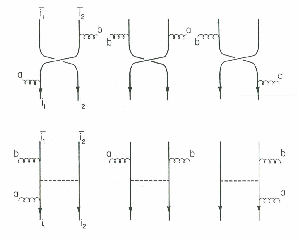
Figure 5: The color flows for quark-antiquark scattering with emission of two gluons.

The color structure in Equation (3.9) has then a very simple physical interpretation. In fact it corresponds to the emission of the gluons off the color-flow lines defined by the functions $D(\{\alpha\})$. Each function $D(\{\alpha\})$ defines a net of color flows, as shown in Figure 5 for the case $m=2$. Each of these color-flow lines, specified by a pair of indices $(i_{k},\mbox{$\bar{\jmath}$}_{k^{\prime}})$, acts as a sort of antenna, that radiates gluons with an associated color factor $(\mbox{$\lambda$}\dots\mbox{$\lambda$})_{i_{k}\,\mbox{${\scriptstyle\bar{\jmath}}$}_{k^{\prime}}}$ (see Figure 5). This color factor is the one appearing in the QED-type diagrams, i.e. diagrams in which all the gauge bosons are emitted from the fermionic line and no three- or four-vector vertices are present. Equation (3.9) shows that even graphs with non-abelian vertices can be decomposed as sums of QED-like diagrams.

Given a helicity configuration for the external states the matrix element for $m$ quark-pair plus $n$ gluon scattering can then be expressed as:

$${\cal M}_{m,n}\;=\;\sum\,\Lambda_{p}(\{n_{i}\},\{\alpha\})\,\tilde{m}^{p}_{\{n_{i}\},\{\alpha\}}(q,h).$$ (3.14)

where the sum is over the permutations of $(j_{1},\dots,j_{m})$. $\Lambda_{p}(\{n_{i}\},\{\alpha\})$ are the color factors appearing in Eq.(3.9): they depend upon the partition and permutation $\{n_{i}\}$ of the gluon indices and upon the antenna pattern determined by the permutation of indices $\{\alpha\}$. We introduced the subscript $p$ to remind that depending on the permutation $\{\alpha\}$ the color factor will be proportional to a given power $N^{-p}$. The sub-amplitudes $\tilde{m}^{p}(q,h)$ multiplying a given color factor are functions of the momenta $q$ and helicities $h$ of the external particles. These sub-amplitudes are obtained by summing contributions from various different Feynman diagrams. If some of the external states are in a given color configuration, for example in a color singlet, the amplitude can be easily obtained by contracting Eq.(3.14) with the proper projector.

To the leading order in $N$ only the terms in the sum with $\alpha_{k}\neq j_{k}$ will contribute, and the sum over colors of the amplitude squared will be the sum of the squares of the functions $\tilde{m}^{p=0}_{\{n_{i}\},\{\alpha\}}$, the interferences being suppressed by negative powers of $N$, as can be easily checked using Eq.(3.8):

$$\sum_{col}|{\cal M}_{m,n}|^{2}\;=\;\mbox{$N^{m+n}$}{\widehat{\sum_{\{n_{i}\}\{\alpha\}}}}\;|m^{0}_{\{n_{i}\},\{\alpha\}}(q,h)|^{2}.$$ (3.15)

The ‘hat’ restricts the sum to the permutations $\{\alpha\}$ with $\alpha_{k}\neq j_{k}$ for all $k$’s.

Each sub-amplitude$~{}m^{p}_{\{n_{i}\},\{\alpha\}}(q,h)$ is invariant under gauge transformations of the gluon polarizations $\epsilon^{i}_{\mu}\rightarrow\epsilon^{i}_{\mu}+\beta p^{i}_{\mu}$. To prove this it is sufficient the orthogonality, to the leading order in $N$, of the color factors. We will now prove this fact.

Let $\delta m^{p}_{\{n_{i}\},\{\alpha\}}(q,h)$ be the gauge variation of a given sub-amplitude. Let $\{\bar{n}_{i}\},\{\bar{\alpha}\}$ be a given partition and a given permutation of quark and gluon indices chosen in such a way that $p=0$. Then the following identity follows:

$$0=\sum_{col}\Lambda^{p=0}_{\{\bar{n}_{i}\},\{\bar{\alpha}\}}(q,h)\delta{\cal M}_{m,n}=N^{n+m}\,\delta m^{0}_{\{\bar{n}_{i}\},\{\bar{\alpha}\}}(q,h)+{\cal O}(1/N^{2}).$$ (3.16)

This shows that all the sub-amplitudes labelled by $p=0$ are gauge-invariant, since gauge-invariance does not depend on $N$ and variations of ${\cal O}(1/\mbox{$N^{2}$})$ cannot cancel the leading piece. We can now select all of the sub-amplitudes corresponding to $p=1$, and repeat the same construction to show that they are gauge invariant too. In this way one can continue until $p=m-1$ is reached, thus proving that each sub-amplitude is in fact gauge invariant.

This gauge invariance is particularly useful for the calculation of the sub-amplitudes, since different gauges can be chosen for different sub-sets of gauge invariant diagrams.

To conclude this Section, we indicate how these color basis generalizes to the case of loop amplitudes. First of all let us remind that loop amplitudes can be obtained by applying proper dispersion relations to tree-level amplitudes, where some of the external particles have been identified and a sum over their possible internal quantum numbers performed. We can then obtain the color form factors which generalize our construction to loop amplitudes by contracting pairs of color indices in the color representations Eqs.(3.1),(3.9).

As an example, let us consider one-loop corrections to the $q\bar{q}g_{1}\dots g_{n}$ process, whose color structure is described at tree-level by Eq.(3.6). For simplicity we will take $n=2$. At one-loop we can have either a gluon contraction (from a $q\bar{q}$ plus four gluon tree diagram), or a quark contraction (from a $q\bar{q}q^{\prime}\bar{q}^{\prime}$ plus two gluon tree diagram). Let us study the gluon loop first: for this we need to consider the color structure of a $q\bar{q}$ plus four gluon tree-level diagram, $(\mbox{$\lambda$}^{a_{1}}\mbox{$\lambda$}^{a_{2}}\dots\mbox{$\lambda$}^{a_{4}})$${}_{i\mbox{${\scriptstyle\bar{\imath}}$}}$. Up to permutations of the indices, we have three possible independent color structures arising from the three inequivalent contractions of gluons:

$$\delta_{cd}(\mbox{$\lambda$}^{a}\mbox{$\lambda$}^{b}\mbox{$\lambda$}^{c}\mbox{$\lambda$}^{d})_{i\mbox{${\scriptstyle\bar{\imath}}$}}\;=\;\delta_{cd}(\mbox{$\lambda$}^{a}\mbox{$\lambda$}^{c}\mbox{$\lambda$}^{d}\mbox{$\lambda$}^{b})_{i\mbox{${\scriptstyle\bar{\imath}}$}}\;=\;{\mbox{$N^{2}$}-1\over\mbox{$N$}}(\mbox{$\lambda$}^{a}\mbox{$\lambda$}^{b})_{i\mbox{${\scriptstyle\bar{\imath}}$}},$$ (3.17)

$$\delta_{cd}(\mbox{$\lambda$}^{c}\mbox{$\lambda$}^{a}\mbox{$\lambda$}^{b}\mbox{$\lambda$}^{d})_{i\mbox{${\scriptstyle\bar{\imath}}$}}\;=\;\delta_{i\mbox{${\scriptstyle\bar{\imath}}$}}\mbox{$tr$}(\mbox{$\lambda$}^{a}\mbox{$\lambda$}^{b})\;-\;{1\over\mbox{$N$}}(\mbox{$\lambda$}^{a}\mbox{$\lambda$}^{b})_{i\mbox{${\scriptstyle\bar{\imath}}$}},$$ (3.18)

$$\delta_{cd}(\mbox{$\lambda$}^{a}\mbox{$\lambda$}^{c}\mbox{$\lambda$}^{b}\mbox{$\lambda$}^{d})_{i\mbox{${\scriptstyle\bar{\imath}}$}}\;=\;{-1\over\mbox{$N$}}(\mbox{$\lambda$}^{a}\mbox{$\lambda$}^{b})_{i\mbox{${\scriptstyle\bar{\imath}}$}}.$$ (3.19)

Two comments are in order: first, a term of the form $\delta_{i\mbox{${\scriptstyle\bar{\imath}}$}}\mbox{$tr$}(\mbox{$\lambda$}^{a}\mbox{$\lambda$}^{b})$, which was absent at tree-level, is now generated. It originates from a color configuration in which the color of the quark flows to the antiquark through the gluon in the loop, without emitting any radiation, while the two external gluons are emitted from the remaining color line circulating in the loop. Since the graph of the color flow is planar and since no trace over internal color lines appears, this term is of order $N^{0}$. The second comment is that each of the sub-amplitudes that correspond to the three color structures (and their permutations):

$$\mbox{$N$}(\mbox{$\lambda$}^{a}\mbox{$\lambda$}^{b})_{i\mbox{${\scriptstyle\bar{\imath}}$}},\quad{-1\over\mbox{$N$}}(\mbox{$\lambda$}^{a}\mbox{$\lambda$}^{b})_{i\mbox{${\scriptstyle\bar{\imath}}$}},\quad\delta_{i\mbox{${\scriptstyle\bar{\imath}}$}}\mbox{$tr$}(\mbox{$\lambda$}^{a}\mbox{$\lambda$}^{b})$$ (3.20)

is gauge invariant. The proof follows the one given above for the tree-level case. Notice that even though the first two color structures are proportional, nevertheless they are independently gauge invariant. Graphically, they correspond to planar and non-planar diagrams, respectively.

From the analysis of the diagrams with a quark contraction, finally, we find again the color form factors given in Eq.(3.20)  plus the form factor $(\mbox{$\lambda$}^{a}\mbox{$\lambda$}^{b})_{i\mbox{${\scriptstyle\bar{\jmath}}$}}$ (from pure quark-loop diagrams).

In the general case of $n$ external gluons and $m$ external quark pairs the possible color form factors can be represented, in a symbolic fashion, by the following expression:

$$\mbox{$N^{p}$}\;\;\mbox{$tr$}(\mbox{$\lambda$}\dots\mbox{$\lambda$})\dots\mbox{$tr$}(\mbox{$\lambda$}\dots\mbox{$\lambda$})\;\delta_{\alpha\bar{\alpha}}\dots\delta_{\beta\bar{\beta}}\;(\mbox{$\lambda$}\dots\mbox{$\lambda$})_{\gamma\bar{\gamma}}\dots(\mbox{$\lambda$}\dots\mbox{$\lambda$})_{\delta\bar{\delta}}.$$ (3.21)

If only external gluons are present, the form factors are given by products of traces of $\lambda$ matrices. In general the power $p$ is an integer, determined by the degree of non-planarity of the given color flow configuration, by the number of closed color lines, and by the number of $U(N)$-trace subtractions. Once again all of the sub-amplitudes relative to a given form factor are gauge invariant. In spite of the proliferation of form factors, which form a highly reducible basis for the color space of a given process, the possibility of breaking the sum of diagrams into many gauge invariant components turns out to be an extremely efficient bookkeeping device to explicitly carry out the calculations of complex matrix elements.

4 Supersymmetry Relations among Amplitudes

The properties of the color form factors introduced in the previous Section only depend on the representation of the gauge group to which the partons belong and to the gauge nature of the couplings, while they are not directly related, for example, to the particle’s spin. By this we mean that the scattering amplitudes for scalar particles transforming as the fundamental representation of $SU(N)$, for example, can be expanded into the same color basis – Equation (3.6) – as the amplitudes for quarks. This expansion will still be gauge invariant and satisfy the important properties illustrated in the previous Section. Likewise, amplitudes with fermions transforming according to the adjoint representation of the gauge group (as in a supersymmetric Yang-Mills theory) can be expanded using the dual basis, Equation (3.1).

In a supersymmetric theory, in which particles with different spins are related to one another by symmetry transformations, the relation between the color structures extends to a relation between the sub-amplitudes as well. This proves to be extremely useful in simplifying the calculations for multi-particle processes in supersymmetric theories, as different amplitudes are connected by simple algebraic identities. In particular, amplitudes with scalars or fermions are much simpler to evaluate than amplitudes with gauge bosons, as the number of diagrams and the complexity of the couplings are smaller in the first case.

The general properties of scattering amplitudes in supersymmetric theories were first discussed by Grisaru et al. in Reference [41, 42]. The importance of these supersymmetry relations for calculations in non-supersymmetric theories was then pointed out in Reference [79], where it was suggested the use on $N=2$ supersymmetry for the evaluation of tree-level multi-gluon processes. As was noticed in Reference [79], in fact, the diagrams contributing to multi-gluon processes at tree-level are exactly the same in the ordinary Yang-Mills theory as they are in its supersymmetric extension, since neither scalar nor fermionic particles are allowed to appear as internal propagators. The amplitudes with only gluons can be related through supersymmetry to easier-to-evaluate amplitudes with scalar and fermion external states, thus significantly simplifying the calculations. $N=1$ supersymmetry was also employed by Kunszt [60] for the calculation of six-parton processes in QCD.

In this Section we will illustrate the basic features of this technique, and we will show how to efficiently complement it with the color expansion developed earlier.

Here we will just use $N=1$ supersymmetry, rather than $N=2$.

One possible representation of $N=1$ supersymmetry contains a massless vector ($g^{\pm}$) and a massless spin $1/2$ Weyl spinor ($\Lambda^{\pm}$). The $\pm$ refers to the two possible helicity states of the vector and the spinor. Let $Q(\eta)$ be the supersymmetry charge [8] with $\eta$ being the fermionic parameter of the transformation. Then $Q(\eta)$ acts on the doublet $(g,\Lambda)$ as follows${}^{\cite[cite]{[\@@bibref{}{susy1,susy2}{}{}]}}$:

$$[Q(\eta),g^{\pm}(p)] = \mp\;\Gamma^{\pm}(p,\eta)\;\Lambda^{\pm},$$ (4.1)

$$[Q(\eta),\Lambda^{\pm}(p)] = \mp\;\Gamma^{\mp}(p,\eta)\;g^{\pm}.$$ (4.2)

$\Gamma^{\pm}(p,\eta)$ is a complex function linear in the anticommuting c-number components of $\eta$ and satisfies:

$$\Gamma^{+}(p,\eta)=[\Gamma^{-}(p,\eta)]^{*}=\bar{\eta}\;u_{-}(p),$$ (4.3)

with $u_{-}(p)$ a negative helicity spinor satisfying the massless Dirac equation with momentum $p$. Because of the arbitrariness in choosing the supersymmetry parameter $\eta$, we choose this to be a negative helicity spinor obeying the Dirac equation with an arbitrary massless momentum $k$ times a Grassmann variable $\theta$. This variable is used to remind us that $\Gamma^{\pm}(p,\eta)$ anti-commutes with the fermion creation and annihilation operators and commutes with the bosonic operators. If we use the notation introduced in the first Section, we then obtain:

$$\Gamma^{+}(p,k)\equiv\Gamma^{+}(p,\eta(k))=\theta\langle k+|p-\rangle\equiv\theta~{}[kp].$$ (4.4)

As a notation, we choose to label the supersymmetry charge $Q(\eta)$ with the momentum $k$ characterising the parameter $\eta$: $Q(k)=Q[\eta(k)]$.

Because of supersymmetry, the operator $Q(k)$ annihilates the vacuum. It follows that the commutator of $Q(k)$ with any string of operators creating or annihilating vectors $g^{\pm}$ and spinors $\Lambda^{\pm}$ has a vanishing vacuum expectation value. If $z_{i}$ represent any of these operators, we then obtain the following Supersymmetry Ward identity (SWI) [41]:

$$0=\langle[Q,\prod_{i=1}^{n}z_{i}]\rangle_{0}=\sum_{i=1}^{n}\langle z_{1}\cdots[Q,z_{i}]\cdots z_{n}\rangle_{0},$$ (4.5)

where $\langle\dots\rangle_{0}$ indicates the vacuum expectation value. If we substitute in equation (4.5) the commutators, we obtain a relation among scattering amplitudes for particles with different spin. General features of Yang-Mills interactions, like helicity conservation in the fermion-fermion-vector vertex guarantee the vanishing of some of the amplitudes in (4.5). The arbitrariness in choosing the reference momentum $k$ for the supersymmetry parameter $\eta$ allows a further simplification of equation  (4.5), by choosing $k$ to be equal to one of the external momenta.

As was first pointed out in Reference [41], these relations can be used to prove general properties of helicity amplitudes in supersymmetric Yang-Mills theories; at tree level, these properties hold for the non-symmetric theory as well. We will here prove some of these properties as an example of the use of the supersymmetry relations. In particular, we will show the vanishing of all the helicity amplitudes of the kind $(\pm\pm\dots\pm)$ and $(\mp\pm\dots\pm)$, where we assume all of the particles as outgoing. For the two-to-two scattering processes in Yang-Mills and gravity, these vanishing theorems were first proved in Reference [95].

Let us start applying the supersymmetry charge to the following string of operators:

$$0 = \langle\left[Q,\Lambda_{1}^{+}g_{2}^{+}g_{3}^{+}\dots g_{n}^{+}\right]\rangle\;=\;-\Gamma^{-}(p_{1},k)~{}A(g_{1}^{+},g_{2}^{+},\dots,g_{n}^{+})~{}+$$ (4.6)

$$+\Gamma^{+}(p_{2},k)~{}A(\Lambda_{1}^{+},\Lambda_{2}^{+},\dots,g_{n}^{+})~{}+~{}\dots~{}+~{}\Gamma^{+}(p_{n},k)~{}A(\Lambda_{1}^{+},g_{2}^{+},\dots,\Lambda_{n}^{+}).$$

Since all of the couplings of fermions to vectors are helicity conserving, all of the amplitudes with two fermions of the same helicity must vanish, and as a consequence of the identity the first term on the right hand side of Equation (4.6) must vanish as well. Therefore maximal helicity violation is forbidden in perturbation theory in any supersymmetric gauge theory, and at tree-level in any gauge theory.

To prove the same theorem for the next helicity violating amplitudes, let us consider the following identity:

$$0 = \langle\left[Q,\Lambda_{1}^{+}g_{2}^{-}g_{3}^{+}\dots g_{n}^{+}\right]\rangle\;=\;$$ (4.7)

$$-~{}\Gamma^{-}(p_{1},k)~{}A(g_{1}^{+},g_{2}^{-},\dots,g_{n}^{+})~{}-~{}\Gamma^{-}(p_{2},k)~{}A(\Lambda_{1}^{+},\Lambda_{2}^{-},\dots,g_{n}^{+}).$$

Here we have omitted all of the vanishing amplitudes with both fermions having the same helicity. Equation (4.7) must be satisfied for any choice of the vector $k$, and in particular we can then choose $k=p_{2}$, proving that the gluonic amplitude must vanish, or $k=p_{1}$, thus proving the vanishing of the amplitudes with the fermion pair.

As a first example of non-vanishing amplitudes, let us now consider the helicity amplitude $(g^{-}_{1},g^{-}_{2},g^{+}_{3},\dots,g^{+}_{n})$, with two negative-helicity gluons and $n-2$ positive-helicity gluons where all of the particles are outgoing. Through the SWI we can relate this amplitude to amplitudes with two fermions and $n-2$ vectors. Helicity conservation for the fermions implies that only an amplitude with one positive- and one negative-helicity gluino can be non-vanishing. In this way equation (4.5) reduces to:

$$\Gamma^{-}(p_{1},k)A(\Lambda^{-}_{1},g^{-}_{2},\Lambda^{+}_{3},g^{+}_{4},\dots,g^{+}_{n}) + \Gamma^{-}(p_{2},k)A(g^{-}_{1},\Lambda^{-}_{2},\Lambda^{+}_{3},g^{+}_{4},\dots,g^{+}_{n})$$ (4.8)

$$- \Gamma^{-}(p_{3},k)A(g^{-}_{1},g^{-}_{2},g^{+}_{3},\dots,g^{+}_{n})=0.$$

Choosing, for example, $k=p_{1}$ we therefore obtain the following relation:

$$A(g^{-}_{1},g^{-}_{2},g^{+}_{3},\dots,g^{+}_{n})\;=\;{\mbox{$\langle 12\rangle$}\over\mbox{$\langle 13\rangle$}}A(g^{-}_{1},\Lambda^{-}_{2},\Lambda^{+}_{3},g^{+}_{4},\dots,g^{+}_{n})$$ (4.9)

As we said before, the purely gluonic amplitudes for the non-supersymmetric and the supersymmetric theory coincide.

It is very important to notice that the supersymmetry identities and all the relations that can be obtained through their use – like the vanishing theorems – hold separately for each of the the sub-amplitudes in which we can expand the full amplitude. This can be easily proved on the basis of gauge invariance and leading order orthogonality of the color form factors.

Another important consequence of the expansion in terms of the color structures described in the previous Section is the possibility of relating directly amplitudes with a pair of quarks to amplitudes with a pair of gluinos. The SWI will then allow us to connect directly amplitudes with only gluons to amplitudes with a quark pair. To make explicit this relation, we remind from the previous Section that amplitudes with a quark pair (gluino pair) can be written in the following way:

$${\cal M}_{n+2}(q,g_{1},\dots,g_{n},\bar{q}) = \sum_{\{1,\dots,n\}}\;(\mbox{$\lambda$}^{a_{1}}\mbox{$\lambda$}^{a_{2}}\dots\mbox{$\lambda$}^{a_{n}})_{i\mbox{${\scriptstyle\bar{\jmath}}$}}\;m_{q}(q,p_{1},\dots,p_{n},\bar{q}),$$ (4.10)

$${\cal M}_{n+2}(g_{1},\dots,g_{n},\Lambda_{n+1},\Lambda_{n+2}) = \sum_{\{1,\dots,n+2\}^{\prime}}\;tr\,(\mbox{$\lambda$}^{a_{1}}\mbox{$\lambda$}^{a_{2}}\dots\mbox{$\lambda$}^{a_{n+2}})\;m_{\Lambda}(p_{1},\dots,p_{n},q_{n+1},q_{n+2}),$$

where the momenta labeled with $q$ are fermion momenta, and where the sub-amplitudes $m_{q}$ and $m_{\Lambda}$ can be found by summing over subsets of Feynman diagrams obtained according to the prescriptions introduced in the previous Section. The prime indicates that only non-cyclic permutations have to be summed over.

The main difference between Equation (4.10) and Equation (4) lies in the fact that while the quark sub-amplitudes $m_{q}$ always have the two fermions adjacent, there are gluino sub-amplitudes with non-adjacent fermions. The gluino sub-amplitudes, furthermore, satisfy the Dual Ward Identity, Equation (3.4). It is easy to prove, by just studying the structure of the relevant Feynman diagrams, that the following identity between quark and gluino amplitudes holds:

$$m_{q}(q,p_{1},\dots,p_{n},\bar{q})\;=\;m_{\Lambda}(q_{n+2},p_{1},\dots,p_{n},q_{n+1}),$$ (4.12)

where $q=q_{n+2}$ and $\bar{q}=q_{n+1}$. The complete proof can be found in Reference [69].

Therefore by just calculating the gluino amplitudes we can automatically obtain the quark amplitudes, using the previous identity, and the purely gluonic amplitudes, by using the SWI. Even if we are only interested in the quark amplitudes, it may still be nevertheless useful to consider the gluino amplitudes with non-adjacent fermions as auxiliary objects, because they satisfy the Dual Ward Identity and can help simplifying expressions.

We will present a complete example of how this works in detail in the next Section, when calculating the five parton processes.

5 Explicit Results

In this Section we will illustrate the use of the various techniques introduced up to now with the explicit calculation of some four- and five-parton processes in a $SU(N)$ massless gauge theory. These results were known since the original papers [26, 78, 40, 61, 73, 18, 32], but reproducing them here will show the simplicity of these techniques and their advantage over the more standard approach. At the end of the section we will collect some results concerning 6-parton processes as well, without going into the explicit details of the calculations. We hope this Section will be helpful to the reader who wants to familiarize himself with the explicit use of these tools.

5.1 Four Partons

As was mentioned in the previous Section it is generally convenient to start the calculations from processes with a pair of fermions and to use the supersymmetry relations to simply obtain the amplitudes of purely gluonic processes as a by-product. The use of the polarization vectors introduced in the first Section and of the dual color basis, however, makes the four gluon calculation so simple by itself that it is useful to just start from it. We will then derive the fermionic amplitude by using the SWI. In the next subsection, when describing the five-parton processes, we will follow the opposite route, as then the fermionic amplitude calculation is considerably simpler than the gluonic one.

We introduce the following notation: $q$ and $\bar{q}$ are the momenta of quark and antiquark, $h_{q}$ is the quark helicity ( the helicity of the antiquark, $h_{\bar{q}}$, is fixed by helicity conservation) and $i,\mbox{$\bar{\imath}$}$ are the color indices; $p_{i},\ (i=1,2,3)$, $h_{i}$ and $a_{i}$ will be respectively the momenta, helicities and colors of the three gluons. All the particles are taken as outgoing, and therefore momentum conservation is given by $q+\bar{q}+\sum p_{i}=0$.

All of the diagrams contributing to the four gluon amplitude have the following color structure:

$$f^{abX}f^{Xcd}\;=\;-tr([\mbox{$\lambda$}^{a},\mbox{$\lambda$}^{b}][\mbox{$\lambda$}^{c},\mbox{$\lambda$}^{d}]).$$ (5.1)

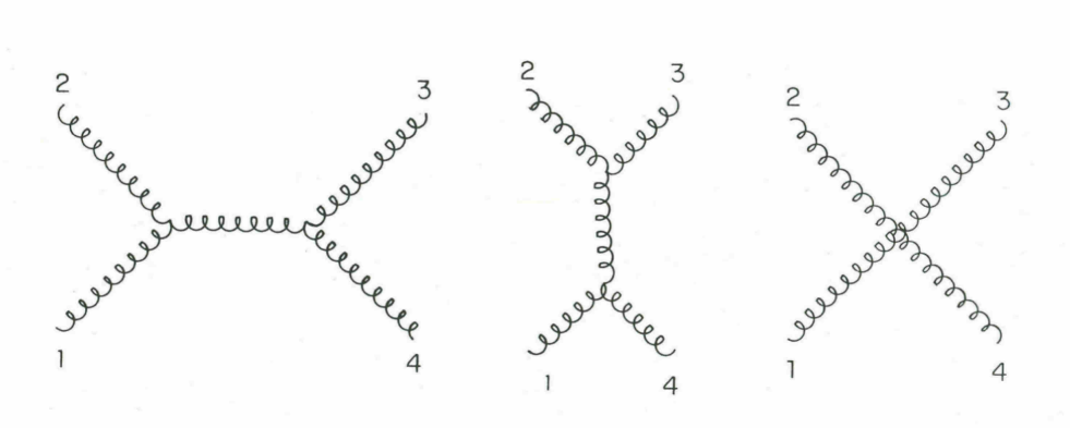
Figure 6: The three diagrams contributing to the subamplitude $m(1,2,3,4)$.

Here we used the normalization conventions introduced in Section 3 . The Feynman rules are given in Appendix C. The Feynman diagrams that enter in the calculation of a given sub-amplitude can just be found by imposing the condition that they contain the trace of the string of $\lambda$ matrices in the proper permutation. For example, when calculating $m(1,2,3,4)$ the only diagrams which will contribute are those drawn in Fig. 6.

Notice that the first diagram will also contribute to the subamplitudes corresponding to the permutations $(1243)$, $(2134)$ and $(2143)$, but remember that for the calculation of the subamplitudes only the kinematical part of the Feynman rules has to be used (see Appendix C). There is only one diagram with the four-gluon coupling, and that contributes to all 6 the permutations.

Before proceeding, let us classify the possible helicity configurations. As it was shown using the supersymmetry relations in the previous Section, the helicity amplitudes with all of the gluons having the same helicity, and the amplitudes with all of the gluons but one having the same helicity are zero. We can prove this independently here by using an explicit representation for the polarization vectors of the gluons, as given in the first Section. In fact, assign to the gluons with the same helicity the same reference momentum, and in the case of sub-amplitudes of the kind $m(\mp,\pm,\dots,\pm)$ fix this reference momentum to be the momentum of the gluon with opposite helicity from the others. Then it is easy to see using the identities given in Appendix A that all of the products $\epsilon^{i}\cdot\epsilon^{j}$ vanish. Since by the Feynman rules (or dimensional analysis) it follows that at tree-level each diagram will contain at least a factor $\epsilon^{i}\cdot\epsilon^{j}$, it follows that these amplitudes will vanish.

Therefore for four-gluon scattering the only non-zero amplitudes will be of the form $(--++)$, up to permutations of the indices. Let us then consider the sub-amplitude $m(1^{-},2^{-},3^{+},4^{+})$, with the reference momenta for the gluons (1,2,3,4) given by the momenta of gluons (3,3,2,2), respectively. For this choice of reference momenta the only non-zero $\epsilon_{i}\cdot\epsilon_{j}$ is $\epsilon_{1}\cdot\epsilon_{4}$. Therefore the only non-zero diagram from Fig. 6  is the first one, which gives explicitly:

$$m(1^{-},2^{-},3^{+},4^{+}) = -2ig^{2}~{}{\epsilon_{1}\cdot\epsilon_{4}~{}~{}\epsilon_{2}\cdot p_{1}~{}\epsilon_{3}\cdot p_{4}\over s_{12}}$$ (5.2)

$$= -ig^{2}~{}{{\langle 12\rangle}^{2}[34]^{2}\over s_{12}~{}s_{23}}\;=\;ig^{2}~{}{\mbox{$\langle 12\rangle$}^{4}\over\mbox{$\langle 12\rangle$}\mbox{$\langle 23\rangle$}\mbox{$\langle 34\rangle$}\mbox{$\langle 41\rangle$}},$$

where various definitions and properties of the spinor dot products collected in the Appendix – together with the kinematical identity $s_{12}$=$s_{34}$ – were used. Notice that even though the diagram containing the $t$-channel exchange vanishes as a consequence of the choice of reference momenta (i.e. the gauge choice), the $t$-pole ($1/s_{23}$) appears from the normalization of the polarization vectors, signalling that the gauge chosen is singular for $s_{23}=0$. This should be expected since, as we pointed out in Section 2 , these gauges are light-cone gauges. Needless to say the result in Eq.(5.2) is gauge invariant.

By using the Dual Ward Identity and the invariance under cyclic permutations we obtain the following identity, which allows us to express the other inequivalent sub-amplitude $m(+-+-)$ in terms of the one we just evaluated using Feynman diagrams:

$$m(1^{-}2^{+}3^{-}4^{+})\;=\;-m(1^{-}3^{-}2^{+}4^{+})-m(3^{-}1^{-}2^{+}4^{+}).$$ (5.3)

Applying the Fierz identity Equation (A.16) to this DWI gives finally:

$$m(1^{-},2^{+},3^{-},4^{+})\;=\;ig^{2}~{}{\mbox{$\langle 13\rangle$}^{4}\over\mbox{$\langle 12\rangle$}\mbox{$\langle 23\rangle$}\mbox{$\langle 34\rangle$}\mbox{$\langle 41\rangle$}},$$ (5.4)

which generalizes to

$$m(1,2,3,4)\;=\;ig^{2}~{}{\mbox{$\langle IJ\rangle$}^{4}\over\mbox{$\langle 12\rangle$}\mbox{$\langle 23\rangle$}\mbox{$\langle 34\rangle$}\mbox{$\langle 41\rangle$}},$$ (5.5)

where $I$ and $J$ are the indices of the negative helicity gluons. The full amplitude will therefore be given by:

$$M(1,2,3,4) = ig^{2}\mbox{$\langle IJ\rangle$}^{4}\sum_{perm^{\prime}}tr(\mbox{$\lambda$}^{a_{1}}\mbox{$\lambda$}^{a_{2}}\mbox{$\lambda$}^{a_{3}}\mbox{$\lambda$}^{a_{4}}){1\over\mbox{$\langle 12\rangle$}\mbox{$\langle 23\rangle$}\mbox{$\langle 34\rangle$}\mbox{$\langle 41\rangle$}}$$

$$= ig^{2}\mbox{$\langle IJ\rangle$}^{4}\sum_{perm^{\prime\prime}}[tr(\mbox{$\lambda$}^{a_{1}}\mbox{$\lambda$}^{a_{2}}\mbox{$\lambda$}^{a_{3}}\mbox{$\lambda$}^{a_{4}})+tr(\mbox{$\lambda$}^{a_{4}}\mbox{$\lambda$}^{a_{3}}\mbox{$\lambda$}^{a_{2}}\mbox{$\lambda$}^{a_{1}})]{1\over\mbox{$\langle 12\rangle$}\mbox{$\langle 23\rangle$}\mbox{$\langle 34\rangle$}\mbox{$\langle 41\rangle$}},$$

where the prime indicates sum over non-cyclic permutations, and the double prime indicates sum over permutations up to cyclic and reverse (i.e. $(1,2,..,n)\rightarrow(n,..,2,1)$ ) re-orderings.

In squaring the four gluon amplitude and summing over colors the ${\cal O}(N^{-2})$ terms in equation (3.5) can be shown to vanish by using only the general properties, especially the Ward Identity, of the sub-amplitude (see Appendix D for the details). Therefore,

$$\sum_{colors}\;|{\cal M}_{4}|^{2}\;=\; {N^{2}(N^{2}-1)}\sum_{perm^{\prime}}|m(1,2,3,4)|^{2},$$ (5.7)

and the square of each sub-amplitude is very simple because the spinor product is the square root of twice the dot product. The final result is the standard four gluon matrix element squared:

$$\sum_{hel.}\sum_{colors}|{\cal M}_{4}|^{2}=N^{2}(N^{2}-1)~{}g^{4}~{}\left(\sum_{i>j}s_{ij}^{4}\right)\sum_{perm^{\prime}}{1\over s_{12}s_{23}s_{34}s_{41}}.$$ (5.8)

Here we have not averaged over helicities or colors.

To obtain the amplitude for two gluons plus a $q\bar{q}$ pair we can use the SWI explicitly given in the previous Section for amplitudes of the kind $M(\mp\mp\pm\dots\pm)$, Eq.(4.9), and we simply get:

$$m(qg_{1}g_{2}\bar{q})\;=\;ig^{2}{\mbox{$\langle qI\rangle$}^{3}\mbox{$\langle\bar{q}I\rangle$}\over\mbox{$\langle\bar{q}q\rangle$}\mbox{$\langle q1\rangle$}\mbox{$\langle 12\rangle$}\mbox{$\langle 2\bar{q}\rangle$}},$$ (5.9)

where we chose the quark and gluon $I$ ($I$=1,2) to have negative helicity, and where $\langle qI\rangle$  is a short-hand for $\langle qp_{I}\rangle$. For a negative helicity anti-quark (i.e. positive helicity quark) it is sufficient to exchange $q$ with $\bar{q}$ in the numerator. The full amplitude will be:

$$M(qg_{1}g_{2}\bar{q})\;=\;ig^{2}{\mbox{$\langle qI\rangle$}^{3}\mbox{$\langle\bar{q}I\rangle$}}\sum_{\{1,2\}}(\mbox{$\lambda$}^{a_{1}}\mbox{$\lambda$}^{a_{2}})_{i{\scriptstyle\bar{\imath}}}{1\over\mbox{$\langle\bar{q}q\rangle$}\mbox{$\langle q1\rangle$}\mbox{$\langle 12\rangle$}\mbox{$\langle 2\bar{q}\rangle$}}$$ (5.10)

with the following square, summed over colors and helicities:

$$\sum_{hel.}\sum_{colors}|{\cal M}_{4}|^{2} = 2N(N^{2}-1)~{}g^{4}~{}\left(\sum_{i=1,2}s_{qi}s_{\bar{q}i}^{3}+s_{qi}^{3}s_{\bar{q}i}\right)\sum_{\{1,2\}}{1\over s_{q\bar{q}}s_{12}s_{q1}s_{\bar{q}2}}$$ (5.11)

$$+ {\cal O}(1/N^{2}).$$

For the details of the squaring and the explicit form of the sub-leading piece, see the Appendix. It is straightforward to check that these results agree with the standard calculations.

5.2 Five Partons

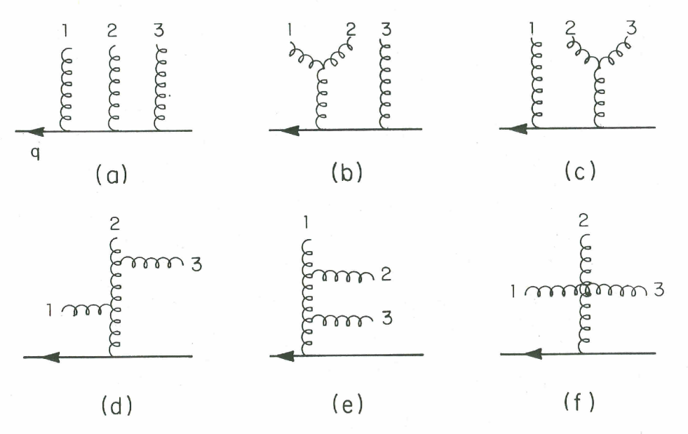
Figure 7: The diagrams contributing to the subamplitude $m(q,1,2,3,\bar{q})$.

We will begin from the calculation of the matrix elements for the scattering of one $q\bar{q}$ pair and three gluons. First of all we classify the possible color form factors for the process. According to Eq.(3.9) these are given by the 6 permutations of the expression $(\mbox{$\lambda$}^{a_{1}}\mbox{$\lambda$}^{a_{2}}\mbox{$\lambda$}^{a_{3}})_{i{\scriptstyle\bar{\imath}}}$. To these six permutations there will correspond six (a priori different) sub-amplitudes. We will consider now the permutation $(1,2,3)$ of the gluon indices, and will show afterwards how to obtain the others by using the various identities introduced previously. Having chosen a color factor, we need to find all of the diagrams which contain this given color factor. For the process under study, these diagrams are shown in Fig. 7). Notice that only the diagram ($a$) contributes exclusively to this sub-amplitude. In fact it is easy to see that, for example, diagram ($b$) will also contribute to the sub-amplitude corresponding to the permutation $(2,1,3)$, diagram ($d$) to $(1,3,2)$, $(2,3,1)$ and $(3,2,1)$, and diagram ($f$) will contribute to all six the permutations. According to our technique, in the calculation of a given sub-amplitude we will just sum up the terms of each diagram proportional to the corresponding permutation.

Now we have to classify the various possible helicity configurations. Up to permutations and charge conjugation, we have four different cases: we can have either all of the three gluons with the same helicity as the quark, or just two, or one, or none. As in the purely gluonic case, amplitudes of the type $M(\mp\pm\dots\pm)$ vanish identically, as was proven using supersymmetry. We will now prove this by using an explicit representation for the polarization vectors.

Let us consider the case where all the gluons have the same helicity, opposite to the helicity of the quark. Let us choose the reference momentum of the gluon polarizations to be the quark momentum. It then follows from Eqs.(A.18) and (A.23):

$$\mbox{$\langle q\pm\!|\,$}\mbox{$\hat{\epsilon}^{\mp}(p_{i},q)$}\;=\;0,\quad\quad\epsilon^{i}\cdot\epsilon^{j}\;=\;0.$$ (5.12)

The bra spinor represents an outgoing quark with helicity $\pm$. Let us then study the branch of gluons starting from the first gluon emitted by the quark leg. The only vector quantities that can contract with the $\gamma$ matrix present at the vertex are the polarization vector of one of the external gluons emitted by this branch, or some combination of momenta of the external gluons themselves. In the first case the diagram is zero because of the first equation above. In the second case, possible only if the branch has more than one external gluon, the saturation of the indices and the dimensionality of the couplings (i.e. there can only be at most one power of momentum for each gluon vertex) forces at least one scalar product between two polarization vectors. In this case the diagram vanishes because of the second identity above. This proof of course extends to tree-level processes with a $q\bar{q}$ pair and an arbitrary number of gluons, and can be easily repeated for the case with all of the gluons having the same helicity, equal to the quark’s one.

Let us now consider the case with two gluons (say 1 and 2) having the helicity opposite to the quark (say +). According to the matching rule discussed in Appendix B, we will choose the reference momentum for the polarizations of gluons 1 and 2 to be the quark momentum $q$, and the reference momentum for the gluon 3 to be the antiquark momentum $\bar{q}$. We then have the following identities:

$$\mbox{$\langle q-\!|\,$}\mbox{$\hat{\epsilon}^{+}(p_{1,2},q)$}\;=\;0,\quad\mbox{$\hat{\epsilon}^{-}(p_{3},\bar{q})$}\mbox{$\,|\bar{q}-\rangle$}\;=\;0,\quad\epsilon^{1}\cdot\epsilon^{2}\;=\;0.$$ (5.13)

Using these identities it is straightforward to show that the only non vanishing diagrams are ($d$) and ($e$). The evaluation of these two diagrams is very simple if use is made of the various identities given in the Appendix A, and leads to the following result for the sub-amplitude:

$$m(q^{-},g_{1}^{-},g_{2}^{+},g_{3}^{+},\bar{q}^{+})\;=\;i\,\mbox{$g_{s}^{3}$}\,{\mbox{$\langle q1\rangle$}^{3}\mbox{$\langle\bar{q}1\rangle$}\over\mbox{$\langle\bar{q}q\rangle$}\mbox{$\langle q1\rangle$}\mbox{$\langle 12\rangle$}\mbox{$\langle 23\rangle$}\mbox{$\langle 3\bar{q}\rangle$}}.$$ (5.14)

Before giving the expressions for the other permutations and helicity combinations, we will use Eq.(5.14)  and the supersymmetry transformation to derive the sub-amplitudes for the five gluon process. The supersymmetry relation that we need is the following:

$$\Gamma^{-}(p_{1},k)m(\Lambda^{-}_{1},g^{-}_{2},\Lambda^{+}_{3},g^{+}_{4},g^{+}_{5}) + \Gamma^{-}(p_{2},k)m(g^{-}_{1},\Lambda^{-}_{2},\Lambda^{+}_{3},g^{+}_{4},g^{+}_{5})$$ (5.15)

$$- \Gamma^{-}(p_{3},k)m(g^{-}_{1},g^{-}_{2},g^{+}_{3},g^{+}_{4},g^{+}_{5})=0.$$

with $\Gamma^{-}(p,k)=\mbox{$\langle pk\rangle$}$ and $\Lambda$ being the fermion field. The second sub-amplitude entering this identity corresponds to the quark amplitude we just calculated, as was mentioned in the previous Section, while the first term is one of the fermionic sub-amplitudes that would be necessary for the calculation of amplitudes with fermions in the adjoint representation. By choosing $k=p_{1}$ we can exclude this term, and using Eq.(5.14) we directly obtain:

$$m(g_{1}^{-},g_{2}^{-},g_{3}^{+},g_{4}^{+},g_{5}^{+})\;=\;i\,\mbox{$g_{s}^{3}$}\,{\mbox{$\langle 12\rangle$}^{4}\over\mbox{$\langle 12\rangle$}\mbox{$\langle 23\rangle$}\mbox{$\langle 34\rangle$}\mbox{$\langle 45\rangle$}\mbox{$\langle 51\rangle$}}.$$ (5.16)

To get the sub-amplitudes for the other permutations, we only need to use the symmetry of the sub-amplitude under exchange of identical bosons and the repeated application of the Fierz relation (Eq.(A.16)) on the Dual Ward Identity :

$$\sum_{cycl(1,..,4)}m(1,2,3,4,5)\;=\;0,$$ (5.17)

the sum being over the 4 cyclic permutations of $(1,2,3,4)$. One easily obtains:

$$m(g_{1},g_{2},g_{3},g_{4},g_{5})\;=\;i\,\mbox{$g_{s}^{3}$}\,{\mbox{$\langle IJ\rangle$}^{4}\over\mbox{$\langle 12\rangle$}\mbox{$\langle 23\rangle$}\mbox{$\langle 34\rangle$}\mbox{$\langle 45\rangle$}\mbox{$\langle 51\rangle$}},$$ (5.18)

where $I$ and $J$ are the momenta of the two gluons with the same (negative) helicity. By using again now Eq.(5.15) one then obtains the expression for the general permutation of the fermionic sub-amplitude:

$$m(q^{-},g_{1},g_{2},g_{3},\bar{q}^{+})\;=\;i\,\mbox{$g_{s}^{3}$}\,{\mbox{$\langle qI\rangle$}^{3}\mbox{$\langle\bar{q}I\rangle$}\over\mbox{$\langle\bar{q}q\rangle$}\mbox{$\langle q1\rangle$}\mbox{$\langle 12\rangle$}\mbox{$\langle 23\rangle$}\mbox{$\langle 3\bar{q}\rangle$}},$$ (5.19)

where now $I$ is the index of the only gluon with negative helicity. Similarly, the sub-amplitude for the helicity configuration with one negative helicity gluon and a negative helicity antiquark is given by:

$$m(q^{+},g_{1},g_{2},g_{3},\bar{q}^{-})\;=\;i\,\mbox{$g_{s}^{3}$}\,{\mbox{$\langle qI\rangle$}\mbox{$\langle\bar{q}I\rangle$}^{3}\over\mbox{$\langle\bar{q}q\rangle$}\mbox{$\langle q1\rangle$}\mbox{$\langle 12\rangle$}\mbox{$\langle 23\rangle$}\mbox{$\langle 3\bar{q}\rangle$}}.$$ (5.20)

All of the sub-amplitudes for the processes with opposite helicities (i.e. $(++---)$) can be obtained from the previous expressions by replacing $\langle\ \rangle$  products with $[\ ]$  products.

Squaring the full amplitude and summing over colors and helicity configurations, we then obtain:

$$|M(g_{1},\dots,g_{5})|^{2}\;=\; 2\mbox{$g_{s}^{6}$}\mbox{$N^{3}$}(\mbox{$N^{2}$}-1)\sum_{i>j}s_{ij}^{4}\;\sum\;{1\over s_{12}s_{23}s_{34}s_{45}s_{51}},$$ (5.22)

$$|M(q,\bar{q},g_{1},g_{2},g_{3})|^{2}\;=\; 2\mbox{$g_{s}^{6}$}\mbox{$N^{2}$}(\mbox{$N^{2}$}-1)\sum_{i}(s_{qi}^{3}s_{\bar{q}i}\;+\;s_{qi}s_{\bar{q}i}^{3})$$

$$\sum_{\{1,2,3\}}\;{1\over s_{q\bar{q}}s_{q1}s_{12}s_{23}s_{3\bar{q}}}\;+\;O(N^{-2}).$$

For the details of the squaring of the color part, see Appendix D.

5.3 Six Partons

The six-parton processes are more complex: two independent sets of helicity amplitudes are needed: ${\cal}M_{2-4+}$ and ${\cal M}_{3-3+}$. The first ones are a trivial generalization of the five-parton amplitudes, and are given in the case of two quark-four gluon and six gluons, respectively, by:

$${\cal M}(\bar{q}^{+}_{1},q^{-}_{2},g^{-}_{3},g^{+}_{4},\dots,g^{+}_{6})=ig^{4}\langle 23\rangle^{3}\langle 13\rangle\sum_{\{3,4,5,6\}}\;(\lambda^{3}\lambda^{4}\lambda^{5}\lambda^{6})_{\hat{2}\hat{1}}\;{1\over\langle 12\rangle\langle 23\rangle\cdots\langle 61\rangle}.$$ (5.23)

$${\cal M}(g^{-}_{1},g^{-}_{2},g^{+}_{3},g^{+}_{4},\dots,g^{+}_{6})=ig^{4}\langle 12\rangle^{4}\sum_{\{1,2,3,4,5,6\}^{\prime}}\;tr(\mbox{$\lambda$}^{a_{1}}\mbox{$\lambda$}^{a_{2}}\dots\mbox{$\lambda$}^{a_{6}})\;{1\over\langle 12\rangle\langle 23\rangle\cdots\langle 61\rangle},$$ (5.24)

These sub-amplitudes can be shown to satisfy all of the required properties, such as the SWI, the Dual Ward Identity and the proper soft and collinear factorization (see Section 6 ). At the leading order in $N$ the sum of these matrix elements squared, summed over colors and over the configurations with helicities $(--++++)$ and $(++----)$, can be easily obtained using the properties of the $\lambda$ matrices, giving:

$$|M(g_{1},\dots,g_{6})|^{2}\;=\;2\mbox{$g_{s}^{8}$}\mbox{$N^{4}$}(\mbox{$N^{2}$}-1)\sum_{i>j}s_{ij}^{4}\;\sum\;{1\over s_{12}s_{23}\cdots s_{61}}\;+\;O(N^{-2}),\\ \ \$$

$$|M(q,\bar{q},g_{1},g_{2},g_{3},g_{4})|^{2}\;=\; 2\mbox{$g_{s}^{8}$}\mbox{$N^{3}$}(\mbox{$N^{2}$}-1)\sum_{i}(s_{qi}^{3}s_{\bar{q}i}\;+\;s_{qi}s_{\bar{q}i}^{3})$$ (5.25)

$$\sum_{\{1,2,3,4\}}\;{1\over s_{q\bar{q}}s_{q1}s_{12}s_{23}s_{34}s_{4\bar{q}}}\;+\;O(N^{-2}).$$

Notice that contrarily to the 4- and 5-gluon case, here the 6-gluon amplitude squared has a non-vanishing contribution at the sub-leading order in $N$. Its precise form is given in Appendix D. Using the factorization properties of the amplitude, however, it is easy to check that this sub-leading terms do not have collinear divergencies [66]. The absence of these enhancement factors makes the numerical value of these sub-leading terms even smaller than what one would naively expect from the simple $1/N^{2}$ suppression. This fact will be discussed in more detail in Section 10 , where we will illustrate some techniques to approximate the multi-parton matrix elements.

The six-parton helicity amplitudes ${\cal M}_{3-3+}$ is described by three distinct sub-amplitudes, characterised by three inequivalent helicity orderings: $(+++---)$, $(++-+--)$ and $(+-+-+-)$. Because of duality, as explained in Ref.[51], all of these sub-amplitudes can be written in the following form:

$$m(1,2,\dots,6) = ig^{4}\left[{P_{1}\over t_{123}s_{12}s_{23}s_{45}s_{56}}~{}+~{}{P_{2}\over t_{234}s_{23}s_{34}s_{56}s_{61}}\right.$$ (5.26)

$$~{}+~{} {P_{3}\over t_{345}s_{34}s_{45}s_{61}s_{12}}~{}+~{}\left.{P_{s}\over{s_{12}s_{23}s_{34}s_{45}s_{56}s_{61}}}~{}\right].$$

where $t_{ijk}\equiv(p_{i}+p_{j}+p_{k})^{2}~{}=~{}s_{ij}+s_{jk}+s_{ki}$. The coefficients $P_{i}$ will depend on the particular helicity configuration and on the process (6-gluons or 2-quark plus four-gluons). For the purely gluonic case, a further relation can be found between the $P$’s that will reduce Eq.(5.26) to [67]:

$$m_{3+3-}(g_{1},g_{2},\dots,g_{6})\;=\;ig^{4}\left[{\alpha^{2}\over t_{123}s_{12}s_{23}s_{45}s_{56}}~{}+~{}{\beta^{2}\over t_{234}s_{23}s_{34}s_{56}s_{61}}\right.$$

$$~{}+~{}{\gamma^{2}\over t_{345}s_{34}s_{45}s_{61}s_{12}}~{}+~{}\left.{{t_{123}\beta\gamma~{}+~{}t_{234}\gamma\alpha~{}+~{}t_{345}\alpha\beta}\over{s_{12}s_{23}s_{34}s_{45}s_{56}s_{61}}}~{}\right],$$ (5.27)

For reference, we give the coefficients $P_{i}$’s and $\alpha,\beta,\gamma$ in Table 2-3 and Table 4, respectively, without derivation. Here we will just show how to relate the two sets of coefficients, for the purely gluonic and the $q\bar{q}$ plus gluons case, using the various identities introduced in the previous Sections. For simplicity we will just work with the $(---+++)$ helicity ordering, but the same construction can be repeated for the other orderings as well.

Suppose we have calculated the fermionic amplitudes; then it is easy to prove the following identity, using a proper SWI:

$$\mbox{$[36]$}m(g^{-}_{1},g^{-}_{2},g^{-}_{3},g^{+}_{4},g^{+}_{5},g^{+}_{6}) = -\mbox{$[31]$}m(\Lambda^{+}_{6},\Lambda^{-}_{1},g^{-}_{2},g^{-}_{3},g^{+}_{4},g^{+}_{5})$$ (5.28)

$$-\mbox{$[32]$}m(\Lambda^{+}_{6},g^{-}_{1},\Lambda^{-}_{2},g^{-}_{3},g^{+}_{4},g^{+}_{5}).$$

Here by $\Lambda$ we refer to a generic fermion, $q$ or $\bar{q}$. Helicity conservation has been used to cancel the two amplitudes with two negative-helicity fermions, and the Grassmannian nature of $\Gamma^{\pm}$ was used when moving it through $\Lambda_{2}$. The amplitude with the non-adjacent fermions can be extracted by using the Dual Ward Identity obtained by moving the gluon 1 :

$$m(\Lambda^{+}_{1},g^{-}_{2},\Lambda^{-}_{3},g^{-}_{4},g^{+}_{5},g^{+}_{6}) =$$

$$-m(\Lambda^{+}_{1},\Lambda^{-}_{3},g^{-}_{2},g^{-}_{4},g^{+}_{5},g^{+}_{6}) - m(\Lambda^{+}_{1},\Lambda^{-}_{3},g^{-}_{4},g^{-}_{2},g^{+}_{5},g^{+}_{6})$$

$$-m(\Lambda^{+}_{1},\Lambda^{-}_{3},g^{-}_{4},g^{+}_{5},g^{-}_{2},g^{+}_{6}) - m(\Lambda^{+}_{1},\Lambda^{-}_{3},g^{-}_{4},g^{+}_{5},g^{+}_{6},g^{-}_{2}).$$ (5.29)

Therefore the knowledge of the fermionic amplitudes is completely sufficient to obtain the purely gluonic ones without having to calculate any additional Feynman diagram. In particular, if one were just interested in the numerical value of the amplitudes to calculate scattering processes, one could just use the previous equations as operative definitions of the gluonic amplitudes, without having to go through the algebra necessary to find explicit expressions.

	$P_{1}$	$P_{2}$	$P_{3}$
$(g_{3},g_{4},g_{5},g_{6})$	$U=p_{1}~{}+~{}p_{2}~{}+~{}p_{3}$	$V=p_{2}~{}+~{}p_{3}~{}+~{}p_{4}$	$W=p_{3}~{}+~{}p_{4}~{}+~{}p_{5}$
$(-,-,+,+)_{(I)}$	${}[56]^{2}\langle 13\rangle\langle 23\rangle\langle 1|U|4\rangle^{2}$	0	$-[16][26]\langle 34\rangle^{2}\langle 5|W|2\rangle^{2}$
$(+,+,-,-)_{(II)}$	$-[13][23]\langle 56\rangle^{2}\langle 4|U|2\rangle^{2}$	0	${}[34]^{2}\langle 16\rangle\langle 26\rangle\langle 1|W|5\rangle^{2}$
$(-,+,+,-)_{(III)}$	${}[45]^{2}\langle 13\rangle\langle 23\rangle\langle 1|U|6\rangle^{2}$	${}[15]\langle 23\rangle\langle 5|V|3\rangle\langle 4|V|6\rangle^{2}$	${}[45]^{2}\langle 16\rangle\langle 26\rangle\langle 1|W|3\rangle^{2}$
$(+,-,-,+)_{(IV)}$	$-\langle 45\rangle^{2}[13][23]\langle 6|U|2\rangle^{2}$	${}[16]\langle 24\rangle\langle 6|V|4\rangle\langle 3|V|5\rangle^{2}$	$-\langle 45\rangle^{2}[16][26]\langle 3|W|2\rangle^{2}$
$(-,+,-,+,)_{(V)}$	${}[46]^{2}\langle 13\rangle\langle 23\rangle\langle 1|U|5\rangle^{2}$	${}[16]\langle 23\rangle\langle 6|V|3\rangle\langle 4|V|5\rangle^{2}$	$-[16]{}[26]\langle 35\rangle^{2}\langle 4|W|2\rangle^{2}$
$(+,-,+,-,)_{(VI)}$	$-[13][23]\langle 46\rangle^{2}\langle 5|U|2\rangle^{2}$	${}[15]\langle 24\rangle\langle 5|V|4\rangle\langle 3|V|6\rangle^{2}$	${}[35]^{2}\langle 16\rangle\langle 26\rangle\langle 1|W|4\rangle^{2}$

Table 2: The numerator functions $P_{i}$ for $m(\bar{q}^{+}_{1},q^{-}_{2},g_{3},g_{4},g_{5},g_{6})$. The left column contains the helicity orderings of the gluons we define $\langle I|K|J\rangle\equiv\langle I+|K\cdot\gamma|J+\rangle$.

$(g_{3},g_{4},g_{5},g_{6})$	$P_{s}$
$(-,-,+,+)_{(I)}$	$\langle 23\rangle\langle 34\rangle[56][61]\left(\langle 1|U|4\rangle\langle 2|V|1\rangle\langle 5|W|2\rangle-S_{56}[23]\langle 34\rangle\langle 5|W|2\rangle-S_{34}[56]\langle 61\rangle\langle 1|U|4\rangle\right)$
$(+,+,-,-)_{(II)}$	$[23][34]\langle 56\rangle\langle 61\rangle\langle 4|U|2\rangle\langle 1|V|2\rangle\langle 1|W|5\rangle$
$(-,+,+,-)_{(III)}$	$-t_{123}[15][45]\langle 13\rangle\langle 26\rangle\langle 4|V|6\rangle\langle 1|W|3\rangle-t_{234}[45]^{2}\langle 13\rangle\langle 26\rangle\langle 1|U|6\rangle\langle 1|W|3\rangle$
	$+t_{345}[15][45]\langle 13\rangle\langle 23\rangle\langle 1|U|6\rangle\langle 4|V|6\rangle+[45][56]\langle 12\rangle\langle 36\rangle\langle 1|U|6\rangle\langle 4|V|6\rangle\langle 1|W|3\rangle$
$(+,-,-,+)_{(IV)}$	$t_{123}[16][26]\langle 24\rangle\langle 45\rangle\langle 3|V|5\rangle\langle 3|W|2\rangle+t_{234}[13][26]\langle 45\rangle^{2}\langle 6|U|2\rangle\langle 3|W|2\rangle$
	$-t_{345}[13][26]\langle 24\rangle\langle 45\rangle\langle 6|U|2\rangle\langle 3|V|5\rangle+[12][36]\langle 34\rangle\langle 45\rangle\langle 6|U|2\rangle\langle 3|V|5\rangle\langle 3|W|2\rangle$
$(-,+,-,+)_{(V)}$	$-t_{123}[16]\langle 35\rangle\langle 6|V|3\rangle\langle 4|V|5\rangle\langle 4|W|2\rangle-t_{234}[46]\langle 35\rangle\langle 6|V|3\rangle\langle 1|U|5\rangle\langle 4|W|2\rangle$
	$+t_{345}[46]\langle 23\rangle\langle 6|V|3\rangle\langle 1|U|5\rangle\langle 4|V|5\rangle-[46][56]\langle 34\rangle\langle 35\rangle\langle 1|U|5\rangle\langle 4|V|5\rangle\langle 4|W|2\rangle$
$(+,-,+,-)_{(VI)}$	$[12][23][15][35]\langle 14\rangle\langle 24\rangle\langle 26\rangle\langle 56\rangle\langle 5|U|2\rangle+(S_{12}S_{23}-S_{12}S_{45})[15][35]\langle 24\rangle\langle 46\rangle\langle 3|V|6\rangle$
	$-S_{23}S_{16}[35]^{2}\langle 26\rangle\langle 46\rangle\langle 1|W|4\rangle-[15]^{2}[23][34]\langle 12\rangle\langle 16\rangle\langle 24\rangle\langle 46\rangle\langle 1|W|4\rangle$
	$+S_{23}S_{16}[15][35]\langle 46\rangle^{2}\langle 3|1+5|2\rangle+S_{12}S_{15}[15][23][35]\langle 24\rangle\langle 26\rangle\langle 46\rangle$

Table 3: The numerator functions $P_{s}$ for $m(\bar{q}^{+}_{1},q^{-}_{2},g_{3},g_{4},g_{5},g_{6})$ with the same notation as Table 1.

The squaring of the amplitudes is independent of the particular helicity configurations, and the explicit formulas for leading and sub-leading terms are given in Appendix D. The same consideration concerning the collinear finiteness of the sub-leading piece made before for the helicities $(--++++)$ also holds here.

	$1^{+}2^{+}3^{+}4^{-}5^{-}6^{-}$	$1^{+}2^{+}3^{-}4^{+}5^{-}6^{-}$	$1^{+}2^{-}3^{+}4^{-}5^{+}6^{-}$
	$X=p_{1}+p_{2}+p_{3}$	$Y=p_{1}+p_{2}+p_{4}$	$Z=p_{1}+p_{3}+p_{5}$
$\bf\alpha$	0	$-[12]\langle 56\rangle\langle 4|Y|3\rangle$	$[13]\langle 46\rangle\langle 5|Z|2\rangle$
$\bf\beta$	$[23]\langle 56\rangle\langle 1|X|4\rangle$	$[24]\langle 56\rangle\langle 1|Y|3\rangle$	$[51]\langle 24\rangle\langle 3|Z|6\rangle$
$\bf\gamma$	$[12]\langle 45\rangle\langle 3|X|6\rangle$	$[12]\langle 35\rangle\langle 4|Y|6\rangle$	$[35]\langle 62\rangle\langle 1|Z|4\rangle$

Table 4: Coefficients for the $m_{3+3-}(g_{1},g_{2},g_{3},g_{4},g_{5},g_{6})$ sub-amplitudes. We define $\langle I|K|J\rangle\equiv\langle I+|K\cdot\gamma|J+\rangle$

6 Factorization Properties of Dual Amplitudes

One of the most important properties of the dual amplitudes, which partly accounts for the relative simplicity of their explicit expressions, is their factorizability on multi-particle poles. The residues at these poles are determined by unitarity, and can be expressed in terms of dual amplitudes for processes with a smaller number of external particles. The possibility of factorizing these amplitudes into products of amplitudes and near-the-pole propagators, puts such severe constraints on the amplitudes themselves that often it is possible to deduce their explicit form by just imposing unitarity and Lorentz invariance. Subtle cancellations which usually are made explicit only at the matrix element square level for the full amplitude, here are made manifest at the matrix element level for each single dual amplitude. From the technical point of view, the constraints imposed by factorizability provide furthermore a powerful check all along the way while performing complex calculations.

A very simple and instructive way to prove these factorization properties [68] is by using the Koba-Nielsen representation for the amplitudes [56, 86]. While this representation may not be too helpful in carrying out explicit calculations, this compact symbolic representation provides a powerful tool for deriving general properties of the amplitudes. It was used independently by Lipatov in Ref. [63] to study the emission of soft gluons and gravitons, in Ref. [64] to study the production of gluons in tachyon-tachyon scattering and by Fadin and Lipatov in Ref. [35] to describe multi-gluon production in a quasi-multi-Regge kinematics, in which all the pairs of final state paticles except one have large invariant mass and fixed transverse momentum.

The following factorization properties can also be proved in a simple and effective way [13] by using the recursive relations introduced by Berends and Giele [12] and reviewed here in the following Section (see also Ref.[58] for a derivation of the recursive relations using the Koba-Nielsen representation of the amplitudes. and further applications of this approach).

For the sake of definiteness we will deal in this Section with gluonic amplitudes only. As was mentioned previously, an $n$-gluon dual amplitude can be represented by considering the terms with lowest momentum dimensionality ($[P]^{4-n}$) in the expansion of the following expression:

$$m_{n}(k_{1},\epsilon_{1};k_{2},\epsilon_{2};\dots;k_{n},\epsilon_{n}) = \int_{z_{1}<z_{2}<\dots<z_{n}}\;\prod_{i=3}^{n-1}\mbox{d}{z_{i}}\;\mu_{KN}\;\prod_{n\geq i>j\geq 1}\;(z_{i}-z_{j})^{k_{i}k_{j}}\;$$ (6.1)

$$\exp\left\{\sum_{i\neq j}{1\over 2}\,{\epsilon_{i}\epsilon_{j}\over(z_{i}-z_{j})^{2}}\;+\;{k_{i}\epsilon_{j}\over(z_{i}-z_{j})}\right\},$$

where $\mu_{KN}=(z_{2}-z_{1})(z_{n}-z_{1})(z_{n}-z_{2})$ is the measure that makes the integral invariant under Moebius transformations. The values of $z_{1,2,n}$ can be chosen arbitrarily, but usually as follows: $z_{1}=0$, $z_{2}=1$ and $z_{n}=\infty$. The gluon amplitude is given by the terms in the expansion of the Koba-Nielsen expression which are multi-linear in the polarization vectors $\epsilon_{i}$.

The singularities of the matrix elements arise from the regions of integration where two or more $z$’s coalesce. This follows easily from Eq.(6.1); for example, it is easy to check that poles like $1/(k_{i}+k_{j}+\dots+k_{l})^{2}$ arise from the region of integration $z_{i}\sim z_{j}\sim\dots\sim z_{l}$. From this it follows that for a given dual amplitude, represented by a determined permutation of the indices, the only singularities that can appear are multi-particle poles in which the indices of the momenta have to appear consequently within the given permutation.

6.1 Soft Gluon Factorization

Let us start from the simplest kind of singularities, i.e. those due to the emission of soft gluons. We want to show that when one of the gluons becomes soft (i.e. $p\rightarrow 0$) the dual amplitude can be written as the product of a dual amplitude describing the process involving the remaining gluons times an overall factor.

Let us introduce the following conventions: we will indicate with $w$ the $z$ coordinate of the soft gluon, with $p$ its momentum and with $\zeta$ its polarization. We will take the permutation in which the soft gluon is, by convention, inserted between gluon 1 and gluon 2. We will furthermore fix the values of $z_{1,2,n}$ as given above, and therefore will integrate the soft gluon ’coordinate’ $w$ in the range $z_{1}=0\leq w\leq z_{2}=1$.

It is then simple to prove that in the $p\rightarrow 0$ approximation the Koba-Nielsen formula becomes:

$$m_{n+1}(k_{1},\epsilon_{1};p,\zeta;k_{2},\epsilon_{2};\dots;k_{n},\epsilon_{n})\;=\;\int_{0}^{1}\mbox{d}{w}\;w^{pk_{1}}(1-w)^{pk_{2}}\int_{z_{1}<w<z_{2}<\dots<z_{n}}\;\bar{Z}\;\bar{E}\;$$

$$\exp\left\{{\epsilon_{1}\zeta\over w^{2}}+{\epsilon_{2}\zeta\over(1-w)^{2}}-{k_{1}\zeta\over w}+{k_{2}\zeta\over(1-w)}+\zeta\cdot\sum_{i>2}({\epsilon_{i}\over(z_{i}-w)^{2}}-{k_{i}\over(z_{i}-w)})\right\},$$ (6.2)

where

$$\bar{Z} = \prod_{i=3}^{n-1}\mbox{d}{z_{i}}\;\mu_{KN}\;\prod_{n\geq i>j\geq 1}\;(z_{i}-z_{j})^{k_{i}k_{j}}\;$$ (6.3)

$$\bar{E} = \exp\left\{\sum_{i\neq j}{1\over 2}\,{\epsilon_{i}\epsilon_{j}\over(z_{i}-z_{j})^{2}}\;+\;{k_{i}\epsilon_{j}\over(z_{i}-z_{j})}\right\}.$$ (6.4)

The momentum $p$ was kept only in those terms which can give rise to singularities. By expanding at the linear level in the polarizations, we will now find integrals in $w$ of the following form:

$$I(a,b) = \int_{0}^{1}\mbox{d}{w}\;w^{pk_{1}}(1-w)^{pk_{2}}\;w^{-a}(1-w)^{-b}$$ (6.5)

$$= {\Gamma(-a+1+pk_{1})\Gamma(-b+1+pk_{2})\over\Gamma(pk_{1}+pk_{2}+2-a-b)}.$$

where the pair $a,b$ can take the following values: $(a=0,1,2;b=0)$ or $(a=0;b=0,1,2)$. The only integrals which give the leading infrared singularities are $I(1,0)$ and $I(0,1)$, which in the soft limit behave, respectively, like $1/pk_{1}$ and $1/pk_{2}$. Therefore the dual amplitude corresponding to the emission of a soft gluon takes the following form:

$$m_{n+1}(k_{1},\epsilon_{1};p,\zeta;k_{2},\epsilon_{2};\dots;k_{n},\epsilon_{n}) = \left[\zeta\cdot({k_{2}\over pk_{2}}-{k_{1}\over pk_{1}})\right]m_{n}(k_{1},\epsilon_{1};k_{2},\epsilon_{2};\dots;k_{n},\epsilon_{n})$$ (6.6)

$$\equiv \zeta\cdot j_{eik}~{}m_{n},$$

where $j_{eik}$ is the classical gauge invariant eikonal current. Because of gauge invariance, we can use the spinorial representation of the polarization $\zeta$ with an arbitrary reference momentum – say $k_{2}$. For a positive-helicity soft gluon, we find the following result:

$$\zeta\cdot j_{eik}\;=\;{\mbox{$\langle p\,\!|\,$}k_{2}\mbox{$\,|k_{1}\rangle$}\over\sqrt{2}\;\mbox{$\langle k_{1}p\rangle$}(pk_{2})}\;=\;\sqrt{2}{\mbox{$\langle 12\rangle$}\over\mbox{$\langle 1p\rangle$}\mbox{$\langle p2\rangle$}},$$ (6.7)

which is the square root of the usual eikonal factor:

$$|\zeta\cdot j_{eik}|^{2}\;=\;{(12)\over(p1)(p2)}.$$ (6.8)

For the emission of a negative-helicity gluon we just have to change the $\langle ij\rangle$  products with $[ji]$ products. The factorization of the sub-amplitude, Eq.(6.6), does not imply the eikonalization of the full matrix element, as is the case in QED, because of the convolution with the color Chan-Paton factors: the interference of gluons in the non-abelian theory persists in the soft limit. Repeated applications of Eq.(6.6) lead to the multi-gluon amplitudes introduced in [10]. The properties of the sub-amplitudes in presence of soft-gluon emission were also studied in detail by Berends and Giele in Ref.[13]. Here expressions were given for the case of multiple soft emission, in the case were soft gluons are strongly ordered in energy $(E_{1}>>E_{2}>>\dots)$, and in the case in which energies are not strongly ordered $(E_{1}\sim E_{2}\dots\sim E_{k}<<E_{k+1}\dots)$. We refer to that paper for the details.

6.2 Factorization of Collinear Poles

In a similar fashion one can analyze the factorization properties of the amplitudes near a collinear singularity by studying the residues of the appropriate poles in the Koba-Nielsen variables. To this end, we will assume that the collinear pair is formed by the first two gluons, and will label the variables in the following fashion: the first two gluons will have momenta $p_{1}$ and $p_{2}$, respectively, and polarizations $\zeta_{1,2}$. Their Koba-Nielsen variables will be $w_{1}$ and $w_{2}$. For the remaining $n$ gluons we will use the notation $k_{i}$, $\epsilon_{i}$ and $z_{i}$ for momentum, polarization and Koba-Nielsen coordinate, respectively. Furthermore we will fix the range of the Koba-Nielsen integration as follows:

$$w_{1}=0\;<\;w_{2}=w\;<\;z_{1}=1\;<\;\dots\;<\;z_{n}\rightarrow\infty.$$ (6.9)

The collinear singularity – $1/(p_{1}p_{2})$ – will arise from the region $w\rightarrow 0$. To isolate the leading contributions, therefore, we will expand the KN integral in a Laurent series in $w$, keeping only the singular part:

$$m_{n+2}(p_{1},p_{2},k_{1},\dots,k_{n})\;=\;\int_{0}^{1}\mbox{d}{w}\;w^{p_{1}p_{2}}\prod_{i=1}^{n}z_{i}^{Pk_{i}}\;\left(1-w\sum{p_{2}k_{i}\over z_{i}}\right)\;\exp(-P\sum{\epsilon_{i}\over z_{i}})$$

$$\int_{i=2,n-1}\mbox{d}{z_{i}}\;\bar{Z}\bar{E}\;\left\{{\zeta_{1}\zeta_{2}\over w^{2}}\ -{1\over w}\left[(\zeta_{1}\zeta_{2})p_{2}^{\mu}+(p_{1}\zeta_{2})\zeta_{1}^{\mu}-(p_{2}\zeta_{1})\zeta_{2}^{\mu}\right]\sum({\epsilon_{i}^{\mu}\over z_{i}^{2}}+{k_{i}^{\mu}\over z_{i}})\right\},$$ (6.10)

where $\bar{E}$ and $\bar{Z}$ were defined above, and where $P=p_{1}+p_{2}$. We left out terms like $(p_{1}\zeta_{2})(p_{2}\zeta_{1})$ because they have higher dimension (i.e. they would disappear in the zero slope limit, in the string theory language). The integrals in $w$ can be regularized by introducing a factor $(1-w)^{\epsilon}$, which allows them to be defined in terms of Euler functions by analytic continuation, and then taking the $\epsilon\rightarrow 0$ limit. In this way only the integral in $w^{(p_{1}p_{2}-1)}$ contributes to the leading behaviour.

By performing the integrations and keeping only the leading terms, we obtain the following expression:

$$m_{n+2}(p_{1},p_{2},k_{1},\dots,k_{n})\;=\;\int\prod_{i=2,n-1}\mbox{d}{z_{i}}\;\bar{Z}\bar{E}\;\prod_{i=1}^{n}z_{i}^{Pk_{i}}\;{-1\over 2(p_{1}p_{2})}\;\exp(-P\sum{\epsilon_{i}\over z_{i}})$$

$$\left\{(\zeta_{1}\zeta_{2})P_{\mu}\sum({\epsilon_{i}^{\mu}\over z_{i}^{2}}+{k_{i}^{\mu}\over z_{i}})+\left[(\zeta_{1}\zeta_{2})Q^{\mu}+2(p_{1}\zeta_{2})\zeta_{1}^{\mu}-2(p_{2}\zeta_{1})\zeta_{2}^{\mu}\right]\sum({\epsilon_{i}^{\mu}\over z_{i}^{2}}+{k_{i}^{\mu}\over z_{i}})\right\},$$ (6.11)

where $Q=p_{2}-p_{1}$. The term proportional to $(\zeta_{1}\zeta_{2})P_{\mu}$ corresponds to the coupling of a gluon with polarization proportional to its momentum. By gauge invariance, after we integrate over the remaining Koba-Nielsen variables it will be proportional to $P^{2}$, and will only contribute to finite terms, so in the leading pole approximation we can drop it. What is left can be written in the following way:

$$m_{n+2}(p_{1},p_{2},k_{1},\dots,k_{n})\;=\;{1\over 2(p_{1}p_{2})}\;V_{\mu}{\partial\over\partial\zeta_{\mu}}m_{n+1}(P,k_{1},\dots,k_{n}),$$ (6.12)

where :

$$V_{\mu}\;=\;\left[(\zeta_{1}\zeta_{2})Q^{\mu}+2(p_{1}\zeta_{2})\zeta_{1}^{\mu}-2(p_{2}\zeta_{1})\zeta_{2}^{\mu}\right]$$ (6.13)

is the usual three-gluon vertex, and $\zeta$ is an ’auxiliary’ polarization assigned to the gluon of momentum $P$.

If we select an explicit representation for the helicities, and reintroduce the coupling constant (using the normalization conventions given in the Appendix) we obtain the following relations:

$$m(1^{+},2^{+},3,\dots) \stackrel{{\scriptstyle 1^{+}~{}\parallel~{}2^{+}}}{{\longrightarrow}} \left\{{{ig~{}[12]}\over\sqrt{z(1-z)}}\right\}~{}{i\over s_{12}}~{}m(P^{+},3,\dots)$$ (6.14)

$$m(1^{+},2^{-},3,\dots) \stackrel{{\scriptstyle 1^{+}~{}\parallel~{}2^{-}}}{{\longrightarrow}} \left\{{{-ig~{}z^{2}\langle 12\rangle}\over\sqrt{z(1-z)}}\right\}~{}{i\over s_{12}}~{}m(P^{+},3,\dots)$$

$$~{}~{}~{}~{}~{}+~{}\left\{{{ig~{}(1-z)^{2}~{}[12]}\over\sqrt{z(1-z)}}\right\}~{}{i\over s_{12}}~{}m(P^{-},3,\dots)$$

$$m(1^{-},2^{-},3,\dots) \stackrel{{\scriptstyle 1^{-}~{}\parallel~{}2^{-}}}{{\longrightarrow}} \left\{{{-ig~{}\langle 12\rangle}\over\sqrt{z(1-z)}}\right\}~{}{i\over s_{12}}~{}m(P^{-},3,\dots),$$ (6.16)

where $z$ is the momentum fraction carried by the first gluons. One can easily check that all of the subamplitudes given explicitly in the previous Section do satisfy these relations in the collinear limit.

This Equation shows the collinear factorization of the kinematical part of the dual amplitude. As for the color part, factorization can be easily verified by noticing that in the collinear approximation:

$$m_{n+2}(p_{1},p_{2},k_{1},\dots,k_{n})\;=\;-m_{n+2}(p_{2},p_{1},k_{1},\dots,k_{n})$$ (6.17)

and that

$$\mbox{$tr$}(\mbox{$\lambda$}_{1}\mbox{$\lambda$}_{2}\dots\mbox{$\lambda$}_{n})-\mbox{$tr$}(\mbox{$\lambda$}_{2}\mbox{$\lambda$}_{1}\dots\mbox{$\lambda$}_{n})=if_{12c}\;\mbox{$tr$}(\mbox{$\lambda$}_{c}\dots\mbox{$\lambda$}_{n}),$$ (6.18)

which is in fact the product of the color factor of the three-gluon vertex times the color factor of an $(n-1)$-gluon dual amplitude.

The general factorization properties of the gluon subamplitudes are given by

$$m(1,2,\dots,n) \stackrel{{\scriptstyle P^{2}\rightarrow 0}}{{\longrightarrow}} \sum_{\lambda=\pm}m(1,2,\dots,k,-P^{\lambda})~{}{i\over P^{2}}~{}m(P^{-\lambda},k+1,\dots,n)$$ (6.19)

where $P=\sum_{i=1}^{k}~{}p_{i}$. Of course the full amplitude, including the color factor, must factorize. But the color factors introduced in section 3 only factorize to leading order in the number of colors, that is,

$$tr(\lambda^{1}\lambda^{2}\cdots\lambda^{n})=\sum_{a_{x}}tr(\lambda^{1}\cdots\lambda^{k}\lambda^{a_{x}})tr(\lambda^{a_{x}}\lambda^{k+1}\cdots\lambda^{n})~{}+~{}{1\over N}tr(\lambda^{1}\lambda^{2}\cdots\lambda^{k})tr(\lambda^{k+1}\cdots\lambda^{n}).$$ (6.20)

However, the 1/N terms in the full amplitude cancel at the pole because of the Dual Ward Identities for the gluon subamplitudes.

Similar factorization properties also exist for subamplitudes involving quark-antiquark pairs.

7 Recursive Relations

The color structure for purely gluonic and processes involving gluons and a quark-antiquark pair defined in previous sections allows for the reorganization of the perturbation theory in a efficient and straight forward manner. The building blocks are color ordered vector and spinorial currents defined with a gluon off mass shell, or a quark or antiquark off mass shell, with all other particles on mass shell. If you have calculated these building blocks for $n$ on mass shell legs then there are recursion relationships, the Berends-Giele recursion relations, ref.[12], which allow you to simply evaluate these currents with $(n+1)$ on mass shell legs. This allows for computer evaluation of processes with a large number of external particles${}^{\cite[cite]{[\@@bibref{}{bgk89b}{}{}]}}$. A detailed and self-contained description of the use of recursive relations in the calculation of multi-parton processes can be found in Giele’s thesis [38].

7.1 Color Ordered Gluon Currents

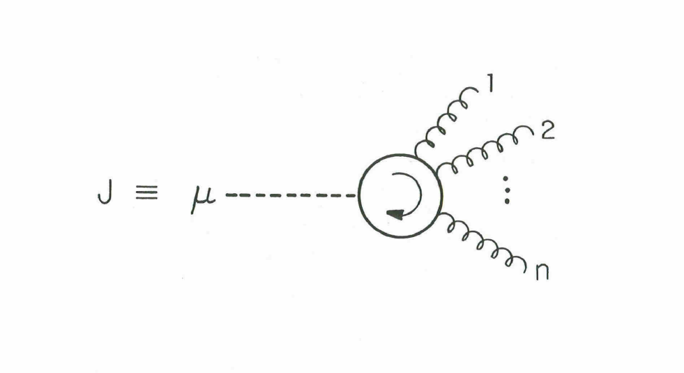
Figure 8: The color ordered gluonic current.

From the set of color truncated Feynman diagrams that make up the subamplitude, $m(1,2,\dots,n)$, one can form a color ordered gluonic current by replacing the polarization vector of the $n-th$ gluon with the propagator and allowing the momentum of this gluon to be off mass shell but still retain momentum conservation. This color ordered gluonic current will be represented by Fig. 8, where the dotted line represents the gluon which is off mass shell. This current will be written as $J_{\mu}(1,\dots,n-1)$ and the subamplitude can be reconstructed from this current by multiplying by the inverse propagator and contracting with a polarization vector and allowing the momentum of this gluon to be on mass shell,

$$\mbox{$m(1,2,\dots,n)$}~{}=\{\epsilon^{\mu}(p_{n})~{}i[P(1,n-1)]^{2}~{}\mbox{$J_{\mu}(1,\dots,n-1)$}\}~{}|_{P(1,n-1)=-p_{n}},$$ (7.1)

where, $P(1,n)\equiv\sum_{1}^{n}p_{i}$.

Of course these currents, $J_{\mu}$, are not gauge invariant and do depend on the choice of reference momenta chosen for the $(n-1)$ on mass shell gluons. Also they depend on the helicity of the on mass shell gluons. However these color ordered gluonic currents can be used as building blocks for gluonic currents with more external on mass shell legs.

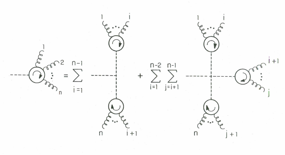
Figure 9: A graphical representation for the Berends-Giele gluonic recursion relation.

Consider a gluonic current with $n$ on mass shell gluons. Then the off mass shell gluon is attached to the rest of the gluons either through a three or a four point color ordered gluon coupling. At these vertices the other legs are attached to color ordered gluonic currents with fewer than $n$ on mass shell gluons. This can be seen diagrammatically in Fig. 9. Hence, the color ordered gluonic current with $n$ on mass shell gluons can be written in terms of gluonic currents with less than $n$ on mass shell gluons. This is the Berends-Giele recursion relation${}^{\cite[cite]{[\@@bibref{}{bg88}{}{}]}}$ for gluonic color ordered currents and algebraically it is written as

$$J_{\mu}(1,\dots,n) = {-i\over P(1,n)^{2}}\{\sum_{i=1}^{n-1}V3^{\mu\nu\rho}(P(1,i),P(i+1,n))~{}\mbox{$J_{\nu}(1,\dots,i)$}~{}\mbox{$J_{\rho}(i+1,\dots,n)$}$$ (7.2)

$$+~{}\sum_{j=i+1}^{n-1}~{}\sum_{i=1}^{n-2}V4^{\mu\nu\rho\sigma}~{}~{}\mbox{$J_{\nu}(1,\dots,i)$}~{}\mbox{$J_{\rho}(i+1,\dots,j)$}~{}\mbox{$J_{\sigma}(j+1,\dots,n)$}\}$$

where the color ordered three and four gluon vertices are, see Appendix C,

$$V3^{\mu\nu\rho}(P,Q) = i{g\over\sqrt{2}}~{}(g^{\nu\rho}~{}(P-Q)^{\mu}~{}+~{}2g^{\rho\mu}~{}Q^{\nu}~{}-~{}2g^{\mu\nu}~{}P^{\rho}),$$

$$V4^{\mu\nu\rho\sigma} = i{g^{2}\over 2}~{}(2g^{\mu\rho}~{}g^{\nu\sigma}~{}-~{}g^{\mu\nu}~{}g^{\rho\sigma}~{}-~{}g^{\mu\sigma}~{}g^{\nu\rho}).$$ (7.3)

The current with one on mass shell gluon is defined as

$$J_{\mu}(1)~{}\equiv~{}\epsilon_{\mu}(p_{1}).$$ (7.4)

The gluonic currents, $J_{\mu}(1,\dots,n)$, satisfy properties that are similar to the gluon subamplitude, $m(1,2,\dots,n)$.

1. Dual Ward identity:

   $$J_{\mu}(1,2,3,\dots,n)~{}+~{}J_{\mu}(2,1,3,\dots,n)\cdots~{}+~{}J_{\mu}(2,3,\dots,n,1)~{}=0.$$ (7.5)

2. Reflectivity:

   $$\mbox{$J_{\mu}(1,\dots,n)$}~{}=~{}(-1)^{n+1}~{}\mbox{$J_{\mu}(n,\dots,1)$}$$ (7.6)

3. $J_{\mu}(1,\dots,n)$ is conserved:

   $$P(1,n)^{\mu}~{}\mbox{$J_{\mu}(1,\dots,n)$}~{}=~{}0$$ (7.7)

There are simple analytical expressions for the color ordered gluonic currents if all the helicities are the same or if one is different from the others. Of course we must define the reference momentum for the gluons. Here the symbol $i$ for the gluons must be expanded to $i^{\lambda}_{k}$ where the $i$-th gluon has helicity $\lambda$ and reference light-like momentum $k$. Then

$$J_{\mu}(1^{+}_{k},2^{+}_{k},\dots,n^{+}_{k})~{}=~{}g^{n-1}{{\mbox{$\langle k-\!|\,$}~{}\gamma_{\mu}~{}\hat{P}(1,n)~{}\mbox{$\,|k+\rangle$}}\over{\sqrt{2}~{}\mbox{$\langle k1\rangle$}~{}\mbox{$\langle 12\rangle$}\cdots\mbox{$\langle n-1n\rangle$}~{}\mbox{$\langle nk\rangle$}}}$$ (7.8)

and

$$J_{\mu}(1^{-}_{k},2^{-}_{k},\dots,n^{-}_{k})~{}=~{}(-1)^{n}~{}g^{n-1}{{\mbox{$\langle k+\!|\,$}~{}\gamma_{\mu}~{}\hat{P}(1,n)~{}\mbox{$\,|k-\rangle$}}\over{\sqrt{2}~{}\mbox{$[k1]$}~{}\mbox{$[12]$}\cdots\mbox{$[n-1n]$}~{}\mbox{$[nk]$}}}.$$ (7.9)

Berends and Giele, ref.[12], give compact expressions for $J_{\mu}(1^{\mp},2^{\pm},\dots,n^{\pm})$ for a given choice of reference momenta. Also, Kosower, ref.[58], has given a light-cone formulation of these recursion relation to derive the sub-amplitudes $m(-,-,-,+,\cdots,+)$. Kleiss and Kuijf, Ref.[54], have used these recursion relations to calculate the 7-gluon amplitudes numerically.

7.2 Color Ordered Quark Currents

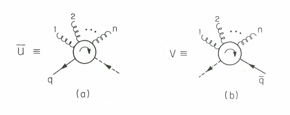
Figure 10: The quark, (a), and antiquark, (b), color ordered spinorial currents.

For the subamplitudes involving a quark-antiquark pair and gluons one can define a Quark and Antiquark color ordered spinorial current, see Fig. 10, in a way similar to the gluon currents that were defined in the last section. We will write the Quark current as $\overline{U}(q,1,\dots,n)$ and the Antiquark current as $V(1,\dots,n,\overline{q})$. The quark-antiquark pair plus gluon subamplitudes can be obtained from these currents as follows:

$$m(q,1,\dots,n,\overline{q}) =\mbox{$\langle q~{}\!|\,$}(+i)(\hat{\overline{q}}+\hat{P}(1,n))\mbox{$V(1,\dots,n,\overline{q})$}~{}|_{\overline{q}+P(1,n)=-q}$$ (7.10)

$$=\mbox{$\overline{U}(q,1,\dots,n)$}(-i)(\hat{q}+\hat{P}(1,n))\mbox{$\,|\overline{q}\rangle$}~{}|_{q+P(1,n)=-\overline{q}}$$

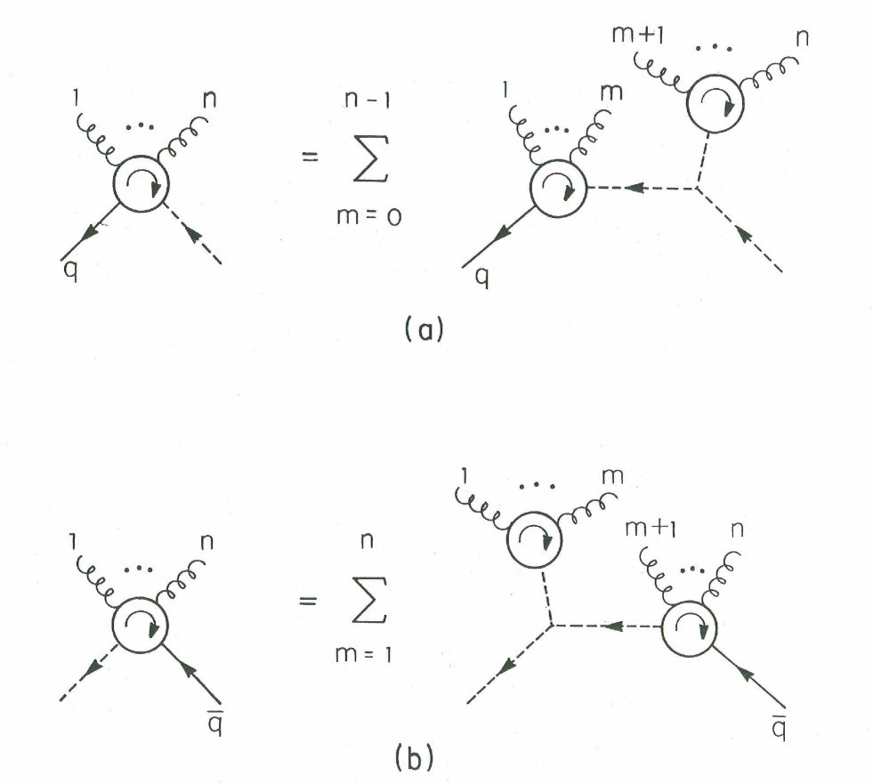
Figure 11: Graphical representations of the Berends-Giele quark, (a), and antiquark, (b), recursion relations.

In manner similar to the gluon current, a recursion relation can be written for this color ordered Quark current [12], see Fig. 11and Appendix C,

$$\mbox{$\overline{U}(q,1,\dots,n)$}~{}=~{}\sum_{m=0}^{n-1}\mbox{$\overline{U}(q,1,\dots,m)$}{ig\over\sqrt{2}}\gamma^{\mu}\mbox{$J_{\mu}(m+1,\dots,n)$}{i\over(\hat{q}~{}+~{}\hat{P}(1,n))}$$ (7.11)

and for the Anti-quark current${}^{\cite[cite]{[\@@bibref{}{bg88}{}{}]}}$

$$\mbox{$V(1,\dots,n,\overline{q})$}=\sum_{m=1}^{n}{-i\over(\hat{\overline{q}}+\hat{P}(1,n))}{ig\over\sqrt{2}}\gamma^{\mu}\mbox{$J_{\mu}(1,\dots,m)$}\mbox{$V(m+1,\dots,n,\overline{q})$}$$ (7.12)

and where the spinor currents for the zero gluon case are defined to be

$$\overline{U}(q)~{}\equiv~{}\overline{u}(q),\quad\quad\quad V(\overline{q})~{}\equiv~{}v(\overline{q})$$ (7.13)

in Bjorken and Drell notation.

These color ordered spinor currents can be defined for massive or massless quarks. For massive quarks the propagators in the recursion relations Eqs. (7.11,7.12) must be modified by adding the appropriate mass term. For massless quarks these spinor currents carry a chirality such that

$$(1~{}\pm~{}\gamma_{5})~{}\mbox{$V(1,\dots,n,\overline{q}^{\pm})$}~{}=0,\quad\quad\quad\mbox{$\overline{U}(q^{\pm},1,\dots,n)$}(1~{}\pm~{}\gamma_{5})~{}=0.$$ (7.14)

Also for the massless case the zero gluon currents are simply

$$\overline{U}(q^{\pm})~{}\equiv~{}\mbox{$\langle q\pm\!|\,$},\quad\quad\quad V(\overline{q}^{\pm})~{}\equiv~{}\mbox{$\,|\overline{q}\mp\rangle$}.$$ (7.15)

Again there are simple analytic expressions for these color ordered spinor currents when all the gluons have the same helicity as the fermion,

$$\mbox{$\overline{U}(q^{+},1^{+}_{k},\dots,n^{+}_{k})$}~{}=~{}-g^{n}~{}{\mbox{$\langle k-\!|\,$}(\hat{q}+\hat{P}(1,n))\over\mbox{$\langle q1\rangle$}\mbox{$\langle 12\rangle$}\cdots\mbox{$\langle nk\rangle$}},$$ (7.16)

$$\mbox{$\overline{U}(q^{-},1^{-}_{k},\dots,n^{-}_{k})$}~{}=~{}-(-g)^{n}~{}{\mbox{$\langle k+\!|\,$}(\hat{q}+\hat{P}(1,n))\over\mbox{$[q1]$}\mbox{$[12]$}\cdots\mbox{$[nk]$}},$$ (7.17)

$$\mbox{$V(1^{+}_{k},\dots,n^{+}_{k},\overline{q}^{+})$}~{}=~{}-g^{n}~{}{(\hat{\overline{q}}+\hat{P}(1,n))\mbox{$\,|k+\rangle$}\over\mbox{$\langle k1\rangle$}\mbox{$\langle 12\rangle$}\cdots\mbox{$\langle n\overline{q}\rangle$}},$$ (7.18)

and

$$\mbox{$V(1^{-}_{k},\dots,n^{-}_{k},\overline{q}^{-})$}~{}=~{}-(-g)^{n}~{}{(\hat{\overline{q}}+\hat{P}(1,n))\mbox{$\,|k-\rangle$}\over\mbox{$[k1]$}\mbox{$[12]$}\cdots\mbox{$[n\overline{q}]$}}.$$ (7.19)

If there is one gluon with opposite helicity to that of the fermion, the spinorial currents are

$$\overline{U}(q^{+},1^{-}_{k})~{}=~{}-g~{}{{\mbox{$[qk]$}\mbox{$\langle q+\!|\,$}}\over{\mbox{$[q1]$}\mbox{$[1k]$}}},$$ (7.20)

$$\overline{U}(q^{-},1^{+}_{k})~{}=~{}g~{}{{\mbox{$\langle qk\rangle$}\mbox{$\langle q-\!|\,$}}\over{\mbox{$\langle q1\rangle$}\mbox{$\langle 1k\rangle$}}},$$ (7.21)

$$V(1^{-}_{k},\overline{q}^{+})~{}=~{}-g~{}{{\mbox{$\,|\overline{q}-\rangle$}\mbox{$[k\overline{q}]$}}\over{\mbox{$[k1]$}\mbox{$[1\overline{q}]$}}}$$ (7.22)

and

$$V(1^{+}_{k},\overline{q}^{-})~{}=~{}g~{}{{\mbox{$\,|\overline{q}+\rangle$}\mbox{$\langle k\overline{q}\rangle$}}\over{\mbox{$\langle k1\rangle$}\mbox{$\langle 1\overline{q}\rangle$}}}.$$ (7.23)

Finally, for two gluons with opposite helicity, we have the following spinorial currents,

$$\overline{U}(q^{-},1^{+}_{2},2^{-}_{1})~{}=~{}{-g^{2}~{}\mbox{$\langle q2\rangle$}^{2}\over\mbox{$\langle q1\rangle$}S_{12}(q+1+2)^{2}}\mbox{$\langle 1+\!|\,$}(\hat{q}+\hat{1}+\hat{2}),$$ (7.24)

$$\overline{U}(q^{-},1^{-}_{2},2^{+}_{1})~{}=~{}{g^{2}~{}\mbox{$[2q]$}\mbox{$\langle q1\rangle$}\over\mbox{$[q1]$}S_{12}(q+1+2)^{2}}\mbox{$\langle 2+\!|\,$}(\hat{q}+\hat{1}+\hat{2}),$$ (7.25)

$$V(1^{+}_{2},2^{-}_{1},\overline{q}^{+})~{}=~{}(\hat{1}+\hat{2}+\hat{\overline{q}})\mbox{$\,|2+\rangle$}{-g^{2}~{}\mbox{$[1\overline{q}]$}^{2}\over(1+2+\overline{q})^{2}S_{12}\mbox{$[2\overline{q}]$}}$$ (7.26)

and

$$V(1^{-}_{2},2^{+}_{1},\overline{q}^{+})~{}=~{}(\hat{1}+\hat{2}+\hat{\overline{q}})\mbox{$\,|1+\rangle$}{g^{2}~{}\mbox{$[2\overline{q}]$}\mbox{$\langle\overline{q}1\rangle$}\over(1+2+\overline{q})^{2}S_{12}\mbox{$\langle 2\overline{q}\rangle$}}.$$ (7.27)

A straight forward example using these currents is to calculate the sub-amplitude for $(q^{-},1^{+},2^{-},\overline{q}^{+})$ process,

$$m(q^{-},1^{+},2^{-},\overline{q}^{+}) = \overline{U}(q^{-})~{}i(\hat{1}+\hat{2}+\hat{\overline{q}})~{}V(1^{+}_{2},2^{-}_{1},\overline{q}^{+})$$ (7.28)

$$= {ig^{2}~{}\mbox{$\langle q2\rangle$}^{3}\mbox{$\langle\overline{q}2\rangle$}\over\mbox{$\langle q1\rangle$}\mbox{$\langle 12\rangle$}\mbox{$\langle 2\overline{q}\rangle$}\mbox{$\langle\overline{q}q\rangle$}},$$

which is the previously obtained result. The spinorial currents defined here can be used to derive many of the results of other section, especially the section involving multiple gauge groups.

8 Exact Results for n-Parton Amplitudes

The interest in exact matrix elements for $n$-parton processes in QCD was started in 1986 by Parke and Taylor [81] who realized that certain non-trivial helicity amplitudes in pure Yang-Mills theory could be written in a simple closed form. These same helicity amplitudes have been extended to processes including quarks,in Ref.[68, 69], and Vector Bosons, in Ref.[12, 65], and are also used as the starting point for approximation schemes, in Ref.[62, 74], for processes involving a large number of partons. These Generalized Parke and Taylor amplitudes are the subject of this section.

The Berends and Giele recursive relations presented in the previous Section are an extremely powerful tool to derive expressions for processes with a large number of partons. They have been used up to now to obtain the amplitudes for 7- and 8-gluon processes [16, 17] and for processes with a color-singlet vector boson and up to 5 colored partons [15], in this case confirming the results independently obtained by Hagiwara and Zeppenfeld in Ref.[48]. Unfortunately most of the resulting formulae are very complex and hard to interpret. It is very interesting, however, that for some special helicity configurations the matrix elements conserve a very simple universal structure independently of the number of particles involved.

In this Section we present a collection of exact results which hold for a specific set of helicity amplitudes with an arbitrary number of particles. The interest in these expressions is not just academic, as these results can be used as the starting point for the development of very powerful approximation techniques that will be described in a following Section. Furthermore they help clarifying the dynamical features of hard multi-particle processes and shed additional light on the structure of quantum coherence in the radiation of abelian and non-abelian radiation, as we will discuss.

8.1 Helicity Violating Amplitudes

Let us consider processes with the following helicity structure:

$$(-,-,+\dots,+)\quad\mbox{or}\quad(+,+,-,\dots,-).$$ (8.1)

We will call these helicity structures Maximally Helicity Violating (MHV) . It is straightforward to prove that the only singularities the corresponding amplitudes may have are soft and collinear poles of the form $1/\sqrt{(}p_{i}\cdot p_{j})$. Because of factorization, the residues at these poles are fixed, and given by the product of a proper Altarelli-Parisi splitting function times an $(n-1)$-parton MHV amplitude:

$$m^{(n)}(-,-,+\dots,+)\rightarrow{1\over\sqrt{(}p_{i}p_{j})}\sqrt{f(z)}m^{(n-1)}(-,-,+\dots,+).$$ (8.2)

The A-P function that will appear depends on the helicities of the collinear partons.

As an example, we can take the 5-gluon amplitude, Eq. (5.16):

$$m(g_{1}^{-},g_{2}^{-},g_{3}^{+},g_{4}^{+},g_{5}^{+})\;=\;i\,\mbox{$g_{s}^{3}$}\,{\mbox{$\langle 12\rangle$}^{4}\over\mbox{$\langle 12\rangle$}\mbox{$\langle 23\rangle$}\mbox{$\langle 34\rangle$}\mbox{$\langle 45\rangle$}\mbox{$\langle 51\rangle$}}.$$ (8.3)

If we study the behaviour of this sub-amplitude near the three inequivalent poles $s_{23}\rightarrow 0$, $s_{45}\rightarrow 0$ and $s_{51}\rightarrow 0$, we obtain the following factorization relations:

$$m^{(5)} \rightarrow {1\over\mbox{$\langle 23\rangle$}}\;g\;\sqrt{{z^{4}\over z(1-z)}}~{}ig^{2}~{}{\mbox{$\langle 1P\rangle$}^{4}\over\mbox{$\langle 1P\rangle$}\mbox{$\langle P4\rangle$}\mbox{$\langle 45\rangle$}\mbox{$\langle 51\rangle$}},$$ (8.4)

$$m^{(5)} \rightarrow {1\over\mbox{$\langle 45\rangle$}}\;g\;\sqrt{{1\over z(1-z)}}~{}ig^{2}~{}{\mbox{$\langle 12\rangle$}^{4}\over\mbox{$\langle 12\rangle$}\mbox{$\langle 23\rangle$}\mbox{$\langle 3P\rangle$}\mbox{$\langle P1\rangle$}},$$ (8.5)

$$m^{(5)} \rightarrow {1\over\mbox{$\langle 51\rangle$}}\;g\;\sqrt{{(1-z)^{4}\over z(1-z)}}~{}ig^{2}~{}{\mbox{$\langle P2\rangle$}^{4}\over\mbox{$\langle P2\rangle$}\mbox{$\langle 23\rangle$}\mbox{$\langle 34\rangle$}\mbox{$\langle 4P\rangle$}},$$ (8.6)

with :

$$i\;=\;zP+{\cal O}(\sqrt{(i\cdot j)}),\quad j\;=\;(1-z)P+{\cal O}(\sqrt{(i\cdot j)}),$$ (8.7)

$i$ and $j$ being the two collinear momenta. As expected, the first terms on the right-hand side of Equations (8.4)-(8.6) are the four-gluon sub-amplitudes, Equation (5.5), and the second terms are the square roots of the polarized A-P functions.

Lorentz invariance and the factorization properties uniquely fix the form of the amplitudes at tree level (their squares are just rational functions), and for the MHV amplitudes these constraints can be easily solved explicitly with simple ’educated guesses’ of what the amplitude might be. More formally, these amplitudes can be derived by solving the Berends and Giele recursive relations, which for these helicity configurations turn out to be particularly simple [12, 67].

For purely gluonic processes, the MHV amplitudes are given by the obvious generalizations of Equations (5.5) and (5.16) :

$$M(g^{-}_{1},g^{-}_{2},g^{+}_{3},\dots,g^{+}_{n})=ig^{n-2}\langle 12\rangle^{4}\sum_{\{1,2,\dots\}^{\prime}}\;tr(\lambda_{1}\lambda_{2}\cdots\lambda_{n}){1\over\langle 12\rangle\langle 23\rangle\cdots\langle n1\rangle},$$ (8.8)

where the sum is taken over the $(n-1)!$ non-cyclic permutations of the indices. It is easy to show that this Equation satisfies all the required factorization properties and the Dual Ward Identities.

At the leading order in $N^{\ }$the square of these gluonic matrix elements, summed over colors, and over all the MHV configurations, gives the so called Parke and Taylor Amplitudes [81]:

$$|M(g_{1},\dots,g_{n})|^{2}\;=\;2\mbox{$g_{s}^{2n-4}$}\mbox{$N^{n-2}$}(\mbox{$N^{2}$}-1)\sum_{i>j}s_{ij}^{4}\;\sum_{\{1,2,\dots,n\}^{\prime}}\;{1\over s_{12}s_{23}s_{34}\dots s_{n1}}.$$ (8.9)

The overall factor of 2, coming from the sum over $(--++\dots+)$ and $(++--\dots-)$ configurations, is clearly absent for $n=4$

Recently a universal form was found [58] also for a specific set of gluonic non-MHV sub-amplitudes, namely for helicity configurations of the following form and in the indicated order: $(---+++\dots+)$. This form is not as simple as the Parke and Taylor expression, therefore we will not display it here and we refer to the original paper for the explicit result.

By using the Supersymmetry Ward Identity given in Equation (4.9) we can now derive the MHV amplitudes for processes with a pair of (massless) gluinos or a $q\bar{q}$ pair:

$$M(g^{-}_{1},\Lambda^{-}_{2},\Lambda^{+}_{3},g^{+}_{4},\dots,g^{+}_{n})=ig^{n-2}\langle 12\rangle^{3}\langle 13\rangle\sum_{\{1,2,\dots,n\}^{\prime}}\;tr(\lambda_{1}\lambda_{2}\cdots\lambda_{n}){1\over\langle 12\rangle\langle 23\rangle\cdots\langle n1\rangle},$$

(8.10)

$$M(q^{-},g^{-}_{1},g^{+}_{2},\dots,g^{+}_{n},\bar{q}^{+})=ig^{n}{\langle q1\rangle^{3}\langle\bar{q}1\rangle\over\mbox{$\langle\bar{q}q\rangle$}}\sum_{\{1,2,\dots,n\}}\;(\lambda_{1}\lambda_{2}\cdots\lambda_{n})_{ij}{1\over\langle q1\rangle\langle 12\rangle\cdots\langle n\bar{q}\rangle}.$$

(8.11)

We can once again square these matrix elements at the leading order in $N$, and obtain:

$$|M(g_{1},\Lambda_{2},\Lambda_{3},g_{4},\dots,g_{n})|^{2}\;=\; 2\mbox{$g_{s}^{2n-4}$}\mbox{$N^{n-2}$}(\mbox{$N^{2}$}-1)\sum_{i\neq 2,3}(s_{2i}^{3}s_{3i}+s_{2i}s_{3i}^{3})\;$$ (8.12)

$$\times\sum_{\{1,2,\dots,n\}^{\prime}}\;{1\over s_{12}s_{23}s_{34}\dots s_{n1}},$$

$$|M(q,g_{1},\dots,g_{n},\bar{q})|^{2}\;=\; 2\mbox{$g_{s}^{2n}$}\mbox{$N^{n-1}$}(\mbox{$N^{2}$}-1)\sum_{i=1}^{n}(s_{qi}^{3}s_{\bar{q}i}+s_{qi}s_{\bar{q}i}^{3})\;$$ (8.13)

$$\times{1\over s_{q\bar{q}}}\sum_{\{1,2,\dots,n\}}\;{1\over s_{q1}s_{12}\dots s_{n\bar{q}}}.$$

Even though massless supersymmetric particles do not exist, the $m=0$ approximation might turn out to be useful if they were discovered to be relatively light on the scale of the future hadronic supercolliders, where their properties would be studied in detail.

Let us now take the amplitude $M(\Lambda^{+}_{1},\Lambda^{-}_{2},\Lambda^{+}_{3},g^{-}_{4},g^{+}_{5},\dots,g^{+}_{n})$. By commuting with the supersymmetry operator and properly choosing the reference momentum $k$ we obtain the following SWI:

$$M_{\tilde{g}}(\Lambda^{+}_{1},\Lambda^{+}_{2},\Lambda^{-}_{3},\Lambda^{-}_{4},g^{+}_{5},\dots,g^{+}_{n})={\langle 12\rangle\over\langle 24\rangle}M_{\tilde{g}}(g^{+}_{1},\Lambda^{+}_{2},\Lambda^{-}_{3},g^{-}_{4},g^{+}_{5},\dots,g^{+}_{n}).$$ (8.14)

By using Equation (8.10) we get:

$$M_{\tilde{g}}(\Lambda^{+}_{1},\Lambda^{+}_{2},\Lambda^{-}_{3},\Lambda^{-}_{4},g^{+}_{5},\dots,g^{+}_{n})=ig^{n-2}\langle 12\rangle\langle 34\rangle^{3}\sum_{perm^{\prime}}\;tr(\lambda_{1}\lambda_{2}\cdots\lambda_{n}){1\over\langle 12\rangle\langle 23\rangle\cdots\langle n1\rangle}.$$ (8.15)

The MHV amplitude for the scattering of gluons and a pair of massless scalar-quarks is obtained from the SWI and the supersymmetry transformations of a chiral superfield${}^{\cite[cite]{[\@@bibref{}{susy1,susy2}{}{}]}}$:

$$M(\bar{\phi}^{+}_{1},\phi^{-}_{2},g^{-}_{3},g^{+}_{4},\dots,g^{+}_{n})=ig^{n-2}\langle 23\rangle^{2}\langle 13\rangle^{2}\sum_{\{3,\dots,n\}}\;(\lambda_{3}\lambda_{4}\cdots\lambda_{n})_{i_{2}i_{1}}\;{1\over\langle 12\rangle\langle 23\rangle\cdots\langle n1\rangle}.$$ (8.16)

$\phi^{\pm}$ are the supersymmetry partners of the two helicity states of the quark. The two combinations $\phi^{+}\pm\phi^{-}$ transform respectively as a scalar and a pseudoscalar under the Lorentz group. For $n=4,5$ these are the only independent non-vanishing helicity amplitudes for this process.

It is interesting to notice, even though the authors do not have a clear understanding of the deep reasons for this result, that all of these exact matrix elements for the MHV amplitudes with gluons, fermions and scalars can be generated in a straightforward way as correlation functions of fields of a two-dimensional Wess-Zumino-Witten gauge model with $N=4$ supersymmetry [77].

8.2 Color Coherence

Let us go back now to the $q\bar{q}$ plus gluons process, Equation (8.11): if we put the color factors $(\lambda^{a_{1}}\dots\lambda^{a_{n}})_{ij}$ equal to 1 for each permutation of 1 through $n$, then Equation (8.11) gives rise to the QED result for the amplitude with one quark-pair and $n$ photons. This can be easily proved diagrammatically by observing that diagrams with non-abelian gluon vertices entering the graph expansion for the sub-amplitudes cancel in pairs when we perform the sum over permutations. In this way the only diagrams left are the QED-type diagrams, with the common trivial abelian color structure. This result is independent of the helicity configuration, and for the helicities considered above we then obtain:

$$M^{n}_{\gamma}(h_{q},h_{\gamma})=i\,(\sqrt{2}e)^{n}{\{p\gamma\}^{3}\{\mbox{$\bar{p}$}\gamma\}\over\{p\mbox{$\bar{p}$}\}}\,\sum_{\{1,2,\dots,n\}}{1\over\{p1\}\{12\}\dots\{n\mbox{$\bar{p}$}\}},$$ (8.17)

where $\gamma$ is the momentum of the photon with helicity different from the others, $h_{\gamma}$ is its helicity, and where the curly brackets stand for the spinor products or their complex conjugates, depending on the helicity of the photon:

$$\{ij\}_{h_{\gamma}=-}=\langle ij\rangle\quad,\quad\{ij\}_{h_{\gamma}=+}=[ij]$$ (8.18)

The following remarkable identity holds:

$$\sum_{\{1,2,\dots,n\}}{\{p\mbox{$\bar{p}$}\}\over\{p1\}\{12\}\dots\{n\mbox{$\bar{p}$}\}}\;=\;\prod_{i=1}^{n}\;{\{p\mbox{$\bar{p}$}\}\over\{pi\}\{i\mbox{$\bar{p}$}\}}.$$ (8.19)

Equation (8.19) can be proved by iteratively using the Fierz identity:

$$\{p\mbox{$\bar{p}$}\}\{q\bar{q}\}\;=\;\{p\bar{q}\}\{q\mbox{$\bar{p}$}\}+\{pq\}\{\mbox{$\bar{p}$}\bar{q}\}.$$ (8.20)

Equation (8.19) can be thought of as a sort of ‘square root’ of the eikonal identity. It allows us to put equation (8.17) into the eikonalized form:

$$M^{n}_{\gamma}(h_{q},h_{\gamma})=i\,(\sqrt{2}e)^{n}\delta_{ij}{\{p\gamma\}^{3}\{\mbox{$\bar{p}$}\gamma\}\over\{p\mbox{$\bar{p}$}\}^{2}}\,\prod_{i=1}^{n}\;{\{p\mbox{$\bar{p}$}\}\over\{pi\}\{i\mbox{$\bar{p}$}\}}.$$ (8.21)

Equations (8.11), (8.17) and (8.21) offer a nice example of the difference between the properties of the non-abelian radiation as opposed to the abelian radiation. Let us take, in fact, the square of these three expressions, summed over the colors of the quarks and of the gluons (when present):

$$\sum_{col}|M^{n}(h_{q},h_{g})|^{2}=g^{2n}N^{n+1}{(pg)^{3}(\mbox{$\bar{p}$}g)\over(p\mbox{$\bar{p}$})}\,\sum_{\{1,2,\dots,n\}}{1\over(p1)(12)\dots(n\mbox{$\bar{p}$})}\;+\;{1\over N^{2}}(interf.),$$

(8.22)

$$\sum_{col}|M^{(n)}_{\gamma}(h_{q},h_{\gamma})|^{2}=(\sqrt{2}e)^{2n}N{(p\gamma)^{3}(\mbox{$\bar{p}$}\gamma)\over(p\mbox{$\bar{p}$})}\,\sum_{\{1,2,\dots,n\}}{1\over(p1)(12)\dots(n\mbox{$\bar{p}$})}\;+\;(interf.),$$

(8.23)

$$\sum_{col}|M^{(n)}_{\gamma}(h_{q},h_{\gamma})|^{2}=(\sqrt{2}e)^{2n}N{(p\gamma)^{3}(\mbox{$\bar{p}$}\gamma)\over(p\mbox{$\bar{p}$})^{2}}\,\prod_{i=1}^{n}{(p\mbox{$\bar{p}$})\over(pi)(i\mbox{$\bar{p}$})},$$ (8.24)

where:

$$(ij)=2\;i\cdot j.$$ (8.25)

Equations (8.23) and (8.24) are identical, thanks to the eikonal identity, but we wrote them in the two different ways to establish a connection with the expression for the gluon emission. Equation(8.24) shows that the photon emission is incoherent: the photons only know about their source, i.e. the quark line, but they do not know about each other. Up to the overall factor in front, the probability for the emission of $n$ photons is just the product of the probabilities for the independent emission of each of them.

On the contrary, if we now look at equation (8.22) we see that the gluon emission is not incoherent: gluons know of each other’s presence, and the full probability is not a product of probabilities. The interference terms coming from the product of different permutations are suppressed by a factor of $1/N^{2}$; this suppression originates from the interferences of the color factors. For the photon emission, vice versa, we can see from equation (8.23) that the interferences among different permutations are not suppressed and they conspire to cancel the coherence apparent into the sum of squares, giving rise to the factorized expression given in (8.24).

The phenomenological consequences of this coherence effects have been explored experimentally [52] (the string effect) and theoretically (see for example [7, 4, 10, 71, 34, 29, 72]).

8.3 $q\bar{q}q\bar{q}$ plus gluons

In general the factorization of the color structure exhibited in equation (3.9) does not imply a similar factorization of the kinematical part of the amplitude. In other words, the sub-amplitude that multiplies a given color factor does not factorize into products of terms that only depend upon the kinematical variables (helicities and momenta) of the particles belonging to the same antenna. One remarkable non-trivial exception to this general feature is given by the amplitude for a process with two quark pairs and an arbitrary number of like-helicity gluons (all the particles are outgoing). Up to an overall factor that only depends upon the helicity configuration each sub-amplitude factorizes into the product of two terms that only depend upon the momenta of the gluons emitted by one or the other of the two antennas:

$$M(h_{p},h_{q},h_{g}) =\;i\,g^{n+2}A_{0}(h_{p},h_{q},h_{g})\;\;\cdot$$

$$\sum {\{p\bar{q}\}\over\{pa_{1}\}\{a_{1}a_{2}\}\cdots\{a_{k}\bar{q}\}}{\{q\bar{p}\}\over\{qb_{1}\}\{b_{1}b_{2}\}\cdots\{b_{k^{\prime}}\bar{p}\}}(\lambda^{a_{1}}\cdots\lambda^{a_{k}})_{i_{1}j_{2}}(\lambda^{b_{1}}\cdots\lambda^{b_{k^{\prime}}})_{i_{2}j_{1}}$$

$$-{1\over N} {\{p\bar{p}\}\over\{pa_{1}\}\{a_{1}a_{2}\}\cdots\{a_{k}\bar{p}\}}{\{q\bar{q}\}\over\{qb_{1}\}\{b_{1}b_{2}\}\cdots\{b_{k^{\prime}}\bar{q}\}}(\lambda^{a_{1}}\cdots\lambda^{a_{k}})_{i_{1}j_{1}}(\lambda^{b_{1}}\cdots\lambda^{b_{k^{\prime}}})_{i_{2}j_{2}}.$$

The helicity structure of this amplitude uniquely determines the pole structure and the residues of these poles, through unitarity: Equation(8.3) is the only Lorentz invariant amplitude that gives rise to the right poles and the right residues. Alternatively, one can prove Equation (8.3) by using the appropriate form of the Berends and Giele recursive relations [12].

If the gluons have all positive helicity, then $\{ij\}=\mbox{$\langle ij\rangle$}$, otherwise $\{ij\}=\mbox{$[ij]$}$. The indices $p$ and $q$ ($\bar{p}$ and $\bar{q}$) refer to the quarks (antiquarks) and the indices $a_{\alpha},b_{\beta}$ refer to the gluons. The arguments $h$ represent the helicities of the two quarks and of the gluons; the helicities of the anti-quarks are fixed by helicity conservation along the fermion lines. The sum is over all the partitions of the $n$ gluons ($k+k^{\prime}=n,k=0,1,\dots,n$) and over the permutations of the gluon indices. When $k=(0,n)$ the product of zero $\lambda$ matrices becomes a Kronecker delta and one of the two kinematical factors is equal to one. The overall factor $A_{0}$ can be written as follows:

$$A_{0}(h_{p},h_{q},h_{g})\;=\;{a_{0}(h_{p},h_{q},h_{g})\over(p+\mbox{$\bar{p}$})^{2}(q+\bar{q})^{2}}.$$ (8.27)

The functions $a_{0}$ are given in Table 5, where helicity configurations obtained by permuting the quark helicities have been omitted. The functions $a_{0}$ are universal, in the sense that they only depend upon the spin-1/2 nature of the quarks. As we will see later, they also enter in processes like deep inelastic scattering or $e^{+}e^{-}$ annihilation.

$(h_{p},h_{q},h_{g})$	$a_{0}(h_{p},h_{q},h_{g})$
$(+,+,+)$	$\langle\mbox{$\bar{p}$}\bar{q}\rangle^{2}[p\mbox{$\bar{p}$}][q\bar{q}]$
$(+,+,-)$	$[pq]^{2}\langle p\mbox{$\bar{p}$}\rangle\langle q\bar{q}\rangle$
$(+,-,+)$	$\langle\mbox{$\bar{p}$}q\rangle^{2}[p\mbox{$\bar{p}$}][q\bar{q}]$
$(+,-,-)$	$[p\bar{q}]^{2}\langle p\mbox{$\bar{p}$}\rangle\langle q\bar{q}\rangle$

Table 5: The universal functions $a_{0}(h_{p},h_{q},h_{g})$.

To the leading order in $N$, the amplitude squared summed over colors is furthermore given by:

$$\sum_{col}|M(h_{p},h_{q},h_{g})|^{2} = g^{2n+4}N^{n}(N^{2}-1)|A_{0}(h_{p},h_{q},h_{g})|^{2}$$ (8.28)

$$\sum {(p\bar{q})\over(pa_{1})(a_{1}a_{2})\cdots(a_{k}\bar{q})}\,{(q\bar{p})\over(qb_{1})(b_{1}b_{2})\cdots(b_{k^{\prime}}\bar{p})}.$$

If the quarks are identical we must add the contribution from the crossed channel $p\leftrightarrow q$.

As in the case with one quark pair, we can here compare the properties of photon radiation with those of gluon radiation. A reasoning similar to the one used in the previous section allows us to write the amplitude for the emission of $n$ like-helicity photons off two quark-pairs:

$$M(h_{p},h_{q},h_{g}) = i\,g^{2}(\sqrt{2}e)^{n}A_{0}(h_{p},h_{q},h_{g})\;\;\cdot$$

$$\sum \!\!\!\!{\{p\bar{p}\}\over\{pa_{1}\}\{a_{1}a_{2}\}\cdots\{a_{k}\bar{p}\}}{\{q\bar{q}\}\over\{qb_{1}\}\{b_{1}b_{2}\}\cdots\{b_{k^{\prime}}\bar{q}\}}(\delta_{i_{1}j_{2}}\delta_{i_{2}j_{1}}-{1\over N}\delta_{i_{1}j_{1}}\delta_{i_{2}j_{2}}).$$

Only the contribution from gluon exchange is shown. The effect of photon exchange between the two quark-pairs can be easily added. A repeated use of the Fierz identity, equation (8.20), leads then to the following form of equation (LABEL:two_pair_ph):

$$M(h_{p},h_{q},h_{g}) = i\,g^{2}(\sqrt{2}e)^{n}A_{0}(h_{p},h_{q},h_{g})\;\;\cdot$$ (8.30)

$$\prod_{i=1}^{n} ({\{p\bar{p}\}\over\{pi\}\{i\bar{p}\}}+{\{q\bar{q}\}\over\{qi\}\{i\bar{q}\}})(\delta_{i_{1}j_{2}}\delta_{i_{2}j_{1}}-{1\over N}\delta_{i_{1}j_{1}}\delta_{i_{2}j_{2}}).$$

This expression shows that photons are emitted independently. Once again we expect this result to hold for an arbitrary helicity configuration in the soft-photon limit.

If we substitute the color factor in equation(8.30) with the Abelian one, $\delta_{i_{1}j_{1}}\delta_{i_{2}j_{2}}$, and if we put $g$=$\sqrt{2}e$, then we obtain the amplitude for the process $e^{+}e^{-}\mu^{+}\mu^{-}\ photons$, as given in reference [20, 93].

8.4 $e^{+}e^{-}$ and DIS

It is easy to derive expressions analogous to (8.3) and (8.28) for the process $l\bar{l}q\bar{q}\ gluons$, where $l\bar{l}$ is a lepton-antilepton pair (for example $e^{+}e^{-}$ or $e^{-}\bar{\nu}$) [12, 65]. Again the gluons have all the same helicity:

$$M^{l}(h_{l},h_{q},h_{g})\;=\;i\,g^{n}\sum_{V=\gamma,Z,W}M^{l}_{V}(h_{l},h_{q},h_{g})\,\sum_{\{1,2,\dots,n\}}(\lambda^{a_{1}}\dots\lambda^{a_{n}})_{ij}\,{\{q\bar{q}\}\over\{q1\}\{12\}\dots\{n\bar{q}\}},$$ (8.31)

$$\sum_{col}|M^{l}(h_{l},h_{q},h_{g})|^{2}\;=\;g^{2n}N^{n-1}(N^{2}-1)\;|\sum_{V=\gamma,Z,W}M^{l}_{V}(h_{l},h_{q},h_{g})|^{2}\,\sum_{\{1,\dots,n\}}{(q\bar{q})\over(q1)(12)\dots(n\bar{q})}.$$ (8.32)

$q$ and $\bar{q}$ are the quark momenta and 1 through $n$ are the gluon momenta. The contributions from photon,$W$ and $Z$ exchange are explicitly exhibited. The functions $M^{l}_{V}(h_{l},h_{q},h_{g})$ are given by:

$$M_{V}(h_{l},h_{q},h_{g})={Q_{V}(h_{l})Q_{V}(h_{q})\over(q+\bar{q})^{2}(s-M^{2}_{V})}\,a_{0}(h_{l},h_{q},h_{g})$$ (8.33)

$Q_{V}(h_{l})$  ($Q_{V}(h_{q})$) is the charge corresponding to the interaction of a lepton (quark) of helicity $h_{l}$ ($h_{q}$) with the vector $V$.  Furthermore $s=(p+\mbox{$\bar{p}$})^{2}$, with $p$ and $\bar{p}$ being the lepton momenta, and $M_{V}^{2}$ is the mass squared of the vector boson $V$. The universal functions $a_{0}(h_{l},h_{q},h_{g})$ coincide with those given in Table 5.

For $e^{+}e^{-}$ scattering the effect of photon radiation (both from the initial and the final state) can be easily incorporated into equation (8.31) by using equation (8.30). Here we will display directly the result for the square of the amplitude with $n$ gluons and $m$ photons, to the leading order in $N$:

$$\sum_{col}|M^{e^{+}e^{-}}(h_{l},h_{q},h_{g})|^{2}\;=\;(2e^{2})^{m}g^{2n}N^{n-1}(N^{2}-1)\;|\sum_{V=\gamma,Z}M^{l}_{V}(h_{l},h_{q},h_{g})|^{2}\times$$

$$\prod_{i=1}^{m}|({\{p\bar{p}\}\over\{pk_{i}\}\{k_{i}\bar{p}\}}+{\{q\bar{q}\}\over\{qk_{i}\}\{k_{i}\bar{q}\}})|^{2}\sum_{\{1,2,\dots,n\}}{(q\bar{q})\over(q1)(12)\dots(n\bar{q})}.$$ (8.34)

The $k_{i}$’s are the momenta of the photons. Once again this result is only exact if all the gluons and the photons have the same helicity, but this is the behaviour of all the other helicity configurations in the case of soft emission.

Exact expressions for the full calculation of the processes $e^{+}e^{-}\rightarrow 4$ partons were given in [31] (for the complete $O(\alpha^{2})$ calculation) and in [2] (tree level) and for the processes $e^{+}e^{-}\rightarrow 5$ partons in [48, 15] (tree level).

9 Multiple Gauge Groups

In a theory in which the fermions are coupled to a direct product gauge group, say $SU(M)\times SU(N)$, then the techniques described earlier in this report can also be implemented. In fact the subamplitudes can be easily obtained from the subamplitudes given earlier by adding various combinations of ‘color’ orderings together. This can also be extended to $U(1)$ gauge groups, e.g. electromagnetism. For spontaneously broken gauge groups, only processes involving a single vector boson are easily obtained from previous calculations. In this section we have set all coupling constants to unity, but the reader can easily insert the appropriate couplings.

9.1 $SU(M)\times SU(N)$

Consider a fermion which is in the fundamental representation of both $SU(M)$ and $SU(N)$, then the amplitude for scattering of a fermion-antifermion with $m$ vectors from $SU(M)$ and $\bar{n}$ vectors of $SU(N)$ can be written as

$$M(q,1,2,\dots,m;\bar{1},\bar{2},\dots,\bar{n},\overline{q}) = \sum_{P,\overline{P}}~{}~{}(\Lambda^{1}\Lambda^{2}\dots\Lambda^{m})_{i~{}j}~{}~{}(\lambda^{\bar{1}}\lambda^{\bar{2}}\dots\lambda^{\bar{n}})_{\bar{i}~{}\bar{j}}~{}~{}~{}~{}~{}~{}~{}~{}~{}$$ (9.1)

$$m_{M,N}(q,1,2,\dots,m,\overline{q};~{}q,\bar{1},\bar{2},\dots,\bar{n},\overline{q}).$$

$\Lambda$ and $\lambda$ are the fundamental matrices of $SU(M)$ and $SU(N)$ respectively. Also $ij$ and $\bar{i}\bar{j}$ are the $SU(M)$ and $SU(N)$ ‘color’ indices of the fermions and the sum is over all permutations of $1,2,\dots,m$ and $\bar{1},\bar{2},\dots,\bar{n}$.

The subamplitudes defined by Eq. (9.1) can be easily obtained from the subamplitudes obtained earlier, Eq. (4.10),

$$m_{M,N}(q,1,2,\dots,m,\overline{q};~{}q,\bar{1},\bar{2},\dots,\bar{n},\overline{q})~{}=~{}\sum_{I}m(q,1,2,\dots,m,\bar{1},\bar{2},\dots,\bar{n},\overline{q})$$ (9.2)

where the $\sum_{I}$ is over all ways the barred numbers can be interspersed within the unbarred numbers maintaining the order of both the barred and unbarred numbers. This sum causes all Feynman diagrams which connect directly the vectors of $SU(M)$ with $SU(N)$ to be cancelled.

As an example, consider the scattering in which the fermion has negative helicity and the $\alpha$ vector boson of either gauge group has negative helicity and all particles have positive helicity. Then,

$$m_{M,N}(q,1,\dots,m,\overline{q};q,\bar{1},\dots,\bar{n},\overline{q}) = i~{}{{\mbox{$\langle q\alpha\rangle$}^{3}\mbox{$\langle\overline{q}\alpha\rangle$}}\over\mbox{$\langle\overline{q}q\rangle$}^{2}}\sum_{I}~{}~{}{{\mbox{$\langle\overline{q}q\rangle$}}\over{\mbox{$\langle q1\rangle$}\mbox{$\langle 12\rangle$}\cdots\mbox{$\langle m\bar{1}\rangle$}\mbox{$\langle\bar{1}\bar{2}\rangle$}\cdots\mbox{$\langle\bar{n}\overline{q}\rangle$}}}$$ (9.3)

$$= i~{}{{\mbox{$\langle q\alpha\rangle$}^{3}\mbox{$\langle\overline{q}\alpha\rangle$}}\over\mbox{$\langle\overline{q}q\rangle$}^{2}}~{}{\mbox{$\langle\overline{q}q\rangle$}\over{\mbox{$\langle q1\rangle$}\mbox{$\langle 12\rangle$}\cdots\mbox{$\langle m\overline{q}\rangle$}}}~{}{\mbox{$\langle\overline{q}q\rangle$}\over{\mbox{$\langle q\bar{1}\rangle$}\mbox{$\langle\bar{1}\bar{2}\rangle$}\cdots\mbox{$\langle\bar{n}\overline{q}\rangle$}}}.$$

9.2 $U(1)$

For completeness we include here a discussion of the $U(1)$ gauge group even though it was extensively discussed in the previous section. The $U(1)$ gauge group results can be obtained by replacing $\lambda$ in Eq. (4.10) with $\delta$ or by iterating Eq. (9.2) of the previous section. Thus for QED the amplitudes are

$$A_{QED}(q,1,2,\dots,m,\overline{q})=\sum_{P}m(q,1,2,\dots,m,\overline{q}).$$ (9.4)

The sum over all permutations causes all non-abelian Feynman diagrams that naively appear to be cancelled, thus leaving only the QED Feynman diagrams.

Again as an example consider the case of fermion-antifermion $m$ photon scattering in which the fermion and the $\alpha$ photon have negative helicity and all other particles have positive helicity. Then,

$$A_{QED}(q,1,2,\dots,m,\overline{q}) = i{{\mbox{$\langle q\alpha\rangle$}^{3}\mbox{$\langle\overline{q}\alpha\rangle$}}\over\mbox{$\langle\overline{q}q\rangle$}^{2}}\sum_{P}{{\mbox{$\langle\overline{q}q\rangle$}}\over{\mbox{$\langle q1\rangle$}\mbox{$\langle 12\rangle$}\cdots\mbox{$\langle m\overline{q}\rangle$}}}$$ (9.5)

$$= i{{\mbox{$\langle q\alpha\rangle$}^{3}\mbox{$\langle\overline{q}\alpha\rangle$}}\over\mbox{$\langle\overline{q}q\rangle$}^{2}}~{}\prod_{i}{\mbox{$\langle\overline{q}q\rangle$}\over{\mbox{$\langle qi\rangle$}\mbox{$\langle i\overline{q}\rangle$}}}.$$

Combining this example with that of the previous subsection, the subamplitude in an $SU(M)\times SU(N)\times U(1)$ theory for a fermion and the $\alpha$ vector particle with negative helicity and all other particles of positive helicity is

$$m_{M,N,QED}(q,1,\dots,n,\overline{q};q,\bar{1},\dots,\bar{n},\overline{q};q,\hat{1},\dots,\hat{n},\overline{q})~{}=~{}$$

$$~{}~{}~{}~{}~{}i~{}{{\mbox{$\langle q\alpha\rangle$}^{3}\mbox{$\langle\overline{q}\alpha\rangle$}}\over\mbox{$\langle\overline{q}q\rangle$}^{2}}~{}{\mbox{$\langle\overline{q}q\rangle$}\over{\mbox{$\langle q1\rangle$}\mbox{$\langle 12\rangle$}\cdots\mbox{$\langle m\overline{q}\rangle$}}}~{}{\mbox{$\langle\overline{q}q\rangle$}\over{\mbox{$\langle q\bar{1}\rangle$}\mbox{$\langle\bar{1}\bar{2}\rangle$}\cdots\mbox{$\langle\bar{n}\overline{q}\rangle$}}}~{}\prod_{\hat{i}}{\mbox{$\langle\overline{q}q\rangle$}\over{\mbox{$\langle q\hat{i}\rangle$}\mbox{$\langle\hat{i}\overline{q}\rangle$}}}.$$ (9.6)

9.3 The Insertion of a W or Z

A spontaneously broken gauge group does not have a simple generalization of the previous subsections. However, the insertion of one such massive vector particle, W or Z, can be easily incorporated. Consider the scattering of a quark-antiquark $n$ gluons and a W vector boson. Then the amplitude for this process is written as

$$A(q,1,\dots,n,\overline{q};W)=\sum_{P}(\lambda^{1}\cdots\lambda^{n})_{i\bar{j}}~{}m(q,1,\dots,n,\overline{q};W)$$ (9.7)

where the subamplitude can be written as

$$m(q,1,\dots,n,\overline{q};W)=i~{}\epsilon^{\mu}_{W}~{}\sum^{n}_{i=0}\overline{U}(q^{-},1,\dots,i)\gamma_{\mu}{(1-\gamma_{5})\over 2}V(i+1,\dots,n,\overline{q}^{+}).$$ (9.8)

Here the recursion techniques of section 7 have been explicitly used.

This expression can be used in one of two ways: either one can square it directly or allow the W boson to decay into another fermion-antifermion pair. If one squares this expression directly the relationship

$$\sum_{pol}\epsilon^{\mu}_{W}{\epsilon^{\nu}_{W}}^{*}~{}=~{}-g^{\mu\nu}+{W^{\mu}W^{\nu}\over M_{W}^{2}}$$ (9.9)

can be employed.

The other alternative is to replace the polarization of the W vector boson by the amplitude for it to decay into a lepton-antilepton pair. Then Eq. (9.8) is written as

$$m(q,1,\dots,n,\overline{q};L,\overline{L}) = -i~{}\overline{U}(L^{-})\gamma_{\mu}{(1-\gamma_{5})\over 2}V(\overline{L}^{+})$$ (9.10)

$$\times {(-g_{\mu\nu}+{W_{\mu}W_{\nu}\over M_{W}^{2}})\over(W^{2}-M_{W}^{2}+iM_{W}\Gamma_{W})}$$

$$\times \sum^{n}_{i=0}\overline{U}(q^{-},1,\dots,i)\gamma_{\nu}{(1-\gamma_{5})\over 2}V(i+1,\dots,n,\overline{q}^{+}).$$

If we use the fact that the charged lepton is effectively massless, compared to $M_{W}$, the Fierz rearrangement gives

$$m(q,1,\dots,n,\overline{q};L,\overline{L}) = -2i\sum^{n}_{i=0}{{~{}\overline{U}(q^{-},1,\dots,i)\mbox{$\,|L^{+}\rangle$}~{}\mbox{$\langle\overline{L}^{+}\!|\,$}V(i+1,\dots,n,\overline{q}^{+})}\over{(W^{2}-M_{W}^{2}+iM_{W}\Gamma_{W})}}.$$ (9.11)

Using the results from the recursion relation section of this report, the sub-amplitude for the process $q\overline{q}\rightarrow~{}W~{}\rightarrow L\overline{L}$ is

$$m_{W}(q^{-},\overline{q}^{+};L^{-},\overline{L}^{+}) = {{-2i~{}\mbox{$[\overline{L}~{}\overline{q}]$}\mbox{$\langle qL\rangle$}}\over{(W^{2}-M^{2}_{W}+iM_{W}\Gamma_{W})}}$$ (9.12)

$$= {{2i~{}\mbox{$\langle qL\rangle$}^{2}~{}\mbox{$[\overline{L}L]$}}\over{\mbox{$\langle q\overline{q}\rangle$}~{}(W^{2}-M^{2}_{W}+iM_{W}\Gamma_{W})}}$$

$$= {{2i~{}\mbox{$[\overline{q}~{}\overline{L}]$}^{2}~{}\mbox{$\langle\overline{L}L\rangle$}}\over{\mbox{$[q\overline{q}]$}~{}(W^{2}-M^{2}_{W}+iM_{W}\Gamma_{W})}}.$$

Adding $n$ gluons with the same helicity to this process, gives

$$m_{W}(q^{-},g_{1}^{+},\cdots,g_{n}^{+},\overline{q}^{+};L^{-},\overline{L}^{+}) = {{2i~{}\mbox{$\langle qL\rangle$}^{2}~{}\mbox{$[\overline{L}L]$}}\over{\mbox{$\langle q1\rangle$}\mbox{$\langle 12\rangle$}\cdots\mbox{$\langle n\overline{q}\rangle$}~{}(W^{2}-M^{2}_{W}+iM_{W}\Gamma_{W})}},$$ (9.13)

$$m_{W}(q^{-},g_{1}^{-},\cdots,g_{n}^{-},\overline{q}^{+};L^{-},\overline{L}^{+}) = {{(-1)^{n}~{}2i~{}\mbox{$[\overline{q}~{}\overline{L}]$}^{2}~{}\mbox{$\langle\overline{L}L\rangle$}}\over{\mbox{$[q1]$}\mbox{$[12]$}\cdots\mbox{$[n\overline{q}]$}~{}(W^{2}-M^{2}_{W}+iM_{W}\Gamma_{W})}}.$$ (9.14)

If we add two gluons of opposite helicity, then the sub-amplitudes are

$$m_{W}(q^{-},g_{1}^{+},g_{2}^{-},\overline{q}^{+};L^{-},\overline{L}^{+}) = {{-2i}\over{(W^{2}-M^{2}_{W}+iM_{W}\Gamma_{W})}}$$

$$\bigl{(}{\mbox{$\langle qL\rangle$}\mbox{$\langle\overline{L}+\!|\,$}\hat{q}+\hat{W}\mbox{$\,|2+\rangle$}\mbox{$[1\overline{q}]$}^{2}\over S_{qW}~{}S_{12}~{}\mbox{$[2\overline{q}]$}} + ~{}{\mbox{$\langle q2\rangle$}\mbox{$\langle qL\rangle$}\mbox{$[\overline{L}~{}\overline{q}]$}\mbox{$[1\overline{q}]$}\over\mbox{$\langle q1\rangle$}~{}S_{12}~{}\mbox{$[2\overline{q}]$}}$$ (9.15)

$$+ ~{}{\mbox{$\langle q2\rangle$}^{2}\mbox{$\langle 1+\!|\,$}\hat{\overline{q}}+\hat{W}\mbox{$\,|L+\rangle$}\mbox{$[\overline{L}~{}\overline{q}]$}\over\mbox{$\langle q1\rangle$}~{}S_{12}S_{\overline{q}W}}\bigr{)}$$

and

$$m_{W}(q^{-},g_{1}^{-},g_{2}^{+},\overline{q}^{+};L^{-},\overline{L}^{+}) = {{2i}\over{(W^{2}-M^{2}_{W}+iM_{W}\Gamma_{W})}}$$

$$\bigl{(}{\mbox{$\langle qL\rangle$}~{}\mbox{$\langle\overline{L}+\!|\,$}\hat{q}+\hat{W}\mbox{$\,|1+\rangle$}~{}\mbox{$[2\overline{q}]$}~{}\mbox{$\langle 1\overline{q}\rangle$}\over S_{qW}~{}S_{12}~{}\mbox{$\langle 2\overline{q}\rangle$}} + ~{}{\mbox{$\langle 2+\!|\,$}\hat{\overline{q}}+\hat{W}\mbox{$\,|L+\rangle$}~{}\mbox{$\langle\overline{L}+\!|\,$}\hat{q}+\hat{W}\mbox{$\,|1+\rangle$}\over\mbox{$[q1]$}~{}S_{12}~{}\mbox{$\langle 2\overline{q}\rangle$}~{}}$$ (9.16)

$$+ ~{}{\mbox{$[q2]$}~{}\mbox{$\langle q1\rangle$}~{}\mbox{$\langle 2+\!|\,$}\hat{\overline{q}}+\hat{W}\mbox{$\,|L+\rangle$}\mbox{$[\overline{L}~{}\overline{q}]$}\over\mbox{$[q1]$}~{}S_{12}~{}S_{\overline{q}W}}.\bigr{)}$$

These expressions reproduce the results first obtained in [46, 55, 33]. The full set of radiative corrections (to order $\alpha_{s}^{2}$) to this process was recently calculated in [5, 39].

The previous discussion can be extended to include the Z boson by decomposing the coupling of the Z to the quarks and leptons into its left and right handed parts and then proceeding as with the W boson. For a complete discussion of the calculation for these processes, including the complete results for processes including a W boson plus five partons see Berends, Giele and Kuijf, ref.[15]. These results agree with those independently obtained by Hagiwara and Zeppenfeld, ref.[48].

10 Approximate Matrix Elements

The techniques described in the previous Sections provide very powerful tools to calculate the matrix elements of very complex processes. As an example, the Berends and Giele recursive relations were recently used for the calculation of 8-gluon scattering [17]. The resulting expressions, however, prove very slow to evaluate numerically because of their complexity, thus making it almost impossible to generate a number of events large enough to perform relevant physics studies.

These considerations, and the importance of having fast event generators to simulate multi-jet processes at high-energy hadron colliders, where these processes will provide important backgrounds to many possible new physics signals, justify the study of approximate expressions which describe sufficiently well the exact matrix elements throughout phase-space and at the same time are simple enough to allow very fast simulations.

Kunszt and Stirling [62] and Maxwell [74] were the first to realize that the Parke and Taylor amplitudes, Equation (8.9), can be properly fudged in a systematic way so as to reproduce the full sum over all the allowed helicity amplitudes for gluonic processes. This idea was later generalized to other processes in which at least one set of helicity amplitudes is known in both hadronic [74, 70, 75] and $e^{+}e^{-}$ [76] multi-jet production. An alternative scheme based on the non-abelian version of the eikonal approximation was also introduced in [13]. In this Section we will describe these various approximation schemes, referring the reader to the original literature for numerical comparisons between them.

10.1 The Kunszt and Stirling Approximation

We will start from the simplest scheme, namely that of Kunszt and Stirling (KS, see Ref.[62]). It amounts to assuming that all of the helicity amplitudes have ’on average’ the same value, and therefore the full amplitude can just be obtained by multiplying the Parke and Taylor (PT) expressions by a proper weight, representing the ratio between the number of non-zero helicity configurations and the number of the Maximum Helicity Violating (MHV) configurations whose matrix-elements are described by the PT formula.

This approximation becomes particularly simple when neglecting sub-leading terms in $1/N$. This is justified because the sub-leading terms have softer collinear singularities than the leading ones, and therefore do not contribute substantially to the numerical value of the matrix elements. In particular, for $n=6$ the sub-leading terms are finite [66], and only contribute of the order of few percent to the full square. For generic $n$ it was proven in Reference [36] that the sub-leading terms are also finite in the strong energy-ordering kinematical domain. This important result strongly justifies neglecting the sub-leading terms at the level of precision given by these tree-level calculations.

For an $n$-gluon process the number of MHV amplitudes is $n(n-1)$ if $n>4$ and $n(n-1)/2$ if $n=4$. The total number of non-zero helicity amplitudes is instead $2^{n}-2(n+1)$. For $n=4,5$ these multiplicities coincide, and the PT formula describes the exact results, as is well known. For $n$ larger than 5, the KS approximation gives:

$$d\sigma^{gg\rightarrow g\dots g}_{KS}\;=\;{2^{n}-2(n+1)\over n(n-1)}\;d\sigma^{gg\rightarrow g\dots g}_{PT}$$ (10.1)

For $n=6,7$ , for example, the fudge factor is 5/3 and 8/3, respectively.

To describe processes with initial state quarks, KS suggest the use of the so called effective structure function approximation [27, 49], which gives a good description of the two-to-two QCD processes. According to this approximation in most of the relevant phase-space the differential cross-sections for processes initiated by $gg$, by $qg$ and by $qq$ or $q\bar{q}$ stand in a constant ratio:

$$\mbox{d}\sigma_{gg}\;:\;\mbox{d}\sigma_{gq}\;:\;\mbox{d}\sigma_{qq}\;=\;1\;:\;4/9\;:\;(4/9)^{2}.$$ (10.2)

In this way the full differential cross-section, weighted by the appropriate structure functions, reads:

$$\mbox{d}\sigma_{tot}\;=\;F(x_{1})F(x_{2})\mbox{d}\sigma_{gg},$$ (10.3)

$$F(x)=g(x)+4/9\,(q(x)+\bar{q}(x)),$$ (10.4)

$g(x)$ and $q(x)$ being the gluon and quark structure functions. For $d\sigma_{gg}$, finally, one takes Eq.(10.1).

The KS approximation scheme tends to overestimate the exact results and the effective structure function approximation is works less and less for an increasing number of partons in the final state; nevertheless the KS approximation is an extremely useful tool for simple but significant estimates of multi-jet rates and distributions. For comparisons of this scheme with exact calculations, see for example References [62, 70, 75, 16].

10.2 The Infrared Reduction Technique

It is well known that in the limit in which two partons (say $i$ and $j$) become collinear, a given process can be described in the Weisszäker-Williams (W-W) approximation:

$$d\sigma^{(n)}\;=\;{1\over 2(p_{i}p_{j})}\;f(z)\;d\sigma^{(n-1)}$$ (10.5)

where $f(z)$ is an appropriate function of the fraction of momentum carried by one of the two partons becoming collinear, and $d\sigma^{(n-1)}$ is the partonic cross-section for the effective $(n-1)$-particle process in which the two collinear partons are replaced by the single one into which they merge. On the pole the W-W approximation is nothing but the factorization of the amplitude, discussed in various occasions in the previous Sections. The functions $f(z)$, in the case of a QCD process, are just the Altarelli-Parisi (AP) [3] splitting functions.

The infrared reduction technique introduced by Maxwell [74] improves the W-W approximation by using the exact matrix elements for some simple helicity configurations, and derives the other helicity configurations by approximating their relative weights at the closest collinear pole.

Next to a collinear pole (say $p_{1}\cdot p_{2}\rightarrow 0$) each of the non-vanishing helicity amplitudes will factorize in the following way:

$$d\sigma^{(n)}_{h}\;=\;{1\over 2(p_{1}p_{2})}\sum_{h^{\prime}}\;f_{h^{\prime}}(z)\;d\sigma^{(n-1)}_{h^{\prime}}\;+\;\mbox{finite}$$ (10.6)

where $h^{\prime}$ are the various helicity configurations which can contribute to the factorization, and $f_{h^{\prime}}(z)$ are the corresponding polarized AP splitting functions, depending on the variable $z=E_{1}/(E_{1}+E_{2})$. For the time being we will restrict our attention to gluon scattering. For the full process, factorization is described by Equation (10.5), with $f(z)$ given by:

$$f(z)\;=\;g^{2}\;N\;{1+z^{4}+(1-z)^{4}\over z(1-z)}$$ (10.7)

If we just sum over the PT amplitudes, instead, we obtain:

$$d\sigma^{(n)}_{PT}\;=\;{1\over 2(p_{1}p_{2})}\;f_{PT}(z,s_{ij})\;d\sigma^{(n-1)}_{PT}$$ (10.8)

where $d\sigma^{(n)}_{PT}$ is the sum over all the MHV amplitudes, and $f_{PT}(z,s_{ij})$ is given by:

$$f_{PT}(z,s_{ij})\;=\;g^{2}\,N\,{R+z^{4}+(1-z)^{4}\over z(1-z)}$$ (10.9)

$$R\;=\;{\sum_{i>j}s_{ij}^{4}\over\sum_{i}s_{Pi}^{4}},$$ (10.10)

the indices $i$ and $j$ being different from the collinear particles, and $P$ being the sum of the collinear momenta.

Equation (10.8) can also be rewritten in the following fashion:

$$d\sigma^{(n)}_{PT}\;=\;\chi^{-1}\;{1\over 2(p_{1}p_{2})}\;f_{AP}(z)\;d\sigma^{(n-1)}_{PT}$$ (10.11)

with:

$$\chi(z,s_{ij})\;=\;{(1+R)(1+z^{4}+(1-z)^{4}\over R+z^{4}+(1-z)^{4}}$$ (10.12)

By equating Equations (10.11) and (10.5) we therefore obtain:

$$d\sigma^{(n)}_{full}\;=\;d\sigma^{(n)}_{PT}\;\chi(z,s_{ij})\;{d\sigma^{(n-1)}_{full}\over d\sigma^{(n-1)}_{PT}}$$ (10.13)

Maxwell suggested that while the W-W approximation is not very good unless we are very close to a collinear pole, Equation (10.13) is rather good throughout phase-space, provided we perform the factorization considering the pair of partons with the minimum $s_{ij}$. In other words, while the value of the full differential cross section is not well reproduced in the W-W approximation away from the collinear poles, what is well approximated is the relative weight of different helicity amplitudes.

Since $d\sigma^{(5)}_{full}=d\sigma^{(5)}_{PT}$, for $n=6$ we obtain:

$$d\sigma^{(6)}_{full}\;=\;d\sigma^{(6)}_{PT}\chi(z,s_{ij})$$ (10.14)

while for larger $n$ the infrared reduction can be iterated, giving:

$$d\sigma^{(n)}_{full}\;=\;d\sigma^{(n)}_{PT}\prod_{k=6}^{n}\chi_{k}(z_{k},s_{ij}),$$ (10.15)

with an obvious notation.

If the two partons which minimize $|s_{ij}|$ belong to initial and final state, we can still use Equations (10.13) and (10.12) provided we keep all of the momenta as outgoing (which implies that the energies of the initial state particles will be negative) and define:

$$z\;=\;{E_{i}\over E_{i}+E_{j}}$$ (10.16)

The $z$ defined in this way cannot be interpreted directly as the fraction of momentum anymore, since it will not satisfy the constraint $0<z<1$. In particular, if $i$ is the final state parton then $z<0$, while if $i$ is the initial state, then $z>1$. However it can be easily checked that with this prescription Equations (10.13) and (10.12) reproduce the desired factorization properties.

This technique can be applied whenever we have exact expressions for some sets of helicity amplitudes. In particular, it applies to $q\bar{q}g\dots g$ processes [70, 75] and to $e^{+}e^{-}\rightarrow q\bar{q}g\dots g$ and $eq\rightarrow eqg\dots g$ [76]. We will here summarize the main results concerning the quark-gluon processes. Similarly to the purely gluonic case, the infrared reduction technique leads to the following relation:

$$d\sigma_{full}(q\bar{q}\mbox{n}g)\;=\;d\sigma_{MHV}(q\bar{q}\mbox{n}g)\prod_{k=4}^{n}\chi_{k}(z_{k},s_{ij}),$$ (10.17)

where the relevant MHV amplitudes were given in the previous Section, Equation (8.13). For these processes the factors $\chi$ depend on the nature of the partons that have the minimum $|s_{ij}|$. If these are both gluons (with indices $\alpha$ and $\beta$), then we have:

$$\chi_{gg}\;=\;{(1+R)~{}(1+z^{4}+(1-z)^{4})\over(R+z^{4}+(1-z)^{4})}$$ (10.18)

as before, but with

$$z={{p^{0}_{\alpha}}\over{P^{0}}} P\equiv p_{\alpha}+p_{\beta}$$ ,

$$R = {{\sum_{i\neq\alpha,\beta}(s^{3}_{qi}s_{\bar{q}i}+s_{qi}s^{3}_{\bar{q}i})}\over{(s^{3}_{qP}s_{\bar{q}P}+s_{qP}s^{3}_{\bar{q}P})}}.$$ (10.19)

If the pair with the minimum dot product contains a quark and a gluon then

$$\chi_{qg}\;=\;{(1+R)~{}(1+z^{2}_{q})\over(1+Rz^{2}_{q})}$$ (10.20)

where

$$z_{q}={{q^{0}}\over{Q^{0}}} Q\equiv p_{\alpha}+q$$ ,

$$R = {{\sum_{i\neq\alpha}s^{3}_{Qi}s_{\bar{q}i}}\over{\sum_{i\neq\alpha}s_{Qi}s^{3}_{\bar{q}i}}}.$$ (10.21)

The result for an antiquark-gluon pair is the same as the above quark-gluon pair but with each fermion momentum replaced by the appropriate anti-fermion momentum.

For the situation in which the minimum $|s_{ij}|$ pair is made up of a quark and an antiquark the multiplication factor is

$$\chi_{q\bar{q}}\;=\;(1+R)$$ (10.22)

where

$$G \equiv q+\bar{q}$$

$$R = {{\sum_{i<j}s^{4}_{ij}}\over{\sum_{i}s^{4}_{Gi}}}.$$ (10.23)

In all of these cases we assume the prescription given above when the collinear partons belong to initial and final state.

The Maxwell approximation scheme has been checked against exact matrix elements for various multi-parton processes, and has proved to be extremely accurate, in addition to being numerically more efficient by 2 or 3 orders of magnitude, depending on the number of IR reduction steps.

11 Conclusions

While most of the explicit techniques summarized here are limited in their application to tree-level processes, it is auspicable that one day they can be extended for use in loop calculations as well. For example, the color structures introduced in Section 3 provide a gauge invariant decomposition of the amplitude at any order in perturbation theory. The spinor representation for the polarization vectors introduced in Section 2 and used throughout this report is however specific to four dimensions and could not be used in a dimensional regularization scheme. We believe it can be extended to non-integer dimensions in a scheme which preserves the dimensional relations between spinors and vectors, such as supersymmetry. However such a scheme (dimensional reduction) may not provide a consistent regularization of loop amplitudes beyond one loop.

Perhaps some of the beautiful features of amplitudes with simple helicity configurations (the Parke and Taylor amplitudes) can be shown to persist at higher orders in the loop expansion. The structure of multi-parton amplitudes unveiled by the approaches described in this report will hopefully lead to a better understanding of perturbation theory for non-abelian gauge theories.

The intriguing connection between the Parke and Taylor amplitudes and correlation functions in a two-dimensional Wess-Zumino-Witten model with $N=4$ supersymmetry discovered by Nair suggests the existence of new generating functionals for these amplitudes, and perhaps more fundamental structures underlying the perturbative expansion in a gauge theory.

For purely phenomenological purposes, the production rates obtained by these calculations at tree level are extremely valuable for reliable estimates of important processes. These complex processes with many partons in the final state, are now being experimentially probed by current hadron colliders and will become more important at the next generation of hadron colliders currently under construction. A detailed understanding of these QCD/Electro-Weak background processes will be fundamental for the detection of signals of new physics which will contain many jets in the final state.

Acknowledgements

We wish to thank all our colleagues and friends with whom we have discussed many issues in perturbative QCD / Electro-Weak physics over the years. In particular we give special thanks to our collaborators, T. Taylor and Z. Xu. Also we would like to explicitly thank F. Berends, J. Bjorken, E. Eichten, K. Ellis, W. Giele, Z. Kunszt, P. Marchesini, C. Maxwell, G. Paffuti, R. Pisarski, C. Quigg, J. Stirling, L. Trentadue and B. Webber for contributing to our understanding, through their comments and their research. We are also very grateful to W. Giele and Z. Kunszt for a careful reading of this report.

Appendix A Appendix: Polarization Vectors and Spinor Properties

We will use notations and conventions as in [93], and will summarize them here for ease of reference. Let $\psi(p)$ be a massless Dirac spinor. We will denote its chiral projections as follows:

$$\mbox{$\,|p\pm\rangle$}\;=\;\mbox{$\psi_{\pm}(p)$}\;=\;{1\over 2}(1\pm\mbox{$\gamma_{5}$})\mbox{$\psi(p)$}\quad\quad\mbox{$\langle p\pm\!|\,$}\;=\;\overline{\mbox{$\psi_{\pm}(p)$}}$$ (A.1)

By convention, we will choose the spinor phases so as to satisfy the following identities:

$$\mbox{$\,|p\pm\rangle$}\;=\;\mbox{$\,|p\mp\rangle$}^{c}\quad\quad\mbox{$\langle p\pm\!|\,$}\;=\;^{c}\!\mbox{$\langle p\mp\!|\,$},$$ (A.2)

where the suffix $c$ stands for the charge conjugation operation:

$$\mbox{$\,|\ \rangle$}^{c}\;=\;C\mbox{$\,|\ \rangle$}^{*},\quad\quad^{c}\mbox{$\langle\ \!|\,$}\;=\;-^{*}\mbox{$\langle\ \!|\,$}C^{-1}$$ (A.3)

$$C\gamma_{\mu}^{*}C^{-1}\;=\;\gamma_{\mu},$$ (A.4)

$$C\;=\;C^{\dagger}\;=\;C^{-1}\;=\;C^{*}\;=\;C^{T}.$$ (A.5)

We will also introduce the following notation:

$$\mbox{$\langle pq\rangle$}=\mbox{$\langle p-\!|q+\rangle$}\quad\quad\mbox{$[pq]$}=\mbox{$\langle p+\!|q-\rangle$}$$ (A.6)

The spinors are normalized as follows:

$$\langle p|\gamma_{\mu}|p\rangle=2p_{\mu}$$ (A.7)

From the properties of the Dirac algebra, it is straightforward to prove the following useful identities:

$$\mbox{$\langle p+\!|q+\rangle$}=\mbox{$\langle p-\!|q-\rangle$}=\mbox{$\langle pp\rangle$}=\mbox{$[pp]$}=0$$ (A.16)

$$\mbox{$\langle pq\rangle$}=-\mbox{$\langle qp\rangle$},\quad\quad\mbox{$[pq]$}=-\mbox{$[qp]$}$$

$$2\mbox{$\,|p\pm\rangle$}\mbox{$\langle q\pm\!|\,$}\;=\;{1\over 2}(1\pm\mbox{$\gamma_{5}$})\gamma^{\mu}\mbox{$\langle q\pm\!|\,$}\gamma_{\mu}\mbox{$\,|p\pm\rangle$},$$

$$\mbox{$\langle pq\rangle$}^{*}=-sign(p\cdot q)\mbox{$[pq]$}=sign(p\cdot q)\mbox{$[qp]$}$$

$$|\mbox{$\langle pq\rangle$}|^{2}=2(p\cdot q),$$

$$\mbox{$\langle p\pm\!|\,$}\gamma_{\mu_{1}}\dots\gamma_{\mu_{2n+1}}\mbox{$\,|q\pm\rangle$}\;=\;\mbox{$\langle q\mp\!|\,$}\gamma_{\mu_{2n+1}}\dots\gamma_{\mu_{1}}\mbox{$\,|p\mp\rangle$},$$

$$\mbox{$\langle p\pm\!|\,$}\gamma_{\mu_{1}}\dots\gamma_{\mu_{2n}}\mbox{$\,|q\mp\rangle$}\;=\;-\mbox{$\langle q\pm\!|\,$}\gamma_{\mu_{2n}}\dots\gamma_{\mu_{1}}\mbox{$\,|p\mp\rangle$},$$

$$\mbox{$\langle AB\rangle$}\mbox{$\langle CD\rangle$}=\mbox{$\langle AD\rangle$}\mbox{$\langle CB\rangle$}+\mbox{$\langle AC\rangle$}\mbox{$\langle BD\rangle$}$$

$$\mbox{$\langle A+\!|\,$}\gamma_{\mu}\mbox{$\,|B+\rangle$}\mbox{$\langle C-\!|\,$}\gamma^{\mu}\mbox{$\,|D-\rangle$}=2\mbox{$[AD]$}\mbox{$\langle CB\rangle$}.$$

In the identity Eq.(A.16) the possibility of having spinors with energies of different sign is considered. This will be important in the following, since for simplicity we will always carry out the calculations of the matrix elements assuming all of the particles as being outgoing. Energy-momentum conservation will then force the energy of some of the particles to be negative.

Notice that the following equations hold for generic chiral spinors (not necessarily solutions of a Dirac equation) which satisfy Eq.(A.2): (A.16), (A.16), (A.16), (A.16), (A.16), (A.16).

The polarizations for vectors with momentum $p$, as defined in the text:

$$\epsilon_{\mu}^{\pm}(p,k) = \pm{\mbox{$\langle p\pm\!|\,$}\gamma_{\mu}\mbox{$\,|k\pm\rangle$}\over\sqrt{2}\mbox{$\langle k\mp\!|p\pm\rangle$}},$$ (A.17)

$$\mbox{$\epsilon^{\pm}(p,k)$}\cdot\gamma = \pm{\sqrt{2}\over\mbox{$\langle k\mp\!|p\pm\rangle$}}(\mbox{$\,|p\mp\rangle$}\mbox{$\langle k\mp\!|\,$}+\mbox{$\,|k\pm\rangle$}\mbox{$\langle p\pm\!|\,$}),$$ (A.18)

enjoy the following properties:

$$\mbox{$\epsilon_{\mu}^{\pm}(p,k)$}\;=\;(\mbox{$\epsilon_{\mu}^{\mp}(p,k)$})^{*},$$ (A.19)

$$\mbox{$\epsilon^{\pm}(p,k)$}\cdot p\;=\;\mbox{$\epsilon^{\pm}(p,k)$}\cdot k\;=\;0,$$ (A.20)

$$\mbox{$\epsilon^{\pm}(p,k)$}\cdot\mbox{$\epsilon^{\pm}(p,k^{\prime})$}\;=\;0,$$ (A.21)

$$\mbox{$\epsilon^{\pm}(p,k)$}\cdot\mbox{$\epsilon^{\mp}(p,k^{\prime})$}\;=\;-1,$$ (A.22)

$$\mbox{$\epsilon^{\pm}(p,k)$}\cdot\mbox{$\epsilon^{\pm}(p^{\prime},k)$}\;=\;0,$$ (A.23)

$$\mbox{$\epsilon^{\pm}(p,k)$}\cdot\mbox{$\epsilon^{\mp}(k,k^{\prime})$}\;=\;0,$$ (A.24)

$$\mbox{$\epsilon_{\mu}^{+}(p,k)$}\,\mbox{$\epsilon_{\nu}^{-}(p,k)$}\;+\;\mbox{$\epsilon_{\mu}^{-}(p,k)$}\,\mbox{$\epsilon_{\nu}^{+}(p,k)$}\;=\;-g_{\mu\nu}\;+\;{p_{\mu}k_{\nu}+p_{\nu}k_{\mu}\over p\cdot k}.$$ (A.25)

Appendix B Appendix: A QED Example

In this Appendix we will describe as a simple application of the Helicity Amplitude technique the process of electron-positron annihilation into a photon pair. Two diagrams contribute to the process – $t$-channel and $u$-channel fermion exchange (see Figure 12). If $q,\bar{q}$ are the momenta of the incoming electron and positron, $p_{1,2}$ are the momenta of the two outgoing photons and $h_{1,2}$ are their helicities, the contributions of the two diagrams are the following:

$$M_{t} = {ie^{2}\over(\bar{q}-p_{1})^{2}}\mbox{$\langle\bar{q}\pm\!|\,$}\mbox{$\hat{\epsilon}^{h_{1}}(p_{1},k_{1})$}(\hat{\bar{q}}-\hat{p}_{1})\mbox{$\hat{\epsilon}^{h_{2}}(p_{2},k_{2})$}\mbox{$\,|q\pm\rangle$},$$ (B.1)

$$M_{u} = {ie^{2}\over(\bar{q}-p_{2})^{2}}\mbox{$\langle\bar{q}\pm\!|\,$}\mbox{$\hat{\epsilon}^{h_{2}}(p_{2},k_{2})$}(\hat{\bar{q}}-\hat{p}_{2})\mbox{$\hat{\epsilon}^{h_{1}}(p_{1},k_{1})$}\mbox{$\,|q\pm\rangle$}.$$ (B.2)

It is straightforward to check, using Eq.(A.18), that if both photons have the same helicity then $M=M_{u}+M_{t}=0$. In fact by choosing the reference momenta to be equal to $q$ ($\bar{q}$) when the common photon helicities are the same as (opposite to) the electron helicity, we easily find that both $M_{t}$ and $M_{t}$ identically vanish. Therefore the only processes which contribute have photons with opposite helicity. By using the above criterion for the assignment of the reference momentum, and by assuming for definiteness that photon 1 has the same helicity as the electron, we can easily transform Eqs.(B.1) and (B.2) into the following expressions:

$$M_{t} = {-ie^{2}\over 2(\bar{q}p_{1})}{(\pm)\sqrt{2}\over\mbox{$\langle q\mp\!|p_{1}\pm\rangle$}}{(\mp)\sqrt{2}\over\mbox{$\langle\bar{q}\pm\!|p_{2}\mp\rangle$}}\mbox{$\langle\bar{q}\pm\!|p_{1}\mp\rangle$}\mbox{$\langle q\mp\!|\,$}(\hat{\bar{q}}-\hat{p}_{1})\mbox{$\,|\bar{q}\mp\rangle$}\mbox{$\langle p_{2}\mp\!|q\pm\rangle$}$$

$$= -2ie^{2}{\mbox{$\langle p_{1}\pm\!|\bar{q}\mp\rangle$}\mbox{$\langle q\mp\!|p_{2}\pm\rangle$}\over\mbox{$\langle p_{1}\mp\!|\bar{q}\pm\rangle$}\mbox{$\langle\bar{q}\pm\!|p_{2}\mp\rangle$}}\;=\;2e^{2}e^{i\phi}\sqrt{{(qp_{2})\over(\bar{q}p_{2})}}\quad,$$

$$M_{u} = {-ie^{2}\over 2(\bar{q}p_{2})}{(\pm)\sqrt{2}\over\mbox{$\langle q\mp\!|p_{1}\pm\rangle$}}{(\mp)\sqrt{2}\over\mbox{$\langle\bar{q}\pm\!|p_{2}\mp\rangle$}}\mbox{$\langle\bar{q}\pm\!|\bar{q}\mp\rangle$}\mbox{$\langle p_{2}\mp\!|\,$}(\hat{\bar{q}}-\hat{p}_{2})\mbox{$\,|p_{1}\mp\rangle$}\mbox{$\langle q\mp\!|q\pm\rangle$}\equiv 0.$$ (B.4)

Notice that even though in this gauge only the $t$-channel Feynman diagram is different from zero, it nevertheless contributes to the $u$-pole because of the singularity present in the definition of the polarization vector. This is a common feature of gauges defined in terms of arbitrary vectors, such as axial gauges.

Squaring and summing over the various non vanishing helicity configurations, we finally obtain:

$$\sum_{pol}|M(e^{+}e^{-}\rightarrow\gamma\gamma)|^{2}\;=\;8e^{4}{u^{2}+t^{2}\over ut}.$$ (B.5)

Appendix C Appendix: Feynman Rules and the $SU(N)$ Algebra

Our Feynman rules follow the Bjorken and Drell conventions. In this Appendix we will collect them in the form which is most appropriate for their use with the helicity amplitude and the dual color expansion.

By convention we will always assume all of the particles as outgoing and we will order the indices clock-wise. Positive- and negative-helicity quarks are represented by bra spinors:

$$\mbox{$\langle q\pm\!|\,$},$$ (C.1)

while positive- and negative antiquarks are represented by ket spinors:

$$\mbox{$\,|\bar{q}\mp\rangle$}.$$ (C.2)

Positive- and negative-helicity gluons are given by the the positive- and negative polarization vectors introduced in the text and in Appendix A.

The fermion and vector propagators are given, respectively, by:

$$i\;{\hat{q}\over q^{2}}\;\delta^{ij}\quad,\quad-{i\over p^{2}}\;g_{\mu\nu}\;\delta^{ab},$$ (C.3)

where the indices $i,j$ and $a,b$ are the color indices of the fermion and adjoint representations, respectively. Since we will always be calculating helicity amplitudes, therefore dealing with physical external gluons, the choice of Feynman gauge is technically equivalent to any other choice.

The fermion-antifermion-gluon vertex is given by:

$${i\over\sqrt{2}}\;g\;(\mbox{$\lambda$}^{a})_{ij}\;\gamma_{\mu}$$ (C.4)

The $\sqrt{2}$ is a consequence of our choice of normalization for the $\lambda$ matrices and their algebra:

$$[\mbox{$\lambda$}^{a},\mbox{$\lambda$}^{b}]\;=\;if^{abc}\mbox{$\lambda$}^{c}\quad \quad\mbox{$tr$}(\mbox{$\lambda$}^{a}\mbox{$\lambda$}^{b})\;=\;\delta^{ab}$$ , (C.5)

$$\sum_{a}\;(\mbox{$\lambda$}^{a})_{ij}(\mbox{$\lambda$}^{a})_{kl} = \delta_{il}\delta_{jk}\;-\;{1\over N}\delta_{ij}\delta_{kl}.$$ (C.6)

This is not the usual normalization, but this choice prevents the proliferation of powers of $\sqrt{2}$ which would otherwise appear in the calculation of the matrix elements and, independently, in the squaring of the color structures. All of these factors of 2 eventually cancel out, and our convention enforces these cancellations since the start. The three-gluon vertex is given by:

$$V(p_{1},p_{2},p_{3})_{\mu_{1}\mu_{2}\mu_{3}} = -{1\over\sqrt{2}}\;g\;f^{a_{1}a_{2}a_{3}}\;F(p_{1},p_{2},p_{3})_{\mu_{1}\mu_{2}\mu_{3}},$$ (C.7)

$$F(p_{1},p_{2},p_{3})_{\mu_{1}\mu_{2}\mu_{3}} = [(p_{1}-p_{2})_{\mu_{3}}g_{\mu_{1}\mu_{2}}+(p_{2}-p_{3})_{\mu_{1}}g_{\mu_{2}\mu_{3}}+(p_{3}-p_{1})_{\mu_{2}}g_{\mu_{3}\mu_{1}}].$$ (C.8)

The $\sqrt{2}$ is a consequence of our normalization of the $SU(N)$ algebra. The three-gluon vertex breaks up into two pieces, corresponding to the two possible color structures this vertex can contribute to:

$${i\over\sqrt{2}}\;g\;[\mbox{$tr$}(\mbox{$\lambda$}^{a_{1}}\mbox{$\lambda$}^{a_{2}}\mbox{$\lambda$}^{a_{3}})\;-\;\mbox{$tr$}(\mbox{$\lambda$}^{a_{3}}\mbox{$\lambda$}^{a_{2}}\mbox{$\lambda$}^{a_{1}})]\;F(p_{1},p_{2},p_{3})_{\mu_{1}\mu_{2}\mu_{3}}.$$ (C.9)

In the calculation of a dual amplitude, where the diagrams are determined by a specified ordering of the gluons, we should use only the color structure corresponding to the assigned ordering:

$${i\over\sqrt{2}}\;g\;\mbox{$tr$}(\mbox{$\lambda$}^{a_{1}}\mbox{$\lambda$}^{a_{2}}\mbox{$\lambda$}^{a_{3}})\;F(p_{1},p_{2},p_{3})_{\mu_{1}\mu_{2}\mu_{3}}.$$ (C.10)

For example, the $s$-channel diagram contributing to the dual amplitude $m(1,2,3,4)$ would be given by:

$$({i\over\sqrt{2}}g)^{2} \sum_{b}\;\mbox{$tr$}(\mbox{$\lambda$}^{a_{1}}\mbox{$\lambda$}^{a_{2}}\mbox{$\lambda$}^{b})\;F(p_{1},p_{2},P)_{\mu_{1}\mu_{2}\nu}\;[-{i\over P^{2}}]\;\mbox{$tr$}(\mbox{$\lambda$}^{a_{3}}\mbox{$\lambda$}^{a_{4}}\mbox{$\lambda$}^{b})\;F(p_{3},p_{4},P)_{\mu_{3}\mu_{4}\nu}$$

$$= ({i\over\sqrt{2}}g)^{2} \mbox{$tr$}(\mbox{$\lambda$}^{a_{1}}\mbox{$\lambda$}^{a_{2}}\mbox{$\lambda$}^{a_{3}}\mbox{$\lambda$}^{a_{4}})[-{i\over P^{2}}]\;\;F(p_{1},p_{2},P)_{\mu_{1}\mu_{2}\nu}\;F(p_{3},p_{4},P)_{\mu_{3}\mu_{4}\nu},$$ (C.11)

with $P=p_{1}+p_{2}$ and where a term proportional to $\mbox{$tr$}(\mbox{$\lambda$}^{a_{1}}\mbox{$\lambda$}^{a_{2}})\mbox{$tr$}(\mbox{$\lambda$}^{a_{3}}\mbox{$\lambda$}^{a_{4}})$ vanishes because of the anti-symmetry of the functions $F$.

In an analogous way, and using the standard four-gluon vertex Feynman rule, one can write the four-gluon dual vertex, corresponding to the permutation $(1,2,3,4)$:

$$i{g^{2}\over 2}\;\mbox{$tr$}(\mbox{$\lambda$}^{a_{1}}\mbox{$\lambda$}^{a_{2}}\mbox{$\lambda$}^{a_{3}}\mbox{$\lambda$}^{a_{4}})\;(2g_{\mu_{1}\mu_{3}}g_{\mu_{2}\mu_{4}}\;-\;g_{\mu_{1}\mu_{4}}g_{\mu_{2}\mu_{3}}\;-\;g_{\mu_{1}\mu_{2}}g_{\mu_{3}\mu_{4}})$$ (C.12)

The sum of this vertex plus the other 5 obtained by permuting the indices gives the standard four-gluon vertex, as can be easily checked.

C.1 Summary of Feynman Rules

Here we summarize the Color truncated Feynman rules, where all the vertices are cyclically ordered and all momenta are outgoing. Demonstrating that the subamplitudes $m(g_{1},g_{2},g_{3},g_{4})$ and $m(\mbox{$q$},g_{1},g_{2},\bar{q})$ are gauge invariant is an easy way to check the consistency of our conventions.

• External, outgoing fermion, $F$, helicity $\pm$:

  $$\mbox{$\langle F\pm\!|\,$}.$$ (C.13)

• External, outgoing anti-fermion, $\overline{F}$, helicity $\pm$:

  $$\mbox{$\,|\overline{F}\mp\rangle$}.$$ (C.14)

• External, outgoing vector, momentum $p$, reference $k$, helicity $\pm$:

  $$\mbox{$\epsilon_{\mu}^{\pm}(p,k)$}=\pm{\mbox{$\langle p\pm\!|\,$}\gamma_{\mu}\mbox{$\,|k\pm\rangle$}\over\sqrt{2}\mbox{$\langle k\mp\!|p\pm\rangle$}},$$ (C.15)

  $$\mbox{$\epsilon^{\pm}(p,k)$}\cdot\gamma=\pm{\sqrt{2}\over\mbox{$\langle k\mp\!|p\pm\rangle$}}(\mbox{$\,|p\mp\rangle$}\mbox{$\langle k\mp\!|\,$}+\mbox{$\,|k\pm\rangle$}\mbox{$\langle p\pm\!|\,$}).$$ (C.16)

• Fermion propagator, momentum $q$, in the direction of the fermion arrow:

  $$i\;{\hat{q}\over q^{2}}.$$ (C.17)

• Vector propagator, momentum $p$:

  $$-i\;{g_{\mu\nu}\over p^{2}}.$$ (C.18)

• Fermion-vector-antifermion vertex, order $(FV\overline{F})$:

  $$i\;{g\over\sqrt{2}}\;\gamma_{\mu}.$$ (C.19)

• Tri-Vector vertex, order $(123)$, all momenta outgoing from vertex:

  $$i\;{g\over\sqrt{2}}\;[(p_{1}-p_{2})_{\mu_{3}}g_{\mu_{1}\mu_{2}}+(p_{2}-p_{3})_{\mu_{1}}g_{\mu_{2}\mu_{3}}+(p_{3}-p_{1})_{\mu_{2}}g_{\mu_{3}\mu_{1}}].$$ (C.20)

• Quartic-Vector vertex, order $(1234)$:

  $$i{g^{2}\over 2}\;(2g_{\mu_{1}\mu_{3}}g_{\mu_{2}\mu_{4}}\;-\;g_{\mu_{1}\mu_{4}}g_{\mu_{2}\mu_{3}}\;-\;g_{\mu_{1}\mu_{2}}g_{\mu_{3}\mu_{4}}).$$ (C.21)

Appendix D Appendix: Squares and Color Sums

For the sake of definiteness we will choose the fermion color representation to be the fundamental representation. With our conventions the $\lambda$ matrices are hermitian and are normalized by

$$tr(\mbox{$\lambda$}^{a}\mbox{$\lambda$}^{b})\;=\;\delta^{ab},$$ (D.1)

and satisfy the following identities which are useful in reducing the color sums of products of traces:

$$\sum_{a=1}^{N^{2}-1}(\mbox{$\lambda$}^{a})_{i_{1}j_{1}}(\mbox{$\lambda$}^{a})_{i_{2}j_{2}} = \delta_{i_{1}j_{2}}\delta_{i_{2}j_{1}}\;-\;{1\over N}\delta_{i_{1}j_{1}}\delta_{i_{2}j_{2}}$$ (D.2)

$$\left[\mbox{$tr$}(\mbox{$\lambda$}^{a_{1}}\mbox{$\lambda$}^{a_{2}}\dots\mbox{$\lambda$}^{a_{n}})\right]^{*} = \mbox{$tr$}(\mbox{$\lambda$}^{a_{n}}\dots\mbox{$\lambda$}^{a_{2}}\mbox{$\lambda$}^{a_{1}}).$$ (D.3)

As a short-hand notation, we will define:

$$(a_{1}a_{2}\dots a_{n})\;=\;\mbox{$tr$}\mbox{$(\mbox{$\lambda$}^{a_{1}}\mbox{$\lambda$}^{a_{2}}\dots\mbox{$\lambda$}^{a_{n}})$}$$ (D.4)

In squaring the gluon amplitudes and summing over colors, we will have to carry out sums of the following form:

$$\sum_{a_{1},\dots,a_{n}=1}^{N^{2}-1}(a_{1}a_{2}\dots a_{n})(b_{1}b_{2}\dots b_{n})^{*}$$ (D.5)

where $\{b\}$ is a permutation of $\{a\}$. Using the cyclic property of the trace, the properties under complex conjugation and Equation (C.6), we can always rearrange the permutation $\{b\}$ so as to reduce the sum in the following way:

$$\sum_{a_{1},\dots,a_{n-1}=1}^{N^{2}-1}\sum_{a_{n}}(a_{1}a_{2}\dots a_{n})(a_{n}a_{m_{n-1}}\dots a_{m_{1}}) = \sum_{a_{1},\dots,a_{n-1}=1}^{N^{2}-1}[(a_{1}\dots a_{n-1}a_{m_{n-1}}\dots a_{m_{1}})$$ (D.6)

$$- {1\over N}(a_{1}\dots a_{n-1})(a_{m_{n-1}}\dots a_{m_{1}})].$$

The first term can have either of the following forms:

$$\sum_{a_{n-1}}\;(\Lambda_{1}a_{n-1}a_{n-1}\Lambda_{2})\;=\;{(N^{2}-1)\over N}(\Lambda_{1}\Lambda_{2}),$$ (D.7)

or:

$$\sum_{a_{n-1}}\;(\Lambda_{1}a_{n-1}\Lambda_{2}a_{n-1})\;=\;(\Lambda_{1})(\Lambda_{2})\;-\;{1\over N}(\Lambda_{1}\Lambda_{2}).$$ (D.8)

In either case the sum over colors can be iterated using the formulas given so far, until all of the terms that will develop are proportional to $(a_{1}a_{1})=(N^{2}-1)$. The leading contributions in $N$ come from $\{b\}=\{a\}$, in which case, to the leading order in $N$:

$$\sum_{a_{1},\dots,a_{n}=1}^{N^{2}-1}(a_{1}a_{2}\dots a_{n})(a_{1}a_{2}\dots a_{n})^{*}\;=\;N^{n-2}(N^{2}-1)\;(\;1\;+\;{\cal O}(1/N^{2})\;)$$ (D.9)

For the readers convenience we will collect here some useful formulas involving traces and squares of $\lambda$ matrices:

$$(ab) = \delta_{ab}$$ (D.10)

$$\sum_{a}(\mbox{$\lambda$}^{a}\mbox{$\lambda$}^{a})_{ij} = {N^{2}-1\over N}\delta_{ij}$$ (D.11)

$$\sum_{ab}(ab)(ab) = N^{2}-1$$ (D.12)

$$\sum_{abc}(abc)(cba) = (N^{2}-2)\left({N^{2}-1\over N}\right)$$ (D.13)

$$\sum_{abc}(abc)(abc) = -2\left({N^{2}-1\over N}\right)$$ (D.14)

$$\sum_{abc}f^{abc}f^{abc} = 2N(N^{2}-1)$$ (D.15)

As an explicit example we will now calculate the square of the 4-gluon amplitude:

$$M^{(4)}\;=\;\sum_{\{2,3,4\}}(a_{1}a_{2}a_{3}a_{4})\;m(1,2,3,4)\;=\;\sum_{\{2,3,4\}^{\prime}}[a_{1}a_{2}a_{3}a_{4}]\;m(1,2,3,4),$$ (D.16)

where the prime indicates that only permutations inequivalent under reflection ( $(1234)\rightarrow(4321)$ ) should be considered, and where we introduced the following notation:

$$[a_{1}a_{2}\dots a_{n}] = (a_{1}a_{2}\dots a_{n})+(-1)^{n}(a_{n}\dots a_{2}a_{1}),$$ (D.17)

$$[a_{1}a_{2}\dots a_{n}]^{*} = (-1)^{n}[a_{n}\dots a_{2}a_{1}].$$ (D.18)

The sum over colors of the squared 4-gluon amplitude can be then written as:

$$\sum_{col}|M^{(4)}|^{2} = \sum_{\{2,3,4\}^{\prime}}m(1,2,3,4)\sum_{col}[a_{1}a_{2}a_{3}a_{4}]\;\left([a_{1}a_{2}a_{3}a_{4}]^{*}\;m^{*}(1,2,3,4)\right.+$$ (D.19)

$$\left.[a_{1}a_{3}a_{2}a_{4}]^{*}\;m^{*}(1,3,2,4)+[a_{1}a_{2}a_{4}a_{3}]^{*}\;m^{*}(1,2,4,3)\right).$$

It is simple to prove the following equations:

$$\sum_{col}[a_{1}a_{2}a_{3}a_{4}][a_{1}a_{2}a_{3}a_{4}]^{*} = \sum_{col}[a_{1}a_{2}a_{3}a_{4}]^{2}$$ (D.20)

$$\sum_{col}[a_{1}a_{2}a_{3}a_{4}][a_{1}a_{2}a_{4}a_{3}]^{*} = \sum_{col}[a_{1}a_{2}a_{3}a_{4}]^{2}+N[a_{1}a_{2}a_{3}]^{2}$$ (D.21)

$$\sum_{col}[a_{1}a_{2}a_{3}a_{4}][a_{1}a_{3}a_{2}a_{4}]^{*} = \sum_{col}[a_{1}a_{2}a_{3}a_{4}]^{2}+N[a_{1}a_{2}a_{3}]^{2}$$ (D.22)

$$\sum_{col}N[a_{1}a_{2}a_{3}]^{2} = -2N^{2}(N^{2}-1).$$ (D.23)

By using these equations and the Dual Ward Identity, Equation (3.4), we therefore obtain:

$$\sum_{col}|M^{(4)}|^{2} = \sum_{\{2,3,4\}^{\prime}}|m(1,2,3,4)|^{2}(-\sum_{col}N[a_{1}a_{2}a_{3}][a_{1}a_{2}a_{3}])$$ (D.24)

$$= 2N^{2}(N^{2}-1)\sum_{\{2,3,4\}^{\prime}}|m(1,2,3,4)|^{2}$$

$$= N^{2}(N^{2}-1)\sum_{\{2,3,4\}}|m(1,2,3,4)|^{2}.$$

Summing over the different helicity configurations, finally, gives Equation (5.8).

In analogous way one can show the vanishing of the subleading terms in the square of the 5-gluon process. As for the 6-gluon case, by using the DWI one can show that the square takes the following form:

$$\sum_{col}|M^{(6)}|^{2} = N^{4}(N^{2}-1)\sum_{\{23456\}}\left(|m(123456)|^{2}\right.$$ (D.25)

$$+ \left.{2\over N^{2}}\;m(123456)^{*}\times[m(135264)+m(153624)+m(136425)]\right),$$

where the expressions of the dual amplitudes $m(123456)$ for the various helicity configurations were given in Section 5 .

Finally, we give here the structure of the amplitude squared for the processes $(\bar{q}qgg)$, $(\bar{q}qggg)$ and $(\bar{q}qgggg)$. To keep the following formulae as simple as possible, we introduce the following notation for the quark sub-amplitudes:

$$m(q,g_{I},g_{J},\dots,g_{L},\bar{q})=(I,J,\dots,L),$$ (D.26)

where $(I,J,\dots,L)$ is an arbitrary permutation of $(1,2,\dots,4)$. From the expansion of the amplitude in the usual color basis,

$$M(q,g_{1},\dots,g_{n},\bar{q})=\sum_{\{1,\dots,n\}}\;(\lambda^{1}\lambda^{2}\dots\lambda^{n})_{ij}\;(1,2,\dots,n),$$ (D.27)

we obtain the following expression:

$$\sum_{colors}\;|M(q,g_{1},\dots,g_{n},\bar{q})|^{2}\;=\;{(N^{2}-1)\over N^{n-1}}\sum_{j=0}^{n-1}N^{2j}\;\sum_{\{1,\dots,n\}}H_{j}(1,2,\dots,n).$$ (D.28)

For $n=2,3,4$ the functions $H_{j}$ are given by:

• $n=2$

  $$H_{1}(1,2)=|(1,2)|^{2}$$ (D.29)

  $$H_{0}(1,2)=-(1,2)^{*}[(1,2)+(2,1)]$$ (D.30)

• $n=3$

  $$H_{2}(1,2,3)=|(1,2,3)|^{2}$$ (D.31)

  $$H_{1}(1,2,3)=-(1,2,3)^{*}[2\;(1,2,3)+(1,3,2)+(2,1,3)-(3,2,1)]$$ (D.32)

  $$H_{0}(1,2,3)=(1,2,3)^{*}\sum_{\{I,J,K\}}(I,J,K)$$ (D.33)

• $n=4$

  $$H_{3}(1,2,3,4)=|(1,2,3,4)|^{2},$$ (D.34)

  $$H_{2}(1,2,3,4)=(1,2,3,4)^{*}[-3\;(1,2,3,4)-(1,2,4,3)-(1,3,2,4)$$

  $$\quad\quad\quad\quad\quad-(2,1,3,4)+(1,4,3,2)+(3,2,1,4)+(3,4,1,2)$$

  $$\quad\quad\quad\quad\quad+(3,4,2,1)+(4,2,3,1)+(4,3,1,2)],$$ (D.35)

  $$H_{1}(1,2,3,4)=(1,2,3,4)^{*}[M(1,2,3,4)-M(4,3,2,1)]$$ (D.36)

  $$M(1,2,3,4)=3\;(1,2,3,4)+2\;(1,2,4,3)+2\;(1,3,2,4)+2\;(2,1,3,4)$$

  $$\quad\quad\quad\quad+(1,3,4,2)+(1,4,2,3)+(2,1,4,3)+(2,3,1,4)+(3,1,2,4),$$ (D.37)

  $$H_{0}(1,2,3,4)=-(1,2,3,4)^{*}\sum_{\{I,J,K,L\}}(I,J,K,L).$$ (D.38)

The formulae for $n=2,3$ can be used to compare our results with the expressions already known. In doing this it is useful to apply the DWI to the functions $H_{j}$ and use the gluino sub-amplitudes with non-adjacent fermions as auxiliary functions.

The sub-amplitudes for the various helicity configurations were given in Section 5 .

Appendix E Appendix: Numerical Evaluation of the Spinor Products

To calculate the matrix element squared for a given process, it is frequently easier to evaluate the sub-amplitudes as complex numbers and then form the appropriate square using the color algebra of the previous Appendix. For all the processes discussed in this review, the sub-amplitudes can be calculated from sums of products of spinor products. Therefore, we need an algorithm for evaluating these spinor products. Given that both $\langle ij\rangle$ and $[ij]$ are complex square roots of the Lorentz invariant $S_{ij}~{}\equiv~{}(p_{i}~{}+~{}p_{j})^{2}$,

$$\langle ij\rangle\equiv\sqrt{|S_{ij}|}~{}\exp{(i\phi_{ij})},$$ (E.1)

$$[ij]\equiv\sqrt{|S_{ij}|}~{}\exp{(i\tilde{\phi}_{ij})}.$$ (E.2)

If both momenta having positive energy, the phase factor $\phi_{ij}$ is defined, in a popular representation of the gamma matrices, by

$$\cos\phi_{ij} = {(p^{1}_{i}p^{+}_{j}~{}-~{}p^{1}_{j}p^{+}_{i})\over\sqrt{p^{+}_{i}p^{+}_{j}S_{ij}}}$$

$$\sin\phi_{ij} = {(p^{2}_{i}p^{+}_{j}~{}-~{}p^{2}_{j}p^{+}_{i})\over\sqrt{p^{+}_{i}p^{+}_{j}S_{ij}}}.$$ (E.3)

Where $p^{\pm}=(p^{0}~{}\pm~{}p^{3})$ and since $p^{2}_{i}=0$, the spinor product for this representation of gamma matrices are undefined for a momentum vector in the minus 3 direction. If one or more of the momenta in $\langle ij\rangle$ have negative energy, $\phi_{ij}$ is calculated with minus the momenta with negative energy and then $n\pi/2$ is added to $\phi_{ij}$ where $n$ is the number of negative momenta in the spinor product. The associated phase factor, $\tilde{\phi}_{ij}$ , for $[ij]$ can be calculated from S_ij using the identity $S_{ij}\equiv\langle ij\rangle~{}[ji]$. The above identities can be used to evaluate the spinor products with approximately the same amount of computational effort as the evaluation of $\sqrt{S_{ij}}$.

Similarly, the matrix element squared can usually be written simply as a sum of traces of momentum vectors, see [67]. If these traces are expanded, the resulting expressions are extremely cumbersome. However, the phase factors defined above can be used to evaluate these traces in an efficient manner. Consider the trace of a large string of light-like momentum vectors with all vectors having positive energy, then

$$Tr(\hat{P}_{1}\hat{P}_{2}\hat{P}_{3}\cdots\hat{P}_{2n}) = \mbox{$[12]$}\mbox{$\langle 23\rangle$}\cdots\mbox{$\langle 2n1\rangle$}~{}+~{}\mbox{$\langle 12\rangle$}\mbox{$[23]$}\cdots\mbox{$[2n1]$}$$ (E.4)

$$= 2~{}\sqrt{S_{12}S_{23}\dots S_{2n1}}~{}\cos(\phi_{12}-\phi_{32}+\phi_{34}-\dots-\phi_{1~{}2n}).$$

Where the identity for positive energy spinor products, $\tilde{\phi}_{ij}=-\phi_{ji}$, has been used. For traces involving $\gamma_{5}$, the corresponding identity is

$$Tr(\hat{P}_{1}\hat{P}_{2}\hat{P}_{3}\cdots\hat{P}_{2n}\gamma_{5}) = \mbox{$[12]$}\mbox{$\langle 23\rangle$}\cdots\mbox{$\langle 2n1\rangle$}~{}-~{}\mbox{$\langle 12\rangle$}\mbox{$[23]$}\cdots\mbox{$[2n1]$}$$ (E.5)

$$= -2i~{}\sqrt{S_{12}S_{23}\dots S_{2n1}}~{}\sin(\phi_{12}-\phi_{32}+\phi_{34}-\dots-\phi_{1~{}2n}).$$

If $m$ of the vectors in the string have negative energy, multiple these vectors by $(-1)$ and use all the resulting positive energy vectors to calculate the above trace. The original trace is obtained by multiplying this answer by $(-1)^{m}$. Traces involving vectors which are massive can be also treated by writing the massive vector as a sum of two light-like vectors (usually the decay products [55, 46]).

Figure 1: The zero-slope limit of the four gluon string diagram in terms of Feynman diagrams.

Figure 2: QED-type diagrams.

Figure 3: Gluon tree off a quark line.

Figure 4: The color flows for quark-antiquark scattering.

Figure 12: Diagrams for $e^{+}e^{-}\rightarrow\gamma\gamma$ annihilation.

References

- [1]
- [2] A. Ali et al., Phys. Lett. 82B (1979), 285; Nucl. Phys. B167 (1980), 454.
- [3] G. Altarelli and G. Parisi, Nucl. Phys. B126 (1977), 298.
- [4] B. Andersson, G. Gustafsson, G. Ingelman and T. Sjöstrand, Phys. Rep. 97 (1983), 33.
- [5] P. B. Arnold and M. H. Reno, Nucl. Phys. B319 (1989), 37.
- [6] The AFS Collaboration, T. Akesson et al., Z. Phys. C34 (1987), 163.
- [7] Ya.I. Azimov, Yu.I. Dokshitzer, V.A. Khoze and S.I. Troyan, Phys. Lett. 165B (1985), 147.
- [8] J. Bagger and J. Wess, Supersymmetry and Supergravity, Princeton University Press, 1983.
- [9] W. Bartel et al., Z. Phys. C33 (1986), 23.
- [10] A. Bassetto, M. Ciafaloni and P. Marchesini, Phys. Rep. 100 (1983), 201.
- [11] F. A. Berends and W. Giele, Nucl. Phys. B294 (1987), 700.
- [12] F. A. Berends and W. Giele, Nucl. Phys. B306 (1988), 759.
- [13] F.A. Berends and W.T. Giele, Nucl. Phys. B313 (1989), 595.
- [14] F.A. Berends, W.T. Giele and H. Kuijf Phys. Lett. 211B (1988), 91.
- [15] F.A. Berends, W.T. Giele and H. Kuijf, Nucl. Phys. B321 (1989), 39.
- [16] F.A. Berends, W.T. Giele, H. Kuijf, Nucl. Phys. B333 (1990), 120.
- [17] F.A. Berends, W.T. Giele, H. Kuijf , Phys. Lett. 232B (1989), 266.
- [18] F. A. Berends, R. Kleiss, P. De Causmaeker, R. Gastmans and T.T. Wu, Phys. Lett. 103B (1981), 124.
- [19] F.A. Berends, R. Kleiss, P. De Causmaecker, R. Gastmans, W. Troost, and T.T. Wu, Nucl. Phys. B206 (1982), 61; ibid. 239 (1984), 382; ibid. 239 (1984), 395; ibid. 264 (1986), 243; ibid. 264 (1986), 265.
- [20] F.A. Berends, R. Kleiss, P. De Causmaecker, R. Gastmans, W. Troost, and T.T. Wu, Nucl. Phys. B264 (1986), 243.
- [21] S. Bethke et al., SLAC-PUB-4944 (1989). Submitted to Zeit. Phys. C.
- [22] J.D. Bjorken and M.C. Chen, Phys. Rev. 154 (1966), 1335.
- [23] P. De Causmaeker, R. Gastmans, W. Troost and T.T. Wu, Phys. Lett. 105B (1981), 215; Nucl. Phys. B206 (1982), 53.
- [24] The CDF Collaboration, presented by J.F. Patrick, Proc. of the “7th Topical Workshop on Proton-Antiproton Collider Physics”, Fermilab, Batavia, Illinois, 20-24 June 1988, World Scientific, ed. R. Raja, A. Tollestrup and J. Yoh, p. 217.
- [25] The CDF Collaboration, presented by T. Kamon, to appear in the Proc. of the “8th Topical Workshop on Proton-Antiproton Collider Physics”, Castiglione della Pescaia, Italy, 1-6 September 1989.
- [26] B.L Combridge, J. Kripfganz and J. Ranft, Phys. Lett. 70B (1977), 234.
- [27] B.L Combridge, C.J. Maxwell, Nucl. Phys. B239 (1984), 429.
- [28] P. Cvitanović, P.G. Lauwers and P.N. Scharbach, Nucl. Phys. B186 (1981), 165.
- [29] Yu.I. Dokshitzer, V.A. Khoze, S.I. Troyan and A.H. Mueller, Rev. Mod. Phys. 60 (1988), 373.
- [30] E. Eichten, I. Hinchliffe, K. Lane and C. Quigg, Rev. Mod. Phys. 56 (1984), 579.
- [31] R.K. Ellis, D.A. Ross and A.E. Terrano, Nucl. Phys. B178 (1981), 421.
- [32] R.K. Ellis and J.C. Sexton, Nucl. Phys. B269 (1986), 445.
- [33] R.K. Ellis and R.J. Gonsalvez, in ”Super-Collider Physics”, D.E. Soper ed., World Scientific (1986), p.287.
- [34] R.K. Ellis, G. Marchesini and B.R. Webber, Nucl. Phys. B286 (1987), 643.
- [35] V.S. Fadin and L.N. Lipatov, JETP Lett. 49 (1989), 352; Sov. J. Nucl. Phys. 50 (1989), 712.
- [36] F. Fiorani, G. Marchesini and L. Reina, Nucl. Phys. B309 (1988), 461.
- [37] R. Gastmans and T.T. Wu, to appear, Addison Wesley Publ. Co., (1990).
- [38] W.T. Giele, Properties and Calculations of Multi Parton Processes, Ph.D. thesis, University of Leiden, October 1989.
- [39] R. Gonsalvez, J. Panlowski and C.F. Wai, Phys. Rev. D40 (1989), 2245.
- [40] T. Gottschalk and D. Sivers, Phys. Rev. D21 (1980), 102 .
- [41] M. T. Grisaru, H. N. Pendleton and P. van Nieuwenhuizen, Phys. Rev. D15 (1977), 996.
- [42] M. T. Grisaru and H. N. Pendleton, Nucl. Phys. B214 (1977), 81.
- [43] M.T. Grisaru, P. van Nieuwenhuizen and C.C. Wu, Phys. Rev. D12 (1975), 397.
- [44] J. Gunion and J. Kalinowski, Phys. Rev. D34 (1986), 2119.
- [45] J. Gunion and Z. Kunszt, Phys. Lett. 159B (1985), 167; Phys. Lett. 176B (1986), 477.
- [46] J. Gunion and Z. Kunszt, Phys. Lett. 161B (1985), 333 .
- [47] G. Gustaffson, Z. Phys. C15 (1982), 155.
- [48] K. Hagiwara and D. Zeppenfeld, Nucl. Phys. B313 (1989), 560 .
- [49] F. Halzen and P. Hoyer, Phys. Lett. 130B (1983), 326.
- [50] G. `t Hooft, Nucl. Phys. B72 (1974), 461.
- [51] M. Jacob, lectures contained in ‘Lectures on Elementary Particles and Quantum Field Theory’, Brandeis 1970, S. Deser, M. Grisaru and H. Pendleton eds., MIT Press.
- [52] JADE Coll., W. Bartel et al., Phys. Lett. 101B (1981), 129.
- [53] H. Kawai, D.C. Lewellen and S.-H.H. Tye, Nucl. Phys. B269 (1986), 1.
- [54] R. Kleiss and H. Kuijf, Nucl. Phys. B312 (1989), 616.
- [55] R. Kleiss and W. J. Stirling, Nucl. Phys. B262 (1985), 235.
- [56] Z. Koba and H.B. Nielsen Nucl. Phys. B10 (1969), 633.
- [57] D. Kosower, Nucl. Phys. B315 (1989), 391.
- [58] D. Kosower, Nucl. Phys. B335 (1990), 23.
- [59] D. Kosower, V.P. Nair and B.H. Lee, Phys. Lett. 201B (1988), 85.
- [60] Z. Kunszt, Nucl. Phys. B271 (1986), 333.
- [61] Z. Kunszt and E. Pietarinen, Nucl. Phys. B164 (1980), 45.
- [62] Z. Kunszt and W.J. Stirling, Phys. Rev. D37 (1988), 2439.
- [63] L.N. Lipatov, Sov. Phys. JETP 67 (10), (1988), 1975.
- [64] L.N. Lipatov, Nucl. Phys. B307 (1988), 705.
- [65] M. Mangano, Nucl. Phys. B309 (1988), 461.
- [66] M. Mangano, S. Parke and Z. Xu, in Proc. of “Les Rencontres de Physique de la Vallee d’Aoste”, La Thuile, Italy, (1987), ed. M. Greco, Editions Frontières, p.513.
- [67] M. Mangano, S. Parke and Z. Xu, Nucl. Phys. B298 (1988), 653 .
- [68] M. Mangano and S. Parke, Proc. of the ‘International Europhysics Conference on High Energy Physics’, Uppsala, Sweden, (1987), ed. O. Botner, p.201.
- [69] M. Mangano and S.J. Parke, Nucl. Phys. B299 (1988), 673.
- [70] M. Mangano and S.J. Parke Phys. Rev. D39 (1989), 758.
- [71] G. Marchesini and B.R. Webber, Nucl. Phys. B238 (1984), 1; B.R. Webber, Nucl. Phys. B238 (1984), 492.
- [72] G. Marchesini and B.R. Webber, Nucl. Phys. B310 (1988), 461.
- [73] C.J. Maxwell, Nucl. Phys. B149 (1979), 61.
- [74] C.J. Maxwell, Phys. Lett. 192B (1987), 190.
- [75] C.J. Maxwell, Nucl. Phys. B316 (1989), 321.
- [76] C.J. Maxwell, Phys. Lett. 225B (1989), 425.
- [77] V.P. Nair, Phys. Lett. 214B (1988), 215.
- [78] J.F. Owens, F. Reya and M. Glueck, Phys. Rev. D17 (1978), 2324; Phys. Rev. D18 (1978), 1501.
- [79] S. Parke and T. Taylor, Phys. Lett. 157B (1985), 81.
- [80] S. Parke and T. Taylor, Nucl. Phys. B269 (1986), 410.
- [81] S. Parke and T. Taylor, Phys. Rev. Lett. 56 (1986), 2459.
- [82] S. Parke and T. Taylor, Phys. Rev. D35 (1987), 313.
- [83] G. Passarino, Nucl. Phys. B237 (1984), 249.
- [84] J. Paton and Chan Hong-Mo, Nucl. Phys. B10 (1969), 519.
- [85] O. Reading-Henry, Phys. Rev. 154 (1967), 1534.
- [86] J.H. Schwarz, Phys. Rep. 89 (1982), 223.
- [87] TASSO Collaboration, W. Braunschweig et al., pl2141988286.
- [88] UA1 Collaboration, C. Albajar et al., Phys. Lett. 193B (1987), 389.
- [89] The UA1 Collaboration, presented by P.A. Sphicas, Proc. of the “7th Topical Workshop on Proton-Antiproton Collider Physics”, Fermilab, Batavia, Illinois, 20-24 June 1988, World Scientific, ed. R. Raja, A. Tollestrup and J. Yoh, p. 239.
- [90] The UA2 Collaboration, presented by K. Eisenweiler, Proc. of the “XXI Rencontre de Moriond”, Les Arcs, 16-22 March 1986, Editions Frontières, 1986, p. 9.
- [91] UA2 Collaboration, R. Ansari et al., Phys. Lett. 215B (1988), 175.
- [92] The UA2 Collaboration, presented by P. Lubrano, to appear in Proc. of “Les Rencontres de Physique de la Vallee d’Aoste”, La Thuile, Italy, 18-24 March 1990, ed. M. Greco, Editions Frontières.
- [93] Z. Xu, Da-Hua Zhang and L. Chang, Tsinghua University Preprints, Beijing, The People’s Republic of China, TUTP–84/4, TUTP–84/5, TUTP–84/6 and Nucl. Phys. B291 (1987), 392.
- [94] B.R. Webber, Ann. Rev. of Nucl. Sci. 36 (1986) 253.
- [95] B.S. de Witt, Phys. Rev. 162 (1967), 1239 .
- [96] D. Zeppenfeld, Int. J. Mod. Phys. A3, 1988, 2175.