IPPP/23/06

One-loop matrix element emulation with factorisation awareness

Abstract

In this article we present an emulation strategy for one-loop matrix elements. This strategy is based on the factorisation properties of matrix elements and is an extension of the work presented in Maitre:2021uaa . We show that a percent-level accuracy can be achieved even for large multiplicity processes. The point accuracy obtained is such that it dwarfs the statistical accuracy of the training sample which allows us to use our model to augment the size of the training set by orders of magnitude without additional evaluations of expensive one-loop matrix elements.

1 Introduction

With the high luminosity upgrade of the LHC and the need to investigate high-multiplicity signatures to discover new physics, the need to investigate and improve the efficiency of theoretical predictions is gaining momentum Azzi:2019yne . This impetus is further exacerbated by the current environment of high energy prices and the immediate need to curb energy consumption in order to fight climate change Bloom:2022gux .

Multiple approaches have been presented to increase the efficiency of theoretical predictions, addressing a range of different bottlenecks. Starting from the calculation of the hard matrix elements, neural networks have been applied to emulate matrix element calculations Badger:2020uow ; Aylett-Bullock:2021hmo ; Maitre:2021uaa ; Badger:2022hwf ; Bishara:2023epi for tree-level and loop-induced processes. Beyond these approaches that aim at replacing the matrix element calculation, work on the matrix element generator itself and PDF evaluation, guided by profiling, resulted in large performance improvements Bothmann:2022thx .

Attention has also been directed to improving the efficiency of phase-space Monte Carlo sampling Bendavid:2017zhk ; Klimek:2018mza ; Bothmann:2020ywa ; Verheyen:2020bjw ; Chen_2021 ; Heimel:2022wyj , to accelerate the simulation of radiation within a jet Carrazza:2019cnt ; Bothmann:2018trh ; Dohi:2020eda , and to streamline the processes of generating and unweighting simulated event samples Gao:2020zvv ; Otten:2019hhl ; Hashemi:2019fkn ; DiSipio:2019imz ; Butter:2019cae ; Bishara:2019iwh ; Backes:2020vka ; Butter:2020qhk ; Alanazi:2020klf ; Nachman:2020fff ; Danziger:2021eeg ; Janssen:2023ahv .

Most of the attention in replacing matrix element calculation with a surrogate has been directed to tree-level or loop induced processes, in this article we shift the focus to emulating one-loop matrix elements that are part of a next-to-leading order (NLO) calculation. This was first attempted in Ref. Badger:2020uow using a set of neural networks, each focusing on one particular singular region. In this article we adapt the approach developed in Ref. Maitre:2021uaa of using known universal singular behaviours of the amplitude as an ansatz for the emulated quantity. The coefficients of that ansatz are learned by a neural network (NN) which smoothly interpolates between the singular regions.

The article is organised as follows. Section 2 introduces the factorisation properties and associated functions we will use in our ansatz before we detail the construction of the emulator and its training. In Section 3 we showcase our results.

Computer code to reproduce the model described in this article is available at fame_repo .

2 Fitting framework for one-loop matrix element

For this work we consider the emulation of one-loop $e^{+}e^{-}\rightarrow Z/\gamma^{*}\rightarrow q\bar{q}+n_{g}g$ matrix elements for $n_{g}$ up to and including 3, which corresponds to events with up to 5 particles in the final-state. We denote the number of final-state partons as $n$. Instead of emulating the matrix element itself we build a surrogate for the related so-called k-factor

$$k_{n}=\dfrac{2\Re\left\{\mathcal{M}^{(n,0)}\mathcal{M}^{(n,1)\,*}\right\}}{|\mathcal{M}^{(n,0)}|^{2}}\equiv\dfrac{|\mathcal{M}^{(n,1)}|^{2}}{|\mathcal{M}^{(n,0)}|^{2}}\,,$$ (1)

where $\mathcal{M}^{(n,\ell)}$ denotes the amplitude for a process with $n$ final-state partons, at loop-order $\ell$. We will refer to the interference term in the numerator as the one-loop matrix element henceforth and introduce this notation for brevity. The sum/averaging over colour and helicity is implicit for both the one-loop matrix element and the tree-level matrix element. The numerator in (1) is the finite part of the interference between the tree-level and one-loop level matrix element, where the conventional dimensional regularisation (CDR) scheme is used.

We choose to emulate the k-factor instead of the one-loop matrix element directly because the division of the tree-level matrix element normalises the infrared divergences occurring for soft and collinear external particles. However, there are still logarithmic divergences that remain from the loop integral. Another advantage is that the scale of the k-factors is naturally of the order unity, making it more amenable for emulation.

In the following, we describe how we apply the same approach as the factorisation-aware formalism introduced in Ref. Maitre:2021uaa to encapsulate the more complex structure of the one-loop matrix element to construct an accurate emulator for the one-loop k-factors that is robust against single collinear or soft divergences.

An additional complication with one-loop matrix elements is that they are evaluated at a given renormalisation scale. This dependence can be derived from first principle, but we choose to instead incorporate this dependence into our neural network emulator as an input. This method, so-called parametric neural networks, has been utilised in other contexts Baldi:2016fzo ; Ghosh:2021roe .

2.1 Antenna functions

In building an emulator for tree-level matrix elements, Catani-Seymour dipoles Catani:1996vz are sufficient to explain all single divergences arising in phase-space. For one-loop matrix elements we utilise antenna functions which fulfil a similar purpose of providing a set of functional behaviours to build the matrix element out of.

Antenna functions as given in Ref. Gehrmann-DeRidder:2005btv are derived from physical colour-ordered matrix elements and by construction have the correct infrared behaviour when specific sets of particles become unresolved. For our purposes we require the set of antenna functions describing the scenario of one particle becoming unresolved at tree-level and one-loop level, namely, following the notation of Ref. Gehrmann-DeRidder:2005btv , these are the leading colour three-parton antenna functions $X_{ijk}^{0}$ and $X_{ijk}^{1}$, respectively. $X_{ijk}^{0}$ describes all configurations where parton $j$ becomes unresolved, where $i$ and $k$ are the hard partons. $X_{ijk}^{1}$ correctly reproduces the single soft and collinear singularity structure appearing in the one-loop singular functions Bern:1999ry . From this description it is clear that the antenna functions depend on the momenta in the full $(n+1)$-body phase-space.

In one antenna function, there are two hard partons which can both radiate off one unresolved parton. This is in contrast to the dipole function which only has an unresolved parton emitting from one parton. In that sense, a single antenna function is a linear combination of two dipole functions where the emitter and spectator are swapped. The advantage of this is that there are generally fewer antenna functions to consider, especially when the multiplicity increases.

Although the one-loop matrix elements that we use for fitting are not colour-ordered, the antenna functions nevertheless provide a set of useful functions that allow the neural network emulator to form accurate approximations of the one-loop k-factor.

Since we are emulating the finite part of the one-loop matrix element we need to take care to extract all the finite parts from the one-loop antenna functions $X_{ijk}^{1}$. The full expression for the one-loop antenna we use is given as

$$X_{ijk}^{1,F}=\mathcal{F}inite(X_{ijk}^{1})+\dfrac{11}{6}\log\left(\dfrac{\mu_{R}^{2}}{s_{ijk}}\right)X_{ijk}^{0}+\mathcal{F}(\mathbf{I}_{ij}^{(1)}(\epsilon,s_{ij}))X_{ijk}^{0}\,.$$ (2)

where the superscript $F$ in $X_{ijk}^{1,F}$ denotes the one-loop antenna function with all finite parts extracted. Most of the finite parts of the antenna function are extracted in the term $\mathcal{F}inite(X_{ijk}^{1})$ as given in Ref. Gehrmann-DeRidder:2005btv . The second term adjusts the renormalisation scale of the antenna function from the invariant mass of the antenna partons, $s_{ijk}=s_{ij}+s_{ik}+s_{jk}$, to the renormalisation scale the one-loop matrix element is evaluated at, $\mu_{R}^{2}$. The final term extracts the remaining finite parts from the infrared singularity operators, where their explicit expressions are given in Appendix A.

2.2 Factorisation of matrix elements

In the following, we describe the factorisation of matrix elements in the language of antenna functions Gehrmann-DeRidder:2005btv .

Tree-level matrix elements in $(n+1)$-body phase-space can be factorised in the single soft and collinear limits as

$$|\mathcal{M}^{(n+1,0)}|^{2}\longrightarrow X_{ijk}^{0}|\mathcal{M}^{(n,0)}|^{2}\,,$$ (3)

where $|\mathcal{M}^{(n,0)}|^{2}$ is the reduced matrix element in $n$-body phase-space and $X_{ijk}^{0}$ is the three-parton tree-level antenna function introduced in Section 2.1. The one-loop matrix element similarly exhibits factorisation in the soft and collinear limits. This has been extensively studied Bern:1994zx ; Bern:1995ix ; Bern:1999ry ; Kosower:1999xi ; Kosower:1997zr with the splitting kernels computed Kosower:1997zr ; Kosower:2002su ; Gehrmann-DeRidder:2005btv . Schematically, in the single soft and collinear limits, the one-loop matrix element can be deconstructed into

$$|\mathcal{M}^{(n+1,1)}|^{2}\longrightarrow X_{ijk}^{0}|\mathcal{M}^{(n,1)}|^{2}+X_{ijk}^{1,F}|\mathcal{M}^{(n,0)}|^{2}\,,$$ (4)

where $X_{ijk}^{1,F}$ is the three-parton one-loop antenna function. This equation can be thought of as a tree-level splitting kernel multiplied by a one-loop reduced matrix element, plus a one-loop splitting kernel multiplied by a tree-level reduced matrix element. This is illustrated pictorially in Figure 1.

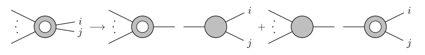
Figure 1: Diagram illustrating factorisation of one-loop matrix element. In a singly unresolved limit, the $(n+1)$-body one-loop matrix element tends to the sum of a $n$-body one-loop matrix element multiplied by a tree-level splitting kernel and a $n$-body tree-level matrix element multiplied by a one-loop splitting kernel. The tree-level elements are drawn as a fully filled in circle, while the one-loop elements are drawn as a donut shape.

2.3 Ansatz for the k-factor

Given that both the tree-level and one-loop level matrix element factorise in the soft and collinear limits, we can rewrite the $(n+1)$-body k-factor in these limits as

$$k_{n+1} \longrightarrow\dfrac{X_{ijk}^{0}|\mathcal{M}^{(n,1)}|^{2}+X_{ijk}^{1,F}|\mathcal{M}^{(n,0)}|^{2}}{X_{ijk}^{0}|\mathcal{M}^{(n,0)}|^{2}}$$

$$k_{n+1} \longrightarrow\dfrac{|\mathcal{M}^{(n,1)}|^{2}}{|\mathcal{M}^{(n,0)}|^{2}}+\dfrac{X_{ijk}^{1,F}}{X_{ijk}^{0}}$$ (5)

$$k_{n+1} \longrightarrow k_{n}+\dfrac{X_{ijk}^{1,F}}{X_{ijk}^{0}}\,.$$

where we see that the k-factor tends to a sum of the reduced k-factor, $k_{n}$, and a ratio of antenna functions. By summing over ratios of antenna functions for all limits of a given process, we can construct an ansatz for the k-factor over all of phase-space. This informs our ansatz for the k-factor, which can be given as

$$k_{n+1}=C_{0}+\sum_{\{ijk\}}C_{ijk}\dfrac{X_{ijk}^{1,F}}{X_{ijk}^{0}}\,$$ (6)

where $C_{0}$ and $C_{ijk}$ are coefficients fitted by the neural network. $C_{0}$ is an additive term aiming to model the reduced k-factor, and $C_{ijk}$ are multiplying the ratio of antenna functions to fit the single collinear, and soft limits in multiple regions of phase-space. The sum over $\{ijk\}$ denotes the sum over the relevant permutations of final-state partons. This sum allows the neural network to make use of all the provided antenna functions to make an approximation of the colour-summed matrix element. Outside of the soft and collinear limits, the ansatz makes use of the excellent interpolation abilities of neural networks to fit the k-factor in the well-behaved regions of phase-space. This is possible because the antenna functions are not singular outside of these limits. The full set of antenna functions which we implement into our model is given in Appendix B.

Since the k-factor has infrared divergences arising from unresolved partons in the final-state being removed, and with the appropriate antenna functions accounting for the logarithmic divergences from the loop momenta, the challenging task of fitting a rapidly varying function over phase-space is reduced to fitting a group of well-behaved coefficients that dictate how to suitably utilise the antenna functions.

2.4 Building the neural network emulator

Dataset generation

Phase-space is sampled uniformly using the RAMBO algorithm Kleiss:1985gy with a centre-of-mass energy $\sqrt{s_{\mathrm{com}}}=1000$ GeV. The global phase-space generation cut is set to $y_{\mathrm{cut}}=0.0001$. We have shown in Ref. Maitre:2021uaa that the accuracy of the emulation is not greatly affected by the generation cut but that the extrapolation performance is increased with a more inclusive cut, so we have chosen this value. F AST J ET Cacciari:2011ma ; noel_dawe_2021_4446849 is used to exclusively ($d_{\mathrm{cut}}=0.01\times s_{\mathrm{com}}$) cluster final-state jets with the $e^{+}e^{-}$ $k_{t}$ algorithm such that there is at most a single unresolved parton.

For each phase-space point generated, we sample a renormalisation scale, $\log(\mu_{R})$, from a uniform distribution with end points at $[\log(\sqrt{s_{\mathrm{com}}}/4),\log(4\sqrt{s_{\mathrm{com}}})]$. In other words, we sample the renormalisation scale logarithmically. We observe that the neural network manages to learn the renormalisation scale dependence well, therefore opt to sample $\mu_{R}$ in a wider range than is usually used for the conventional scale variations which varies $\mu_{R}$ up and down by factors of 2.

Generated phase-space points are fed to M AD G RAPH Alwall:2014hca ; Hirschi:2011pa to compute the tree-level and one-loop level matrix elements (using M AD L OOP ). For each phase-space point, we use the corresponding renormalisation scale sampled and evaluate the strong coupling constant at this scale using the NNPDF-4.0 NNLO PDF set NNPDF:2021njg with the LHAPDF6 interface Buckley:2014ana . All external particles are treated as massless and $m_{Z}=91.188$ GeV.

We generate 1100k data points in total, using 100k points for training and validation (80:20 split), leaving 1 million points for independent evaluation of model performance. Training on a limited dataset is a realistic scenario for processes which are prohibitively expensive, and we show that it is possible to build an accurate emulator with the relatively small number of data points. Note that because we are sampling $\mu_{R}$ along with phase-space simultaneously, there is an extra dimension in the sampled space. This means that the 100k training points we have are not comparable to 100k training points if we had not sampled over $\mu_{R}$. In practice, we have found that sampling over $\mu_{R}$ has a small impact on accuracy but opt to go this route to have the flexibility to predict over a range of $\mu_{R}$.

Inputs to model

As inputs to the neural network we provide the 4-momenta of all final-state partons. The renormalisation scale enters the network as $\log(\mu_{R})$ as we expect the dependence on $\mu_{R}$ to be in the form of a logarithm. Following Ref. Maitre:2021uaa we include the phase-space mapping variables to aid the network in learning the reduced matrix element information. More specifically, we include as inputs $r$ and $\rho$ from Ref. Kosower:1997zr

$$r_{ijk} =\dfrac{s_{jk}}{s_{ij}+s_{jk}}$$ (7)

$$\rho_{ijk} =\sqrt{1+\dfrac{4r(1-r)s_{ij}s_{jk}}{s_{ijk}s_{ik}}}\,,$$ (8)

where $i$ and $k$ are the hard radiating partons, and $j$ is the unresolved parton. We include the subscript _ijk on $r$ and $\rho$ to represent the explicit dependence on the specific set of momenta used to calculate them. To improve training, we transform these variables as $r\rightarrow\log(r)$ and $\rho\rightarrow\log(\rho-(1-\varepsilon))$, where $\varepsilon$ is a small constant added to improve the numerical stability. It is taken to be $\varepsilon=10^{-8}$. An additional input that we have observed to increase accuracy of the emulator are the Mandelstam kinematic invariants. These are fed into the model as $\log(s_{ij})$ for all pairs of final-state particles. All inputs are standardised to zero mean and unit variance.

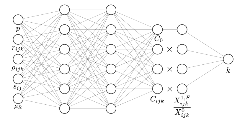
Figure 2: A schematic diagram of the neural network emulator. The emulator is a dense neural network with inputs: phase-space points, $p$, momenta mapping variables, $r_{ijk}$ and $\rho_{ijk}$, and kinematic invariants, $s_{ij}$. The outputs of the network are the fitted coefficients, $C_{0}$ and $C_{ijk}$, as given in (6).

Outputs of model

The outputs of the neural network are the fitted coefficients $C_{0}$ and $C_{ijk}$ in (6), which when combined with the antenna functions produces an approximation of the k-factor. We then recover the one-loop matrix element by multiplying by the corresponding tree-level matrix element. We do not provide the tree-level matrix element in the emulator as the evaluation time is generally much lower than that of the one-loop matrix element, and it is usual for one-loop matrix elements to be evaluated at phase-space point sets where the tree-level matrix element has already been unweighted, so that only the k-factor is required.

To train the network we we compare the target k-factors from M AD G RAPH to the predictions from the neural network in the loss function by providing the network with the antenna functions. The target distribution is standardised to zero mean and unit variance. Since the k-factors are of order unity we do not need to do any additional pre-processing to aid the network in training.

Neural network architecture

A schematic of the neural network model is given in Fig. 2. We build the neural network emulator with Keras chollet2015keras and TensorFlow tensorflow2015-whitepaper . The emulator is a dense neural network with three hidden layers of 64 nodes each. This network size was chosen with consideration given to the number of training samples and to reduce the discrepancy between training and validation loss (i.e. a larger network is more prone to overfitting on the training set if there is insufficient data to fit the additional weights). For the remaining hyperparameters we summarise the network architecture in Table 1.

Table 1: Hyperparameters of the neural network and their values.

Parameter	Value
Hidden layers	3
Nodes in hidden layers	[64, 64, 64]
Activation function	$\operatorname{swish}$ 2017arXiv170203118E ; 2017arXiv171005941R
Weight initialiser	Glorot uniform Glorot10understandingthe
Loss function	MAE (k-factor), MSE (one-loop matrix element)
Batch size	256
Optimiser	Adam kingma2017adam
Learning rate	$10^{-3}$
Callbacks	EarlyStopping, RatioEarlyStopping, ReduceLROnPlateau

We choose to use the mean absolute error (MAE) as the loss function for training because it is precisely the error measure we would like to minimise. The error for one prediction is given as

$$k_{\mathrm{true}}-k_{\mathrm{pred}}=\dfrac{|\mathcal{M}^{(n,1)}|^{2}_{\mathrm{true}}-|\mathcal{M}^{(n,1)}|^{2}_{\mathrm{pred}}}{|\mathcal{M}^{(n,0)}|^{2}_{\mathrm{true}}}=\Delta\,,$$ (9)

where the error in the one-loop matrix element normalised by the tree-level matrix element is what we want the neural network to minimise. Since k-factors are a ratio of matrix elements, the numerical values it can take are not unique for a given value of the tree-level matrix element and/or one-loop matrix element. For example, for two similar values of the k-factor, the scales of the matrix elements going into each ratio may be vastly different. To ensure that the network remains accurate for large values of the tree-level matrix element, where corresponding corrections contribute more to the total cross-section, we weight the training points by

$$w_{i}=\log\left(\dfrac{|\mathcal{M}^{(n,0)}|^{2}_{i}}{\min(|\mathcal{M}^{(n,0)}|^{2}_{i})}\right)\,,$$ (10)

where the $i$ index denotes individual training samples. Although we use the MAE on the k-factors as the training loss, we terminate model training based on the one-loop matrix element accuracy. This is done by monitoring the mean squared error (MSE) between the model prediction and corresponding truth value at the end of each training epoch. This takes advantage of the compact k-factor distributions for training purposes, but bases model selection on the performance for the physical one-loop matrix elements.

To reduce the effects of overfitting we have two EarlyStopping criteria: the first is to stop training once the validation loss has not improved in 100 epochs, and the second is a RatioEarlyStopping which terminates training if the ratio of training loss to validation loss drops below a certain threshold. We take this threshold to be $0.9$. We also use the ReduceLROnPlateau callback as a way to adapt the learning rate during training. The learning rate is reduced by a factor of 0.7 whenever validation loss plateaus with a patience of 20 epochs. We find that with these hyperparameters we achieve a balance of reducing overfitting and quick training times. On average the models train in approximately 20 minutes on an Nvidia P100 GPU.

Although we build and train our model using TensorFlow, we deploy the model using the Open Neural Network Exchange (ONNX) runtime onnxruntime with the CUDA execution provider to run predictions on an Nvidia P100 GPU. With the optimised operations in the ONNX runtime, we see that compared to TensorFlow the model inference time is reduced by an order of magnitude or more. Another advantage is that it provides flexibility to move the pipeline away from TensorFlow on $\mathtt{Python}$ to a more generic interface to the neural network model. One example would be to integrate the ONNX model into a C++ workflow for use with current event generators to replace the one-loop provider with a neural network emulator. This workflow was recently seen for tree-level matrix element emulation within the S herpa framework in the context of accelerating the generation of unweighted events Janssen:2023ahv .

In addition to the CUDA execution provider, we will use the ONNX runtime CPU execution provider to compare with M AD G RAPH for a comparison of single CPU core performance. This will be the closest to a real world benchmark as event generators typically generate events on a single core.

Although we find that the neural network models converge well, to account for stochasticity in the training, the random initialisation of model parameters, and to reduce variance on predictions, we initialise 20 models for training and use the mean of these models as our model prediction. This ensembling will also give a measure of the uncertainty due to the neural network optimisation, by using the standard deviation of the 20 replica model predictions.

We plot in Figure 3 the losses of the 20 replica models for the 5 jet process, where we have plotted the loss for the k-factor (MAE) and the one-loop matrix element (MSE). We can see that the models have all converged to a similar point when training is terminated. The noise in the validation loss at the beginning of training can be attributed to the fitting of the coefficients: when the model is learning how to pick the relevant combination of antenna functions there can be large variations in the prediction, however, the variations become much smaller once the model learns the factorisation properties and converges. We can see the variations in the validation loss are small at the end of training, and that there is not a large discrepancy between the training and validation losses, as enforced by the RatioEarlyStopping callback. Furthermore, since the training of the network is dictated by the MAE loss, the more apparent noise in the MSE loss was foreseeable as the losses are unlikely to respond the same way to updates of the model weights.

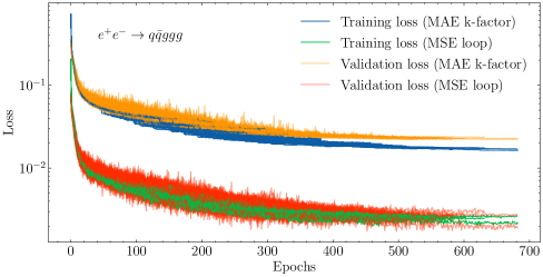
Figure 3: Training and validation losses of the 20 independent initialisations of the ensemble replicas plotted as individual curves for the 5 parton model. We plot the MAE loss for the k-factor and the MSE loss for the one-loop matrix element. The scale difference between the MAE and MSE losses is a consequence of the form of the loss functions and is not surprising. We see that the replica models all converge to similar point with the validation loss being close to the training loss when training is terminated. The step feature in the training loss is due to the ReduceLROnPlateau callback.

3 Results

In this section we present results for our NLO QCD k-factor emulator for $e^{+}e^{-}$ annihilation into up to 5-jets. First we show a comparison between our model described in Section 2.4 which we label ‘antenna’, and a ‘naive’ model with no factorisation properties built into the emulator: a densely connected neural network with the parameters given in Table 1 that directly predicts the k-factor. For the ‘naive’ models we train with the MAE on the k-factors as the loss function with no modifications and terminate training based on this loss. As with the ‘antenna’ models, we also ensemble 20 individual replica models for the ‘naive’ model predictions. In Figure 4 we compare histograms of $\Delta$ for all final-state multiplicities between these two models. It is immediately clear that building in the factorisation structure of the matrix elements greatly increases accuracy, with increasing relative improvements for the higher multiplicity cases. The ‘antenna’ error distributions are symmetric, strongly peaked around the ideal value of 0, and with tails falling off rapidly. We see the general trend of increasing multiplicity decreases accuracy, however we observe that the bulk of the 5 jet final-state is within percent accuracy and with the lower multiplicities well below this.

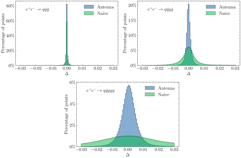
Figure 4: Error distribution in terms of $\Delta$ for all multiplicities. ‘Antenna’ model is as described in this article, and ‘naive’ model is a simple densely connected neural network model without any factorisation properties built in. We keep the horizontal axis scale fixed for all subplots to make it easier to compare accuracy across the different multiplicities.

To show that we are accurate across the entire span of the tree-level matrix elements, and to have a closer inspection of the tails of the $\Delta$ distribution, we plot a 2d histogram of $\Delta$ against the value of $|\mathcal{M}^{(5,0)}|^{2}$ in Figure 5. The bulk of phase-space points are contained in the high population bins depicted in yellow, representing the peaked distribution seen in Figure 4, whereas the green to purple coloured bins represent the tails of the low population $\Delta$ distribution. We see that the accuracy stays contained inside a band and does not flare out as the magnitude of the tree-level matrix element increases. This shows that we manage to fit the k-factor even in the infrared and collinear limits where the tree-level matrix element becomes large. On the right-hand side subplot we plot the distribution of the tree-level matrix elements where we can see that that even with relatively few training points in the tails, the emulator is still able to predict these regions as well as where there is more abundant data.

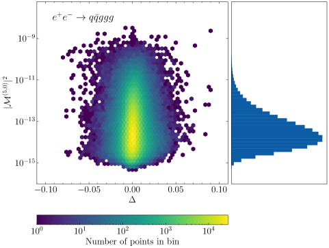
Figure 5: Left: $\Delta$ error distribution plotted against the tree-level matrix element. Yellow bins indicates high density regions of points and purple bins indicates single points. Right: marginal distribution of tree-level matrix elements. This illustrates that the network is able to reproduce a good approximation across all sampled phase-space.

In Figure 6, we show that our emulator has learned the renormalisation scale dependence, independent of the antenna functions. To produce a trajectory we first sample a phase-space point with the same cuts as described in Section 2.4, then we evaluate the k-factor at this phase-space point with $\mu_{R}$ varying from $\sqrt{s_{\mathrm{com}}}/8$ to $8\sqrt{s_{\mathrm{com}}}$. We choose to sample from a wider range than used for training to examine the $\mu_{R}$ extrapolation performance. After subtracting the sum of the antenna functions we see that the remainder still has a dependence on the renormalisation scale that is accurately captured by the neural network. As with the $\Delta$ distribution plots in Figure 4, there is a slight decrease in accuracy as we increase the multiplicity, however, the ratios and differences are well-behaved throughout the entirety of the trajectories inside the range of training data. The only anomaly occurs when the trajectories cross zero, causing spikes in the ratios, but the difference in truth and prediction remains well-behaved around these regions. Outside of the training range we see an acceptable extrapolation, but given that the training range is wider than the range in which the renormalisation scale is normally varied for scale variations, we do not find this problematic.

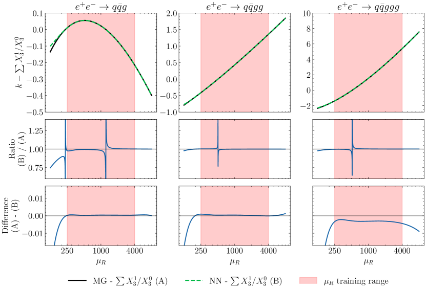
Figure 6: Renormalisation scale trajectories for all multiplicities. These trajectories are predictions of the k-factor with the sum of antenna functions subtracted to show renormalisation scale dependence in the remainder. Each trajectory is at one phase-space point sampled from RAMBO, with $\mu_{R}$ spanning the range $[\sqrt{s_{\mathrm{com}}}/8,8\sqrt{s_{\mathrm{com}}}]$. Each trajectory is composed of 1000 points. The region that $\mu_{R}$ was uniformly sampled from for training is indicated as a red band. The error bands on the NN predictions are too small to be seen.

In Figure 7 we show that we reproduce the total cross-sections over an integration of 1M phase-space points, for all multiplicities, at three different values of the renormalisation scale representing the nominal value ($\mu_{R}=\sqrt{s_{\mathrm{com}}}=1000$ GeV) and the two variations usually used to estimate scale uncertainties. Note that these phase-space points were generated independently of those in Figure 4, and that we are integrating the tree-level and one-loop interference, not the k-factor. We multiply our NLO k-factor prediction with the M AD G RAPH tree-level matrix element to reproduce the loop-matrix element for integration. The neural network errors are well below the statistical Monte Carlo integration error. By neural network error we are referring to the absolute percentage difference to the cross-section, and not the errors due to neural network optimisation. For that, we examine the variations in the 20 replica model predictions in Figure 8 where we plot the total cross-section predictions as a scatter plot. The blue band illustrated is one standard deviation of the 20 predictions made. We see that the true value of the total cross-section is within the one standard deviation band. Not shown in the figure is the Monte Carlo statistical error which as seen in Figure 7 dominates the absolute error between the NN predictions and the true value.

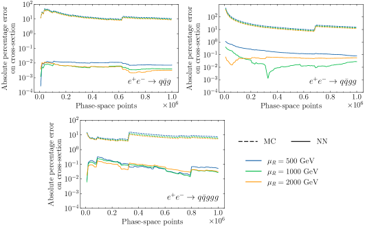
Figure 7: Error on the total cross-section across an integration of 1M phase-space points. For each multiplicity, we evaluate the matrix elements at the three values of the renormalisation scale as reported. The solid lines are the absolute percentage error in the true total cross-section and the NN predicted value. The dashed line represents the statistical Monte Carlo integration error which falls as $1/\sqrt{N}$. The jumps in error are due to large values of the matrix element being integrated.

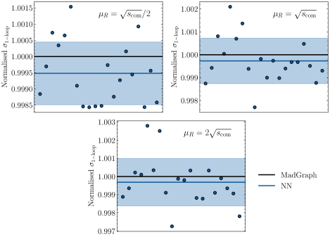
Figure 8: Scatter plot showing the variation in predictions of the 5 jet total cross-section for the 20 replicas. Total cross-sections are evaluated at the renormalisation scale quoted, and normalised by the M

AD

G

RAPH

prediction (horizontal black line). The mean prediction of the replicas is drawn as the horizontal blue line with one standard deviation illustrated by the blue band.

Since the discrepancy between the true total cross-section and NN predicted total cross-section is so small, this strongly indicates that once we fit on the relatively small training set, we can predict with good confidence on many more phase-space points to get a prediction of the cross-section before reaching the same level of error as the Monte Carlo statistical error. This can also be seen from the shape of the NN error, it is relatively constant once enough points have been integrated. This feature enables us to use our trained model to augment the dataset size by orders of magnitude beyond the size of the training set used to fit it and reduced the statistical error without compromising accuracy.

In Figure 9, we plot the evaluation time of the emulator for both the CPU and CUDA (GPU) execution providers in the ONNX runtime, as well as the reference time from M AD G RAPH . For the NN (GPU) predictions we predict on 1M phase-space points concurrently, whereas for the NN (CPU) predictions, we predict on one point at a time. The times reported are then the mean of the total evaluation times. We see that compared to M AD G RAPH , our NN emulator is faster for all multiplicities, although the advantage is greatest for the 5 jet case, with speed gains of over four orders of magnitude when utilising GPU acceleration. The advantage of using the GPU is not only from being able to batch process the predictions, it is also to leverage the auto-vectorisation tools provided by, for example TensorFlow, to accelerate the model input computations.

While the evaluation time of the GPU accelerated NNs are by far the quickest, and would be the ideal scenario for a NN emulator to be used, event generation typically occurs on CPUs where phase-space points are evaluated one at a time. This is precisely why our NN (CPU) predictions were made on single phase-points and not over batches, to showcase what the performance would be like when embedded in a typical workflow. We observe that even with this constraint, the NN emulator is much quicker in the higher multiplicity cases.

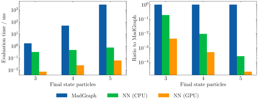
Figure 9: Left: evaluation time in milliseconds of a single phase-space point. Times quoted for M

AD

G

RAPH

are averaged over 1000 random phase-space points. Times quoted for NN are averaged over 1M random phase-space points. Right: ratio of evaluation times to M

AD

G

RAPH

. GPU used is Nvidia P100 16GB, and CPU is Intel(R) Xeon(R) Gold 6126 CPU @ 2.60GHz.

One of the main bottlenecks in the NN (CPU) prediction is using the NN ensemble to infer on single phase-space points, this is illustrated by the weak scaling in multiplicity in the left subplot of Figure 9 and is illustrated explicitly in Figure 10. Since the model architecture is identical for all multiplicities other than the final output layer, there will not be much difference in cost. Another bottleneck is the computation of model inputs, which contain large, complex expressions with many evaluations of logarithms and dilogarithms. In our $\mathtt{Python}$ implementation, the computation time of these inputs is comparable to the model inference time in the 5 jet case, as shown in Figure 10. Time taken to compute the model input scales with the final-state partons because of the increase in number of antenna functions in the ansatz to account for the large number of singular configurations, as well as a larger number of the other input variables.

For the NN (GPU) predictions, the model inference time is negligible compared to the model input computations since we take advantage of predicting on the entire batch of 1M phase-space points at once, and so once averaged across this dataset each single point takes an insignificant amount of time. The model input computations are vectorised on the GPU and so we see an order of magnitude reduction in time taken to calculate them compared to computing them on a single core of a CPU.

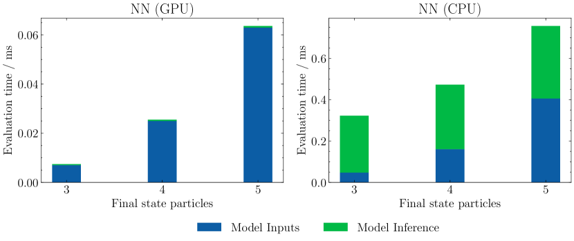
Figure 10: Breakdown of the total time taken to predict on a phase-space point (averaged over 1M predictions) into model input computations and the actual model inference for both GPU and CPU model deployments. The model inference portions in the NN (GPU) subplot are very small.

We note that our emulator retains good performance even when we go to higher multiplicity. In Ref. Badger:2022hwf the authors expressed concern about the fact that the accuracy of the surrogate model is decreasing with the multiplicity of the process. We show that by incorporating suitable physically motivated functions in the ansatz that the network accuracy drops off much less rapidly when going to higher multiplicities.

4 Conclusion

In this article we presented the extension to one-loop matrix elements of Ref. Maitre:2021uaa , where we introduced the factorisation-aware model for tree-level processes. By adapting the ingredients provided to the neural network model to a suitable set, we have been able to adapt the emulation of tree-level matrix element to the modelling of NLO k-factors. We have shown that the philosophy of incorporating relevant physics information into a regression model greatly improves accuracy of predictions even for matrix elements with a complex divergence structure.

The results presented demonstrate that predictions are at the percent level for the most demanding process, with accuracy in the infrared regions of phase-space being well-behaved. We have also shown that for relatively few training points, the model is able to learn the target function well enough such that the accumulated error due to the modelling is well below the statistical integration uncertainty of the training sample. Furthermore, the modelling uncertainty of cross-section predictions associated with optimisation of model parameters was shown to contain the truth value and therefore provides a useable estimate of the accuracy of the emulation.

In addition to being accurate, we have given evidence that the model, although optimally deployed on a GPU, is orders of magnitude quicker than traditional loop providers on a single CPU. By deploying the model with the ONNX runtime a generic interface to the neural network model is available in many programming languages, allowing it to be embedded into modern event generators which are mainly written in C++.

These facts put together provide conclusive evidence that the factorisation aware neural network model can be used to augment existing samples with additional phase-space points with confidence. Given the high compuational costs of high-multiplicity one-loop matrix elements using this data augmentation capability can further the reach of existing and future simulations for a fixed computational resource envelope.

Appendix A Finite part of singularity operators

The finite part of the Catani singularity operators can be written as

$$\mathcal{F}(\mathbf{I}^{(1)}_{ij}(\epsilon,s_{ij}))=\epsilon_{0}+\epsilon_{1}\Re{(z)}+\dfrac{1}{2}\epsilon_{2}\Re{(z^{2})}\,,$$ (11)

where

$$z=\operatorname{zlog}(\mu_{R}^{2})-\operatorname{zlog}(-s_{ij})$$ (12)

and coefficients are given as

$$\epsilon_{0} =\dfrac{\pi^{2}}{24}\,,$$

$$\epsilon_{1} =\begin{cases}-\frac{5}{6},&\text{if }ij=qg\;\text{or}\;gq\\ -\frac{3}{4},&\text{if }ij=qq\\ -\frac{11}{12},&\text{if }ij=gg\end{cases}$$ (13)

$$\epsilon_{2} =-\dfrac{1}{2}\,.$$

The $\operatorname{zlog}$ function is extending the logarithm for all real-values

$$\operatorname{zlog}(x)=\begin{cases}\log(x),&\text{if }x\geq 0\\ \log(|x|)-i\pi,&\text{otherwise}\,.\end{cases}$$ (14)

Appendix B Antenna functions

Here we tabulate the full set of antenna functions which we build into our emulation model. In the main article we refer to the antenna functions as $X_{ijk}^{\ell}$ which in practice is replaced with specific antennae containing either $qg\bar{q}$, $qgg$ ($\bar{q}gg$), or $ggg$, which are referred to as $A$, $D$, and $F$, respectively. The antennae listed in Table 2 are sufficient to describe all infrared singularities in the partonic processes we consider.

$n$	Tree-level antenna	One-loop antenna	{$i$, $j$, $k$} permutations
3 $(q\bar{q}g)$	$A_{3}^{0}(q,g,\bar{q})$	$A_{3}^{1}(q,g,\bar{q})$	(1, 3, 2)
4 $(q\bar{q}gg)$	$A_{3}^{0}(q,g,\bar{q})$ $D_{3}^{0}(q,g,g)$	$A_{3}^{1}(q,g,\bar{q})$ $D_{3}^{1}(q,g,g)$	(1, 3, 2), (1, 4, 2) (1, 3, 4), (2, 3, 4)
5 $(q\bar{q}ggg)$	$A_{3}^{0}(q,g,\bar{q})$ $D_{3}^{0}(q,g,g)$ $F_{3}^{0}(g,g,g)$	$A_{3}^{1}(q,g,\bar{q})$ $D_{3}^{1}(q,g,g)$ $F_{3}^{1}(g,g,g)$	(1, 3, 2), (1, 4, 2), (1, 5, 2) (1, 3, 4), (1, 3, 5), (1, 4, 5), (2, 3, 4), (2, 3, 5), (2, 4, 5), (3, 4, 5)

Table 2: List of antenna functions we use for each process, and the full list of {$i$, $j$, $k$} permutations, where $q=1$, $\bar{q}=2$, $g=3,4,5$.

References

- (1) D. Maître and H. Truong, A factorisation-aware Matrix element emulator, JHEP 11 (2021) 066 [2107.06625].
- (2) P. Azzi et al., Report from Working Group 1: Standard Model Physics at the HL-LHC and HE-LHC, CERN Yellow Rep. Monogr. 7 (2019) 1 [1902.04070].
- (3) K. Bloom, V. Boisvert, D. Britzger, M. Buuck, A. Eichhorn, M. Headley et al., Climate impacts of particle physics, in 2022 Snowmass Summer Study, 3, 2022 [2203.12389].
- (4) S. Badger and J. Bullock, Using neural networks for efficient evaluation of high multiplicity scattering amplitudes, JHEP 06 (2020) 114 [2002.07516].
- (5) J. Aylett-Bullock, S. Badger and R. Moodie, Optimising simulations for diphoton production at hadron colliders using amplitude neural networks, 2106.09474.
- (6) S. Badger, A. Butter, M. Luchmann, S. Pitz and T. Plehn, Loop Amplitudes from Precision Networks, 2206.14831.
- (7) F. Bishara, A. Paul and J. Dy, High-precision regressors for particle physics, 2302.00753.
- (8) E. Bothmann, A. Buckley, I.A. Christidi, C. Gütschow, S. Höche, M. Knobbe et al., Accelerating LHC event generation with simplified pilot runs and fast PDFs, 2209.00843.
- (9) J. Bendavid, Efficient Monte Carlo Integration Using Boosted Decision Trees and Generative Deep Neural Networks, 1707.00028.
- (10) M.D. Klimek and M. Perelstein, Neural Network-Based Approach to Phase Space Integration, SciPost Phys. 9 (2020) 053 [1810.11509].
- (11) E. Bothmann, T. Janßen, M. Knobbe, T. Schmale and S. Schumann, Exploring phase space with Neural Importance Sampling, SciPost Phys. 8 (2020) 069 [2001.05478].
- (12) B. Stienen and R. Verheyen, Phase Space Sampling and Inference from Weighted Events with Autoregressive Flows, SciPost Phys. 10 (2021) 038 [2011.13445].
- (13) I.-K. Chen, M. Klimek and M. Perelstein, Improved neural network monte carlo simulation, SciPost Physics 10 (2021) .
- (14) T. Heimel, R. Winterhalder, A. Butter, J. Isaacson, C. Krause, F. Maltoni et al., MadNIS – Neural Multi-Channel Importance Sampling, 2212.06172.
- (15) S. Carrazza and F.A. Dreyer, Lund jet images from generative and cycle-consistent adversarial networks, Eur. Phys. J. C 79 (2019) 979 [1909.01359].
- (16) E. Bothmann and L. Debbio, Reweighting a parton shower using a neural network: the final-state case, JHEP 01 (2019) 033 [1808.07802].
- (17) K. Dohi, Variational Autoencoders for Jet Simulation, 2009.04842.
- (18) C. Gao, S. Höche, J. Isaacson, C. Krause and H. Schulz, Event Generation with Normalizing Flows, Phys. Rev. D 101 (2020) 076002 [2001.10028].
- (19) S. Otten, S. Caron, W. de Swart, M. van Beekveld, L. Hendriks, C. van Leeuwen et al., Event Generation and Statistical Sampling for Physics with Deep Generative Models and a Density Information Buffer, 1901.00875.
- (20) B. Hashemi, N. Amin, K. Datta, D. Olivito and M. Pierini, LHC analysis-specific datasets with Generative Adversarial Networks, 1901.05282.
- (21) R. Di Sipio, M. Faucci Giannelli, S. Ketabchi Haghighat and S. Palazzo, DijetGAN: A Generative-Adversarial Network Approach for the Simulation of QCD Dijet Events at the LHC, JHEP 08 (2019) 110 [1903.02433].
- (22) A. Butter, T. Plehn and R. Winterhalder, How to GAN LHC Events, SciPost Phys. 7 (2019) 075 [1907.03764].
- (23) F. Bishara and M. Montull, (Machine) Learning amplitudes for faster event generation, 1912.11055.
- (24) M. Backes, A. Butter, T. Plehn and R. Winterhalder, How to GAN Event Unweighting, 2012.07873.
- (25) A. Butter, S. Diefenbacher, G. Kasieczka, B. Nachman and T. Plehn, GANplifying Event Samples, 2008.06545.
- (26) Y. Alanazi et al., Simulation of electron-proton scattering events by a Feature-Augmented and Transformed Generative Adversarial Network (FAT-GAN), 2001.11103.
- (27) B. Nachman and J. Thaler, Neural resampler for Monte Carlo reweighting with preserved uncertainties, Phys. Rev. D 102 (2020) 076004 [2007.11586].
- (28) K. Danziger, T. Janßen, S. Schumann and F. Siegert, Accelerating Monte Carlo event generation – rejection sampling using neural network event-weight estimates, SciPost Phys. 12 (2022) 164 [2109.11964].
- (29) T. Janßen, D. Maître, S. Schumann, F. Siegert and H. Truong, Unweighting multijet event generation using factorisation-aware neural networks, 2301.13562.
- (30) H. Truong, “Fame-antenna.” https://github.com/htruong0/fame_antenna, 2023.
- (31) P. Baldi, K. Cranmer, T. Faucett, P. Sadowski and D. Whiteson, Parameterized neural networks for high-energy physics, Eur. Phys. J. C 76 (2016) 235 [1601.07913].
- (32) A. Ghosh, B. Nachman and D. Whiteson, Uncertainty-aware machine learning for high energy physics, Phys. Rev. D 104 (2021) 056026 [2105.08742].
- (33) S. Catani and M. Seymour, A General algorithm for calculating jet cross-sections in NLO QCD, Nucl. Phys. B 485 (1997) 291 [hep-ph/9605323].
- (34) A. Gehrmann-De Ridder, T. Gehrmann and E.W.N. Glover, Antenna subtraction at NNLO, JHEP 09 (2005) 056 [hep-ph/0505111].
- (35) Z. Bern, V. Del Duca, W.B. Kilgore and C.R. Schmidt, The infrared behavior of one loop QCD amplitudes at next-to-next-to leading order, Phys. Rev. D 60 (1999) 116001 [hep-ph/9903516].
- (36) Z. Bern, L.J. Dixon, D.C. Dunbar and D.A. Kosower, One loop n point gauge theory amplitudes, unitarity and collinear limits, Nucl. Phys. B 425 (1994) 217 [hep-ph/9403226].
- (37) Z. Bern and G. Chalmers, Factorization in one loop gauge theory, Nucl. Phys. B 447 (1995) 465 [hep-ph/9503236].
- (38) D.A. Kosower, All order collinear behavior in gauge theories, Nucl. Phys. B 552 (1999) 319 [hep-ph/9901201].
- (39) D.A. Kosower, Antenna factorization of gauge theory amplitudes, Phys. Rev. D 57 (1998) 5410 [hep-ph/9710213].
- (40) D.A. Kosower, Multiple singular emission in gauge theories, Phys. Rev. D 67 (2003) 116003 [hep-ph/0212097].
- (41) R. Kleiss, W. Stirling and S. Ellis, A New Monte Carlo Treatment of Multiparticle Phase Space at High-energies, Comput. Phys. Commun. 40 (1986) 359.
- (42) M. Cacciari, G.P. Salam and G. Soyez, FastJet User Manual, Eur. Phys. J. C 72 (2012) 1896 [1111.6097].
- (43) N. Dawe, E. Rodrigues, H. Schreiner, B. Ostdiek, D. Kalinkin, M. R. et al., scikit-hep/pyjet: Version 1.8.2, Jan., 2021. 10.5281/zenodo.4446849.
- (44) J. Alwall, R. Frederix, S. Frixione, V. Hirschi, F. Maltoni, O. Mattelaer et al., The automated computation of tree-level and next-to-leading order differential cross sections, and their matching to parton shower simulations, JHEP 07 (2014) 079 [1405.0301].
- (45) V. Hirschi, R. Frederix, S. Frixione, M.V. Garzelli, F. Maltoni and R. Pittau, Automation of one-loop QCD corrections, JHEP 05 (2011) 044 [1103.0621].
- (46) NNPDF collaboration, The path to proton structure at 1% accuracy, Eur. Phys. J. C 82 (2022) 428 [2109.02653].
- (47) A. Buckley, J. Ferrando, S. Lloyd, K. Nordström, B. Page, M. Rüfenacht et al., LHAPDF6: parton density access in the LHC precision era, Eur. Phys. J. C 75 (2015) 132 [1412.7420].
- (48) F. Chollet et al., “Keras.” https://keras.io, 2015.
- (49) M. Abadi, A. Agarwal, P. Barham, E. Brevdo, Z. Chen, C. Citro et al., TensorFlow: Large-scale machine learning on heterogeneous systems, 2015.
- (50) S. Elfwing, E. Uchibe and K. Doya, Sigmoid-Weighted Linear Units for Neural Network Function Approximation in Reinforcement Learning, arXiv e-prints (2017) arXiv:1702.03118 [1702.03118].
- (51) P. Ramachandran, B. Zoph and Q.V. Le, Searching for Activation Functions, arXiv e-prints (2017) arXiv:1710.05941 [1710.05941].
- (52) X. Glorot and Y. Bengio, Understanding the difficulty of training deep feedforward neural networks, in In Proceedings of the International Conference on Artificial Intelligence and Statistics (AISTATS’10). Society for Artificial Intelligence and Statistics, 2010.
- (53) D.P. Kingma and J. Ba, Adam: A method for stochastic optimization, 2017.
- (54) O.R. developers, “Onnx runtime.” https://onnxruntime.ai/, 2022.