On the non-linear stability of the Cosmological region of the Schwarzschild-de Sitter spacetime

Abstract

The non-linear stability of the sub-extremal Schwarzschild-de Sitter spacetime in the stationary region near the conformal boundary is analysed using a technique based on the extended conformal Einstein field equations and a conformal Gaussian gauge. This strategy relies on the observation that the Cosmological stationary region of this exact solution can be covered by a non-intersecting congruence of conformal geodesics. Thus, the future domain of dependence of suitable spacelike hypersurfaces in the Cosmological region of the spacetime can be expressed in terms of a conformal Gaussian gauge. A perturbative argument then allows us to prove existence and stability results close to the conformal boundary and away from the asymptotic points where the Cosmological horizon intersects the conformal boundary. In particular, we show that small enough perturbations of initial data for the sub-extremal Schwarzschild-de Sitter spacetime give rise to a solution to the Einstein field equations which is regular at the conformal boundary. The analysis in this article can be regarded as a first step towards a stability argument for perturbation data on the Cosmological horizons.

1 Introduction

One of the key problems in mathematical General Relativity is that of the non-linear stability of black hole spacetimes. This problem is challenging for its mathematical and physical features. Most efforts to establish the non-linear stability of black hole spacetimes in both the asymptotically flat and Cosmological setting have, so far, relied on the use of vector field methods —see e.g. [4].

The results in [6, 7, 27] show that the conformal Einstein field equations are a powerful tool for the analysis of the stability of vacuum asymptotically simple spacetimes. They provide a system of field equations for geometric objects defined on a four-dimensional Lorentzian manifold $(\mathcal{M},{\bm{g}})$, the so-called unphysical spacetime, which is conformally related to a spacetime $(\tilde{\mathcal{M}},\tilde{{\bm{g}}})$, the so-called physical spacetime, satisfying the Einstein field equations. The usefulness of the conformal transformation relies on the fact that global problems for the physical spacetimes are recasted as local existence problems for the unphysical spacetime. The conformal Einstein field equations constitute a system of differential conditions on the curvature tensors with respect to the Levi-Civita connection of ${\bm{g}}$ and the conformal factor $\Xi$. The original formulation of the equations, see e.g. [5], requires the introduction of so-called gauge source functions to construct evolution equations. An alternative approach to gauge fixing is to adapt the analysis to a congruence of curves. A natural candidate for a congruence is given by conformal geodesics —a conformally invariant generalisation of the standard notion of geodesics. Using these curves to fix the gauge allows to define a conformal Gaussian system. To combine this gauge choice with the conformal Einstein field equations it is necessary to make use of a more general version of the latter —the extended conformal Einstein field equations. The extended conformal field equations have been used to obtain an alternative proof of the semiglobal non-linear stability of the Minkowski spacetime and of the global non-linear stability of the de Sitter spacetime —see [20].

In view of the success of conformal methods to analyse the global properties of asymptotically simple spacetimes, it is natural to ask whether a similar strategy can be used to study the non-linear stability of black hole spacetimes. This article gives a first step in this direction by analysing certain aspects of the conformal structure of the sub-extremal Schwarzschild-de Sitter spacetime which can be used, in turn, to adapt techniques from the asymptotically simple setting to the black hole case.

The Schwarzschild-de Sitter spacetime. The Schwarzschild-de Sitter spacetime is a spherically symmetric solution to the vacuum Einstein field equations with Cosmological constant. This spacetime depends on the de Sitter-like value of the Cosmological constant $\lambda$ and on the mass $m$ of the black hole. Assuming spherical symmetry almost completely singles out the Schwarzschild-de Sitter spacetimes among the vacuum solutions to the Einstein field equations with de Sitter-like Cosmological constant. The other admissible solution is the Nariai spacetime —see e.g. [26]. In the Schwarzschild-de Sitter spacetime, the relation between the mass and the Cosmological constant determines the location of the Cosmological and black hole horizons —see e.g. [14].

The Schwarzschild-de Sitter spacetime solution can be studied by means of the extended conformal Einstein field equations —see [13]. This is in fact a spacetime with a smooth conformal extension towards the future (or past). Since the Cosmological constant takes a de Sitter-like value, the conformal boundary of the spacetime is spacelike and moreover, there exists a conformal representation in which the induced $3$-metric on the conformal boundary $\mathscr{I}$ is homogeneous. Thus, it is possible to integrate the extended conformal field equations along single conformal geodesics —see [12].

In this article, we analyse the sub-extremal Schwarzschild-de Sitter spacetime as a solution to the extended conformal Einstein field equations and use the insights to prove existence and stability results.

The main result. The metric of the Schwarzschild-de Sitter spacetime can be expressed in standard coordinates by the line element

$$\mathring{\tilde{{\bm{g}}}}=-\bigg{(}1-\frac{2m}{r}-\frac{\lambda}{3}r^{2}\bigg{)}\mathbf{d}t\otimes\mathbf{d}t+\bigg{(}1-\frac{2m}{r}-\frac{\lambda}{3}r^{2}\bigg{)}^{-1}\mathbf{d}r\otimes\mathbf{d}r+r^{2}\bm{\sigma}.$$ (1)

In this article we restrict our attention to a choice of the parameters $\lambda$ and $m$ for which the exact solution is sub-extremal —see Section 3 for a definition of this notion. The sub-extremal Schwarzschild-de Sitter spacetime has three horizons. Of particular interest for our analysis is the Cosmological horizon which bounds a region (the Cosmological region) of the spacetime in which the roles of the coordinates $t$ and $r$ reversed. In analogy to the de Sitter spacetime, the Cosmological region has an asymptotic region admitting a smooth conformal extension with spacelike conformal boundary. In the following, our analysis will be solely concerned with the Cosmological region.

The analysis of the conformal properties of the Schwarzschild-de Sitter spacetime allows us to formulate a result concerning the existence of solutions to the initial value problem for the Einstein field equations with de Sitter-like cosmological constant which can be regarded as perturbations of portions of the initial hypersurface at $\mathcal{S}_{\star}\equiv\{r=r_{\star}\}$ in the Cosmological region of the spacetime. In this region these hypersurfaces are spacelike and the coordinate $t$ is spatial. In the following, let ${\mathcal{R}}_{\bullet}$ denote finite cylinder within $\mathcal{S}_{\star}$ for which $|t|<t_{\bullet}$ for some suitable positive constant $t_{\bullet}$. Let $D^{+}({\mathcal{R}}_{\bullet})$ denote the future domain of dependence of ${\mathcal{R}}_{\bullet}$. For the Schwarzschild-de Sitter spacetime such a region is unbounded towards the future and admits a smooth conformal extension with a spacelike conformal boundary.

Our main result can be stated as:

Theorem.

Given smooth initial data $(\tilde{{\bm{h}}},\tilde{{\bm{K}}})$ for the vacuum Einstein field equations on ${\mathcal{R}}_{\bullet}\subset\mathcal{S}_{\star}$ which is suitably close (as measured by a suitable Sobolev norm) to the data implied by the metric (1) in the Cosmological region of the spacetime, there exists a smooth metric $\tilde{{\bm{g}}}$ defined over the whole of $D^{+}({\mathcal{R}}_{\bullet})$ which is close to $\mathring{\tilde{{\bm{g}}}}$, solves the vacuum Einstein field equations with positive Cosmological constant and whose restriction to ${\mathcal{R}}_{\bullet}$ implies the initial data $(\tilde{{\bm{h}}},\tilde{{\bm{K}}})$. The metric $\tilde{{\bm{g}}}$ admits a smooth conformal extension which includes a spacelike conformal boundary.

A detailed version of this theorem will be given in Section 6.

Observe that the above result is restricted to the future domain of dependence of a suitable portion ${\mathcal{R}}_{\bullet}$ of the spacelike hypersurface $\mathcal{S}_{\star}$. The reason for this restriction is the degeneracy of the conformal structure at the asymptotic points of the Schwarzschild-de Sitter spacetime where the conformal boundary, the Cosmological horizon and the singularity seem to “meet” —see [13]. In particular, at these points the background solution experiences a divergence of the Weyl curvature. This singularity is remarkably similar to that produced by the ADM mass at spatial infinity in asymptotically flat spacetimes —see e.g. [27], chapter 20. It is thus conceivable that an approach analogous to that used in the analysis of the problem of spatial infinity in [9] may be of help to deal with this singular behaviours of the conformal structure.

The ultimate aim of the programme started in this article is to obtain a proof of the stability of the Schwarzschild-de Sitter spacetime for data prescribed on the Cosmological horizon. Key to this end is the observation that the hypersurfaces of constant coordinate $r$, $\mathcal{S}_{\star}$, can be chosen to be arbitrarily close to the horizon. As such, an adaptation of the optimal local existence results for the characteristic initial value problem developed in [21] —see also [15]— should allow to evolve from the Cosmological horizon to a hypersurface $\mathcal{S}_{\star}$. These ideas will be developed in a subsequent article.

It should be stressed that the spacetimes obtained as a result of our perturbative analysis are dynamic —in the sense that, generically, they will not have Killing vectors. This is a consequence of the fact that initial data sets for the Einstein field equations admitting solutions to the Killing initial data (KID) equations are non-generic —see e.g. [1]. Whether it is possible to use conformal Gaussian systems to describe more generic, dynamic, black hole spacetimes (in both the asymptotically flat and Cosmological setting) is an interesting and challenging open question which would benefit from the input of numerical simulations.

Other approaches. The non-linear stability of the Schwarzschild-de Sitter spacetime has been studied by means of the vector field methods that have proven successful in the analysis of asymptotically flat black holes —see e.g. [23, 24, 25]. An alternative approach has made use of methods of microlocal analysis in the steps of Melrose’s school of geometric scattering —see [16, 17]. The methods developed in the present article aim at providing a complementary approach to the non-linear stability of this Cosmological black hole spacetime. The interrelation between the results obtained in this article and those obtained by vector field methods and microlocal analysis will be discussed elsewhere.

Outline of the article

This article is organised as follows. In Section 2 we provide a succinct discussion of the tools of conformal geometry that will be used in our analysis —the extended conformal Einstein equations and conformal geodesics. Moreover, it also discusses the notion of a conformal Gaussian gauge and provides a hyperbolic reduction of the extended conformal equations in terms of this type of gauge. Section 3 summarises the general properties of the Schwarzschild-de Sitter spacetime that will be used in our constructions. Section 4 describes the construction of a suitable conformal Gaussian gauge system starting from data prescribed on hypersurfaces of constant coordinate $r$ on the Cosmological region of the Schwarzschild-de Sitter spacetime. Section 5 provides a discussion of the key properties of the Schwarzschild-de Sitter spacetime in the conformal Gaussian gauge of Section 4. The main existence and stability results of this article are presented in Section 6. We conclude the article with some conclusions and outlook in Section 7.

Notations and conventions

In what follows, the low-case Latin letters $a,\,b,\,c\ldots$ will denote spacetime abstract tensorial indices, while $i,\,j,\,k,\ldots$ are spatial tensorial indices ranging from 1 to 3. By contrast, the low-case Greek letters $\mu,\,\nu,\,\lambda,\ldots$ and $\alpha,\,\beta,\gamma,\ldots$ will correspond, respectively, to spacetime and spatial coordinate indices. Boldface Latin letters ${\bm{a}},\,{\bm{b}},{\bm{c}},\ldots$ will be used as frame indices.

The signature convention for spacetime metrics is $(-,+,+,+)$. Thus, the induced metrics on spacelike hypersurfaces are positive definite.

An index-free notation will be often used. Given a 1-form ${{\bm{\omega}}}$ and a vector ${{\bm{v}}}$, we denote the action of ${{\bm{\omega}}}$ on ${{\bm{v}}}$ by $\langle{{\bm{\omega}}},{{\bm{v}}}\rangle$. Furthermore, ${{\bm{\omega}}}^{\sharp}$ and ${{\bm{v}}}^{\flat}$ denote, respectively, the contravariant version of ${{\bm{\omega}}}$ and the covariant version of ${{\bm{v}}}$ (raising and lowering of indices) with respect to a given Lorentzian metric. This notation can be extended to tensors of higher rank (raising and lowering of all the tensorial indices).

The conventions for the curvature tensors will be fixed by the relation

$$(\nabla_{a}\nabla_{b}-\nabla_{b}\nabla_{a})v^{c}=R^{c}{}_{dab}v^{d}.$$

2 Tools of conformal geometry

The purpose of this section is to provide a brief summary of the technical tools of conformal geometry that will be used in the analysis of the stability of the Cosmological region of the Schwarzschild-de Sitter spacetime. Full details and proofs can be found in [27].

2.1 The extended conformal Einstein field equations

The main technical tool of this article are the extended conformal Einstein field equations —see [8, 9]; also [27]. This system of equations constitute a conformal representation of the vacuum Einstein field equations written in terms of Weyl connections. These field equations are formally regular at the conformal boundary. Moreover, a solution to the extended conformal equations implies, in turn, a solution to the vacuum Einstein field equations away from the conformal boundary. In this section, we provide a brief discussion of this system geared towards the applications of this article. A derivation and further discussion of the general properties of these equations can be found in [27], Chapter 8.

Throughout this article let $(\tilde{\mathcal{M}},\tilde{{\bm{g}}})$ with $\tilde{\mathcal{M}}$ a 4-dimensional manifold and $\tilde{{\bm{g}}}$ a Lorentzian metric denote a vacuum spacetime satisfying the Einstein field equations with Cosmological constant

$$\tilde{R}_{ab}=\lambda\tilde{g}_{ab}.$$ (2)

Let ${\bm{g}}$ denote an unphysical Lorentzian metric conformally related to $\tilde{\bm{g}}$ via the relation

$${\bm{g}}=\Xi^{2}\tilde{\bm{g}}$$

with $\Xi$ a suitable conformal factor. Let $\nabla_{a}$ and $\tilde{\nabla}_{a}$ denote, respectively, the Levi-Civita connections of the metrics ${\bm{g}}$ and $\tilde{\bm{g}}$. The set of points for which $\Xi=0$ is called the conformal boundary.

2.1.1 Weyl connections

A Weyl connection is a torsion-free connection $\hat{\nabla}_{a}$ such that

$$\hat{\nabla}_{a}g_{bc}=-2f_{a}g_{bc}.$$

It follows from the above that the connections $\nabla_{a}$ and $\hat{\nabla}_{a}$ are related to each other by

$$\hat{\nabla}_{a}v^{b}-\nabla_{a}v^{b}=S_{ac}{}^{bd}f_{d}v^{c},\qquad S_{ac}{}^{bd}\equiv\delta_{a}{}^{b}\delta_{c}{}^{d}+\delta_{a}{}^{d}\delta_{c}{}^{b}-g_{ac}g^{bd},$$ (3)

where $f_{a}$ is a fixed smooth covector and $v^{a}$ is an arbitrary vector. Given that

$$\nabla_{a}v^{b}-\tilde{\nabla}_{a}v^{b}=S_{ac}{}^{bd}(\Xi^{-1}\nabla_{a}\Xi)v^{c},$$

one has that

$$\hat{\nabla}_{a}v^{b}-\tilde{\nabla}_{a}v^{b}=S_{ac}{}^{bd}\beta_{d}v^{c},\qquad\beta_{d}\equiv f_{d}+\Xi^{-1}\nabla_{d}\Xi.$$

In the following, it will be convenient to define

$$d_{a}\equiv\Xi f_{a}+\nabla_{a}\Xi.$$ (4)

In the following $\hat{R}^{a}{}_{bcd}$ and $\hat{L}_{ab}$ will denote, respectively, the Riemann tensor and Schouten tensor of the Weyl connection $\hat{\nabla}_{a}$. Observe that for a generic Weyl connection one has that $\hat{L}_{ab}\neq\hat{L}_{ba}$. One has the decomposition

$$\hat{R}{}^{c}{}_{dab}=2S_{d[a}{}^{ce}\hat{L}_{b]e}+C^{c}{}_{dab},$$

where $C^{c}{}_{dab}$ denotes the conformally invariant Weyl tensor. The (vanishing) torsion of $\hat{\nabla}_{a}$ will be denoted by ${\Sigma}_{a}{}^{c}{}_{b}$. In the context of the conformal Einstein field equations it is convenient to define the rescaled Weyl tensor $d^{c}{}_{dab}$ via the relation

$$d^{c}{}_{dab}\equiv\Xi^{-1}C^{c}{}_{dab}.$$

2.1.2 A frame formalism

Let $\{{\bm{e}}_{\bm{a}}\}$, ${\bm{a}}={\bm{0}},\ldots,{\bm{3}}$ denote a ${\bm{g}}$-orthogonal frame with associated coframe $\{{\bm{\omega}}^{\bm{a}}\}$. Thus, one has that

$${\bm{g}}({\bm{e}}_{\bm{a}},{\bm{e}}_{\bm{b}})=\eta_{{\bm{a}}{\bm{b}}},\qquad\langle{\bm{\omega}}^{\bm{a}},{\bm{e}}_{\bm{b}}\rangle=\delta_{\bm{b}}{}^{\bm{a}}.$$

Given a vector $v^{a}$, its components with respect to the frame $\{{\bm{e}}_{\bm{a}}\}$ are denoted by $v^{\bm{a}}$. Let $\Gamma_{\bm{a}}{}^{\bm{c}}{}_{\bm{b}}$ and $\hat{\Gamma}_{\bm{a}}{}^{\bm{c}}{}_{\bm{b}}$ denote, respectively, the connection coefficients of $\nabla_{\bm{a}}$ and $\hat{\nabla}_{a}$ with respect to the frame $\{{\bm{e}}_{\bm{a}}\}$. It follows then from equation (3) that

$$\hat{\Gamma}_{\bm{a}}{}^{\bm{c}}{}_{\bm{b}}=\Gamma_{\bm{a}}{}^{\bm{c}}{}_{\bm{d}}+S_{{\bm{a}}{\bm{b}}}{}^{{\bm{c}}{\bm{d}}}f_{\bm{d}}.$$

In particular, one has that

$$f_{\bm{a}}=\frac{1}{4}\hat{\Gamma}_{\bm{a}}{}^{\bm{b}}{}_{\bm{b}}.$$

Denoting by $\partial_{\bm{a}}\equiv{\bm{e}}_{\bm{a}}{}^{\mu}\partial_{\mu}$ the directional partial derivative in the direction of ${\bm{e}}_{\bm{a}}$, it follows then that

$$\nabla_{\bm{a}}T^{\bm{b}}{}_{\bm{c}}\equiv e_{\bm{a}}{}^{a}\omega^{\bm{b}}{}_{b}\omega^{\bm{c}}{}_{c}(\nabla_{a}T^{b}{}_{c}),$$

$$\phantom{\nabla_{\bm{a}}T^{\bm{b}}{}_{\bm{c}}}=\partial_{\bm{a}}T^{\bm{b}}{}_{\bm{c}}+\Gamma_{\bm{a}}{}^{\bm{b}}{}_{\bm{d}}T^{\bm{d}}{}_{\bm{c}}-\Gamma_{\bm{a}}{}^{\bm{d}}{}_{\bm{c}}T^{\bm{b}}{}_{\bm{d}},$$

with the natural extensions for higher rank tensors and other covariant derivatives.

2.1.3 The frame version of the extended conformal Einstein field equations

In this article, we will make use of a frame version of the extended conformal Einstein field equations. In order to formulate these equations it is convenient to define the following zero-quantities:

$${\Sigma}{}_{\bm{a}}{}^{\bm{c}}{}_{\bm{b}}{\bm{e}}_{\bm{c}}\equiv[{\bm{e}}_{\bm{a}},{\bm{e}}_{\bm{b}}]-(\hat{\Gamma}{}_{\bm{a}}{}^{\bm{c}}{}_{\bm{b}}-\hat{\Gamma}{}_{\bm{b}}{}^{\bm{c}}{}_{\bm{a}})e_{\bm{c}},$$ (5a)

$${\Xi}{}^{\bm{c}}{}_{{\bm{d}}{\bm{a}}{\bm{b}}}\equiv{R}{}^{\bm{c}}{}_{{\bm{d}}{\bm{a}}{\bm{b}}}-{\rho}{}^{\bm{c}}{}_{{\bm{d}}{\bm{a}}{\bm{b}}},$$ (5b)

$${\Delta}{}_{{\bm{c}}{\bm{d}}{\bm{b}}}\equiv\hat{\nabla}_{\bm{c}}\hat{L}{}_{{\bm{d}}{\bm{b}}}-\hat{\nabla}_{\bm{d}}\hat{L}{}_{{\bm{c}}{\bm{b}}}-d_{\bm{a}}d{}^{\bm{a}}{}_{{\bm{b}}{\bm{c}}{\bm{d}}},$$ (5c)

$$\Lambda{}_{{\bm{b}}{\bm{c}}{\bm{d}}}\equiv\hat{\nabla}_{\bm{a}}d^{\bm{a}}{}_{{\bm{b}}{\bm{c}}{\bm{d}}}-f_{\bm{a}}d{}^{\bm{a}}{}_{{\bm{b}}{\bm{c}}{\bm{d}}},$$ (5d)

where the components of the geometric curvature ${R}{}^{\bm{c}}{}_{{\bm{d}}{\bm{a}}{\bm{b}}}$ and the algebraic curvature ${\rho}{}^{\bm{c}}{}_{{\bm{d}}{\bm{a}}{\bm{b}}}$ are given, respectively, by

$${R}{}^{\bm{c}}{}_{{\bm{d}}{\bm{a}}{\bm{b}}}\equiv\partial_{\bm{a}}(\hat{\Gamma}{}_{\bm{b}}{}^{\bm{c}}{}_{\bm{d}})-\partial_{\bm{b}}(\hat{\Gamma}{}_{\bm{a}}{}^{\bm{c}}{}_{\bm{d}})+\hat{\Gamma}{}_{\bm{f}}{}^{\bm{c}}{}_{\bm{d}}(\hat{\Gamma}{}_{\bm{b}}{}^{\bm{f}}{}_{\bm{a}}-\hat{\Gamma}{}_{\bm{a}}{}^{\bm{f}}{}_{\bm{b}})+\hat{\Gamma}{}_{\bm{b}}{}^{\bm{f}}{}_{\bm{d}}\hat{\Gamma}{}_{\bm{a}}{}^{\bm{c}}{}_{\bm{f}}-\hat{\Gamma}{}_{\bm{a}}{}^{\bm{f}}{}_{\bm{d}}\hat{\Gamma}{}_{\bm{b}}{}^{\bm{c}}{}_{\bm{f}},$$

$${\rho}{}^{\bm{c}}{}_{{\bm{d}}{\bm{a}}{\bm{b}}}\equiv\Xi{d}{}^{\bm{c}}{}_{{\bm{d}}{\bm{a}}{\bm{b}}}+2{S}{}_{{\bm{d}}[{\bm{a}}}{}^{{\bm{c}}{\bm{e}}}\hat{L}{}_{{\bm{b}}]{\bm{e}}},$$

where $\hat{L}_{{\bm{a}}{\bm{b}}}$ and $d^{\bm{c}}{}_{{\bm{d}}{\bm{a}}{\bm{b}}}$ denote, respectively, the components of the Schouten tensor of $\hat{\nabla}_{a}$ and the rescaled Weyl tensor with respect to the frame $\{{\bm{e}}_{\bm{a}}\}$. In terms of the zero-quantities (5a)-(5d), the extended vacuum conformal Einstein field equations are given by the conditions

$${\Sigma}{}_{a}{}^{\bm{c}}{}_{\bm{b}}{\bm{e}}_{\bm{c}}=0,\qquad{\Xi}{}^{\bm{c}}{}_{{\bm{d}}{\bm{a}}{\bm{b}}}=0,\qquad{\Delta}{}_{{\bm{c}}{\bm{d}}{\bm{b}}}=0,\qquad\Lambda{}_{{\bm{b}}{\bm{c}}{\bm{d}}}=0.$$ (6)

In the above equations the fields $\Xi$ and $d_{\bm{a}}$ —cfr. (4)— are regarded as conformal gauge fields which are determined by supplementary conditions. In the present article these gauge conditions will be determined through conformal geodesics —see Subsection 2.2 below. In order to account for this it is convenient to define

$$\delta_{\bm{a}}\equiv d_{\bm{a}}-\Xi f_{\bm{a}}-\hat{\nabla}_{\bm{a}}\Xi,$$ (7a)

$$\gamma_{{\bm{a}}{\bm{b}}}\equiv\hat{L}_{{\bm{a}}{\bm{b}}}-\hat{\nabla}_{\bm{a}}(\Xi^{-1}d_{\bm{b}})-\frac{1}{2}\Xi^{-1}S_{{\bm{a}}{\bm{b}}}{}^{{\bm{c}}{\bm{d}}}d_{\bm{c}}d_{\bm{d}}+\frac{1}{6}\lambda\Xi^{-2}\eta_{{\bm{a}}{\bm{b}}},$$ (7b)

$$\varsigma_{{\bm{a}}{\bm{b}}}\equiv\hat{L}_{[{\bm{a}}{\bm{b}}]}-\hat{\nabla}_{[{\bm{a}}}f_{{\bm{b}}]}.$$ (7c)

The conditions

$$\delta_{\bm{a}}=0,\qquad\gamma_{{\bm{a}}{\bm{b}}}=0,\qquad\varsigma_{{\bm{a}}{\bm{b}}}=0,$$ (8)

will be called the supplementary conditions. They play a role in relating the Einstein field equations to the extended conformal Einstein field equations and also in the propagation of the constraints.

The correspondence between the Einstein field equations and the extended conformal Einstein field equations is given by the following —see Proposition 8.3 in [27]:

Lemma 1.

Let

$$({\bm{e}}_{\bm{a}},\,\hat{\Gamma}_{\bm{a}}{}^{\bm{b}}{}_{\bm{c}},\hat{L}_{{\bm{a}}{\bm{b}}},\,d^{\bm{a}}{}_{{\bm{b}}{\bm{c}}{\bm{d}}})$$

denote a solution to the extended conformal Einstein field equations (6) for some choice of the conformal gauge fields $(\Xi,\,d_{\bm{a}})$ satisfying the supplementary conditions (8). Furthermore, suppose that

$$\Xi\neq 0,\qquad\det(\eta^{{\bm{a}}{\bm{b}}}{\bm{e}}_{\bm{a}}\otimes{\bm{e}}_{\bm{b}})\neq 0$$

on an open subset $\mathcal{U}$. Then the metric

$$\tilde{{\bm{g}}}=\Xi^{-2}\eta_{{\bm{a}}{\bm{b}}}{\bm{\omega}}^{\bm{a}}\otimes{\bm{\omega}}^{\bm{b}}$$

is a solution to the Einstein field equations (21) on $\mathcal{U}$.

2.1.4 The conformal constraint equations

The analysis in this article will make use of the conformal constraint Einstein equations —i.e. the intrinsic equations implied by the (standard) vacuum conformal Einstein field equations on a spacelike hypersurface. A derivation of these equations in its frame form can be found in [27], Section 11.4.

Let $\mathcal{S}$ denote a spacelike hypersurface in an unphysical spacetime $(\mathcal{M},{\bm{g}})$. In the following let $\{{\bm{e}}_{\bm{a}}\}$ denote a ${\bm{g}}$-orthonormal frame adapted to $\mathcal{S}$. That is, the vector ${\bm{e}}_{\bm{0}}$ is chosen to coincide with the unit normal vector to the hypersurface and while the spatial vectors $\{{\bm{e}}_{\bm{i}}\}$, ${\bm{i}}={\bm{1}},\,{\bm{2}},\,{\bm{3}}$ are intrinsic to $\mathcal{S}$. In our signature conventions we have that ${\bm{g}}({\bm{e}}_{\bm{0}},{\bm{e}}_{\bm{0}})=-1$. The extrinsic curvature is described by the components $\chi_{{\bm{i}}{\bm{j}}}$ of the Weingarten tensor. One has that $\chi_{{\bm{i}}{\bm{j}}}=\chi_{{\bm{j}}{\bm{i}}}$ and, moreover

$$\chi_{{\bm{i}}{\bm{j}}}=-\Gamma_{\bm{i}}{}^{\bm{0}}{}_{\bm{j}}.$$

We denote by $\Omega$ the restriction of the spacetime conformal factor $\Xi$ to $\mathcal{S}$ and by $\Sigma$ the normal component of the gradient of $\Xi$. The field $l_{{\bm{i}}{\bm{j}}}$ denotes the components of the Schouten tensor of the induced metric $h_{ij}$ on $\mathcal{S}$.

With the above conventions, the conformal constraint equations in the vacuum case are given by —see [27]:

$$D_{\bm{i}}D_{\bm{j}}\Omega=\Sigma\chi_{{\bm{i}}{\bm{j}}}-\Omega L_{{\bm{i}}{\bm{j}}}+sh_{{\bm{i}}{\bm{j}}},$$ (9a)

$$D_{\bm{i}}\Sigma={\chi_{\bm{i}}}^{\bm{k}}D_{\bm{k}}\Omega-\Omega L_{\bm{i}},$$ (9b)

$$D_{\bm{i}}s=L_{\bm{i}}\Sigma-L_{{\bm{i}}{\bm{k}}}D^{\bm{k}}\Omega,$$ (9c)

$$D_{\bm{i}}L_{{\bm{j}}{\bm{k}}}-D_{\bm{j}}L_{{\bm{i}}{\bm{k}}}=\Sigma d_{{\bm{k}}{\bm{i}}{\bm{j}}}+D^{\bm{l}}\Omega d_{{\bm{l}}{\bm{k}}{\bm{i}}{\bm{j}}}-(\chi_{{\bm{i}}{\bm{k}}}L_{\bm{j}}-\chi_{{\bm{j}}{\bm{k}}}L_{\bm{i}}),$$ (9d)

$$D_{\bm{i}}L_{\bm{j}}-D_{\bm{j}}L_{\bm{i}}=D^{\bm{l}}\Omega d_{{\bm{l}}{\bm{i}}{\bm{j}}}+{\chi_{\bm{i}}}^{\bm{k}}L_{{\bm{j}}{\bm{k}}}-{\chi_{\bm{j}}}^{\bm{k}}L_{{\bm{i}}{\bm{k}}},$$ (9e)

$$D^{\bm{k}}d_{{\bm{k}}{\bm{i}}{\bm{j}}}=-({\chi^{\bm{k}}}_{\bm{i}}d_{{\bm{j}}{\bm{k}}}-{\chi^{\bm{k}}}_{\bm{j}}d_{{\bm{i}}{\bm{k}}}),$$ (9f)

$$D^{\bm{i}}d_{{\bm{i}}{\bm{j}}}=\chi^{{\bm{i}}{\bm{k}}}d_{{\bm{i}}{\bm{j}}{\bm{k}}},$$ (9g)

$$\lambda=6\Omega s+3\Sigma^{2}-3D_{\bm{k}}\Omega D^{\bm{k}}\Omega,$$ (9h)

$$D_{\bm{j}}\chi_{{\bm{k}}{\bm{i}}}-D_{\bm{k}}\chi_{{\bm{j}}{\bm{i}}}=\Omega d_{{\bm{i}}{\bm{j}}{\bm{k}}}+h_{{\bm{i}}{\bm{j}}}L_{\bm{k}}-h_{{\bm{i}}{\bm{k}}}L_{\bm{j}},$$ (9i)

$$l_{{\bm{i}}{\bm{j}}}=\Omega d_{{\bm{i}}{\bm{j}}}+L_{{\bm{i}}{\bm{j}}}-\chi(\chi_{{\bm{i}}{\bm{j}}}-\frac{1}{4}\chi h_{{\bm{i}}{\bm{j}}})+\chi_{{\bm{k}}{\bm{i}}}{\chi_{\bm{j}}}^{\bm{k}}-\frac{1}{4}\chi_{{\bm{k}}{\bm{l}}}\chi^{{\bm{k}}{\bm{l}}}h_{{\bm{i}}{\bm{j}}},$$ (9j)

with the understanding that

$$h_{{\bm{i}}{\bm{j}}}\equiv g_{{\bm{i}}{\bm{j}}}=\delta_{{\bm{i}}{\bm{j}}}$$

and where we have defined

$$L_{\bm{i}}\equiv L_{{\bm{0}}{\bm{i}}},\qquad d_{{\bm{i}}{\bm{j}}}\equiv d_{{\bm{0}}{\bm{i}}{\bm{0}}{\bm{j}}},\qquad d_{{\bm{i}}{\bm{j}}{\bm{k}}}\equiv d_{{\bm{i}}{\bm{0}}{\bm{j}}{\bm{k}}}.$$

The fields $d_{{\bm{i}}{\bm{j}}}$ and $d_{{\bm{i}}{\bm{j}}{\bm{k}}}$ correspond, respectively, to the electric and magnetic parts of the rescaled Weyl tensor. The scalar $s$ denotes the Friedrich scalar defined as

$$s\equiv\frac{1}{4}\nabla_{a}\nabla^{a}\Xi+\frac{1}{24}R\Xi,$$

with $R$ the Ricci scalar of the metric ${\bm{g}}$. Finally, $L_{{\bm{i}}{\bm{j}}}$ denote the spatial components of the Schouten tensor of ${\bm{g}}$.

2.2 Conformal geodesics

The gauge to be used to analyse the dynamics of perturbations of the Schwarzschild-de Sitter spacetime is based on certain conformally invariant objects known as conformal geodesics. Conformal geodesics allow the use of conformal Gaussian systems in which a certain canonical conformal factor gives an a priori (coordinate) location of the conformal boundary. This is in contrast with other conformal gauges in which the conformal factor is an unknown.

2.2.1 Basic definitions

A conformal geodesic on a spacetime $(\tilde{\mathcal{M}},\tilde{{\bm{g}}})$ is a pair $(x(\tau),{\bm{\beta}}(\tau))$ consisting of a curve $x(\tau)$ on $\tilde{\mathcal{M}}$, $\tau\in I\subset\mathbb{R}$, with tangent $\dot{{\bm{x}}}(\tau)$ and a covector ${\bm{\beta}}(\tau)$ along $x(\tau)$ satisfying the equations

$$\tilde{\nabla}_{\dot{{\bm{x}}}}\dot{{\bm{x}}}=-2\langle{\bm{\beta}},\dot{{\bm{x}}}\rangle\dot{{\bm{x}}}+\tilde{{\bm{g}}}(\dot{{\bm{x}}},\dot{{\bm{x}}}){\bm{\beta}}^{\sharp},$$ (10a)

$$\tilde{\nabla}_{\dot{{\bm{x}}}}{\bm{\beta}}=\langle{\bm{\beta}},\dot{{\bm{x}}}\rangle{\bm{\beta}}-\displaystyle\frac{1}{2}\tilde{{\bm{g}}}^{\sharp}({\bm{\beta}},{\bm{\beta}})\dot{{\bm{x}}}^{\flat}+\tilde{{\bm{L}}}(\dot{{\bm{x}}},\cdot),$$ (10b)

where $\tilde{{\bm{L}}}$ denotes the Schouten tensor of the Levi-Civita connection $\tilde{{\bm{\nabla}}}$. A vector ${\bm{v}}$ is said to be Weyl propagated if along $x(\tau)$ it satisfies the equation

$$\tilde{\nabla}_{\dot{{\bm{x}}}}{\bm{v}}=-\langle{\bm{\beta}},{\bm{v}}\rangle\dot{{\bm{x}}}-\langle{\bm{\beta}},\dot{{\bm{x}}}\rangle{\bm{v}}+\tilde{{\bm{g}}}({\bm{v}},\dot{{\bm{x}}}){\bm{\beta}}^{\sharp}.$$ (11)

2.2.2 The conformal factor associated to a congruence of conformal geodesics

A congruence of conformal geodesics can be used to single out a metric ${\bm{g}}\in[\tilde{{\bm{g}}}]$ by means of a conformal factor $\Theta$ such that

$${\bm{g}}(\dot{{\bm{x}}},\dot{{\bm{x}}})=-1,\qquad{\bm{g}}=\Theta^{2}\tilde{{\bm{g}}}.$$ (12)

From the above conditions, it follows that

$$\dot{\Theta}=\langle{\bm{\beta}},\dot{{\bm{x}}}\rangle\Theta.$$

Taking further derivatives with respect to $\tau$ and using the conformal geodesic equations (10a)-(10b) together with the Einstein field equations (21) leads to the relation

$$\dddot{\Theta}=0.$$

From the latter it follows the following result:

Lemma 2.

Let $(\tilde{\mathcal{M}},\tilde{{\bm{g}}})$ denote an Einstein spacetime. Suppose that $(x(\tau),{\bm{\beta}}(\tau))$ is a solution to the conformal geodesic equations (10a)-(10b) and that $\{{\bm{e}}_{\bm{a}}\}$ is a ${\bm{g}}$-orthonormal frame propagated along the curve according to equation (11). If $\Theta$ satisfies (12), then one has that

$$\Theta(\tau)=\Theta_{\star}+\dot{\Theta}_{\star}(\tau-\tau_{\star})+\frac{1}{2}\ddot{\Theta}_{\star}(\tau-\tau_{\star})^{2},$$ (13)

where the coefficients

$$\Theta_{\star}\equiv\Theta(\tau_{\star}),\qquad\dot{\Theta}_{\star}\equiv\dot{\Theta}(\tau_{\star})\qquad\ddot{\Theta}_{\star}\equiv\ddot{\Theta}_{\star}(\tau_{\star})$$

are constant along the conformal geodesic and are subject to the constraints

$$\dot{\Theta}_{\star}=\langle{\bm{\beta}}_{\star},\dot{{\bm{x}}}_{\star}\rangle\Theta_{\star},\qquad\Theta_{\star}\ddot{\Theta}_{\star}=\frac{1}{2}\tilde{{\bm{g}}}^{\sharp}({\bm{\beta}}_{\star},{\bm{\beta}}_{\star})+\frac{1}{6}\lambda.$$

Moreover, along each conformal geodesic one has that

$$\Theta\beta_{\bm{0}}=\dot{\Theta},\qquad\Theta\beta_{\bm{i}}=\Theta_{\star}\beta_{{\bm{i}}\star},$$

where $\beta_{\bm{a}}\equiv\langle{\bm{\beta}},{\bm{e}}_{\bm{a}}\rangle$.

A proof of the above result can be found in [27], Proposition 5.1 in Section 5.5.5.

Remark 1.

Thus, if a spacetime can be covered by a non-intersecting congruence of conformal geodesics, then the location of the conformal boundary is known a priori in terms of data at a fiduciary initial hypersurface $\mathcal{S}_{\star}$.

2.2.3 The $\tilde{g}$-adapted conformal geodesic equations

As a consequence of the normalisation condition (12), the parameter $\tau$ is the ${\bm{g}}$-proper time of the curve $x(\tau)$. In some computations it is more convenient to consider a parametrisation in terms of a $\tilde{{\bm{g}}}$-proper time $\tilde{\tau}$ as it allows to work directly with the physical (i.e. non-conformally rescaled) metric. To this end, consider the parameter transformation $\tilde{\tau}=\tilde{\tau}(\tau)$ given by

$$\frac{\mbox{d}\tau}{\mbox{d}\tilde{\tau}}=\Theta,\qquad\mbox{so that}\qquad\tilde{\tau}=\tilde{\tau}_{\star}+\int_{\tau_{\star}}^{\tau}\frac{\mbox{ds}}{\Theta(\mbox{s})},$$ (14)

with inverse $\tau=\tau(\tilde{\tau})$. In what follows, write $\tilde{x}(\tilde{\tau})\equiv{x}(\tau(\tilde{\tau}))$. It can then be verified that

$$\tilde{{\bm{x}}}^{\prime}\equiv\frac{\mbox{d}\tilde{x}}{\mbox{d}\tilde{\tau}}=\frac{\mbox{d}\tau}{\mbox{d}\tilde{\tau}}\frac{\mbox{d}x}{\mbox{d}\tau}=\Theta\dot{\bm{x}},$$ (15)

so that $\tilde{{\bm{g}}}(\tilde{{\bm{x}}}^{\prime},\tilde{{\bm{x}}}^{\prime})=-1$. Hence, $\tilde{\tau}$ is, indeed, the $\tilde{{\bm{g}}}$-proper time of the curve $\tilde{x}$. Now, consider the split

$${\bm{\beta}}=\tilde{{\bm{\beta}}}+\varpi\dot{{\bm{x}}}^{\flat},\qquad\varpi\equiv\frac{\langle{\bm{\beta}},\dot{{\bm{x}}}\rangle}{\tilde{{\bm{g}}}(\dot{{\bm{x}}},\dot{{\bm{x}}})},$$ (16)

where the covector $\tilde{{\bm{\beta}}}$ satisfies

$$\langle\tilde{{\bm{\beta}}},\dot{{\bm{x}}}\rangle=0,\qquad{\bm{g}}^{\sharp}({{\bm{\beta}}},{{\bm{\beta}}})=\langle{{\bm{\beta}}},\dot{{\bm{x}}}\rangle^{2}+{{\bm{g}}}^{\sharp}(\tilde{{\bm{\beta}}},\tilde{{\bm{\beta}}}).$$ (17)

It can be readily verified that

$$\tilde{{\bm{g}}}(\dot{{\bm{x}}},\dot{{\bm{x}}})=-\Theta^{-2},\qquad\langle{\bm{\beta}},\dot{{\bm{x}}}\rangle=\Theta^{-1}\dot{\Theta},\qquad\varpi=\Theta\dot{\Theta}.$$ (18)

Using the split (16) in equations (10a)-(10b) and taking into account the relations in (15), (17) and (18) one obtains the following $\tilde{\bm{g}}$-adapted equations for the conformal geodesics:

$$\tilde{\nabla}_{\tilde{{\bm{x}}}^{\prime}}\tilde{{\bm{x}}}^{\prime}=\tilde{{\bm{\beta}}}^{\sharp},$$ (19a)

$$\tilde{\nabla}_{\tilde{{\bm{x}}}^{\prime}}\tilde{{\bm{\beta}}}=\tilde{\beta}^{2}\tilde{{\bm{x}}}^{\prime}{}^{\flat}+\tilde{{\bm{L}}}(\tilde{{\bm{x}}}^{\prime},\cdot)-\tilde{{\bm{L}}}(\tilde{{\bm{x}}}^{\prime},\tilde{{\bm{x}}}^{\prime})\tilde{{\bm{x}}}^{\prime\flat},$$ (19b)

with $\tilde{\beta}^{2}\equiv\tilde{\bm{g}}^{\sharp}(\tilde{{\bm{\beta}}},\tilde{{\bm{\beta}}})$ —observe that as a consequence of (17) the covector $\tilde{{\bm{\beta}}}$ is spacelike and, thus, the definition of $\tilde{\beta}^{2}$ makes sense. For an Einstein space one has that

$$\tilde{{\bm{L}}}=\frac{1}{6}\lambda\tilde{{\bm{g}}}.$$

The Weyl propagation equation (11) can also be cast in a $\tilde{{\bm{g}}}$-adapted form. A calculation shows that

$$\hat{\nabla}_{\tilde{x}^{\prime}}(\Theta{\bm{v}})=-\langle\tilde{{\bm{\beta}}},\Theta{\bm{v}}\rangle\tilde{{\bm{x}}}^{\prime}+\tilde{{\bm{g}}}(\Theta{\bm{v}},\tilde{{\bm{x}}}^{\prime}\rangle\tilde{{\bm{\beta}}}^{\sharp}.$$ (20)

2.2.4 Conformal Gaussian gauges

Now, consider a region $\mathcal{U}$ of the spacetime $(\tilde{\mathcal{M}},\tilde{{\bm{g}}})$ covered by a non-intersecting congruence of conformal geodesics $({{\bm{x}}}(\tau),{\bm{\beta}}(\tau))$. From Lemma 2 follows that the requirement ${\bm{g}}(\dot{{\bm{x}}},\dot{{\bm{x}}})=-1$ singles out a canonical representative ${\bm{g}}$ of the conformal class $[\tilde{{\bm{g}}}]$ with an explicitly known conformal factor as given by the formula (13).

Now, let $\{{\bm{e}}_{\bm{a}}\}$ denote a ${\bm{g}}$-orthonormal frame which is Weyl propagated along the conformal geodesics. It is natural to set ${\bm{e}}_{\bm{0}}=\dot{{\bm{x}}}$. To every congruence of conformal geodesics one can associate a Weyl connection $\hat{\nabla}_{a}$ by setting $f_{a}=\beta_{a}$. It follows that for this connection one has

$$\hat{\Gamma}_{\bm{0}}{}^{\bm{a}}{}_{\bm{b}}=0,\qquad f_{\bm{0}}=0,\qquad\hat{L}_{{\bm{0}}{\bm{a}}}=0.$$

This gauge choice can be supplemented by choosing the parameter $\tau$ of the conformal geodesics as the time coordinate so that

$${\bm{e}}_{\bm{0}}={\bm{\partial}}_{\tau}.$$

In the following, it will be assumed that initial data for the congruence of conformal geodesics is prescribed on a fiduciary spacelike hypersurface $\mathcal{S}_{\star}$. On $\mathcal{S}_{\star}$ one can choose some local coordinates $\underline{x}=(x^{\alpha})$. If the congruence is non-intersecting, one can extend the coordinates $\underline{x}$ off $\mathcal{S}_{\star}$ by requiring them to remain constant along the conformal geodesic which intersects $\mathcal{S}_{\star}$ at the point $p$ on $\mathcal{S}_{\star}$ with coordinates $\underline{x}$. The spacetime coordinates $\overline{x}=(\tau,x^{\alpha})$ obtained in this way are known as conformal Gaussian coordinates. More generally, the collection of conformal factor $\Theta$, Weyl propagated frame $\{{\bm{e}}_{\bm{a}}\}$ and coordinates $(\tau,x^{\alpha})$ obtained by the procedure outlined in the previous paragraph is known as a conformal Gaussian gauge system. More details on this construction can be found in [27], Section 13.4.1.

3 The Schwarzschild-de Sitter spacetime

The purpose of this section is to discuss the key properties of the Schwarzschild-de Sitter spacetime that will be used in our argument on the stability of the Cosmological region of this exact solution.

3.1 Basic properties

The Schwarzschild-de Sitter spacetime, $(\tilde{\mathcal{M}},\mathring{\tilde{{\bm{g}}}})$, is the solution to the vacuum Einstein field equations with positive Cosmological constant

$$\tilde{R}_{ab}=\lambda\tilde{g}_{ab},\qquad\lambda>0$$ (21)

with $\tilde{\mathcal{M}}=\mathbb{R}\times\mathbb{R}^{+}\times\mathbb{S}^{2}$ and line element given in standard coordinates $(t,r,\theta,\varphi)$ by

$$\mathring{\tilde{{\bm{g}}}}=-\bigg{(}1-\frac{2m}{r}-\frac{\lambda}{3}r^{2}\bigg{)}\mathbf{d}t\otimes\mathbf{d}t+\bigg{(}1-\frac{2m}{r}-\frac{\lambda}{3}r^{2}\bigg{)}^{-1}\mathbf{d}r\otimes\mathbf{d}r+r^{2}\bm{\sigma}$$ (22)

where

$${\bm{\sigma}}\equiv\mathbf{d}\theta\otimes\mathbf{d}\theta+\sin^{2}\theta\mathbf{d}\varphi\otimes\mathbf{d}\varphi,$$

denotes the standard metric on $\mathbb{S}^{2}$. The coordinates $(t,r,\theta,\varphi)$ take the range

$$t\in(-\infty,\infty),\qquad r\in(0,\infty),\qquad\theta\in(0,\pi),\qquad\varphi\in[0,2\pi).$$

This line element can be rescaled so to that

$$\mathring{\tilde{{\bm{g}}}}=-D(r)\mathbf{d}t\otimes\mathbf{d}t+\frac{1}{D(r)}\mathbf{d}r\otimes\mathbf{d}r+r^{2}\bm{\sigma},$$ (23)

where

$$M\equiv 2m\sqrt{\frac{\lambda}{3}}$$

and

$$D(r)\equiv 1-\frac{M}{r}-r^{2}.$$

In our conventions $M$, $r$ and $\lambda$ are dimensionless quantities.

3.2 Horizons and global structure

The location of the horizons of the Schwarzschild-de Sitter spacetime follows from the analysis of the zeros of the function $D(r)$ in the line element (23).

Since $\lambda>0$, then the function $D(r)$ can be factorised as

$$D(r)=-\frac{1}{r}(r-r_{b})(r-r_{c})(r-r_{-}),$$

where $r_{b}$ and $r_{c}$ are, in general, distinct positive roots of $D(r)$ and $r_{-}$ is a negative root. Moreover, one has that

$$0<r_{b}<r_{c},\qquad r_{c}+r_{b}+r_{-}=0.$$

The root $r_{b}$ corresponds to a black hole-type of horizon and $r_{c}$ to a Cosmological de Sitter-like type of horizon. One can verify that

$$D(r)>0\qquad\mbox{for}\qquad r_{b}<r<r_{c},$$

$$D(r)<0\qquad\mbox{for}\qquad 0<r<r_{b}\qquad\mbox{and}\qquad r>r_{c}.$$

Accordingly, $\mathring{\tilde{{\bm{g}}}}$ is static in the region $r_{b}<r<r_{c}$ between the horizons. There are no other static regions outside this range.

Using Cardano’s formula for cubic equations, we have

$$r_{-}=-\frac{2}{\sqrt{3}}\cos\bigg{(}\frac{\phi}{3}\bigg{)},$$ (24a)

$$r_{b}=\frac{1}{\sqrt{3}}\bigg{(}\cos\bigg{(}\frac{\phi}{3}\bigg{)}-\sqrt{3}\sin\bigg{(}\frac{\phi}{3}\bigg{)}\bigg{)},$$ (24b)

$$r_{c}=\frac{1}{\sqrt{3}}\bigg{(}\cos\bigg{(}\frac{\phi}{3}\bigg{)}+\sqrt{3}\sin\bigg{(}\frac{\phi}{3}\bigg{)}\bigg{)}.$$ (24c)

where the parameter $\phi$ is defined through the relation

$$M=\frac{2\cos\phi}{3\sqrt{3}},\qquad\phi\in\bigg{(}0,\frac{\pi}{2}\bigg{)}.$$ (25)

In the sub-extremal case we have that $0<M<2/3\sqrt{3}$ and $\phi\in(0,\pi/2)$. This describes a black hole in a Cosmological setting. The extremal case corresponds to the value $\phi=0$ for which $M=2/3\sqrt{3}$ —in this case the Cosmological and black hole horizons coincide. Finally, the hyper-extremal case is characterised by the condition $M>2/3\sqrt{3}$ —in this case the spacetime contains no horizons.

The Penrose diagram of the Schwarzschild-de Sitter is well known —see Figure 1. Details of its construction can be found in e.g. [14, 27].

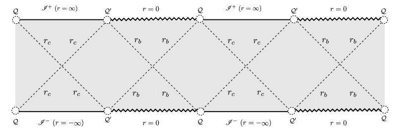
Figure 1: Penrose diagram of the sub-extremal Schwarzschild-de Sitter spacetime. The serrated line denotes the location of the singularity; the continuous black line denotes the conformal boundary; the dashed line shows the location of the black hole and Cosmological horizons denoted by $\mathcal{H}_{b}$ and $\mathcal{H}_{c}$ respectively. As described in the main text, these horizons are located at $r=r_{b}$ and $r=r_{c}$. The excluded points $\mathcal{Q}$ and $\mathcal{Q^{\prime}}$ where the singularity seems to meet the conformal boundary correspond to asymptotic regions of the spacetime that does not belong to the singularity nor the conformal boundary.

3.3 Other coordinate systems

In our analysis, we will also make use of retarded and advanced Eddington-Finkelstein null coordinates defined by

$$u\equiv t-r^{*},\qquad v\equiv t+r^{*},$$ (26)

where $r^{*}$ is the tortoise coordinate given by

$$r^{*}(t)\equiv\int\frac{\mathrm{d}r}{D(r)},\qquad\lim_{r\rightarrow\infty}r^{*}(r)=0.$$ (27)

It follows that $u,\,v\in\mathbb{R}$. In terms of these coordinates the metric $\mathring{\tilde{{\bm{g}}}}$ takes, respectively, the forms

$$\mathring{\tilde{{\bm{g}}}}=-D(r)\mathbf{d}u\otimes\mathbf{d}u+(\mathbf{d}u\otimes\mathbf{d}r+\mathbf{d}r\otimes\mathbf{d}u)+r^{2}{\bm{\sigma}},$$

$$\mathring{\tilde{{\bm{g}}}}=-D(r)\mathbf{d}v\otimes\mathbf{d}v+(\mathbf{d}v\otimes\mathbf{d}r+\mathbf{d}r\otimes\mathbf{d}v)+r^{2}{\bm{\sigma}}.$$

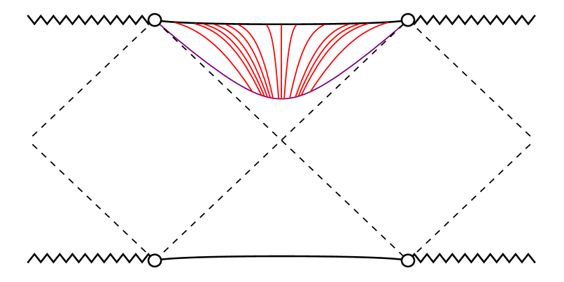
Figure 3: The conformal geodesics are plotted on the Penrose diagram of the Cosmological region of the sub-extremal Schwarzschild-de Sitter spacetime. The purple line represents the initial hypersurface $\mathcal{S}_{\star}$ corresponding to $r=r_{\star}$. The red lines represent conformal geodesics with constant time leaving this initial hypersurface. The curves are computed by setting $\lambda=3$ and $\phi=\frac{\pi}{4}$.

In order to compute the Penrose diagrams, Figures 2 and 3, we make use of Kruskal coordinates defined via

$$U\equiv\frac{1}{2}\exp(bu),\qquad V\equiv\frac{1}{2}\exp(bv)$$

where $u$ and $v$ are the Eddington-Finkelstein coordinates as defined in (26) and $b$ is a constant which can be freely chosen. A further change of coordinates is provided by

$$T\equiv U+V,\qquad\Psi\equiv U-V.$$

These coordinates are related to $r$ and $t$ via

$$T(r,t)=\cosh(bt)\exp(br^{*}(r)),\qquad\Psi(r,t)=\sinh(bt)\exp(br^{*}(r)).$$

Then by recalling that

$$r_{-}<0<r_{b}<r_{c}\qquad{\rm and}\qquad r_{-}+r_{b}+r_{c}=0,$$

the equation of $r^{*}(r)$ as defined by (27) renders

$$r^{*}(r)=-\frac{r_{b}\ln(r-r_{b})}{(r_{b}-r_{c})(2r_{b}+r_{c})}+\frac{r_{c}\ln(r-r_{c})}{r_{b}^{2}+r_{b}r_{c}-2r_{c}^{2}}+\frac{(r_{b}+r_{c})\ln(r+r_{b}+r_{c})}{(2r_{b}+r_{c})(r_{b}+2r_{c})}.$$

Hence, in order to have coordinates which are regular down to the Cosmological horizon, the constant $b$ must be given by

$$b=\frac{r_{b}^{2}+r_{b}r_{c}-2r_{c}^{2}}{2r_{c}}.$$

4 Construction of a conformal Gaussian gauge in the Cosmological region

The hyperbolic reduction of the extended conformal Einstein field equations to be used in this article makes use of a conformal Gaussian gauge system —i.e. coordinates and frame are propagated along a suitable congruence of conformal geodesics. This congruence provides, in turn, a canonical representative of the conformal class of a solution to the Einstein field equations —see e.g. Proposition 5.1 in [27].

A class of non-intersecting conformal geodesics which cover the whole maximal extension of the sub-extremal Schwarzschild-de Sitter spacetime has been studied in [12]. The main outcome of the analysis in that reference is that the resulting congruence covers the whole maximal analytic extension of the spacetime and, accordingly, provides a global system of coordinates —modulo the usual difficulties with the prescription of coordinates on $\mathbb{S}^{2}$. This congruence is prescribed in terms of data prescribed on a Cauchy hypersurface of the spacetime. In the present article, we are interested in the evolution of perturbations of the Schwarzschild-de Sitter spacetime from data prescribed on hypersurfaces of constant coordinate $r$ in the Cosmological region of the spacetime. Thus, the congruence of conformal geodesics constructed in [12] is of no direct use to us. Consequently, in this section, we study a class of conformal geodesics of the Schwarzschild-de Sitter spacetime which is prescribed in terms of data on hypersurfaces of constant $r$ in the Cosmological region. These curves turn out to be geodesics of the physical metric $\tilde{{\bm{g}}}$ and intersect the conformal boundary orthogonally.

4.1 Basic setup

In the following, it is assumed that

$$r_{c}<r<\infty$$

corresponding to the Cosmological region of the Schwarzschild-de Sitter spacetime. Given a fixed $r=r_{\star}$ we denote by $\mathcal{S}_{r_{\star}}$ (or $\mathcal{S}_{\star}$ for short) the spacelike hypersurfaces of constant $r=r_{\star}$ in this region —see Figure 2. Points on $\mathcal{S}_{\star}$ can be described in terms of the coordinates $(t,\theta,\varphi)$.

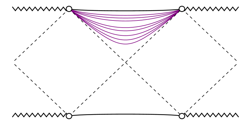
Figure 2: Hypersurfaces with constant $r$ are plotted on the Penrose diagram of the Cosmological region of the sub-extremal Schwarzschild-de Sitter spacetime.

4.1.1 Initial data for the congruence

In order to prescribe the congruence of conformal geodesics, we follow the general strategy outlined in [10, 12]. This requires prescribing the value of a conformal factor $\Theta_{\star}$ over $\mathcal{S}_{\star}$. We will only be interested on prescribing the data on compact subsets of $\mathcal{S}_{\star}$ so it is natural to require that

$$\Theta_{\star}=1,\qquad\dot{\Theta}_{\star}=0.$$

The second condition implies that the resulting conformal factor will have a time reflection symmetry with respect to $\mathcal{S}_{\star}$. Now, following [10, 12] we require that

$$\tilde{{\bm{x}}}^{\prime}_{\star}\perp\mathcal{S}_{\star},\qquad\tilde{\beta}_{\star}=\Theta_{\star}^{-1}{\rm d}\Theta_{\star}.$$

The latter, in turn, implies that

$$t=t_{\star}\qquad t{}^{\prime}{}_{\star}=\frac{1}{\sqrt{D_{\star}}},\qquad r{}^{\prime}{}_{\star}=0,\qquad\tilde{\beta}_{t\star}=0,\qquad\tilde{\beta}_{r\star}=0,$$ (28)

where $t_{\star}\in(-t_{\bullet},t_{\bullet})$ for some $t_{\bullet}\in\mathbb{R}^{+}$. Notice that the tangent vector $\tilde{x}^{\prime}$ coincides with the future unit normal to $\tilde{\mathcal{S}}$.

Given a sufficiently large constant $t_{\bullet}$ we define

$$\mathcal{R}_{\bullet}=\{p\in\mathcal{S}_{\star}\;|\;t(p)\in(-t_{\bullet},t_{\bullet})\}.$$

The constant $t_{\bullet}$ will be assumed to be large enough so that $D^{+}(\mathcal{R}_{\bullet})\cap\mathscr{I}^{+}\neq\varnothing$.

Remark 2.

The starting point of the curves on $\mathcal{S}_{\star}$ is prescribed in terms of the coordinates $(t,\theta,\varphi)=(t_{\star},\theta_{\star},\varphi_{\star})$ The conditions (28) gives rise to a congruence of conformal geodesics which has a trivial behaviour of the angular coordinates —that is, it is spherically symmetric. In other words effectively analysing the curves on a $2$-dimensional manifold $\tilde{\mathcal{M}}/{\rm SO}(3)$ with quotient metric $\tilde{{\bm{\ell}}}$ given by

$$\tilde{{\bm{\ell}}}=-D(r)\mathbf{d}t\otimes\mathbf{d}t+D^{-1}(r)\mathbf{d}r\otimes\mathbf{d}r$$

Accordingly, the only non-trivial parameter characterising each curve of the congruence is $t_{\star}$.

4.1.2 The geodesic equations

It follows that for the initial data conditions (28) one has $\beta^{2}=0$ so that the resulting congruence of conformal geodesics is, after reparametrisation, a congruence of metric geodesics. This last observation simplifies the subsequent discussion. The geodesic equations then imply that

$$r^{\prime}=\sqrt{\gamma^{2}-D(r)},\qquad D(r)t^{\prime}{}^{2}-\frac{1}{D(r)}r^{\prime 2}=1,$$ (29)

where $\gamma$ is a constant. Evaluating at $\mathcal{S}_{\star}$ one readily finds that

$$t_{\star}^{\prime}=\frac{|\gamma|}{|D_{\star}|}.$$

Observe that since we are in the Cosmological region of the spacetime we have that $D_{\star}<0$. Moreover, the unit normal to $\mathcal{S}_{\star}$ is given by

$${\bm{n}}=\bigg{(}\frac{1}{\sqrt{|D_{\star}|}}\bigg{)}\mathbf{d}r$$

while

$$\tilde{{\bm{x}}}^{\prime}{}_{\star}=\tilde{r}^{\prime}{}_{\star}{\bm{\partial}}_{r}+{t}^{\prime}{}_{\star}{\bm{\partial}}_{t}.$$

So, it follows that $\tilde{{\bm{x}}}_{\star}^{\prime}$ and ${\bm{n}}^{\sharp}$ are parallel if and only if $\gamma=0$.

4.1.3 The conformal factor

In the following, in order to obtain simpler expressions we set $\lambda=3$ and $\tau_{\star}=0$. It follows then from formula (13) that one gets an explicit expression for the conformal factor. Namely, one has that

$$\Theta(\tau)=1-\frac{1}{4}\tau^{2}.$$ (30)

The roots of $\Theta(\tau)$ are given by

$$\tau_{+}\equiv 2,\qquad\tau_{-}\equiv-2.$$

In the following, we concentrate on the root $\tau_{+}$ corresponding to the location of the future conformal boundary $\mathscr{I}^{+}$. The relation between the physical proper time $\tilde{\tau}$ and the unphysical proper time $\tau$ is obtained from equation (14) so that

$$\tilde{\tau}=2{\rm arctanh}\bigg{(}\frac{\tau}{2}\bigg{)},\qquad\tau=2{\rm tanh}\bigg{(}\frac{\tilde{\tau}}{2}\bigg{)}.$$ (31)

From these expressions, we deduce that

$$\tau\rightarrow\tau_{\pm}=2,\qquad\mbox{as}\quad\tilde{\tau}\rightarrow\infty.$$

Moreover, the conformal factor $\Theta$ can be rewritten in terms of the $\tilde{{\bm{g}}}$-proper time $\tilde{\tau}$ as

$$\Theta(\tilde{\tau})={\rm sech}^{2}\bigg{(}\frac{\tilde{\tau}}{2}\bigg{)}.$$

Remark 3.

In [11] it has been shown that conformal geodesics in an Einstein space will reach the conformal boundary orthogonally if and only if they are, up to a reparametrisation standard (metric) geodesics. In the present case, this property can be directly verified using equations (29).

4.2 Qualitative analysis of the behaviour of the curves

Having, in the previous subsection, set up the initial data for the congruence of conformal geodesics, in this subsection we analyse the qualitative behaviour of the curves. In particular, we show that the curves reach the conformal boundary in a finite amount of (conformal) proper time. Moreover, we also show that the curves do not intersect in the future of the initial hypersurface $\mathcal{S}_{\star}$.

4.2.1 Behaviour towards the conformal boundary

Recalling that

$$r^{\prime}=\sqrt{|D(r)|}$$ (32)

and observing that $D(r)<0$, it follows that if $r^{\prime}{}_{\star}\neq 0$ then, in fact $r^{\prime}>0$. Moreover, one can show that $r^{\prime\prime}{}_{\star}>0$ and that $r^{\prime\prime}{}_{\star}\neq 0$ for $r\in[r_{\star},\infty)$. Thus, the curves escape to the conformal boundary.

Now, we show that the congruence of conformal geodesics reaches the conformal boundary in an infinite amount of the physical proper time. In order to see this, we observe that $D(r)<0$, consequently from equation

$$r^{\prime}=\pm\sqrt{|D(r)|}$$

it follows that $r(\tilde{\tau})$ is a monotonic function. Moreover, using equations

$$D(r)=-\frac{1}{r}(r-r_{b})(r-r_{-})(r-r_{c})$$

and

$$t^{\prime}=\frac{|\gamma+\beta r|}{|D(r)|}=0$$

we find that

$$\tilde{\tau}=\bigintss_{r_{\star}}^{r}\sqrt{\frac{\bar{r}}{(\bar{r}-r_{b})(\bar{r}-r_{c})(\bar{r}-r_{-})}}{\rm d}\bar{r}.$$

It is possible to rewrite this integral in terms of elliptic functions —see e.g. [19]. More precisely, one has that

$$\tilde{\tau}=\frac{2r_{\star}}{\alpha^{2}\sqrt{r_{\star}(\alpha_{+}-\alpha_{-})}}\bigg{(}\kappa^{2}{\rm w}+(\alpha^{2}-\kappa^{2})\Pi[\phi,\alpha^{2},\kappa]\bigg{)},$$ (33)

where $\Pi[\phi,\alpha^{2},\kappa]$ is the incomplete elliptic integral of the third kind and

$${\rm sn}^{2}{\rm w}=\bigg{(}\frac{r_{c}-r_{-}}{r_{b}-r_{-}}\bigg{)}\bigg{(}\frac{r-r_{b}}{r-r_{c}}\bigg{)},\qquad\alpha^{2}\equiv\frac{r_{b}-r_{-}}{r_{c}-r_{-}},$$

$$\kappa^{2}\equiv\frac{r_{c}(r_{b}-r_{-})}{r_{\star}(r_{c}-r_{-})},\qquad\phi\equiv{\rm arcsin}({\rm sn}{\rm w}),$$

with $\mathrm{sn}$ denotes the Jacobian elliptic function. From the previous expressions and the general theory of elliptic functions it follows that $\tilde{\tau}(r,r_{\star})$ as defined by Equation (33) is an analytic function of its arguments. Moreover, it can be verified that

$$\tilde{\tau}\rightarrow\infty\qquad\mbox{as}\quad r\rightarrow\infty.$$

Accordingly, as expected, the curves escape to infinity in an infinite amount of physical proper time. Using the reparametrisation formulae (31) the latter corresponds to a finite amount of unphysical proper time.

4.2.2 Analysis of the behaviour of the conformal deviation equation

In [10] (see also [12]) it has been shown that for congruences of conformal geodesics in spherically symmetric spacetimes the behaviour of the deviation vector of the congruence can be understood by considering the evolution of a scalar $\tilde{\omega}$ —see equation (33) in [12]. If this scalar does not vanish, then the congruence is non-intersecting. Since in the present case one has $\beta=0$, it follows that the evolution equation for $\tilde{\omega}$ takes the form

$$\frac{{\rm d}^{2}\tilde{\omega}}{{\rm d}\tilde{\tau}^{2}}=\bigg{(}1+\frac{M}{r^{3}}\bigg{)}\tilde{\omega},\qquad r\equiv r(\tilde{\tau},r_{\star}).$$

Since in our setting $r\geq r_{\star}>r_{c}$, it follows that

$$1+\frac{M}{r^{3}}>1,$$

from where, in turn, one obtains the inequality

$$\frac{{\rm d}^{2}\tilde{\omega}}{{\rm d}\tilde{\tau}^{2}}>\tilde{\omega}.$$

Accordingly, the scalars $\tilde{\omega}$ and $\omega\equiv\Theta\tilde{\omega}$ satisfy the inequalities

$$\tilde{\omega}\geq\bar{\omega},\qquad\omega\geq\Theta\bar{\omega},$$

where $\bar{\omega}$ is the solution of

$$\frac{{\rm d}^{2}\bar{\omega}}{{\rm d}\tilde{\tau}^{2}}=\bar{\omega},\qquad\bar{\omega}(0,\rho_{\star})=\frac{r_{\star}}{\rho_{\star}},\qquad\bar{\omega}^{\prime}(0,\rho_{\star})=0.$$

The solution to this last differential equation is given by

$$\bar{\omega}=(r_{\star}/\rho_{\star}){\rm cosh}\tilde{\tau}.$$

Using equations (30) and (31) we get the inequality

$$\omega\geq\bigg{(}1-\frac{\tau^{2}}{4}\bigg{)}\frac{r_{\star}}{\rho_{\star}}{\rm cosh}\bigg{(}2{\rm arctanh}\bigg{(}\frac{\tau}{2}\bigg{)}\bigg{)}=\frac{r_{\star}}{\rho_{\star}}\bigg{(}1+\frac{\tau^{2}}{4}\bigg{)}>0.$$

Consequently, we get the limit

$$\lim_{\tau\to\pm 2}\omega\geq\frac{2r_{\star}}{\rho_{\star}}>0.$$

Hence, we conclude that the geodesics with $r_{\star}>r_{\bullet}$ which go to the conformal boundary $\mathscr{I}^{+}$ located at $\tau=2$ do not develop any caustics.

The discussion of the previous paragraphs can be summarised in the following:

Proposition 1.

The congruence of conformal geodesics given by the initial conditions (28) leaving the initial hypersurface $\mathcal{S}_{\star}$ reach the conformal boundary $\mathscr{I}^{+}$ without developing caustics.

The content of this Proposition can be visualised in Figure [3].

4.3 Estimating the size of $D^{+}(\mathcal{R}_{\bullet})$

Up to this point the size of the domain $\mathcal{R}_{\bullet}\subset\mathcal{S}_{\star}$ (or more precisely, the value of the constant $t_{\bullet}$ has remained unspecified). An inspection of the Penrose diagram of the Schwarzschild-de Sitter spacetime shows that if the value of $t_{\bullet}$ is too small, it could happen that the future domain of dependence $D^{+}(\mathcal{R}_{\bullet})$ is bounded and, accordingly, will not reach the spacelike conformal boundary $\mathscr{I}^{+}$ —see e.g. Figure 4. Given our interest in constructing perturbations of the Schwarzschild-de Sitter spacetime which contain as much as possible of the conformal boundary it is then necessary to ensure that $t_{\bullet}$ is sufficiently large. In this subsection given a fiduciary hypersurface $\mathcal{S}_{\star}$ in the Cosmological region of the spacetime, we provide an estimate of how large should $t_{\bullet}$ be for $D^{+}(\mathcal{R}_{\bullet})$ to be unbounded. In order to obtain this estimate we consider the future-oriented inward-pointing null geodesics emanating from the end-points of $\mathcal{R}_{\bullet}$ and look at where these curves intersect the conformal boundary.

In order to carry out the analysis in this subsection it is convenient to consider the coordinate $z\equiv 1/r$. In terms of this new coordinate, the line element (23) takes the form

$$\mathring{\tilde{{\bm{g}}}}=\frac{1}{z^{2}}\bigg{(}-F(z)\mathbf{d}t\otimes\mathbf{d}t+\frac{1}{F(z)}\mathbf{d}z\otimes\mathbf{d}z+\bm{\sigma}\bigg{)},$$

where

$$F(z)\equiv z^{2}D(1/z).$$

The above expression suggest defining an unphysical metric $\bar{{\bm{g}}}$ via

$$\bar{{\bm{g}}}=\Xi^{2}\mathring{\tilde{{\bm{g}}}},\qquad\Xi\equiv z.$$

More precisely, one has

$$\bar{{\bm{g}}}=-F(z)\mathbf{d}t\otimes\mathbf{d}t+\frac{1}{F(z)}\mathbf{d}z\otimes\mathbf{d}z+\bm{\sigma}.$$ (34)

In order to study the null geodesics we consider the Lagrangian

$$\mathcal{L}=-F(z)\dot{t}^{2}+\frac{1}{F(z)}\dot{z}^{2},$$

where $\cdot\equiv\frac{d}{ds}$. In the case of null conformal geodesics $\mathcal{L}=0$ so that

$$\dot{t}=\pm\frac{1}{F(z)}\dot{z}.$$

This, in turn, means that

$$\frac{dt}{dz}\dot{z}=\pm\frac{1}{F(z)}\dot{z}.$$

By integrating both sides it follows that

$$\int_{t_{\bullet}}^{t_{+}}dt=\pm\int_{z_{\star}}^{0}\frac{1}{F(z)}dz,$$

where $t_{+}$ denotes the value of the (spacelike) coordinate $t$ at which the null geodesic reaches $\mathscr{I}^{+}$. Accordingly for the inward-pointing light rays emanating from the points on $\mathcal{S}_{\star}$ defined by the condition $t=t_{\bullet}$ one has that

$$t_{+}=t_{\bullet}-\int_{0}^{z_{\star}}\frac{1}{F(z)}dz.$$ (35)

An analogous condition holds for the inward-pointing light rays emanating from the points with $t=-t_{\bullet}$. Since in the Cosmological region $F(z)>0$ it follows that

$$\int_{0}^{z_{\star}}\frac{1}{F(z)}dz>0.$$

The key observation in the analysis in this subsection is the following: $D^{+}(\mathcal{R}_{\bullet})$ is unbounded (so that it intersects the conformal boundary) if $t_{+}$ as given by equation (35) satisfies $t_{+}>0$. As $t_{\bullet}>0$, having $t_{+}<0$ would mean that the light rays emanating from the points with $t=t_{\bullet}$ and $t=-t_{\bullet}$ intersect before reaching $\mathscr{I}^{+}$. Now, the condition $t_{+}>0$ implies, in turn, that

$$t_{\bullet}>\int_{0}^{z_{\star}}\frac{1}{F(z)}dz.$$

As the integral in the right-hand side of the above inequality is not easy to compute we provide, instead, a lower bound. One has then that

$$t_{\bullet}>\frac{z_{\star}}{F_{\circledast}},$$

where $F_{\circledast}$ denotes the maximum of

$$F(z)=z^{2}-Mz^{3}+1$$

over the interval $[0,z_{\star}]$. Thus, $F^{\prime}(z)$ vanishes if $z=0$ or $z=z_{\odot}\equiv 2/3M$. Also, notice that $F^{\prime}(z)>0$ for $z\approx 0$. It can be readily verified that $F^{\prime\prime}(0)>0$ while $F^{\prime\prime}(2/3M)<0$ so that an inflexion point occurs in the interval $(0,z_{\odot})$ and there are no other inflexion points in $[0,z_{\star}]$. Now, looking at the definition of $M$, equation (24c), and the expression for $r_{c}$ as given by equation (25) one concludes that $z_{\odot}>z_{c}\equiv 1/r_{c}$. As $z_{\odot}$ is independent of $z_{\star}$, it is not possible to decide whether $z_{\odot}$ lies in $[0,z_{\star}]$ or not. In any case, one has that

$$F(z_{\odot})=1+\frac{4}{27M^{2}}\geq F_{\circledast},$$

so that

$$t_{\bullet}>\frac{27M^{2}z_{\star}}{27M^{2}+4}.$$ (36)

One can summarise the discussion in this subsection as follows:

Lemma 3.

If condition (36) holds then $D^{+}(\mathcal{R}_{\bullet})$ is unbounded.

Remark 4.

In the rest of this article it is assumed that condition (36) always holds.

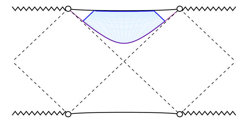
Figure 4: The plotted future domain of dependence of the solution $D^{+}(\mathcal{R}_{\bullet})$ on the Penrose diagram of the Cosmological region of the sub-extremal Schwarzschild-de Sitter spacetime. The value of $t_{\bullet}$ can be chosen as close as possible to the asymptotic points $\mathcal{Q}$ and $\mathcal{Q}^{\prime}$ so as to satisfy condition (36).

4.4 Conformal Gaussian coordinates in the sub-extremal Schwarzschild-de Sitter spacetime

We now combine the results of the previous subsections to show that the congruence of conformal geodesics defined by the initial conditions (28) can be used to construct a conformal Gaussian coordinate system in a domain in the chronological future of $\mathcal{R}_{\bullet}\subset\mathcal{S}_{\star}$, $J^{+}(\mathcal{R}_{\bullet}\subset\mathcal{S}_{\star})$, containing a portion of the conformal boundary $\mathscr{I}^{+}$.

In the following let $\widetilde{SdS}_{I}$ denote the Cosmological region of the Schwarzschild-de Sitter spacetime —that is

$$\widetilde{SdS}_{I}=\{p\in\tilde{\mathcal{M}}\;|\;r(p)>r_{c}\}.$$

Moreover, denote by $SdS_{I}$ the conformal representation of $\widetilde{SdS}_{I}$ defined by the conformal factor $\Theta$ defined by the non-singular congruence of conformal geodesics given by Proposition 1. For $r>r_{c}$ let $z\equiv 1/r$ —cfr the line element (34). In terms of these coordinates, one has that

$$SdS_{I}=\{p\in\mathbb{R}\times\mathbb{R}\times\mathbb{S}^{2}\;|\;0\leq z(p)\leq z_{\star}\}$$ (37)

where $z_{\star}\equiv 1/r_{\star}$ with $r_{\star}>r_{c}$. In particular, the conformal boundary, $\mathscr{I}^{+}$, corresponds to the set of points for which $z=0$.

The analysis of the previous subsections shows that the conformal geodesics defined by the initial conditions (28) can be thought of as curves on $SdS_{I}$ of the form

$$(\tau,t_{\star})\mapsto\big{(}t(\tau,t_{\star}),z(\tau,t_{\star}),\theta_{\star},\varphi_{\star}\big{)}.$$

Thus, in particular, the congruence of curves defines a map

$$\psi:[0,2]\times[-t_{\bullet},t_{\bullet}]\rightarrow[0,z_{\star}]\times[-t_{\bullet},t_{\bullet}].$$

This map is analytic in the parameters $(\tau,t_{\star})$. Moreover, the fact that the congruence of conformal geodesics is non-intersecting implies that the map is, in fact, invertible —the analysis of the conformal geodesic deviation equation implies that the Jacobian of the transformation is non-zero for the given value of the parameters. In particular, it can be readily verified that the function $\Theta\tilde{\omega}$ coincides with the Jacobian of the transformation. Accordingly, the inverse map $\psi^{-1}$

$$\psi^{-1}:[0,z_{\star}]\times[-t_{\bullet},t_{\bullet}]\rightarrow[0,2]\times[-t_{\bullet},t_{\bullet}],\qquad(t,z)\mapsto\big{(}\tau(t,z),t_{\star}(t,z)\big{)}$$

is well-defined. Thus, $\psi^{-1}$ gives the transformation from the standard Schwarzschild coordinates $(t,z,\theta,\varphi)$ into the conformal Gaussian coordinates $(\tau,t_{\star},\theta,\varphi)$. In the following let

$$\mathcal{M}_{\bullet}\equiv[0,2]\times[-t_{\bullet},t_{\bullet}].$$

As the conformal geodesics of our congruence are timelike, we have that

$$\mathcal{M}_{\bullet}\subset J^{+}(\mathcal{R}_{\bullet}).$$

All throughout we assume, as discussed in Subsections 4.1.1 and 4.3, that $t_{\bullet}$ is sufficiently large to ensure that $D^{+}(\mathcal{R}_{\bullet})$ contains a portion of $\mathscr{I}^{+}$ —cfr Lemma 3.

Proposition 2.

The congruence of conformal geodesics on $SdS_{I}$ defined by the initial conditions on $\mathcal{S}_{\star}$ given by (28) induce a conformal Gaussian coordinate system over $D^{+}(\mathcal{R}_{\bullet})$ which is related to the standard coordinates $(t,r)$ via a map which is analytic.

5 The Schwarzschild-de Sitter spacetime in the conformal Gaussian system

In the previous section, we have established the existence of conformal Gaussian coordinates in the domain $\mathcal{M}_{\bullet}\subset SdS_{I}$ of the Schwarzschild-de Sitter spacetime. In this section, we proceed to analyse the properties of this exact solution in these coordinates. This analysis is focused on the structural properties relevant for the analysis of stability in the latter parts of this article.

Remark 5.

The metric coefficients implied by the line element (34) are analytic functions of the coordinates in the region $\mathcal{M}_{\bullet}$ —barring the usual degeneracy of spherical coordinates.

5.1 Weyl propagated frames

The ultimate aim of this section is to cast the Schwarzschild-de Sitter spacetime in the region $\mathcal{M}_{\bullet}$ as a solution to the extended conformal Einstein field equations introduced in Section 2.1.3. A key step in this construction is the use of a Weyl propagated frame. In this section, we discuss a class of these frames in $\mathcal{M}_{\bullet}$.

Since the congruence of conformal geodesics implied by the initial data (28) satisfies $\tilde{{\bm{\beta}}}=0$, the Weyl propagation equation (20) reduces to the usual parallel propagation equation —that is,

$$\tilde{\nabla}_{\tilde{{\bm{x}}}^{\prime}}(\Theta\tilde{{\bm{e}}}_{\bm{a}})=\tilde{\nabla}_{\tilde{{\bm{x}}}^{\prime}}{\bm{e}}_{\bm{a}}=0.$$ (38)

The subsequent computations can be simplified by noticing that the line element (23) is in warped-product form. Given the spherical symmetry of the Schwarzschild-de Sitter spacetime, most of the discussion of a frame adapted to the symmetry of the spacetime can be carried out by considering the 2-dimensional Lorentzian metric

$${\bm{\ell}}=\ell_{AB}\mathbf{d}x^{A}\otimes\mathbf{d}x^{B}$$

$$\phantom{{\bm{\ell}}}=-D(r)\mathbf{d}t\otimes\mathbf{d}t+\frac{1}{D(r)}\mathbf{d}r\otimes\mathbf{d}r.$$

In the spirit of a conformal Gaussian system, we begin by setting the time leg of the frame as ${\bm{e}}_{\bm{0}}=\dot{{\bm{x}}}$. Then since

$$\dot{{\bm{x}}}=\Theta^{-1}\tilde{{\bm{x}}}^{\prime},$$

it follows that

$${\bm{e}}_{\bm{0}}=\Theta^{-1}\tilde{{\bm{x}}}^{\prime}.$$

Now, recall that

$$\tilde{{\bm{x}}}^{\prime}=\tilde{t}^{\prime}{\bm{\partial}}_{t}+\tilde{r}^{\prime}{\bm{\partial}}_{r},\qquad\tilde{t}=t(\tilde{\tau}),\quad\tilde{r}=r(\tilde{\tau}),$$

and let

$${\bm{\omega}}\equiv\epsilon_{\bm{\ell}}(\tilde{{\bm{x}}}^{\prime},\cdot).$$

It follows then that $\langle{\bm{\omega}},\tilde{{\bm{x}}}^{\prime}\rangle=0$ so that it is natural to consider a radial leg of the frame, ${\bm{e}}_{\bm{1}}$, which is proportional to ${\bm{\omega}}^{\sharp}$. By using the condition ${\bm{\ell}}({\bm{e}}_{\bm{1}},{\bm{e}}_{\bm{1}})=1$ one readily finds that

$${\bm{e}}_{\bm{1}}=\Theta{\bm{\omega}}^{\sharp}.$$

It can be readily verified by a direct computation that the vector ${\bm{e}}_{\bm{1}}$ as defined above satisfies the propagation equation (38).

Finally, the vectors ${\bm{e}}_{\bm{2}}$ and ${\bm{e}}_{\bm{3}}$ are chosen in such a way that they span the tangent space of the 2-spheres associated to the orbits of the spherical symmetry. Accordingly, by setting

$${\bm{e}}_{\bm{2}}=e_{\bm{2}}{}^{\mathcal{A}}{\bm{\partial}}_{\mathcal{A}},\qquad{\bm{e}}_{\bm{3}}=e_{\bm{3}}{}^{\mathcal{A}}{\bm{\partial}}_{\mathcal{A}},\qquad\mathcal{A}=2,\,3,$$

it follows readily from the warped-product structure of the metric that

$$\tilde{x}^{\prime A}(\partial_{A}e_{{\bm{2}}}{}^{\mathcal{A}})=\tilde{x}^{\prime A}(\partial_{A}e_{{\bm{3}}}{}^{\mathcal{A}})=0.$$

In other words, one has that the frame coefficients $e_{{\bm{2}}}{}^{\mathcal{A}}$ and $e_{{\bm{3}}}{}^{\mathcal{A}}$ are constant along the conformal geodesics. Thus, in order to complete the Weyl propagated frame $\{{\bm{e}}_{\bm{a}}\}$ we choose two arbitrary orthonormal vectors $\tilde{{\bm{e}}}_{{\bm{2}}\star}$ and $\tilde{{\bm{e}}}_{{\bm{3}}\star}$ spanning the tangent space of $\mathbb{S}^{2}$ and define vectors $\{{\bm{e}}_{\bm{2}},{\bm{e}}_{\bm{3}}\}$ on $\mathcal{M}_{\bullet}$ by extending (constantly) the value of the associated coefficients $\big{(}e_{\bm{2}}{}^{\mathcal{A}}\big{)}_{\star}$ and $\big{(}e_{\bm{3}}{}^{\mathcal{A}}\big{)}_{\star}$ along the conformal geodesic.

The analysis of this subsection can be summarised in the following:

Proposition 3.

Let $\tilde{{\bm{x}}}^{\prime}$ denote the vector tangent to the conformal geodesics defined by the initial data (28) and let $\{{\bm{e}}_{{\bm{2}}\star},\,{\bm{e}}_{{\bm{3}}\star}\}$ be an arbitrary orthonormal pair of vectors spanning the tangent bundle of $\mathbb{S}^{2}$. Then the frame $\{{\bm{e}}_{\bm{0}},\,{\bm{e}}_{\bm{1}},\,{\bm{e}}_{\bm{2}},\,{\bm{e}}_{\bm{3}}\}$ obtained by the procedure described in the previous paragraphs is a ${\bm{g}}$-orthonormal Weyl propagated frame. The frame depends analytically on the unphysical proper time $\tau$ and the initial position $t_{\star}$ of the curve.

Remark 6.

In the previous proposition we ignore the usual complications due to the non-existence of a globally defined basis of $T\mathbb{S}^{2}$. The key observation is that any local choice works well.

5.2 The Weyl connection

The connection coefficients associated to a conformal Gaussian gauge are made up of two pieces: the 1-form defining the Weyl connection and the Levi-Civita connection of the metric $\bar{{\bm{g}}}$. We analyse these two pieces in turn.

5.2.1 The 1-form associated to the Weyl connection

We start by recalling that in Section 4 a congruence of conformal geodesics with data prescribed on the hypersurface $\mathcal{S}_{\star}$ was considered. This congruence was analysed using the $\tilde{{\bm{g}}}$-adapted conformal geodesic equations. The initial data for this congruence was chosen so that the curves with tangent given by $\tilde{{\bm{x}}}^{\prime}$ satisfy the standard (affine) geodesic equation. Consequently, the (spatial) 1-form $\tilde{{\bm{\beta}}}$ vanishes. Thus, the 1-form ${\bm{\beta}}$ is given by

$${\bm{\beta}}=-\dot{\Theta}\tilde{{\bm{x}}}^{\prime\flat},$$

—cfr. equation (16). Now, recalling that $\tilde{{\bm{x}}}^{\prime}=r^{\prime}{\bm{\partial}}_{r}$ and observing equation (32) one concludes that

$$\tilde{{\bm{x}}}^{\prime\flat}=\frac{1}{|\sqrt{D(r)}|}\mathbf{d}r.$$

Rewritten in terms of $z$, the latter gives

$$\tilde{{\bm{x}}}^{\prime\flat}=-\frac{1}{z\sqrt{|F(z)|}}\mathbf{d}z.$$

As $F(0)=1$, and $\dot{\Theta}|_{\mathscr{I}^{+}}=-1$ (cfr. equation (30)), it then follows that

$${\bm{\beta}}\approx-\frac{1}{z}\mathbf{d}z\qquad\mbox{for}\quad z\approx 0.$$

That is, ${\bm{\beta}}$ is singular at the conformal boundary. However, in the subsequent analysis the key object is not ${\bm{\beta}}$ but $\bar{{\bm{\beta}}}$, the 1-form associated to the conformal geodesics equations written in terms of the connection $\bar{{\bm{\nabla}}}$. Now, from the conformal transformation rule $\bar{{\bm{\beta}}}={\bm{\beta}}+\Xi^{-1}\mathbf{d}\Xi$ and recalling that $\Xi=z$ it follows that

$$\bar{{\bm{\beta}}}=\frac{\dot{\Theta}}{z\sqrt{|F(z)|}}\mathbf{d}z+\frac{1}{z}\mathbf{d}z.$$

Thus, from the preceding discussion it follows that $\bar{{\bm{\beta}}}$ is smooth at $\mathscr{I}^{+}$ and, moreover, $\bar{{\bm{\beta}}}|_{\mathscr{I}^{+}}=0$. Notice, however, that $\bar{{\bm{\beta}}}\neq 0$ away from the conformal boundary.

5.2.2 Computation of the connection coefficients

The 1-form ${\bm{\beta}}$ defines in a natural way a Weyl connection $\hat{{\bm{\nabla}}}$ via the relation

$$\hat{{\bm{\nabla}}}-\tilde{{\bm{\nabla}}}=\mathbf{S}({\bm{\beta}})$$

where $\mathbf{S}$ corresponds to the tensor $S_{ab}{}^{cd}$ as defined in (3). As the coordinates and connection coefficients associated to the physical connection $\tilde{{\bm{\nabla}}}$ are not well adapted to a discussion near the conformal boundary we resort to the unphysical Levi-Civita connection $\bar{{\bm{\nabla}}}$ to compute $\hat{{\bm{\nabla}}}$. From the discussion in the previous subsections, we have that

$$\bar{{\bm{\nabla}}}-\tilde{{\bm{\nabla}}}=\mathbf{S}(z^{-1}\mathbf{d}z).$$

It thus follows that

$$\hat{{\bm{\nabla}}}-\bar{{\bm{\nabla}}}=\mathbf{S}(\bar{{\bm{\beta}}}).$$

Now let $\{{\bm{e}}_{\bm{a}}\}$ denote the Weyl propagated frame as given by Proposition 3. The connection coefficients $\hat{\Gamma}_{\bm{a}}{}^{\bm{b}}{}_{\bm{c}}$ are defined through the relation

$$\hat{\nabla}_{\bm{a}}{\bm{e}}_{\bm{c}}=\hat{\Gamma}_{\bm{a}}{}^{\bm{b}}{}_{\bm{c}}{\bm{e}}_{\bm{b}}.$$

Now, writing ${\bm{e}}_{\bm{a}}=e_{\bm{a}}{}^{\mu}{\bm{\partial}}_{\mu}$ one has that

$$\hat{\nabla}_{\bm{a}}{\bm{e}}_{\bm{c}}=\big{(}\hat{\nabla}_{\mu}e_{\bm{c}}{}^{\nu}\big{)}e_{\bm{a}}{}^{\mu}{\bm{\partial}}_{\nu},$$

where

$$\hat{\nabla}_{\mu}e_{\bm{c}}{}^{\nu}=\bar{\nabla}_{\mu}e_{\bm{c}}{}^{\nu}+S_{\mu\lambda}{}^{\nu\rho}\bar{\beta}_{\rho}e_{\bm{c}}{}^{\lambda},$$

$$\phantom{\hat{\nabla}_{\mu}e_{\bm{c}}{}^{\nu}}=\partial_{\mu}e_{\bm{c}}{}^{\nu}+\bar{\Gamma}_{\mu}{}^{\nu}{}_{\lambda}e_{\bm{c}}{}^{\lambda}+S_{\mu\lambda}{}^{\mu\rho}\bar{\beta}_{\rho}e_{\bm{c}}{}^{\lambda}.$$ (39)

A direct computation shows that the only non-vanishing Christoffel symbols of the metric (34), $\bar{\Gamma}_{\mu}{}^{\nu}{}_{\lambda}$ are given by

$$\bar{\Gamma}_{t}{}^{t}{}_{z}=-\bar{\Gamma}_{z}{}^{z}{}_{z}=\frac{z(\frac{3}{2}Mz-1)}{1+z^{2}(Mz-1)},$$

$$\bar{\Gamma}_{t}{}^{z}{}_{t}=z(\tfrac{3}{2}Mz-1)\big{(}1+z^{2}(Mz-1)\big{)},$$

$$\bar{\Gamma}_{\varphi}{}^{\theta}{}_{\varphi}=-\cos\theta\sin\theta,\qquad\bar{\Gamma}_{\theta}{}^{\varphi}{}_{\varphi}=\cot\theta.$$

Observe that the coefficients $\bar{\Gamma}_{t}{}^{t}{}_{z}$, $\bar{\Gamma}_{z}{}^{z}{}_{z}$ and $\bar{\Gamma}_{t}{}^{z}{}_{t}$ are analytic at $z=0$.

Remark 7.

The connection coefficients $\bar{\Gamma}_{\varphi}{}^{\theta}{}_{\varphi}$, $\bar{\Gamma}_{\theta}{}^{\varphi}{}_{\varphi}$ correspond to the connection of the round metric over $\mathbb{S}^{2}$. In the rest of this section, we ignore this coordinate singularity due to the use of spherical coordinates.

It follows from the discussion in the previous paragraphs and Proposition 3 that each of the terms in the righthand side of (39) is a regular function of the coordinate $z$ and, in particular, analytic at $z=0$. Contraction with the coefficients of the frame does not change this. Accordingly, it follows that the Weyl connection coefficients $\hat{\Gamma}_{\bm{a}}{}^{\bm{b}}{}_{\bm{c}}$ are smooth functions of the coordinates used in the conformal Gaussian gauge on the future of the fiduciary initial hypersurface $\mathcal{S}_{\star}$ up to and beyond the conformal boundary.

5.3 The components of the curvature

In this section we discuss the behaviour of the various components of the curvature of the Schwarzschild-de Sitter spacetime in the domain $\mathcal{M}_{\bullet}$. We are particularly interested in the behaviour of the curvature at the conformal boundary.

The subsequent discussion is best done in terms of the conformal metric $\bar{{\bm{g}}}$ as given by (34). Consider also the vector $\bar{{\bm{e}}}_{\bm{0}}$ given by

$$\bar{{\bm{e}}}_{\bm{0}}=\sqrt{|F(z)|}{\bm{\partial}}_{z},\qquad F(z)=z^{2}-Mz^{3}-1.$$

This vector is orthogonal to the conformal boundary $\mathscr{I}^{+}$ which, in these coordinates is given by the condition $z=0$.

5.3.1 The rescaled Weyl tensor

Given a timelike vector, the components of the rescaled Weyl tensor $d_{abcd}$ can be conveniently encoded in the electric and magnetic parts relative to the given vector. For the vector $\bar{{\bm{e}}}_{\bm{0}}$ these are given by

$$d_{ac}=d_{abcd}\bar{e}_{\bm{0}}{}^{b}\bar{e}_{\bm{0}}{}^{d},\qquad d^{*}{}_{ac}=d{}^{*}{}_{abcd}\bar{e}_{{\bm{0}}}{}^{b}\bar{e}_{\bm{0}}{}^{d},$$

where $d{}^{*}{}_{abcd}$ denotes the Hodge dual of $d_{abcd}$. A computation using the package xAct for Mathematica readily gives that the only non-zero components of the electric part are given by

$$d_{tt}=-M\big{(}z^{2}(1-Mz)-1\big{)},$$

$$d_{\theta\theta}=-\frac{M}{2},$$

$$d_{\varphi\varphi}=-\frac{M}{2}\sin^{2}\theta,$$

while the magnetic part vanishes identically. Observe, in particular, that the above expressions are regular at $z=0$ —again, disregarding the coordinate singularity due to the use of spherical coordinates. The smoothness of the components of the Weyl tensor is retained when re-expressed in terms of the Weyl propagated frame $\{{\bm{e}}_{\bm{a}}\}$ as given in Proposition 3.

5.3.2 The Schouten tensor

A similar computer algebra calculation shows that the non-zero components of the Schouten tensor of the metric $\bar{{\bm{g}}}$ are given by

$$\bar{L}_{tt}=\frac{1}{2}(2Mz-1)(1+z^{2}(Mz-1)),$$

$$\bar{L}_{zz}=-\frac{1}{2}\frac{(2Mz-1)}{1+z^{2}(Mz-1)},$$

$$\bar{L}_{\theta\theta}=-\frac{1}{2}(Mz-1),$$

$$\bar{L}_{\varphi\varphi}=-\frac{1}{2}\sin^{2}\theta(Mz-1).$$

Again, disregarding the coordinate singularity on the angular components, the above expressions are analytic on $\mathcal{M}_{\bullet}$ —in particular at $z=0$. To obtain the components of the Schouten tensor associated to the Weyl connection $\hat{\nabla}$ we make use of the transformation rule

$$\bar{L}_{ab}-\hat{L}_{ab}=\bar{\nabla}_{a}\bar{\beta}_{b}-\frac{1}{2}S_{ab}{}^{cd}\bar{\beta}_{c}\bar{\beta}_{d}.$$

The smoothness of $\bar{\beta}_{a}$ has already been established in Subsection 5.2. It follows then that the components of $\hat{L}_{ab}$ with respect to the Weyl propagated frame $\{{\bm{e}}_{\bm{a}}\}$ are regular on $\mathcal{M}_{\bullet}$.

5.4 Summary

The analysis of the preceding subsections is summarised in the following:

Proposition 4.

Given $t_{\bullet}>0$ and the Weyl propagated frame $\{{\bm{e}}_{\bm{a}}\}$ as given by Proposition 3, the connection coefficients of the Weyl connection associated to the congruence of conformal geodesics, the components of the rescaled Weyl tensor and the components of the Schouten tensor of the Weyl connection are smooth on $\mathcal{M}_{\bullet}$ and, in particular, at the conformal boundary.

Remark 8.

In other words, the sub-extremal Schwarzschild-de Sitter spacetime expressed in terms of a conformal Gaussian gauge system gives rise to a solution to the extended conformal Einstein field equations on the region $\mathcal{M}_{\bullet}\subset D^{+}(\mathcal{R}_{\bullet})$ where $\mathcal{R}_{\bullet}\subset\mathcal{S}_{\star}$.

5.5 Construction of a background solution with compact spatial sections

The region $\mathcal{R}_{\bullet}\subset\mathcal{S}_{\star}$ has the topology of $I\times\mathbb{S}^{2}$ where $I\subset\mathbb{R}$ is an open interval. Accordingly, the spacetime arising from $\mathcal{R}_{\bullet}$ will have spatial sections with the same topology. As part of the perturbative argument given in Section 6 based on the general theory of symmetric hyperbolic systems as given in [18] it is convenient to consider solutions with compact spatial sections. We briefly discuss how the (conformal) Schwarzschild-de Sitter spacetime in the conformal Gaussian system over $\mathcal{M}_{\bullet}$ can be recast as a solution to the extended conformal Einstein field equations with compact spatial sections.

The key observation on this construction is that the Killing vector ${\bm{\xi}}={\bm{\partial}}_{t}$ in the Cosmological region of the spacetime is spacelike. Thus, given a fixed $z_{\circ}<z_{c}$, we have that the hypersurface $\mathcal{S}_{z_{\circ}}$ defined by the condition $z=z_{\circ}$ has a translational invariance —that is, the intrinsic metric ${\bm{h}}$ and the extrinsic curvature ${\bm{K}}$ are invariant under the replacement $t\mapsto t+\varkappa$ for $\varkappa\in\mathbb{R}$. Moreover, the congruence of conformal geodesics given by Proposition 4 are such that the value of the coordinate $t$ is constant along a given curve.

Consider now, the timelike hypersurfaces $\mathcal{T}_{-2t_{\bullet}}$ and $\mathcal{T}_{2t_{\bullet}}$ in $D^{+}(\mathcal{S}_{\star})$ generated, respectively, by the future-directed geodesics emanating from $\mathcal{S}_{\star}$ at the points with $t=-2t_{\bullet}$ and $t=2t_{\bullet}$. From the discussion in the previous paragraph, one can identify $\mathcal{T}_{-2t_{\bullet}}$ and $\mathcal{T}_{2t_{\bullet}}$ to obtain a smooth spacetime manifold $\bar{\mathcal{M}}_{\bullet}$ with compact spatial sections —see Figure 5. A natural foliation of $\bar{\mathcal{M}}_{\bullet}$ is given by the hypersurfaces $\bar{\mathcal{S}}_{z}$ of constant $z$ with $0\leq z\leq z_{\star}$ having the topology of a 3-handle —that is, $\mathcal{H}_{z}\approx\mathbb{S}^{1}\times\mathbb{S}^{2}$.

The metric $\bar{{\bm{g}}}$ on $SdS_{I}$, cfr (37), induces a metric on $\bar{\mathcal{M}}_{\bullet}$ which, by an abuse of notation, we denote again by $\bar{{\bm{g}}}$. As the initial conditions defining the congruence of conformal geodesics of Proposition 1 have translational invariance, it follows that the resulting curves also have this property. Accordingly, the congruence of conformal geodesics on $SdS_{I}$ given by Proposition 1 induces a non-intersecting congruence of conformal geodesics on $\bar{\mathcal{M}}_{\bullet}$ —recall that each of the curves in the congruence has constant coordinate $t$.

In summary, it follows from the discussion in the preceding paragraphs that the solution to the extended conformal Einstein field equations in a conformal Gaussian gauge as given by Proposition 4 implies a similar solution over the manifold $\bar{\mathcal{M}}_{\bullet}$. In the following, we will denote this solution by $\mathring{\mathbf{u}}$. The initial data induced by $\mathring{\mathbf{u}}$ on $\bar{\mathcal{S}}_{\star}$ will be denoted by $\mathring{\mathbf{u}}_{\star}$.

Figure 5: The red curves identify the timelike hypersurfaces $\mathcal{T}_{-2t_{\bullet}}$ and $\mathcal{T}_{2t_{\bullet}}$. The resulting spacetime manifold $\bar{M}_{\bullet}$ has compact spatial sections, $\bar{\mathcal{S}}_{z}$, with the topology of $\mathbb{S}^{1}\times\mathbb{S}^{2}$.

6 The construction of non-linear perturbations

In this section, we bring together the analysis carried out in the previous sections to construct non-linear perturbations of the Schwarzschild-de Sitter spacetime on a suitable portion of the Cosmological region.

6.1 Initial data for the evolution equations

Given a solution $(\mathcal{S}_{\star},\tilde{{\bm{h}}},\tilde{{\bm{K}}})$ to the Einstein constraint equations, there exists an algebraic procedure to compute initial data for the conformal evolution equations —see [27], Lemma 11.1. In the following, it will be assumed that we have at our disposal a family of initial data sets for the vacuum Einstein field equations corresponding to perturbations of initial data for the Schwarzschild-de Sitter spacetime on hypersurfaces of constant coordinate $r$ in the Cosmological region. Initial data for the conformal evolution equations can then be constructed out of these basic initial data sets. Assumptions of this type are standard in the analysis of non-linear stability.

Remark 9.

An interesting open problem is that of the construction of perturbative initial data sets for the evolution problem considered in this article using the Friedrich-Butscher method —see e.g. [2, 3, 28]. In this setting the free data is associated to a pair of rank 2 transverse and trace-free tensors prescribing suitable components of the curvature (i.e. the Weyl tensor) on the initial hypersurface. The main technical difficulty in this approach is the analysis of the Kernel of the linearisation of the so-called extended Einstein constraint equations.

Given a compact hypersurface $\bar{\mathcal{S}}_{z}\approx\mathbb{S}^{1}\times\mathbb{S}^{2}$ and a function $\mathbf{u}:\bar{\mathcal{S}}_{z}\rightarrow\mathbb{R}^{N}$ let $||\mathbf{u}||_{\bar{\mathcal{S}}_{z},m}$ for $m\geq 0$ denote the standard $L^{2}$-Sobolev norm of order $m$ of $\mathbf{u}$. Moreover, denote by $H^{m}(\bar{\mathcal{S}}_{z},\mathbb{R}^{N})$ the associated Sobolev space —i.e. the completion of the functions $\mathbf{w}\in C^{\infty}(\bar{\mathcal{S}}_{z},\mathbb{R}^{N})$ under the norm $||\phantom{\mathbf{u}}||_{\bar{\mathcal{S}}_{z},m}$.

In the following, consider some initial data set for the conformal evolution equations $\mathbf{u}_{\star}$ on $\mathcal{R}_{\bullet}\approx[-t_{\bullet},t_{\bullet}]\times\mathbb{S}^{2}$ which is a small perturbation of exact data $\mathring{\mathbf{u}}_{\star}$ for the Schwarzschild-de Sitter spacetime in the sense that

$$\mathbf{u}_{\star}=\mathring{\mathbf{u}}_{\star}+\breve{\mathbf{u}}_{\star},\qquad||\breve{\mathbf{u}}_{\star}||_{\mathcal{R}_{\bullet},m}<\varepsilon$$

for $m\geq 4$ and some suitably small $\varepsilon>0$. Making use of a smooth cut-off function over $\bar{\mathcal{S}}_{z_{\star}}\approx\mathbb{S}^{1}\times\mathbb{S}^{2}$ the perturbation data $\breve{\mathbf{u}}_{\star}$ over $\mathcal{R}_{\bullet}$ can be matched to vanishing data $\mathbf{0}$ on $[-2t_{\bullet},-\frac{3}{2}t_{\bullet}]\times\mathbb{S}^{2}\cup[\frac{3}{2}t_{\bullet},2t_{\bullet}]\times\mathbb{S}^{2}$ with a smooth transition region, say, $[-\frac{3}{2}t_{\bullet},-t_{\bullet}]\times\mathbb{S}^{2}\cup[t_{\bullet},\frac{3}{2}t_{\bullet}]\times\mathbb{S}^{2}$. In this way one can obtain a vector-valued function $\breve{\bar{\mathbf{u}}}_{\star}$ over $\bar{\mathcal{S}}_{\star}\approx\mathbb{S}^{1}\times\mathbb{S}^{2}$ whose size is controlled by the perturbation data $\breve{\mathbf{u}}_{\star}$ on $\mathcal{R}_{\bullet}$. In a slight abuse of notation, in order to ease the reading, we write $\breve{\mathbf{u}}_{\star}$ rather than $\breve{\bar{\mathbf{u}}}_{\star}$.

6.2 Structural properties of the evolution equations

In this section, we briefly review the key structural properties of the evolution system associated to the extended conformal Einstein equations (6) written in terms of a conformal Gaussian system. This evolution system is central in the discussion of the stability of the background spacetime. In addition, we also discuss the subsidiary evolution system satisfied by the zero-quantities associated to the field equations, (5a)-(5d), and the supplementary zero-quantities (7a)-(7c). The subsidiary system is key in the analysis of the so-called propagation of the constraints which allows to establish the relation between a solution to the extended conformal Einstein equations (6) and the Einstein field equations (21). One of the advantages of the hyperbolic reduction of the extended conformal Einstein field equations by means of conformal Gaussian systems is that it provides a priori knowledge of the location of the conformal boundary of the solutions to the conformal field equations.

Conformal Gaussian gauge systems lead to a hyperbolic reduction of the extended conformal Einstein field equation (6). The particular form of the resulting evolution equations will not be required in the analysis, only general structural properties. In order to describe these denote by ${{\bm{\upsilon}}}$ the independent components of the coefficients of the frame $e_{\bm{a}}{}^{\mu}$, the connection coefficients $\hat{\Gamma}_{\bm{a}}{}^{\bm{b}}{}_{\bm{c}}$ and the Weyl connection Schouten tensor $\hat{L}_{{\bm{a}}{\bm{b}}}$ and by ${\bm{\phi}}$ the independent components of the rescaled Weyl tensor $d_{{\bm{a}}{\bm{b}}{\bm{c}}{\bm{d}}}$, expressible in terms of its electric and magnetic parts with respect to the timelike vector ${\bm{e}}_{\bm{0}}$. Also, let ${\bm{e}}$ and ${{\bm{\Gamma}}}$ denote, respectively, the independent components of the frame and connection. In terms of these objects one has the following:

Lemma 4.

The extended conformal Einstein field equations (6) expressed in in terms of a conformal Gaussian gauge imply a symmetric hyperbolic system for the components $({{\bm{\upsilon}}},{\bm{\phi}})$ of the form

$$\partial{{\bm{\upsilon}}}=\mathbf{K}{{\bm{\upsilon}}}+\mathbf{Q}({{\bm{\Gamma}}}){{\bm{\upsilon}}}+\mathbf{L}(\bar{x}){\bm{\phi}},$$ (40a)

$$\big{(}\mathbf{I}+\mathbf{A}^{0}({\bm{e}})\big{)}\partial_{\tau}{\bm{\phi}}+\mathbf{A}^{\alpha}({\bm{e}})\partial_{\alpha}{\bm{\phi}}=\mathbf{B}({{\bm{\Gamma}}}){\bm{\phi}},$$ (40b)

where $\mathbf{I}$ is the unit matrix, $\mathbf{K}$ is a constant matrix $\mathbf{Q}({{\bm{\Gamma}}})$ is a smooth matrix-valued function, $\mathbf{L}(\bar{x})$ is a smooth matrix-valued function of the coordinates, $\mathbf{A}^{\mu}({\bm{e}})$ are Hermitian matrices depending smoothly on the frame coefficients and $\mathbf{B}({{\bm{\Gamma}}})$ is a smooth matrix-valued function of the connection coefficients.

Remark 10.

In this article we will be concerned with situations in which the matrix-valued function $\mathbf{I}+\mathbf{A}^{0}({\bm{e}})$ is positive definite. This is the case, for example, in perturbations of a background solution.

Remark 11.

Explicit expressions of the evolution equations and further discussion on their derivation can be found in [22] —see also [27], Section 13.4 for a spinorial version of the equations.

For the evolution system (40a)-(40b) one has the following propagation of the constraints result [22]:

Lemma 5.

Assume that the evolution equations (40a)-(40b) hold. Then the independent components of the zero-quantities

$${\Sigma}_{\bm{a}}{}^{\bm{b}}{}_{\bm{c}},\quad{\Xi}^{\bm{c}}{}_{{\bm{d}}{\bm{a}}{\bm{b}}},\quad{\Delta}_{{\bm{a}}{\bm{b}}{\bm{c}}},\quad\Lambda_{{\bm{a}}{\bm{b}}{\bm{c}}},\quad\delta_{\bm{a}},\quad\gamma_{{\bm{a}}{\bm{b}}},\quad\varsigma_{{\bm{a}}{\bm{b}}},$$

not determined by either the evolution equations or the gauge conditions satisfy a symmetric hyperbolic system which is homogeneous in the zero-quantities. As a result, if the zero-quantities vanish on a fiduciary spacelike hypersurface $\mathcal{S}_{\star}$, then they also vanish on the domain of dependence.

Remark 12.

It follows from Lemmas 4, 5 and 1 that a solution to the conformal evolution equations (40a)-(40b) with data on $\mathcal{S}_{\star}$ satisfying the conformal constraints implies a solution to the Einstein field equations away from the conformal boundary.

6.3 Setting up the perturbative existence argument

In the spirit of the schematic notation used in the previous section, we set $\mathbf{u}\equiv({\bm{v}},{\bm{\phi}})$. Moreover, consistent with this notation let $\mathring{\mathbf{u}}$ denote a solution to the evolution equations (40a) and (40b) arising from some data $\mathring{\mathbf{u}}_{\star}$ prescribed on a hypersurface at $r=r_{\star}$. We refer to $\mathring{\mathbf{u}}$ as the background solution. We will construct solutions to (40a) and (40b) which can be regarded as a perturbation of the background solution in the sense that

$$\mathbf{u}=\mathring{\mathbf{u}}+\breve{\mathbf{u}}.$$

This means, in particular, that one can write

$${\bm{e}}=\mathring{{\bm{e}}}+\breve{{\bm{e}}},\qquad{\bm{\Gamma}}=\mathring{{\bm{\Gamma}}}+\breve{{\bm{\Gamma}}},\qquad{\bm{\phi}}=\mathring{{\bm{\phi}}}+\breve{{\bm{\phi}}}.$$ (41)

The components of $\breve{{\bm{e}}}$, $\breve{{\bm{\Gamma}}}$ and $\breve{{\bm{\phi}}}$ are our unknowns. Making use of the decomposition (41) and exploiting that $\mathring{{\bm{u}}}$ is a solution to the conformal evolution equations one obtains the equations

$$\partial_{\tau}\breve{{\bm{\upsilon}}}=\mathbf{K}\breve{{\bm{\upsilon}}}+\mathbf{Q}(\mathring{{\bm{\Gamma}}}+\breve{{\bm{\Gamma}}})\breve{{\bm{\upsilon}}}+\mathbf{Q}(\breve{{\bm{\Gamma}}})\mathring{{\bm{\upsilon}}}+\mathbf{L}(\bar{x})\breve{{\bm{\phi}}}+\mathbf{L}(\bar{x})\mathring{{\bm{\phi}}},$$ (42a)

$$(\mathbf{I}+\mathbf{A}^{0}(\mathring{{\bm{e}}}+\breve{{\bm{e}}}))\partial_{\tau}\breve{{\bm{\phi}}}+\mathbf{A}^{\alpha}(\mathring{{\bm{e}}}+\breve{{\bm{e}}})\partial_{\alpha}\breve{{\bm{\phi}}}=\mathbf{B}(\mathring{{\bm{\Gamma}}}+\breve{{\bm{\Gamma}}})\breve{{\bm{\phi}}}+\mathbf{B}(\mathring{{\bm{\Gamma}}}+\breve{{\bm{\Gamma}}})\mathring{{\bm{\phi}}}.$$ (42b)

Now, it is convenient to define

$$\bar{\mathbf{A}}^{0}(\tau,\underline{x},\breve{\mathbf{u}})\equiv\begin{pmatrix}\mathbf{I}&0\\ 0&\mathbf{I}+\mathbf{A}^{0}(\mathring{{\bm{e}}}+\breve{{\bm{e}}})\end{pmatrix},\qquad\bar{\mathbf{A}}^{\alpha}(\tau,\underline{x},\breve{\mathbf{u}})\equiv\begin{pmatrix}0&0\\ 0&\mathbf{A}^{\alpha}(\mathring{{\bm{e}}}+\breve{{\bm{e}}})\end{pmatrix},$$

and

$$\bar{\mathbf{B}}(\tau,\underline{x},\breve{\mathbf{u}})\equiv\breve{\mathbf{u}}\bar{\mathbf{Q}}\breve{\mathbf{u}}+\bar{\mathbf{L}}(\bar{x})\breve{\mathbf{u}}+\bar{\mathbf{K}}\breve{\mathbf{u}},$$

where

$$\breve{\mathbf{u}}\bar{\mathbf{Q}}\breve{\mathbf{u}}\equiv\begin{pmatrix}\breve{{\bm{\upsilon}}}\mathbf{Q}\breve{{\bm{\upsilon}}}&0\\ 0&\mathbf{B}(\breve{{\bm{\Gamma}}})\breve{{\bm{\phi}}}+\mathbf{B}(\breve{{\bm{\Gamma}}})\mathring{{\bm{\phi}}}\end{pmatrix},\qquad\bar{\mathbf{L}}(\bar{x})\breve{\mathbf{u}}\equiv\begin{pmatrix}\mathring{{\bm{\upsilon}}}\mathbf{Q}\breve{{\bm{\upsilon}}}+\mathbf{Q}(\breve{{\bm{\Gamma}}})\mathring{{\bm{\upsilon}}}&\mathbf{L}(\bar{x})\breve{{\bm{\phi}}}+\mathbf{L}(\bar{x})\mathring{{\bm{\phi}}}\\ 0&0\end{pmatrix},$$

$$\bar{\mathbf{K}}\breve{\mathbf{u}}\equiv\begin{pmatrix}\mathbf{K}\breve{{\bm{\upsilon}}}&0\\ 0&\mathbf{B}(\mathring{\Gamma})\breve{{\bm{\phi}}}+\mathbf{B}(\mathring{\Gamma})\mathring{{\bm{\phi}}}\end{pmatrix},$$

denote, respectively, expressions which are quadratic, linear and constant terms in the unknowns.

In terms of the above expressions it is possible to rewrite the system (42a)-(42b) in the more concise form

$$\bar{\mathbf{A}}^{0}(\tau,\underline{x},\breve{\mathbf{u}})\partial_{\tau}\breve{\mathbf{u}}+\bar{\mathbf{A}}^{\alpha}(\tau,\underline{x},\breve{\mathbf{u}})\partial_{\alpha}\breve{\mathbf{u}}=\bar{\mathbf{B}}(\tau,\underline{x},\breve{\mathbf{u}}).$$ (43)

These equations are in a form where the theory of first order symmetric hyperbolic systems can be applied to obtain a existence and stability result for small perturbations of the initial data $\mathring{\mathbf{u}}_{\star}$. This requires, however, the introduction of the appropriate norms measuring the size of the perturbed initial data $\breve{\mathbf{u}}_{\star}$.

Remark 13.

In the following it will be assumed that the background solution $\mathring{\mathbf{u}}$ is given by the Schwarzschild-de Sitter background solution written in a conformal Gaussian gauge system as described in Proposition 4. It follows that the entries of $\mathring{\mathbf{u}}$ are smooth functions on $\bar{\mathcal{M}}_{\bullet}\equiv[0,2]\times\bar{\mathcal{S}}_{\star}\approx[0,2]\times\mathbb{S}^{1}\times\mathbb{S}^{2}$.

Theorem 1 (existence and uniqueness of the solutions to the conformal evolution equations).

Given $\mathbf{u}_{\star}=\mathring{\mathbf{u}}_{\star}+\breve{\mathbf{u}}_{\star}$ satisfying the conformal constraint equations on $\bar{\mathcal{S}}_{\star}$ and $m\geq 4$, one has that:

• There exists $\varepsilon>0$ such that if

  $$||\breve{\mathbf{u}}_{\star}||_{\bar{\mathcal{S}}_{\star},m}<\varepsilon,$$ (44)

  then there exists a unique solution $\breve{\mathbf{u}}\in C^{m-2}([0,2]\times\bar{\mathcal{S}}_{\star},\mathbb{R}^{N})$ to the Cauchy problem for the conformal evolution equations (43) with initial data $\breve{\mathbf{u}}(0,\underline{x})=\breve{\mathbf{u}}_{\star}$ and with $N$ denoting the dimension of the vector $\breve{\mathbf{u}}$.

• Given a sequence of initial data $\breve{\mathbf{u}}{}^{(n)}_{\star}$ such that

  $$||\breve{\mathbf{u}}{}^{(n)}_{\star}||_{\bar{\mathcal{S}}_{\star},m}<\varepsilon,\qquad\mbox{and}\qquad||\breve{\mathbf{u}}{}^{(n)}_{\star}||_{\bar{\mathcal{S}}_{\star},m}\xrightarrow{n\rightarrow\infty}0,$$

  then for the corresponding solutions $\breve{\mathbf{u}}{}^{(n)}\in C^{m-2}([0,2]\times\bar{\mathcal{S}}_{\star},\mathbb{R}^{N})$, one has $||\breve{\mathbf{u}}{}^{(n)}||_{\bar{\mathcal{S}}_{\star},m}\rightarrow 0$ uniformly in $\tau\in\big{[}\tau_{\star},\frac{5}{2}\big{)}$ as $n\rightarrow\infty$.

Proof.

The proof is a direct application of Kato’s existence, uniqueness and stability theory for symmetric hyperbolic systems [18] to developments with compact spatial sections —see Theorem 12.4 in [27]; see also [22]. ∎

Remark 14.

In view of the localisation properties of hyperbolic equations the matching of the perturbation data on $\mathcal{R}_{\bullet}$ does not influence the solution $\mathbf{u}$ on $D^{+}(\mathcal{R}_{\bullet})$. Accordingly, in the subsequent discussion we discard the solution $\mathbf{u}$ on the region $\bar{\mathcal{M}}_{\bullet}\setminus D^{+}(\mathcal{R}_{\bullet})$ as this has no physical relevance.

Moreover, given the propagation of the constraints, Lemma 5, and the relation between the extended conformal Einstein field equations and the vacuum Einstein field equations, Lemma 1, one has the following:

Corollary 1.

The metric

$${\bm{g}}=\Theta^{2}\tilde{{\bm{g}}}$$

obtained from the solution to the conformal evolution equations given in Theorem 1 implies a solution to the vacuum Einstein field equations with positive Cosmological constant on $\tilde{\mathcal{M}}\equiv D^{+}(\mathcal{R}_{\bullet})$. This solution admits a smooth conformal extension with a spacelike conformal boundary. In particular, the timelike geodesics fully contained in $\tilde{\mathcal{M}}$ are complete.

Remark 15.

The resulting spacetime $(\tilde{\mathcal{M}},\tilde{{\bm{g}}})$ is a non-linear perturbation of the sub-extremal Schwarzschild-de Sitter spacetime on a portion of the Cosmological region of the background solution which contains a portion of the asymptotic region.

Remark 16.

As $\mathcal{R}_{\bullet}$ is not compact, its development has a Cauchy horizon $H^{+}(\mathcal{R}_{\bullet})$.

7 Conclusions

This article is a first step in a programme to study the non-linear stability of the Cosmological region of the Schwarzschild-de Sitter spacetime. Here we show that it is possible to construct solutions to the vacuum Einstein field equations in this region containing a portion of the asymptotic region and which are, in a precise sense, non-linear perturbations of the exact Schwarzschild-de Sitter spacetime. Crucially, although the spacetimes constructed have an infinite extent to the future, they exclude the regions of the spacetime where the Cosmological horizon and the conformal boundary meet. From the analysis of the asymptotic initial value problem in [13] it is know that the asymptotic points in the conformal boundary from which the horizons emanate contain singularities of the conformal structure. Thus, they cannot be dealt by the approach used in the present work which relies on the Cauchy stability of the initial value problem for symmetric hyperbolic systems. It is conjectured that the singular behaviour at the asymptotic points can be studied by methods similar to those used in the analysis of spatial infinity —see [9]. These ideas will be developed elsewhere.

The next step in our programme is to reformulate the existence and stability results in this article in terms of a characteristic initial value problem with data prescribed on the Cosmological horizon. Again, to avoid the singularities of the conformal structure, the characteristic data has to be prescribed away from the asymptotic points. Alternatively, one could consider data sets which become exactly Schwarzschild-de Sitter near the asymptotic points. Given the comparative simplicity of the characteristic constraint equations, proving the existence of such data sets is not as challenging as in the case of the standard (i.e. spacelike) constraints. In what respects the evolution problem it is expected that a generalisation of the methods used in [15] should allow to evolve characteristics to reach a suitable hypersurface of constant coordinate $r$. The details of this construction will be given in a subsequent article.

References

- [1] R. Beig and P. T. Chruściel & R. Schoen, KIDs are non-generic, Ann. H. Poincaré 6, 155 (2005).
- [2] A. Butscher, Exploring the conformal constraint equations, in The conformal structure of spacetime: Geometry, Analysis, Numerics, edited by J. Frauendiener & H. Friedrich, Lect. Notes. Phys., page 195, 2002.
- [3] A. Butscher, Perturbative solutions of the extended constraint equations in General Relativity, Comm. Math. Phys. 272, 1 (2007).
- [4] M. Dafermos & I. Rodnianski, Lectures on black holes and linear waves, in Evolution equations, edited by D. Ellwood, I. Rodnianski, G. Staffilani, & J. Wunsch, Clay Mathematics Proceedings, Volume 17, page 97, American Mathematical Society-Clay Mathematics Institute, 2010.
- [5] H. Friedrich, Some (con-)formal properties of Einstein’s field equations and consequences, in Asymptotic behaviour of mass and spacetime geometry. Lecture notes in physics 202, edited by F. J. Flaherty, Springer Verlag, 1984.
- [6] H. Friedrich, On the existence of n-geodesically complete or future complete solutions of Einstein’s field equations with smooth asymptotic structure, Comm. Math. Phys. 107, 587 (1986).
- [7] H. Friedrich, On the global existence and the asymptotic behaviour of solutions to the Einstein-Maxwell-Yang-Mills equations, J. Diff. Geom. 34, 275 (1991).
- [8] H. Friedrich, Einstein equations and conformal structure: existence of anti-de Sitter-type space-times, J. Geom. Phys. 17, 125 (1995).
- [9] H. Friedrich, Gravitational fields near space-like and null infinity, J. Geom. Phys. 24, 83 (1998).
- [10] H. Friedrich, Conformal geodesics on vacuum spacetimes, Comm. Math. Phys. 235, 513 (2003).
- [11] H. Friedrich & B. Schmidt, Conformal geodesics in general relativity, Proc. Roy. Soc. Lond. A 414, 171 (1987).
- [12] A. García-Parrado, E. Gasperín, & J. Valiente Kroon, Conformal geodesics in the Schwarzshild-de Sitter and Schwarzschild anti-de Sitter spacetimes, Class. Quantum Grav. 35, 045002 (2018).
- [13] E. Gasperín & J. A. Valiente Kroon, Perturbations of the asymptotic region of the Schwarzschild-de Sitter spacetime, Ann. H. Poincaré (2017).
- [14] J. B. Griffiths & J. Podolský, Exact space-times in Einstein’s General Relativity, Cambridge University Press, 2009.
- [15] D. Hilditch, J. A. Valiente Kroon, & P. Zhao, Improved existence for the characteristic initial value problem with the conformal Einstein field equations, Gen. Rel. Grav. 52, 85 (2020).
- [16] P. Hintz, Non-linear stability of the Kerr-Newman-de Sitter family of charged black holes, Annals of PDE 4, 11 (2018).
- [17] P. Hintz & A. Vasy, The global non-linear stability of the Kerr-de Sitter family of black holes, Acta Mathematica 220, 1 (2018).
- [18] T. Kato, Quasi-linear equations of evolution, with applications to partial differential equations, Lect. Notes Math. 448, 25 (1975).
- [19] D. F. Lawden, Elliptic functions and applications, Springer, 1989.
- [20] C. Lübbe & J. A. Valiente Kroon, On de Sitter-like and Minkowski-like spacetimes, Class. Quantum Grav. 26, 145012 (2009).
- [21] J. Luk, On the local existence for the characteristic initial value problem in General Relativity, Int. Math. Res. Not. 20, 4625 (2012).
- [22] M. Minucci & J. A. Valiente Kroon, A conformal approach to the stability of Einstein spaces with spatial sections of negative scalar curvature, Class. Quantum Grav. 38, 145026 (2021).
- [23] V. Schlue, Decay of linear waves on higher dimensional Schwarzschild black holes, Anal. PDE 6, 515 (2013).
- [24] V. Schlue, Global results for linear waves on expanding Kerr and Schwarzschild de Sitter cosmologies, Comm. Math. Phys. 334, 977 (2015).
- [25] V. Schlue, Decay of the Weyl curvature in expanding black hole cosmologies, Annals of PDE 8(9) (2022).
- [26] C. Stanciulescu, Spherically symmetric solutions of the vacuum Einstein field equations with positive cosmological constant, Master thesis, University of Vienna, 1998.
- [27] J. A. Valiente Kroon, Conformal Methods in General Relativity, Cambridge University Press, 2016.
- [28] J. A. Valiente Kroon & J. L. Williams, A perturbative approach to the construction of initial data on compact manifolds, Pure and Appl. Math. Quarterly 15, 785 (2020).