Accelerating LHC phenomenology with analytic one-loop amplitudes:
A C++ interface to M CFM

Abstract

The evaluation of one-loop matrix elements is one of the main bottlenecks in precision calculations for the high-luminosity phase of the Large Hadron Collider. To alleviate this problem, a new C++ interface to the M CFM parton-level Monte Carlo is introduced, giving access to an extensive library of analytic results for one-loop amplitudes. Timing comparisons are presented for a large set of Standard Model processes. These are relevant for high-statistics event simulation in the context of experimental analyses and precision fixed-order computations.

I Introduction

Many measurements at particle colliders can only be made with the help of precise Standard Model predictions, which are typically derived using fixed-order perturbation theory at the next-to-leading order (NLO) or next-to-next-to-leading order (NNLO) in the strong and/or electroweak coupling. Unitarity-based techniques and improvements in tensor reduction during the past two decades have enabled the computation of many new one-loop matrix elements, often using fully numeric techniques Berger et al. (2008, 2009, 2010, 2011); Ita et al. (2012); Bern et al. (2013); Hirschi et al. (2011); Alwall et al. (2014); Cascioli et al. (2012); Buccioni et al. (2018, 2019); Badger et al. (2011, 2013); Cullen et al. (2012, 2014); Actis et al. (2013, 2017); Denner et al. (2017, 2018). The algorithmic appeal and comparable simplicity of the novel approaches has also led to the partial automation of the computation of one-loop matrix elements in arbitrary theories, including effective field theories that encapsulate the phenomenology of a broad range of additions to the Standard Model Degrande (2015); Degrande et al. (2020). With this “NLO revolution” precision phenomenology has entered a new era.

It has become clear, however, that the fully numeric computation of one-loop matrix elements is not without its drawbacks, the most relevant being a relatively large computational complexity. While the best methods exhibit good scaling with the number of final-state particles and are the only means to perform very high multiplicity calculations, it is prudent to resort to known analytic results whenever they are available and computational resources are scarce. The problem has become pressing due to the fact that the computing power on the Worldwide LHC Computing Grid (WLCG) is projected to fall short of the demand by at least a factor two in the high-luminosity phase of the Large Hadron Collider (LHC) Albrecht et al. (2019); Alioli et al. (2019); Amoroso et al. (2021); Aarrestad et al. (2020). Moreover, most techniques for fully differential NNLO calculations rely on the fast and numerically stable evaluation of one-loop results in infrared-singular regions of phase space, further increasing the demand for efficient one-loop computations Boughezal et al. (2017); Campbell and Neumann (2019).

In this letter, we report on an extension of the well-known NLO parton-level program M CFM  Campbell and Ellis (1999); Campbell et al. (2011, 2015); Campbell and Neumann (2019), which allows the one-loop matrix elements in M CFM to be accessed using the Binoth Les Houches Accord (BLHA) Binoth et al. (2010); Alioli et al. (2014) via a direct C++ interface. This is in the same spirit as the BLHA interface to the B LACK H AT library Berger et al. (2008), which gives access to analytic matrix elements for $V+$jet(s), $\gamma\gamma$(+jet) and di-(tri-)jet production. We have constructed the new interface for the most relevant Standard-Model processes available in M CFM , representing a selection of $2\to n$ processes with $n\leq 4$. As a proof of generality, we have implemented it in the S HERPA Bothmann et al. (2019) and P YTHIA Sjöstrand et al. (2015) event generation frameworks. We test the newly developed methods in both a stand-alone setup and a typical setup of the S HERPA event generator, and summarize the speed gains in comparison to automated one-loop programs.

II Available processes

The Standard Model processes currently available through the M CFM one-loop interface are listed in Tab. 1, with additional processes available in the Higgs effective theory shown in Tab. 2. All processes are implemented in a crossing-invariant fashion. As well as processes available in the most recent version of the M CFM code (v10.0), the interface also allows access to previously unreleased matrix elements for $pp\to\gamma jj$ Campbell et al. (2017) and di-jet production. Further processes listed in the M CFM manual Campbell et al. may be included upon request.

In assembling the interface we have modified the original M CFM routines such that, as far as possible, overhead associated with the calculation of all partonic channels – as required for the normal operation of the M CFM code – is avoided, and only the specific channel that is requested is computed. Additionally, all matrix elements are calculated using the complex-mass scheme Denner et al. (1999, 2005) and a non-diagonal form of the CKM matrix may be specified in the interface. In general, effects due to loops containing a massive top quark are fully taken into account, with the additional requirement that the width of the top quark is set to zero. The intent is that the interface can therefore be used as a direct replacement for a numerical one-loop provider (OLP). We have checked, on a point-by-point basis, that the one-loop matrix elements returned by the interface agree perfectly with those provided by O PEN L OOPS 2, R ECOLA 2 and M AD L OOP 5. A brief overview of the structure of the interface is given in Appendix B.

Table 1: Processes available in the Standard Model.

Process	Order EW	Order QCD	Reference
$pp\to\ell^{+}\ell^{-}$	2	1	–
$pp\to\ell^{+}\ell^{-}j$	2	2	Bern et al. (1998); Campbell and Ellis (2017)
$pp\to\ell^{+}\ell^{-}jj$	2	3	Bern et al. (1998); Campbell and Ellis (2017)
$pp\to\ell^{\pm}\nu_{\ell}$	2	1	–
$pp\to\ell^{\pm}\nu_{\ell}j$	2	2	Bern et al. (1998); Campbell and Ellis (2017)
$pp\to\ell^{\pm}\nu_{\ell}jj$	2	3	Bern et al. (1998); Campbell and Ellis (2017)
$pp\to h_{0}$	1	2	–
$pp\to h_{0}j$	1	3	Ellis et al. (1988)
$pp\to h_{0}jj$	1	4	Ellis and Seth (2018); Budge et al. (2020)
$pp\to h_{0}h_{0}$	2	2	Glover and van der Bij (1988)
$pp\to\ell^{+}\ell^{-}h_{0}$	3	1	–
$pp\to\ell^{+}\ell^{-}h_{0}j$	3	2	Campbell et al. (2016a)
$pp\to\ell^{\pm}\nu_{\ell}h_{0}$	3	1	–
$pp\to\ell^{\pm}\nu_{\ell}h_{0}j$	3	2	Campbell et al. (2016a)
$pp\to\gamma j$	1	2	Ellis et al. (1981); Aurenche et al. (1987)
$pp\to\gamma jj$	1	3	Campbell et al. (2017)
$pp\to\gamma\gamma$	2	1	–
$gg\to\gamma\gamma$	2	2	Campbell et al. (2016b)
$pp\to\gamma\gamma j$	2	2	Campbell and Williams (2014)
$pp\to\gamma\gamma\gamma$	3	1	Campbell and Williams (2014)
$pp\to\gamma\gamma\gamma\gamma$	4	1	Dennen and Williams (2015)
$pp\to\ell^{+}\ell^{-}\gamma$	3	1	Dixon et al. (1998); Campbell and Ellis (1999)
$pp\to\ell^{\pm}\nu_{\ell}\gamma$	3	1	Dixon et al. (1998); Campbell and Ellis (1999)
$pp\to\nu_{\ell}\mathrm{bar}{\nu}_{\ell}\gamma$	3	1	Dixon et al. (1998); Campbell and Ellis (1999)
$pp\to\ell^{+}\ell^{\prime-}\nu_{\ell}\mathrm{bar}{\nu}_{\ell^{\prime}}$	4	1	Dixon et al. (1998); Campbell and Ellis (1999)
$pp\to\ell^{+}\ell^{-}\nu_{\ell^{\prime}}\mathrm{bar}{\nu}_{\ell^{\prime}}$	4	1	Dixon et al. (1998); Campbell and Ellis (1999)
$pp\to\ell^{+}\ell^{-}\ell^{\prime\,+}\ell^{\prime\,-}$	4	1	Dixon et al. (1998); Campbell and Ellis (1999)
$pp\to\ell^{+}\ell^{+}\ell^{-}\ell^{-}$	4	1	Dixon et al. (1998); Campbell and Ellis (1999)
$pp\to\ell^{+}\ell^{-}\ell^{\prime\pm}\nu_{\ell^{\prime}}$	4	1	Dixon et al. (1998); Campbell and Ellis (1999)
$pp\to\ell^{\pm}\nu_{\ell}\nu_{\ell^{\prime}}\mathrm{bar}{\nu}_{\ell^{\prime}}$	4	1	Dixon et al. (1998); Campbell and Ellis (1999)
$pp\to t\mathrm{bar}{t}$	0	3	Nason et al. (1989)
$pp\to jj$	0	3	Ellis and Sexton (1986)

Table 2: Processes available in the Higgs EFT.

Process	Order EW	Order QCD	Reference
$pp\to h_{0}$	1	2	–
$pp\to h_{0}j$	1	3	Schmidt (1997)
$pp\to h_{0}jj$	1	4	Dixon et al. (2004); Ellis et al. (2005); Badger and Glover (2006); Badger et al. (2007); Glover et al. (2008); Badger et al. (2010); Dixon and Sofianatos (2009); Badger et al. (2009)

III Timing benchmarks

To gauge the efficiency gains compared to automated one-loop providers, we compare the evaluation time in M CFM against O PEN L OOPS 2, R ECOLA 2, and M AD L OOP 5 using their default settings. In particular, we neither tune nor deactivate their stability systems. The tests are conducted in three stages. First, we test the CPU time needed for the evaluation of loop matrix elements at single phase space points; in a second stage, we test the speedup in the calculation of Born-plus-virtual contributions of NLO calculations using realistic setups; lastly, we compare the CPU time of the different OLPs in a realistic multi-jet merged calculation. In all cases, we estimate the dependence on the computing hardware by running all tests on a total of four different CPUs, namely

• Intel${}^{\text{\textregistered}}$ Xeon${}^{\text{\textregistered}}$ E5-2650 v2 (2.60GHz, 20MB)

• Intel${}^{\text{\textregistered}}$ Xeon${}^{\text{\textregistered}}$ Gold 6150 (2.70GHz, 24.75MB)

• Intel${}^{\text{\textregistered}}$ Xeon${}^{\text{\textregistered}}$ Platinum 8260 (2.40GHz, 35.75MB)

• Intel${}^{\text{\textregistered}}$ Xeon Phi${}^{\text{\texttrademark}}$ 7210 (1.30GHz, 32MB)

For the timing tests at matrix-element level, we use stand-alone interfaces to the respective tools and sample phase space points flatly using the R AMBO algorithm Kleiss et al. (1986). We do not include the time needed for phase-space point generation in our results, and we evaluate a factor 10 more phase-space points in M CFM in order to obtain more accurate timing measurements at low final-state multiplicity. The main programs and scripts we used for this set of tests are publicly available. The results are collected in Fig. 1, where we show all distinct partonic configurations that contribute to the processes listed in Tabs. 1 and 2. We use the average across the different CPUs as the central value, while the error bars range from the minimal to the maximal value. The interface to M CFM typically evaluates matrix elements a factor $10$–$100$ faster than the numerical one-loop providers, although for a handful of (low multiplicity) cases this factor can be in the 1,000–10,000 range.

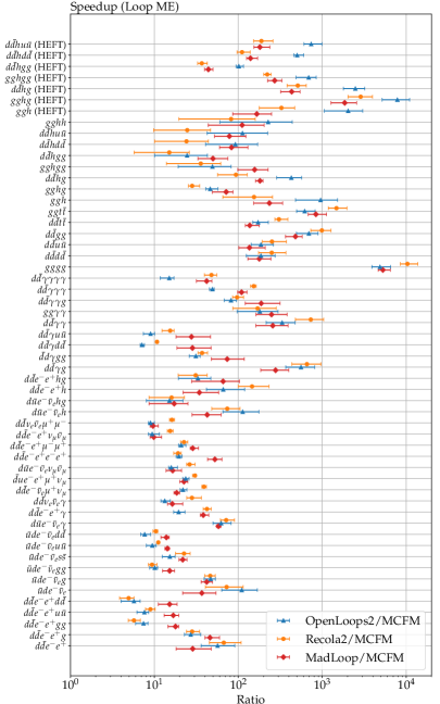
Figure 1: CPU time ratio of O

PEN

L

OOPS

, R

ECOLA

, and M

AD

L

OOP

5 to M

CFM

at the level of loop matrix elements.

Figure 2: CPU time ratio of O

PEN

L

OOPS

2, R

ECOLA

2 ${}^{\text{\scriptsize{5}}}$, and M

AD

L

OOP

5 to M

CFM

at the level of Born-like contributions to the NLO cross section (BVI).

We perform a second set of tests, using the S HERPA event generator Gleisberg et al. (2009); Bothmann et al. (2019), its existing OLP interfaces to O PEN L OOPS 2 and R ECOLA 2   Biedermann et al. (2017), and a dedicated interface to M AD L OOP 5 . With these interfaces we test the speedup in the calculation of the Born-like contributions to a typical NLO computation for the LHC at $\sqrt{s}=14$ TeV, involving the loop matrix elements in Tabs. 1 and 2. The scale choices and phase-space cuts used in these calculations are listed in App. A. Figure 2 shows the respective timing ratios. It is apparent that the large gains observed in Fig. 1 persist in this setup, because the Born-like contributions to the NLO cross section consist of the Born, integrated subtraction terms, collinear mass factorization counterterms and virtual corrections (BVI), and the timing is dominated by the loop matrix elements if at least one parton is present in the final state at Born level. The usage of M CFM speeds up the calculation by a large factor compared to the automated OLPs, with the exception of very simple processes, such as $pp\to\ell\mathrm{bar}{\ell}$, $pp\to h$, etc., where the overhead from process management and integration in Sherpa dominates. To assess this overhead we also compute the timing ratios after subtracting the time that the Sherpa computation would take without a loop matrix element. The corresponding results are shown in a lighter shade and confirm that the Sherpa overhead is significant at low multiplicity and becomes irrelevant at higher multiplicity.

In the final set of tests we investigate a typical use case in the context of parton-level event generation for LHC experiments. We use the S HERPA event generator in a multi-jet merging setup for $pp\to W$+jets and $pp\to Z$+jets Höche et al. (2013) at $\sqrt{s}=8$ TeV, with a jet separation cut of $Q_{\rm cut}=20$ GeV, and a maximum number of five final state jets at the matrix-element level. Up to two-jet final states are computed at NLO accuracy. In this use case, the gains observed in Figs. 1 and 2 will be greatly diminished, because the timing is dominated by the event generation efficiency for the highest multiplicity tree-level matrix elements Höche et al. (2019) and influenced by particle-level event generation as well as the clustering algorithm needed for multi-jet merging. We make use of the efficiency improvements described in Ref. Danziger (2020), in particular neglecting color and spin correlations in the S-MC@NLO matching procedure Höche et al. (2012). We do not include underlying event simulation or hadronization. The results in Tab. 3 still show a fairly substantial speedup when using M CFM . We point out that a higher gain could be achieved by also making use of M CFM ’s implementation of analytic matrix elements for real-emission corrections and Catani-Seymour dipole terms.

Table 3: CPU time ratios in an NLO multi-jet merged setup using S

HERPA

.

Merged Process	S HERPA $+$	S HERPA $+$
$n\leq 2~{}@~{}\mathrm{NLO}$	$\nicefrac{{O\scalebox{0.8}{PEN}L\scalebox{0.8}{OOPS}2}}{{M\scalebox{0.8}{CFM}}}$	$\nicefrac{{M\scalebox{0.8}{AD}L\scalebox{0.8}{OOP}5}}{{M\scalebox{0.8}{CFM}}}$
$n\leq 5~{}@~{}\mathrm{LO}$
$pp\to Z+nj$	$1.83^{+0.20}_{-0.12}$	$3.01^{+0.26}_{-0.18}$
$pp\to W^{+}+nj$	$1.34^{+0.06}_{-0.07}$	$1.36^{+0.03}_{-0.03}$
$pp\to W^{-}+nj$	$1.38^{+0.06}_{-0.04}$	$1.38^{+0.07}_{-0.11}$

We close this section with a direct comparison of the CPU time needed for the calculation of Drell-Yan processes with one and two jets using S HERPA and M CFM , up to a target precision on the integration of $0.1$% (one jet) or $0.3$% (two jets). The center-of-mass energy is $\sqrt{s}=14$ TeV, and the scale choices and cuts are listed in App. A. The results are shown in Tab. 4. As might be expected when comparing a dedicated parton-level code with a general-purpose particle-level generator, M CFM is substantially faster than S HERPA for the evaluation of all contributions to the NLO calculation. These results indicate a few avenues for further improvements of general-purpose event generators. With the efficient evaluation of virtual contributions in hand, attention should now turn to the calculation of real-radiation configurations – that represent the bottleneck for both S HERPA and M CFM . In the simplest cases with up to 5 partons, the real radiation and dipole counterterms could be evaluated using analytic rather than numerical matrix elements, by a suitable extension of the interface we have presented here. In addition, the form of the phase-space generation may be improved for Born-like phase-space integrals. Table 4 lists the number of phase-space points before cuts that are required to achieve the target accuracy. We find that M CFM uses fewer than half of the points needed by S HERPA in the Born-like phase-space integrals, while S HERPA uses fewer points than M CFM in the real-emission type integrals but at a much higher computational cost. This confirms that S HERPA ’s event generation is indeed impaired by the slow evaluation of real-emission type matrix elements, and by the factorial scaling of the diagram-based phase-space integration technique Byckling and Kajantie (1969a, b) used in its calculations.

Table 4: Comparison of integration times using S

HERPA

and M

CFM

.

Process		S HERPA	M CFM
MC accuracy		time / #pts	time / #pts
$pp\to Zj$	Born-like	$76.8~{}\mathrm{m}$ / 11.3M	$13.6~{}\mathrm{m}$ /4.5M
0.1%	real-like	$38~{}\mathrm{h}$ / 33.1M	$51.5~{}\mathrm{m}$ / 22.5M
$pp\to Zjj$	Born-like	$96.0~{}\mathrm{h}$ / 22.4M	$19.6~{}\mathrm{h}$ / 4.5M
0.3%	real-like	$830.4~{}\mathrm{h}$ / 58.7M	$62.9~{}\mathrm{h}$ / 83.8M
$pp\to W^{+}j$	Born-like	$40.5~{}\mathrm{m}$ / 12.8M	$7.37~{}\mathrm{m}$ / 4.5M
0.1%	real-like	$16.9~{}\mathrm{h}$ / 38.3M	$59.4~{}\mathrm{m}$ / 36.0M
$pp\to W^{+}jj$	Born-like	$14.1~{}\mathrm{h}$ / 20.3M	$9.32~{}\mathrm{h}$ / 7.2M
0.3%	real-like	$222.1~{}\mathrm{h}$ / 38.9M	$54.4~{}\mathrm{h}$ / 119.8M
$pp\to W^{-}j$	Born-like	$34.1~{}\mathrm{m}$ / 11.0M	$7.46~{}\mathrm{m}$ / 4.5M
0.1%	real-like	$15.9~{}\mathrm{h}$ / 40.5M	$47.2~{}\mathrm{m}$ / 28.1M
$pp\to W^{-}jj$	Born-like	$12.8~{}\mathrm{h}$ / 20.0M	$7.34~{}\mathrm{h}$ / 5.6M
0.3%	real-like	$281.1~{}\mathrm{h}$ / 52.0M	$38.8~{}\mathrm{h}$ / 83.8M

IV Numerical Stability

As alluded to above, the numerical stability of one-loop amplitudes is of vital importance for both NLO and NNLO calculations, where the latter case necessitates a stable evaluation in single-unresolved phase-space regions. Here we wish to limit the discussion to this case and estimate the accuracy that can be expected from the one-loop amplitudes with an additional parton with respect to the Born multiplicity, i.e., those processses that correspond to the real-virtual contribution in an NNLO calculation. To this end, we generate trajectories into the singular limits according to dipole kinematics, rescaling the Catani-Seymour variables of an initially hard configuration as

$$y_{ijk}\to\begin{cases}\lambda\frac{s}{Q^{2}}&\mathrm{final-final}\\ \frac{1}{1+\frac{Q^{2}(1-y_{ijk})}{\lambda s}}&\mathrm{final-initial}\\ -z_{i}\frac{\lambda}{1-z_{i}\lambda}&\mathrm{initial-final}\end{cases}\,,\quad z_{i}\to z_{i}$$ (1)

in the collinear limit, and

$$y_{ijk} \to\begin{cases}\frac{C(1-z_{i})}{z_{i}}&\mathrm{final-final}\\ \mathrm{sign}(y_{ijk})C\frac{1-z_{i}}{z_{i}}&\mathrm{initial-initial}\end{cases}\,,$$

$$\quad z_{i} \to\begin{cases}1-2\frac{\lambda}{1+C}&\mathrm{final-final}\\ \frac{1}{1+2\frac{\lambda^{2}-\lambda\sqrt{1+\lambda^{2}}}{1+C}}&\mathrm{initial-initial}\end{cases}\,,$$ (2)

$$C =\frac{y_{ijk}z_{i}}{1-z_{i}}$$

in the soft limit. To assess the stability of the interface, we calculate the number of stable digits as

$$N_{\text{sd}}=-\log_{10}\left(\frac{|V-V^{\prime}|}{V}\right)\,,$$ (3)

where $V$ and $V^{\prime}$ denote the finite parts of the one-loop amplitude evaluated on two phase-space points that are rotated with respect to each other.

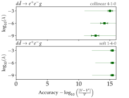
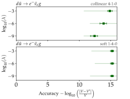
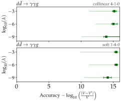
Figure 3: Test of the numerical accuracy of standard-model three-parton one-loop amplitudes in the soft and collinear limits.

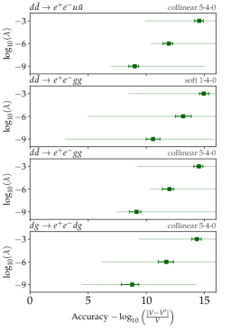
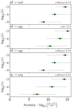
Figure 4: Test of the numerical accuracy of standard-model four-parton one-loop amplitudes in the soft and collinear limits.

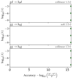
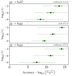
Figure 5: Test of the numerical accuracy of HEFT three- and four-parton one-loop amplitudes in the soft and collinear limits. Note that the accuracy is set to 16 digits in the $h_{0}+j$ case, where the two results agree perfectly.

We consider crossings of the processes listed in Tables 1 and 2 such that only final-state singularities are considered. We have validated that the numerical accuracy is generally worse when approaching final-state singularities, so that we deem this simplification sufficient. For each singular limit, we generate $10^{4}$ hard phase-space points with $\sqrt{s}=1~{}\mathrm{T}e\mathrm{V}$ using S HERPA and, depending on the singular limit of interest, rescale the momenta according to Eq. 1 or Eq. 2 with $\lambda\in\{10^{-3},10^{-6},10^{-9}\}$. The results are collected in Fig. 3 to Fig. 5, where each point corresponds to the average numerical accuracy according to Eq. 3 and the solid error bars indicate the $25\%$ quantiles of the median. The lighter-shaded error bands span from the worst to the best result in each run. In cases where the two results agree perfectly within machine precision, we set the number of stable digits to 16.

For all processes of interest, the numerical evaluation is sufficiently stable even in the deep infrared regions. Although not shown in the figures, we have checked that the stability of our interface is comparable to that of the other OLPs shown in Fig. 1 and Fig. 2 using appropriate settings.

V Conclusions

We have presented a novel C++ interface to the well-known M CFM parton-level Monte Carlo generator, giving access to its extensive library of analytical one-loop amplitudes. The interface is generic and not tied to any specific Monte Carlo event generation tool. As a proof of its generality, we have implemented the interface in both, the S HERPA and P YTHIA event generators. The S HERPA interface will become public with version 3.0.0, and the P YTHIA interface is foreseen to become public in a future release of the 8.3 series. It should be straightforward to adapt our code to the needs of other event generators.

We expect the interface to be valuable in two respects. First, for many of the processes considered here the speedup over other OLPs is substantial; accessing these matrix elements via this interface rather than an automated tool will therefore provide an immediate acceleration of event generation for many processes of high phenomenological interest. Second, the speed comparisons presented here highlight processes that are particularly computationally intensive for automated tools. Further improvements to the efficiency of these codes may be possible, with potential gains across a wider range of processes.

The structure of the interface allows for simple extensions. Further one-loop matrix elements in M CFM , implemented either currently or in the future, may become accessible in a straightforward manner. In the same spirit, the interface could also be extended to provide tree-level or two-loop matrix elements included in M CFM as the need arises. Further extensions to the interface, for instance to provide finer control over the one-loop matrix elements via the selection of helicities or color configurations, would also be possible.

Given that we have interfaced three popular automated OLPs within the generator-agnostic structure of the new M CFM interface, it is natural to envision the future development of a hybrid program that makes use of the fastest matrix element library for each process. Thinking further ahead, it may be worthwhile to reconsider a streamlined event generation framework, combining different (dedicated) parton-level and particle-level tools. This idea has been pursued with ThePEG Lönnblad (2006), but so far rarely deployed. Apart from obvious efficiency improvements through the use of dedicated tools for different applications, such a framework enables previously unavailable methods for systematics studies. In view of both the faster integration in M CFM over S HERPA and the magnitude of uncertainties pertaining to theoretical modeling of collider observables, this is becoming an increasingly important avenue for future work.

We want to close by highlighting that only a relatively small number of analytical amplitudes has to be known in order to cover a wide range of physical processes. When judiciously assembled, many parts of the calculations can be recycled in a process-independent way, with only charge and coupling factors being process-specific. Compared to other efforts to increase the efficiency of event generators, swapping automated for analytical matrix elements is straightforward and simple. Analytical matrix element libraries provide a so-far little explored path towards higher-efficiency event generation for the (high-luminosity) LHC and future colliders.

Appendix A Parameters and cuts for timing comparisons

In order to perform the timing comparisons shown in Fig. 2 and Table 4. we employ the following scale choices and phase-space cuts:

• $\Delta R_{\ell,\gamma}>0.4$

• $\Delta R_{\gamma,\gamma}>0.4$

• $p_{\mathrm{T},\gamma}>30~{}\mathrm{GeV}$

• $p_{\mathrm{T},j}>30~{}\mathrm{GeV}$

• $66~{}\mathrm{GeV}<m_{\ell\mathrm{bar}{\ell}}<116~{}\mathrm{GeV}$

We reconstruct jets using the anti-$k_{\mathrm{T}}$ algorithm Cacciari et al. (2008) in the implementation of FastJet Cacciari et al. (2012) with an $R$ parameter of 0.4. For the di-jet process we require $p_{\mathrm{T},j}>$80 GeV. Photons are isolated from QCD activity based on Ref. Frixione (1998) with $\delta_{0}$=0.4, $n$=2 and $\epsilon_{\gamma}$=2.5%

Appendix B Structure of the interface

The M CFM C++ interface is constructed as a C++ class

⬇

CXX_Interface mcfm;

included in the header:

⬇

#include "MCFM/CXX_Interface.h"

It must be initialized on a std::map of std::strings, containing all (standard-model) parameters:

⬇

bool CXX_Interface::Initialize(

std::map<std::string,std::string>& parameters);

Prior to use, each process has to be initialized in the interface:

⬇

int CXX_Interface::InitializeProcess(const Process_Info &pi);

which takes a Process_Info object as input, which in turn contains the defining parameters of a given process, i.e., the PDG IDs, number of incoming particles, and QCD and EW coupling orders:

⬇

Process_Info(const std::vector<int> &ids, const int nin,

const int oqcd, const int oew);

Phase space points are defined using the FourVec struct, which represents four-vectors in the ordering $(E,p_{x},p_{y},p_{z})$.

⬇

FourVec(double e, double px, double py, double pz);

Given a list of four-vectors in this format, one-loop matrix elements can be calculated either using the process ID returned by the InitializeProcess method

⬇

void CXX_Interface::Calc(int procID,

const std::vector<FourVec> &p, int oqcd);

or using a Process_Info struct:

⬇

void CXX_Interface::Calc(const Process_Info &pi,

const std::vector<FourVec> &p,int oqcd);

In the same way, the result of this calculation can be accessed either via the process ID

⬇

const std::vector<double> &CXX_Interface::GetResult(int procID);

or using the Process_Info struct:

⬇

const std::vector<double> &CXX_Interface::GetResult(const Process_Info &pi)

The result is returned as a list of Laurent series coefficients in the format $(\mathcal{O}\left(\varepsilon^{0}\right),\mathcal{O}\left(\varepsilon^{-1}\right),\mathcal{O}\left(\varepsilon^{-2}\right),\mathrm{Born})$. However, by default only the $\mathcal{O}\left(\varepsilon^{0}\right)$ coefficient, i.e., the finite part, is returned. The calculation of the pole terms and the Born can be enabled by setting the following switch to 1:

⬇

void CXX_Interface::SetPoleCheck(int check);

An example code showing the basic usage of the interface as well as a function filling the complete list of parameters with default values is publicly available.

References

- Berger et al. (2008) C. F. Berger, Z. Bern, L. J. Dixon, F. Febres Cordero, D. Forde, H. Ita, D. A. Kosower, and D. Maître, Phys. Rev. D 78, 036003 (2008), arXiv:0803.4180 [hep-ph] .
- Berger et al. (2009) C. F. Berger, Z. Bern, L. J. Dixon, F. Febres Cordero, D. Forde, T. Gleisberg, H. Ita, D. A. Kosower, and D. Maître, Phys. Rev. D 80, 074036 (2009), arXiv:0907.1984 [hep-ph] .
- Berger et al. (2010) C. F. Berger, Z. Bern, L. J. Dixon, F. Febres Cordero, D. Forde, T. Gleisberg, H. Ita, D. A. Kosower, and D. Maître, Phys. Rev. D 82, 074002 (2010), arXiv:1004.1659 [hep-ph] .
- Berger et al. (2011) C. F. Berger, Z. Bern, L. J. Dixon, F. Febres Cordero, D. Forde, T. Gleisberg, H. Ita, D. A. Kosower, and D. Maître, Phys. Rev. Lett. 106, 092001 (2011), arXiv:1009.2338 [hep-ph] .
- Ita et al. (2012) H. Ita, Z. Bern, L. J. Dixon, F. Febres Cordero, D. A. Kosower, and D. Maître, Phys. Rev. D 85, 031501 (2012), arXiv:1108.2229 [hep-ph] .
- Bern et al. (2013) Z. Bern, L. J. Dixon, F. Febres Cordero, S. Höche, H. Ita, D. A. Kosower, D. Maître, and K. J. Ozeren, Phys. Rev. D 88, 014025 (2013), arXiv:1304.1253 [hep-ph] .
- Hirschi et al. (2011) V. Hirschi, R. Frederix, S. Frixione, M. V. Garzelli, F. Maltoni, and R. Pittau, JHEP 05, 044 (2011), arXiv:1103.0621 [hep-ph] .
- Alwall et al. (2014) J. Alwall, R. Frederix, S. Frixione, V. Hirschi, F. Maltoni, O. Mattelaer, H. S. Shao, T. Stelzer, P. Torrielli, and M. Zaro, JHEP 07, 079 (2014), arXiv:1405.0301 [hep-ph] .
- Cascioli et al. (2012) F. Cascioli, P. Maierhöfer, and S. Pozzorini, Phys. Rev. Lett. 108, 111601 (2012), arXiv:1111.5206 [hep-ph] .
- Buccioni et al. (2018) F. Buccioni, S. Pozzorini, and M. Zoller, Eur. Phys. J. C 78, 70 (2018), arXiv:1710.11452 [hep-ph] .
- Buccioni et al. (2019) F. Buccioni, J.-N. Lang, J. M. Lindert, P. Maierhöfer, S. Pozzorini, H. Zhang, and M. F. Zoller, Eur. Phys. J. C 79, 866 (2019), arXiv:1907.13071 [hep-ph] .
- Badger et al. (2011) S. Badger, B. Biedermann, and P. Uwer, Comput. Phys. Commun. 182, 1674 (2011), arXiv:1011.2900 [hep-ph] .
- Badger et al. (2013) S. Badger, B. Biedermann, P. Uwer, and V. Yundin, Comput. Phys. Commun. 184, 1981 (2013), arXiv:1209.0100 [hep-ph] .
- Cullen et al. (2012) G. Cullen, N. Greiner, G. Heinrich, G. Luisoni, P. Mastrolia, G. Ossola, T. Reiter, and F. Tramontano, Eur. Phys. J. C 72, 1889 (2012), arXiv:1111.2034 [hep-ph] .
- Cullen et al. (2014) G. Cullen et al., Eur. Phys. J. C 74, 3001 (2014), arXiv:1404.7096 [hep-ph] .
- Actis et al. (2013) S. Actis, A. Denner, L. Hofer, A. Scharf, and S. Uccirati, JHEP 04, 037 (2013), arXiv:1211.6316 [hep-ph] .
- Actis et al. (2017) S. Actis, A. Denner, L. Hofer, J.-N. Lang, A. Scharf, and S. Uccirati, Comput. Phys. Commun. 214, 140 (2017), arXiv:1605.01090 [hep-ph] .
- Denner et al. (2017) A. Denner, J.-N. Lang, and S. Uccirati, JHEP 07, 087 (2017), arXiv:1705.06053 [hep-ph] .
- Denner et al. (2018) A. Denner, J.-N. Lang, and S. Uccirati, Comput. Phys. Commun. 224, 346 (2018), arXiv:1711.07388 [hep-ph] .
- Degrande (2015) C. Degrande, Comput. Phys. Commun. 197, 239 (2015), arXiv:1406.3030 [hep-ph] .
- Degrande et al. (2020) C. Degrande, G. Durieux, F. Maltoni, K. Mimasu, E. Vryonidou, and C. Zhang, (2020), arXiv:2008.11743 [hep-ph] .
- Albrecht et al. (2019) J. Albrecht et al. (HEP Software Foundation), Comput. Softw. Big Sci. 3, 7 (2019), arXiv:1712.06982 [physics.comp-ph] .
- Alioli et al. (2019) S. Alioli et al., (2019), arXiv:1902.01674 [hep-ph] .
- Amoroso et al. (2021) S. Amoroso et al. (HSF Physics Event Generator WG), Comput. Softw. Big Sci. 5, 12 (2021), arXiv:2004.13687 [hep-ph] .
- Aarrestad et al. (2020) T. Aarrestad et al. (HEP Software Foundation), in 2022 Snowmass Summer Study, edited by P. Canal et al. (2020) arXiv:2008.13636 [physics.comp-ph] .
- Boughezal et al. (2017) R. Boughezal, J. M. Campbell, R. K. Ellis, C. Focke, W. Giele, X. Liu, F. Petriello, and C. Williams, Eur. Phys. J. C 77, 7 (2017), arXiv:1605.08011 [hep-ph] .
- Campbell and Neumann (2019) J. Campbell and T. Neumann, JHEP 12, 034 (2019), arXiv:1909.09117 [hep-ph] .
- Campbell and Ellis (1999) J. M. Campbell and R. K. Ellis, Phys. Rev. D 60, 113006 (1999), arXiv:hep-ph/9905386 .
- Campbell et al. (2011) J. M. Campbell, R. K. Ellis, and C. Williams, JHEP 07, 018 (2011), arXiv:1105.0020 [hep-ph] .
- Campbell et al. (2015) J. M. Campbell, R. K. Ellis, and W. T. Giele, Eur. Phys. J. C 75, 246 (2015), arXiv:1503.06182 [physics.comp-ph] .
- Binoth et al. (2010) T. Binoth et al., Comput. Phys. Commun. 181, 1612 (2010), arXiv:1001.1307 [hep-ph] .
- Alioli et al. (2014) S. Alioli et al., Comput. Phys. Commun. 185, 560 (2014), arXiv:1308.3462 [hep-ph] .
- Bothmann et al. (2019) E. Bothmann et al. (Sherpa), SciPost Phys. 7, 034 (2019), arXiv:1905.09127 [hep-ph] .
- Sjöstrand et al. (2015) T. Sjöstrand, S. Ask, J. R. Christiansen, R. Corke, N. Desai, P. Ilten, S. Mrenna, S. Prestel, C. O. Rasmussen, and P. Z. Skands, Comput. Phys. Commun. 191, 159 (2015), arXiv:1410.3012 [hep-ph] .
- Hartgring et al. (2013) L. Hartgring, E. Laenen, and P. Skands, JHEP 10, 127 (2013), arXiv:1303.4974 [hep-ph] .
- Baberuxki et al. (2020) N. Baberuxki, C. T. Preuss, D. Reichelt, and S. Schumann, JHEP 04, 112 (2020), arXiv:1912.09396 [hep-ph] .
- Brooks et al. (2020) H. Brooks, C. T. Preuss, and P. Skands, JHEP 07, 032 (2020), arXiv:2003.00702 [hep-ph] .
- Campbell et al. (2017) J. M. Campbell, R. K. Ellis, and C. Williams, Phys. Rev. Lett. 118, 222001 (2017), [Erratum: Phys.Rev.Lett. 124, 259901 (2020)], arXiv:1612.04333 [hep-ph] .
- (39) J. Campbell, K. Ellis, W. Giele, T. Neumann, and C. Williams, https://mcfm.fnal.gov/.
- Denner et al. (1999) A. Denner, S. Dittmaier, M. Roth, and D. Wackeroth, Nucl. Phys. B 560, 33 (1999), arXiv:hep-ph/9904472 .
- Denner et al. (2005) A. Denner, S. Dittmaier, M. Roth, and L. H. Wieders, Nucl. Phys. B 724, 247 (2005), [Erratum: Nucl.Phys.B 854, 504–507 (2012)], arXiv:hep-ph/0505042 .
- Bern et al. (1998) Z. Bern, L. J. Dixon, and D. A. Kosower, Nucl. Phys. B 513, 3 (1998), arXiv:hep-ph/9708239 .
- Campbell and Ellis (2017) J. M. Campbell and R. K. Ellis, JHEP 01, 020 (2017), arXiv:1610.02189 [hep-ph] .
- Ellis et al. (1988) R. K. Ellis, I. Hinchliffe, M. Soldate, and J. J. van der Bij, Nucl. Phys. B 297, 221 (1988).
- Ellis and Seth (2018) R. K. Ellis and S. Seth, JHEP 11, 006 (2018), arXiv:1808.09292 [hep-ph] .
- Budge et al. (2020) L. Budge, J. M. Campbell, G. De Laurentis, R. K. Ellis, and S. Seth, JHEP 05, 079 (2020), arXiv:2002.04018 [hep-ph] .
- Glover and van der Bij (1988) E. Glover and J. J. van der Bij, Nucl. Phys. B 309, 282 (1988).
- Campbell et al. (2016a) J. M. Campbell, R. K. Ellis, and C. Williams, JHEP 06, 179 (2016a), arXiv:1601.00658 [hep-ph] .
- Ellis et al. (1981) R. K. Ellis, D. A. Ross, and A. E. Terrano, Nucl. Phys. B 178, 421 (1981).
- Aurenche et al. (1987) P. Aurenche, R. Baier, A. Douiri, M. Fontannaz, and D. Schiff, Nucl. Phys. B 286, 553 (1987).
- Campbell et al. (2016b) J. M. Campbell, R. K. Ellis, Y. Li, and C. Williams, JHEP 07, 148 (2016b), arXiv:1603.02663 [hep-ph] .
- Campbell and Williams (2014) J. M. Campbell and C. Williams, Phys. Rev. D 89, 113001 (2014), arXiv:1403.2641 [hep-ph] .
- Dennen and Williams (2015) T. Dennen and C. Williams, Phys. Rev. D 91, 054012 (2015), arXiv:1411.3237 [hep-ph] .
- Dixon et al. (1998) L. J. Dixon, Z. Kunszt, and A. Signer, Nucl. Phys. B 531, 3 (1998), arXiv:hep-ph/9803250 .
- Nason et al. (1989) P. Nason, S. Dawson, and R. K. Ellis, Nucl. Phys. B 327, 49 (1989), [Erratum: Nucl.Phys.B 335, 260–260 (1990)].
- Ellis and Sexton (1986) R. K. Ellis and J. C. Sexton, Nucl. Phys. B 269, 445 (1986).
- Schmidt (1997) C. R. Schmidt, Phys. Lett. B 413, 391 (1997), arXiv:hep-ph/9707448 .
- Dixon et al. (2004) L. J. Dixon, E. Glover, and V. V. Khoze, JHEP 12, 015 (2004), arXiv:hep-th/0411092 .
- Ellis et al. (2005) R. K. Ellis, W. T. Giele, and G. Zanderighi, Phys. Rev. D 72, 054018 (2005), [Erratum: Phys.Rev.D 74, 079902 (2006)], arXiv:hep-ph/0506196 .
- Badger and Glover (2006) S. D. Badger and E. Glover, Nucl. Phys. B Proc. Suppl. 160, 71 (2006), arXiv:hep-ph/0607139 .
- Badger et al. (2007) S. D. Badger, E. Glover, and K. Risager, JHEP 07, 066 (2007), arXiv:0704.3914 [hep-ph] .
- Glover et al. (2008) E. Glover, P. Mastrolia, and C. Williams, JHEP 08, 017 (2008), arXiv:0804.4149 [hep-ph] .
- Badger et al. (2010) S. Badger, E. Glover, P. Mastrolia, and C. Williams, JHEP 01, 036 (2010), arXiv:0909.4475 [hep-ph] .
- Dixon and Sofianatos (2009) L. J. Dixon and Y. Sofianatos, JHEP 08, 058 (2009), arXiv:0906.0008 [hep-ph] .
- Badger et al. (2009) S. Badger, J. M. Campbell, R. K. Ellis, and C. Williams, JHEP 12, 035 (2009), arXiv:0910.4481 [hep-ph] .
- Kleiss et al. (1986) R. Kleiss, W. J. Stirling, and S. D. Ellis, Comput. Phys. Commun. 40, 359 (1986).
- Gleisberg et al. (2009) T. Gleisberg, S. Höche, F. Krauss, M. Schönherr, S. Schumann, F. Siegert, and J. Winter, JHEP 02, 007 (2009), arXiv:0811.4622 [hep-ph] .
- Biedermann et al. (2017) B. Biedermann, S. Bräuer, A. Denner, M. Pellen, S. Schumann, and J. M. Thompson, Eur. Phys. J. C 77, 492 (2017), arXiv:1704.05783 [hep-ph] .
- Höche et al. (2013) S. Höche, F. Krauss, M. Schönherr, and F. Siegert, JHEP 04, 027 (2013), arXiv:1207.5030 [hep-ph] .
- Höche et al. (2019) S. Höche, S. Prestel, and H. Schulz, Phys. Rev. D 100, 014024 (2019), arXiv:1905.05120 [hep-ph] .
- Bothmann et al. (2016) E. Bothmann, M. Schönherr, and S. Schumann, Eur. Phys. J. C 76, 590 (2016), arXiv:1606.08753 [hep-ph] .
- Bothmann et al. (2021) E. Bothmann, S. Höche, and M. Schönherr, (2021).
- Danziger (2020) K. Danziger, (2020), https://cds.cern.ch/record/2715727.
- Höche et al. (2012) S. Höche, F. Krauss, M. Schönherr, and F. Siegert, JHEP 09, 049 (2012), arXiv:1111.1220 [hep-ph] .
- Byckling and Kajantie (1969a) E. Byckling and K. Kajantie, Nucl. Phys. B9, 568 (1969a).
- Byckling and Kajantie (1969b) E. Byckling and K. Kajantie, Phys.Rev. 187, 2008 (1969b).
- Gleisberg and Höche (2008) T. Gleisberg and S. Höche, JHEP 12, 039 (2008), arXiv:0808.3674 [hep-ph] .
- Lönnblad (2006) L. Lönnblad, Nucl. Instrum. Meth. A 559, 246 (2006).
- Cacciari et al. (2008) M. Cacciari, G. P. Salam, and G. Soyez, JHEP 04, 063 (2008), arXiv:0802.1189 [hep-ph] .
- Cacciari et al. (2012) M. Cacciari, G. P. Salam, and G. Soyez, Eur. Phys. J. C 72, 1896 (2012), arXiv:1111.6097 [hep-ph] .
- Frixione (1998) S. Frixione, Phys. Lett. B 429, 369 (1998), arXiv:hep-ph/9801442 .