Accelerating LHC event generation
with simplified pilot runs and fast PDFs

Abstract

Poor computing efficiency of precision event generators for LHC physics has become a bottleneck for Monte-Carlo event simulation campaigns. We provide solutions to this problem by focusing on two major components of general-purpose event generators: The PDF evaluator and the matrix-element generator. For a typical production setup in the ATLAS experiment, we show that the two can consume about 80% of the total runtime. Using NLO simulations of $pp\to\ell^{+}\ell^{-}+\text{jets}$ and $pp\to t\bar{t}+\text{jets}$ as an example, we demonstrate that the computing footprint of L HAPDF and S HERPA can be reduced by factors of order 10, while maintaining the formal accuracy of the event sample. The improved codes are made publicly available.

1 Introduction

Particle colliders have long dominated efforts to experimentally probe fundamental interactions at the energy frontier. They enable access to the highest energy scales in human-made experiments, at high collision rates and in controlled conditions, allowing a systematic investigation of the most basic laws of physics. Event-generator programs have come to play a crucial role in such experiments, starting with the use of early event generators such as JETSET [1] and HERWIG [2] in the discovery of the gluon at the PETRA facility in 1979.

Today, with the Large Hadron Collider (LHC) having operated successfully for over a decade at nearly 1000 times the energy of PETRA, event generators are an ever more important component of the software stack needed to extract fundamental physics parameters from experimental data [3, 4]. Most experimental measurements rely on their precise modelling of complete particle-level events on which a detailed detector simulation can be applied. The experimental demands on these tools continue to grow: the precision targets of the high-luminosity LHC (HL-LHC)  [5] will require both high theoretical precision and large statistical accuracy, presenting major challenges for the currently available generator codes. With much of the development during the past decades having focused on improvements in theoretical precision—in terms of the formal accuracy of the elements of the calculation—their computing performance has become a major concern [6, 7, 8, 9].

Event generators are constructed in a modular fashion, which is inspired by the description of the collision events in terms of different QCD dynamics at different energy scales. At the highest scales, computations can be carried out using amplitudes calculated in QCD perturbation theory. These calculations have been largely automated in matrix-element generators, both at leading [10, 11, 12, 13, 14], and at next-to-leading [15, 16, 17, 18, 19, 20] orders in the strong coupling constant, $\alpha_{s}$. Matrix-element generators perform the dual tasks of computing scattering matrix elements fully differentially in the particle momenta, as well as integrating these differential functions over the multi-particle phase space using Monte Carlo (MC) methods.

In principle, such calculations can be carried out for an arbitrary number of final-state particles; in practice, the tractable multiplicities are very limited. The presence of quantum interference effects in the matrix elements induces an exponential scaling of computation complexity with the number of final-state particles. This problem is exacerbated further by the rise of automatically calculated next-to-leading order (NLO) matrix elements in the QCD and electroweak (EW) couplings, which not only have a higher intrinsic cost from more complex expressions, but are also more difficult to efficiently sample in phase-space, and introduce potentially negative event weights which reduce the statistical power of the resulting event samples. While theoretical work progresses on these problems, e.g. by the introduction of rejection sampling using neural network event-weight estimates [21], modified parton-shower matching schemes [22, 23] and resampling techniques [24, 25], the net effect remains that precision MC event generation comes at a computational cost far higher than in previous simulation campaigns. Indeed, it already accounts for a significant fraction of the total LHC computing budget [26, 9], and there is a real risk that the physics achievable with data from the high-luminosity runs of the LHC will be limited by the size of MC event samples that can be generated within fixed computing budgets. It is therefore crucial that dedicated attention is paid to issues of computational efficiency.

In this article, we focus on computational strategies to improve the performance of particle-level MC event generator programs, as used to produce large high-precision simulated event samples at the LHC. While the strategies and observations are of a general nature, we focus our attention on concrete implementations in the S HERPA event generator [27] and the L HAPDF library for parton distribution function (PDF) evaluation [28]. Collectively, this effort is aimed at solving the current computational bottlenecks in LHC high-precision event generation. Using generator settings for standard-candle processes from the ATLAS experiment [29] as a baseline, we discuss timing improvements related to PDF-uncertainty evaluation and for event generation more generally. Overall, our new algorithms provide speedups of a factor of up to 15 for the most time-consuming simulations in typical configurations, in time for the LHC Run-3 event-generation campaigns.

This manuscript is structured as follows: Section 2 discusses refinements to the L HAPDF library, including both intrinsic performance improvements and the importance of efficient call strategies. Section 3 details improvements of the S HERPA event generator. Section 4 quantifies the impact of our modifications. In Sec. 5 we discuss possible future directions for further improvements of the two software packages, and Sec. 6 provides an outlook.

2 L HAPDF performance bottlenecks and improvements

While the core machinery of event generators for high-energy collider physics is framed in terms of partonic scattering events, real-world relevance of course requires that the matrix elements be evaluated for colliding beams of hadrons. This is typically implemented through use of the collinear factorisation formula for the differential cross section about a final-state phase-space configuration $\Phi$,

$${\mathrm{d}}{\sigma({h_{1}h_{2}\to n})}=\sum_{a,b}\,\int_{0}^{1}\!{\mathrm{d}}{x_{a}}\,\int_{0}^{1}\!{\mathrm{d}}{x_{b}}~{}f_{a}^{h_{1}}(x_{a},\mu_{\mathrm{F}})\,f_{b}^{h_{2}}(x_{b},\mu_{\mathrm{F}})\,{\mathrm{d}}\hat{\sigma}_{ab\to n}(\Phi,\mu_{\mathrm{R}},\mu_{\mathrm{F}})\,,$$ (2.1)

where $x_{a,b}$ are the light-cone momentum fractions of the two incoming partons $a$ and $b$ with respect to their parent hadrons $h_{1}$ and $h_{2}$, and $\mu_{\mathrm{R,F}}$ are the renormalisation and factorisation scales, respectively. Assuming negligible transverse motion of the partons, this formula yields the hadron-level differential cross section ${\mathrm{d}}{\sigma}$ as an integral over the initial-state phase-space, summed over $a$ and $b$, weighting the differential squared matrix-element $\mathrm{d}\hat{\sigma}$ by the collinear parton densities (PDFs) $f$ for the incoming beams. These PDFs satisfy the evolution equations [30, 31, 32, 33]

$$\frac{{\rm d}\ln f_{a}^{h}(x,t)}{{\rm d}\ln t}=\sum_{b=q,g}\int_{0}^{1}\frac{{\rm d}z}{z}\,\frac{\alpha_{s}}{2\pi}P_{ab}(z)\,\frac{f_{b}^{h}(x/z,t)}{f_{a}^{h}(x,t)}\;,$$ (2.2)

with the evolution kernels, $P_{ab}(z)$, given as a power series in the strong coupling, $\alpha_{s}$.

In MC event-generation, the integrals in Eqs. (2.1) and (2.2) are replaced by MC rejection sampling, meaning that a set of PDF values $f_{a}^{h}(x,\mu_{\mathrm{F}})$ must be evaluated at every sampled phase-space point, for both beams. PDFs are hence among the most intensely called functions within an event generator code, comparable with the partonic matrix-element itself. In particular, Eq. (2.2) is iteratively solved by the backward evolution algorithm of initial-state parton showers [34], requiring two PDF calls per trial emission [35].

This intrinsic computational load is exacerbated by the additional factors that 1) the non-perturbative PDFs are not generally available as closed-form expressions, but as discretised grids of $f{}(x_{i},Q^{2}_{i})$ values obtained from fits to data via QCD scale-evolution, and 2) the PDF fits introduce many new sources of systematic uncertainty, which are typically encoded via $\mathcal{O}(10\text{--}100)$ alternative sets of PDF functions to be evaluated at the same $(x,Q^{2})$ points. In LHC MC-event production, these grids are interpolated to provide PDF values and consistent values of the running coupling, $\alpha_{s}$, through continuous $(x,Q^{2})$ space by the L HAPDF library.

The starting point for this work is L HAPDF version 6.2.3, the C++ L HAPDF 6 lineage being a redevelopment of the Fortran-based L HAPDF  $\leq 5$ series. The Fortran series relied on each PDF fit being supplied as a new subroutine by the fitting group; in principle these used a common memory space across sets, but in practice many separate such memory blocks were allocated, leading to problematically high memory demands in MC-event production. The C++ series has a more restrictive core scope, using dynamic memory allocation and a set of common interpolation routines to evaluate PDF values from grids encoded in a standard data format. Each member of a collinear PDF set is a set of functions $f_{a}^{h}(x,Q^{2})$ for each active parton flavour, $a$, and is independently evaluated within L HAPDF .

The most heavily used interpolation algorithm in L HAPDF is a 2D local-cubic polynomial [36] in $(\log x,\log Q^{2})$ space, corresponding to a composition of 1D cubic interpolations in first the $x$ and then the $Q^{2}$ direction on the grid. As each 1D interpolation requires the use of four $f_{a}(x_{i},Q_{j}^{2})$ knot values, naively 16 knots are needed as input to construct 4 values at the same $x$ value, used as the arguments for the final 1D interpolation in $\log Q^{2}$. The end result is a weighted combination of the PDF values on the 16 knots surrounding the interpolation cell of interest, with the weights as functions of the position of the evaluated point within the cell.

2.1 PDF-grid caching

The first effort to improve L HAPDF ’s evaluation efficiency was motivated by the sum over initial-state flavours in Eq. (2.1), implying that up to 11 calls (for each parton flavour, excluding the top quark) may be made near-consecutively for a fixed $(x,Q^{2})$ point within the same PDF.

If such repeated calls use the same $(x,Q^{2})$ knot positions for all flavours (which is nearly always the case), much of the weight computation described above can be cached and re-used with a potential order-of-magnitude gain. Such a caching was implemented, with a dictionary of cyclic caches stored specific to each thread and keyed on a hash-code specific to the grid spacing: this ensures that the caching works automatically across different flavours if they use the same grid geometry but does not return incorrect results should that assumption be incorrect. This implementation also has the promising side-effect that, if the set of fit-variation PDFs also use the same grid spacing as the nominal PDF, consecutive accesses of the same $(x,Q^{2})$ across possibly hundreds of PDFs would also automatically benefit from the caching.

The practicality of a cache implementation in L HAPDF (with no restructuring of the call patterns from S HERPA ) was investigated using the $e^{+}e^{-}$+jets setup described below and a 64-entry cyclic cache. This cache is too large to obtain any performance benefits but was useful to explore the caching behaviour. 57% of $x$ and 54% of $Q^{2}$ lookups were located within the 64-entry cache. Of these successful cache-hits, the cumulative probability of an $x$ hit rose linearly from 10% in the first check to 50% by the 6th check before slowing down (90% by the 51st check), as illustrated in Figure 1. For $Q^{2}$, the cumulative probability was already at 80% by the third check (90% by the 13th check).

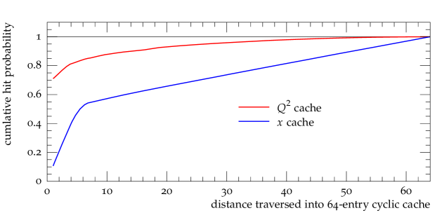
Figure 1: Cumulative probability of obtaining cache-hit as a function of search depth into a 64-entry cyclic cache for calls to $x$ and $Q^{2}$ by S HERPA when generating $e^{+}e^{-}$+jet MC events. As a proportion of all calls which resulted in a cache-hit.

Despite this promise, this caching feature as implemented in L HAPDF  6.3.0 transpired to add little if anything in practical applications with S HERPA generation of these ATLAS-like $e^{+}e^{-}$+jets MC events. With a cache depth of 4, the time spent in L HAPDF in the call-stack reduced marginally by a relative 5%, this overall reduction is small due to 29% of the time spent in L HAPDF now being under the newly added _getCacheX and _getCacheQ2 functions. This indicates that, given the S HERPA request pattern, the cost of executing the caching implementation is somewhat comparable to the cost of re-interpolating the quantity.

This experience of caching as a strategy to reduce PDF-interpolation overheads in realistic LHC use-cases highlights the importance of well-matched PDF-call strategies in the event generator. We return to this point later.

2.2 Memory structuring and return to multi-flavour caching

The C++ rewrite of L HAPDF placed emphasis on flexibility and “pluggability” of interpolators to accommodate fitting groups’ requirements, allowing the use of non-uniform grid spacings, functional discontinuities across flavour thresholds, and even different grids for each parton flavour [28], at the cost of a fragmented memory layout. However, much of this flexibility has in practice gone unused.

By disabling the possibility to have fragmented knots for differing flavours, the knots are now stored in a single structure for all flavours. Similarly, the PDF grids are stored in a combined data-structure. This will allow for very efficient caching and even memory accesses due to the contiguous memory layout.

With the observed shortcomings in the caching-strategy implemented in L HAPDF  6.3.0, as described above, in L HAPDF  6.4.0, the caching mechanism focuses on multi-flavour PDFs that are called for explicitly. In this case, large parts of the computations can be shared between the different flavour PDF (for example finding the right knot-indices and computing spacings) due to the fact that the grids have been unified. In principle, the caching of shared computations among the variations is still desirable, given that many variations share grids. However as discussed above, the call strategy of the generator then has to be structured (or, restructured) with this in mind in order to make this caching efficient.

2.3 Finite-difference precomputations

Additionally to the reworked caching strategy, L HAPDF  6.4.0 pre-computes parts of the computations and stores the results. Due to the way the local-cubic polynomial interpolation is set up, the first set of interpolations are always computed along the grid lines. Since these are always the same, in L HAPDF  6.4.0 the coefficients of the interpolation polynomial are pre-computed for the grid-aligned interpolations. This comes with the drawback of the additional memory space that is required to store the coefficients, but it also reduces the interpolation to simply the evaluation of a cubic polynomial (compared to first constructing said polynomial, and then evaluating it). The precomputations reduce the number of “proper” interpolations (in the sense that the interpolation polynomial has to be constructed) from five to one.

Because of these precomputations and the above described memory restructurings, computing the PDF becomes up to a factor of $\sim\!3$ faster for a single flavour, and with the combination of the multi-flavour caching, computing the PDFs for for all flavours becomes roughly $\sim\!10$ faster.

3 S HERPA performance bottlenecks and improvements

The computing performance of various LHC event generators was investigated in a recent study performed by the HEP software foundation [7, 8, 9]. This comparison prompted a closer inspection of the algorithms used and choices made in the Sherpa program. In this section we will briefly review the computationally most demanding parts of the simulation, provide some background information on the physics models, and offer strategies to reduce their computational complexity.

We will focus on the highly relevant processes $pp\to\ell^{+}\ell^{-}+\text{jets}$ and $pp\to t\bar{t}+\text{jets}$, described in detail in Sec. 4. They are typically simulated using NLO multi-jet merged calculations with EW virtual corrections and include scale as well as PDF variations. The baseline for our simulations is the S HERPA event generator, version 2.2.11 [37]. In the typical configuration used by the ATLAS experiment, it employs the C OMIX matrix element calculator [13] to compute leading-order cross sections with up to five final-state jets in $pp\to\ell^{+}\ell^{-}+\text{jets}$ and four jets in $pp\to t\bar{t}+\text{jets}$. Next-to-leading order precision in QCD is provided for up to two jets in $pp\to\ell^{+}\ell^{-}+\text{jets}$ and up to one jet in $pp\to t\bar{t}+\text{jets}$ with the help of the O PEN L OOPS library [18, 38] for virtual corrections and an implementation of Catani-Seymour dipole subtraction in A MEGIC  [39] and C OMIX . The matching to a Catani-Seymour based parton shower [40] is performed using the S–M C @N LO technique [41, 42], an extension of the M C @N LO matching method [43] that implements colour and spin correlations in the first parton-shower emission, in order to reproduce the exact singularity structure of the hard matrix element. In addition, EW corrections and scale-, $\alpha_{s}$- and PDF-variation multiweights are implemented using the techniques outlined in [44, 45, 46]. A typical setup includes of the order of two hundred multiweights, most of which correspond to PDF variations.

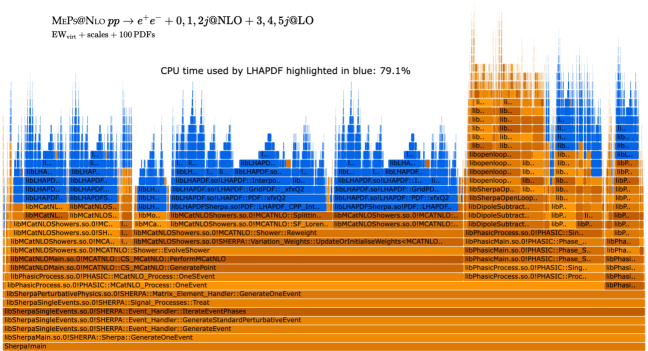
Figure 2: CPU profile of 1000 MC unweighted $pp\to e^{+}e^{-}$+jet events generated by S HERPA 2.2.11 interfaced with L HAPDF 6.2.3. The 79% of run-time spent within L HAPDF in the call-stack is highlighted in blue.

We visualize the imperfect interplay between S HERPA and L HAPDF in Fig. 2. For this test, S HERPA  2.2.11 was compiled against L HAPDF  6.2.3 and O PEN L OOPS  2.1.2 [18, 38]. The performance of generating 1000 partially unweighted MC events was then profiled with the Intel${}^{\text{\textregistered}}$ VTune™ profiler running on a single core of a $2.20\text{\,}\mathrm{G}\mathrm{H}\mathrm{z}$ Intel${}^{\text{\textregistered}}$ Xeon${}^{\text{\textregistered}}$ E5-2430. The S HERPA run card contains a representative $pp\to e^{+}e^{-}+0,1,2j$@NLO$+3,4,5j$@LO setup at $\sqrt{s}=13$ TeV, including electroweak virtual corrections as well as reweightings to different PDFs and scales; comparable to the setup used in production by the ATLAS collaboration at the time. The total processing time was around 18.5 hours.

The obtained execution profile is visualized in Figure 2 as a flame-graph [47] where the proportion of the $x$-axis reflects the proportion of wall-time spent inside a given function, and where the call-stack extends up the $y$-axis. Calls from S HERPA into the L HAPDF library are highlighted in blue. In total, $79\text{\,}\mathrm{\char 37\relax}$ of the execution time was spent in L HAPDF , with libLHAPDFSherpa.so!PDF::LHAPDF_CPP_Interface::GetXPDF representing the dominant interface call.

In the following, we discuss in detail the major efficiency improvements that have been implemented on the S HERPA side, including the solution to spending so much execution time within L HAPDF . In addition to the major changes, also some minor improvements have been developed, which account for a collective runtime savings of $510\text{\,}\mathrm{\char 37\relax}$. A notable example is the introduction of a cache for the partonic channel selection weights, reducing the necessity to resolve virtual functions in inheritance structures.

3.1 Leading-colour matched emission

A simple strategy to improve the performance of the S–M C @N LO matching was recently discussed in [23]. Within the S–M C @N LO technique, one requires the parton shower to reconstruct the exact soft radiation pattern obtained in the NLO result. In processes with more than two coloured particles, this leads to non-trivial radiator functions, which are given in terms of eikonals obtained from quasi-classical currents [48]. Due to the involved colour structure of the related colour insertion operators, the radiation pattern can typically not be captured by standard parton shower algorithms. The S–M C @N LO technique relies on weighted parton showers [49] to solve this problem. As both the sign and the magnitude of the colour correlators can differ from the Casimir operator used in leading colour parton showers, the weights can become negative and are in general prone to large fluctuations that need to be included in the overall event weight, thus lowering the unweighting efficiency and reducing the statistical power of the event sample.

This problem can be circumvented by assuming that experimentally relevant observables will likely not be capable of resolving the details of soft radiation, and that colour factors in the collinear (and soft-collinear) limit are given in terms of Casimir operators. This idea is also used in the original M C @N LO method [43] to enable the matching to parton showers which do not have the correct soft radiation pattern. Within S HERPA , the S–M C @N LO matching is simplified to an M C @N LO matching, dubbed $\langle\text{LC}\rangle$–M C @N LO here, using the setting NLO_CSS_PSMODE=1. Without further colour correlators, no additional weight is added, making the unweighting procedure more efficient.

With S–M C @N LO , the parton shower needs information about soft-gluon insertions into the Born matrix element, which makes the first step of the parton shower dependent on the matrix-element generator. In fact, within Sherpa the first emission is generated as part of the matrix-element simulation by default. When run in $\langle\text{LC}\rangle$–M C @N LO mode, the dependence of the parton shower on the matrix-element generator does not exist. Using the flag NLO_CSS_PSMODE=2, the user can then include the generation of the first emission into S HERPA ’s standard Catani-Seymour shower (css). We will call this configuration $\langle\text{LC}\rangle$–M C @N LO –css in the following. The first emission is then performed after the unweighting step, such that it is not generated any longer for events that might eventually be rejected. This simplification leads to an additional speedup.

The above argument is also employed for spin correlations in collinear gluon splittings, which are normally included in S–M C @N LO . Assuming experimentally relevant observables to be insensitive to it, we reduce the corresponding spin-correlation insertion operators to their spin-averaged counterparts present in standard parton shower algorithms in the $\langle\text{LC}\rangle$–M C @N LO and $\langle\text{LC}\rangle$–M C @N LO –css implementations.

3.2 Pilot-run strategy

In the current implementation of S HERPA ’s physics modules and interfaces to external libraries, physical quantities and coefficients that are needed later in the specified setup, e.g. to calculate scale and PDF variations and other alternative event weights, are calculated when the program flow passes through the specific module or interface. While this is the most efficient strategy for weighted event generation and allows for easy maintainability of the implementation, it is highly inefficient in unweighted event generation and in fact responsible for most of the large fraction of computing time spent in L HAPDF calls in Fig. 2. This is because the unweighting is based solely on the nominal event weight and these additional quantities and coefficients will only be used once an event has been accepted and are thus calculated needlessly for events that are ultimately rejected in the unweighting step.

To improve code performance for unweighted event generation, we thus introduce a pilot run. We reduce the number of coefficients to be calculated to a minimal set until an event has been accepted. Once such an event is found, we recompute this exact phase space point including all later-on desired coefficients. Thus, the complete set of variations and alternative event weights is computed only for the accepted event, while no unnecessary calculations are performed for the vast number of ultimately rejected events.

The pilot-run strategy is introduced in S HERPA -2.2.12 and is used automatically for (partially) unweighted event generation that includes variations.

3.3 Analytic virtual corrections

Over the past decades fully numerical techniques have been developed to compute nearly arbitrary one-loop amplitudes [15, 50, 51, 52, 53, 54, 55, 19, 18, 56, 38, 57, 58, 16, 59, 60, 20, 61, 62]. The algorithmic appeal of these approaches makes them prime candidates for usage in LHC event generators. Their generality does, however, come at the cost of reduced computing efficiency in comparison to known analytic results. In addition, the numerical stability of automated calculations can pose a problem in regions of phase space where partons become soft and/or collinear, or in regions affected by thresholds. Within automated approaches, these numerical instabilities can often only be alleviated by switching to higher numerical precision, while for analytic calculations, dedicated simplifications or series expansions of critical terms can be performed. For the small set of standard candle processes at the LHC that require high fidelity event simulation, one may therefore benefit immensely from the usage of the known analytic one-loop amplitudes.

Most of the known analytic results of relevance to LHC physics are implemented in the Monte Carlo for FeMtobarn processes (M CFM ) [63, 64, 65, 66]. A recent project made these results accessible for event generation in standard LHC event generators [67] through a generic interface based on the Binoth Les Houches Accord [68, 69]. A similar interface to analytic matrix elements was provided in the B LACK H AT library [15].

Since M CFM does not provide the electroweak one-loop corrections which are relevant for LHC phenomenology in the high transverse momentum region, we use the interface to analytic matrix elements primarily for the pilot runs before unweighting. The full calculation, including electroweak corrections, is then performed with the help of O PEN L OOPS . This switch is achieved by the setting Pilot_Loop_Generator=MCFM.

3.4 Extending the pilot run strategy to reduce jet clustering

For multijet-merged runs using the CKKW-L algorithm [70, 71], the final-state configurations are re-interpreted as having originated from a parton cascade [72]. This is called clustering, and the resulting parton shower history is used to choose an appropriate renormalisation scale for each strong coupling evaluation in the cascade, thus resumming higher-order corrections to soft-gluon radiation [73]. This procedure is called $\alpha_{s}$-reweighting. The clustering typically requires the determination of all possible parton-shower histories, to select one according to their relative probabilities [72, 71]. The computational complexity therefore grows quickly with the number of final-state particles [26]. It can take a significant share of the computing time of a multi-jet merged event, as we will see in Sec. 4.

To alleviate these problems, we have implemented a scale setting which uses a surrogate scale choice for the pilot events, while the $\alpha_{s}$ reweighting is only done once an event has been accepted, thus avoiding the need to determine clusterings for the majority of trial events. Contrary to the improvements discussed in Sec. 3.2, this changes the weight of the event. To account for this change, the ratio of the two different cross sections before and after the unweighting must either be used as an additional event weight, or as the basis of an additional second unweighting procedure. In our implementation, we chose the former procedure, expecting a rather peaked weight distribution, such that additional event processing steps (such as a detector simulation) retain a high efficiency even though the events do not carry a constant weight.

4 Observed performance improvements

In this section we investigate the impact of the performance improvements detailed in Secs. 2 and 3. As test cases we use the following setups:

$pp\to e^{+}e^{-}+0,1,2j\text{@NLO}+3,4,5j\text{@LO}$

Drell-Yan production at 13 TeV at the LHC. We bias the unweighted event distribution in the maximum of the scalar sum of all partonic jet transverse momenta ($H_{\mathrm{T}}$) and the transverse momentum of the lepton pair ($p_{\mathrm{T}}^{V}$), leading to a statistical over-representation of multijet events.

$pp\to t\bar{t}+0,1j\text{@NLO}+2,3,4j\text{@LO}$

Top-pair production at 13 TeV at the LHC. We bias the unweighted event distribution in the maximum of the scalar sum of all non-top partonic jet transverse momenta ($H_{\mathrm{T}}$) and the average top-quark ($(p_{\mathrm{T}}^{t}+p_{\mathrm{T}}^{\bar{t}})/2$), leading to a statistical over-representation of multijet events.

In each case, the different multiplicities at leading and next-to-leading order are merged using the M E P S @N LO algorithm detailed in [74, 75, 76]. The setups for both processes reflect the current usage of S HERPA in the ATLAS experiment, and have also been used for a study on the reduction of negative event weights [23]. The corresponding runcards can be found in App. A.

The performance is measured in five variations of the two process setups, with an increasing number of additionally calculated event weights corresponding to QCD variations (scale factors and PDFs) and approximative EW corrections ($\text{EW}_{\text{virt}}$):

no variations

No variations, only the nominal event weight is calculated.

$\text{EW}_{\text{virt}}$

Additionally, $\text{EW}_{\text{virt}}$ corrections are calculated. This requires the evaluation of the EW virtual correction and subleading Born corrections. In particular the evaluation of the virtual part has a significant computational cost.

$\text{EW}_{\text{virt}}$+scales

Additionally, 7-point scale variations are evaluated, both for the matrix-element and the parton-shower parts of the event generation [46]. This includes the re-evaluation of couplings (when varying the renormalisation scale) and PDFs (when varying the factorisation scale), of which the latter are particularly costly.

$\text{EW}_{\text{virt}}$+scales+100 PDFs

Additionally, variations are calculated for 100 Monte-Carlo replica of the used PDF set (NNPDF30_nnlo_ as_0118 [77]). This again requires the re-evaluation of the PDFs both in the matrix element and the parton shower. As for the scale variations, the cost scales approximately linearly with the number of variations. Note that this setup variation is closest to what would be typically used in an ATLAS vector-boson or top-pair productions setup, which might however feature a number of PDF variations which is closer to 200.

$\text{EW}_{\text{virt}}$+scales+1000 PDFs

This setup variation is similar to the previous, with the only difference being that the 1000 instead of the 100 Monte-Carlo replica error set of the NNPDF30_nnlo_as_0118 PDF set is used.

The impact of the performance improvements is investigated in seven steps, with each step adding a new improvement as follows:

M E P S @N LO baseline

This is our baseline setup, using the pre-improvement versions of S HERPA 2.2.11 and L HAPDF 6.2.3, i.e. using the CKKW scale setting procedure throughout as well as the standard S–M C @N LO matching technique. All one-loop corrections are provided by O PEN L OOPS .

$\drsh$ L HAPDF 6.4.0

The version of L HAPDF is increased to L HAPDF 6.4.0, implementing the improvements of Sec. 2.

$\drsh$ $\langle\text{LC}\rangle$–M C @N LO

The full-colour spin-correlated S–M C @N LO algorithm is reduced to its leading-colour spin-averaged cousin, $\langle\text{LC}\rangle$–M C @N LO , which however is still applied before the unweighting. Note that this is the only step where a physics simplification occurs. For details see Sec. 3.1.

$\drsh$ pilot run

The pilot run strategy of Sec. 3.2 is enabled, minimising the number of coefficients and variations needlessly computed for events that are going to be rejected in the unweighting step.

$\drsh$ $\langle\text{LC}\rangle$–M C @N LO –css

The $\langle\text{LC}\rangle$–M C @N LO matching is moved into the standard cssparton shower, i.e. it is now applied after the unweighting.

$\drsh$ M CFM

During the pilot run, the automatically generated one-loop QCD matrix elements provided by O PEN L OOPS are replaced by the manually highly optimised analytic expressions encoded in M CFM . Once the event is accepted, O PEN L OOPS continues to provide all one-loop QCD and EW corrections, see Sec. 3.3.

$\drsh$ pilot scale

Events are unweighted using a simple scale that depends solely on the kinematics of the final state and, thus, does not require a clustering procedure. The correct dependence on the actual factorisation and renormalisation scales determined through the CKKW algorithm is then restored through a residual event weight. For details see Sec. 3.4.

For the benchmarking, a dedicated computer is used with no additional computing load present during the performance tests. The machine uses an Intel${}^{\text{\textregistered}}$ Xeon${}^{\text{\textregistered}}$ E5-2430 with a 2.20 GHz clock speed. Local storage is provided through a RAID 0 array of a pair of Seagate${}^{\text{\textregistered}}$ $2.5^{\prime\prime}$ $600\text{\,}\mathrm{G}\mathrm{B}$ $10\text{\,}\mathrm{k}\mathrm{R}\mathrm{P}\mathrm{M}$ hard-drive with a $12\text{\,}\mathrm{G}\mathrm{b}\mathrm{/}\mathrm{s}$ SAS interface. Six $8\text{\,}\mathrm{G}\mathrm{B}$ DD3 dual in-line memory modules with 1333 million transfers per second are used for dynamic volatile memory.

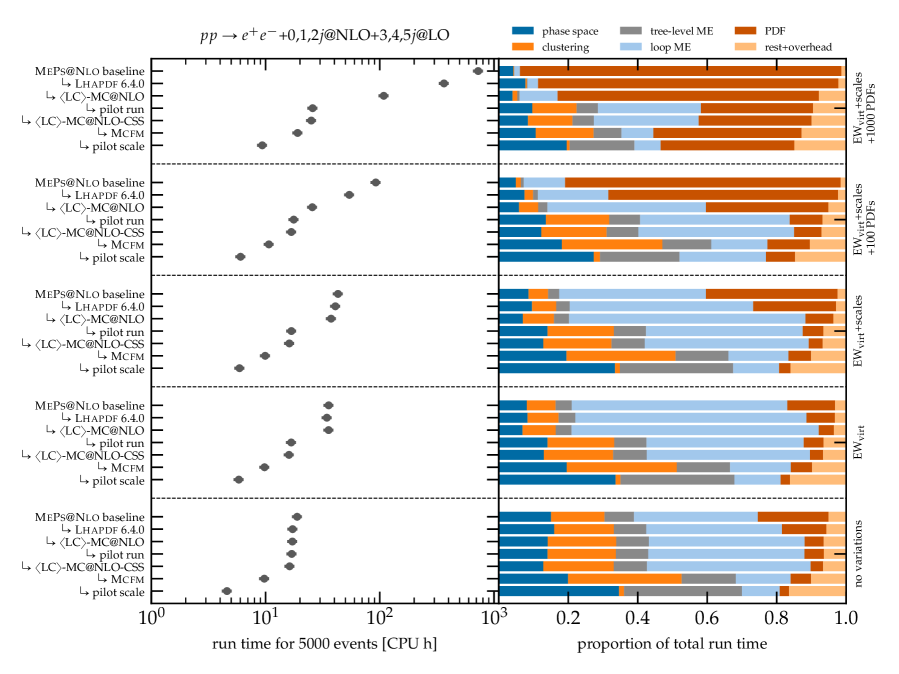
Figure 3: Reduction in overall run time for different performance improvements, combined with the breakdown of the overall run time into a high-level calculation composition. The timing is assessed by producing 5000 particle-level events for $pp\to e^{+}e^{-}+0,1,2j$@NLO${}+3,4,5j$@LO using M E P S @N LO . The scaling with the number of additional variation weights is benchmarked through a few representative setup configurations.

$pp\to e^{+}e^{-}+0,1,2j\text{@NLO}+3,4,5j\text{@LO}$.

We begin our analysis by examining the behaviour of the $e^{+}e^{-}+\text{jets}$ setup. Figure 3 shows the impact of each improvement on the total run time to generate 5000 unweighted events on the left side, and the composition of these run times for each of the seven steps, respectively, on the right side. For the total run times, horizontal error bars indicate a $10\text{\,}\mathrm{\char 37\relax}$ uncertainty estimate.

First, we note that using L HAPDF 6.4 reduces the overall run time by about $4050\text{\,}\mathrm{\char 37\relax}$ when many PDF variations are used, i.e. for the setup variants with 100 and 1000 PDF variations. Unsurprisingly, the proportion of total runtime dedicated to PDF evaluation shrinks accordingly.

The effect of additionally enabling $\langle\text{LC}\rangle$–M C @N LO scales with the number of PDF and scale variations, which also determines the number of required M C @N LO one-step shower variations required. Hence, for $\text{EW}_{\text{virt}}$+scales, it gives a speed-up of about $10\text{\,}\mathrm{\char 37\relax}$, while for the setup with 1000 PDF variations, more than a factor of three is gained.

The biggest impact (apart from the “no variations” setup variant) is achieved when also enabling the pilot run. It removes the overhead of calculating variations nearly entirely, such that the resulting runtimes are then very comparable across all setup variants. Only when calculating 1000 PDF variations there is still a sizeable increase of about $40\text{\,}\mathrm{\char 37\relax}$ in runtime, compared to the “no variations” variant.

Additionally moving the matched first shower emission into the normal cssshower simulation, $\langle\text{LC}\rangle$–M C @N LO –css, gives a speed-up of $510\text{\,}\mathrm{\char 37\relax}$ for all setup variants.

Then, switching to use M CFM for pre-unweighting loop calculations gives another sizeable reduction in runtime by about $80\text{\,}\mathrm{\char 37\relax}$. This reduction is only diluted somewhat in the 1000 PDF variation case, given the sizeable amount of time that is still dedicated to calculating variations of the unweighted events.

Lastly, we observe another $5060\text{\,}\mathrm{\char 37\relax}$ reduction of the required CPU time when choosing a scale definition that does not need to reconstruct the parton shower history to determine the factorisation and renormalisation scales of a candidate event in the pilot run. It has to be noted though that the correction to the proper CKKW factorisation and renormalisation scales induces a residual weight, i.e. a broader weight distribution, leading to a reduced statistical power of the resulting sample of the same number of events. We will discuss this further below.

The overall reduction in runtime for the setup variants is summed up in Tab. 1.

		$pp\to e^{+}e^{-}$ + jets				$pp\to t\bar{t}$ + jets
		runtime [CPU h/5k events]				runtime [CPU h/1k events]
setup variant		old	new	speed-up		old	new	speed-up
no variations		20 h	5 h	4$\times$		15 h	8 h	2$\times$
$\text{EW}_{\text{virt}}$		35 h	5 h	6$\times$		20 h	8 h	2$\times$
$\text{EW}_{\text{virt}}$+scales		45 h	5 h	7$\times$		25 h	8 h	4$\times$
$\text{EW}_{\text{virt}}$+scales+100 PDFs		90 h	5 h	15$\times$		55 h	8 h	7$\times$
$\text{EW}_{\text{virt}}$+scales+1000 PDFs		725 h	8 h	78$\times$		440 h	9 h	51$\times$

Table 1: Overall reduction in run time for all performance improvements combined. The timing is assessed by producing 5000 particle-level events for $pp\to e^{+}e^{-}+0,1,2j$@NLO${}+3,4,5j$@LO and 1000 particle-level events for $pp\to t\bar{t}+0,1j$@NLO${}+2,3,4j$@LO, both at M E P S @N LO . The scaling with the number of additional variation weights is benchmarked through a few representative setup configurations.

It is interesting to note that after applying all of the performance improvements, there is no longer a single overwhelmingly computationally intense component left in the composition shown in Fig. 3 (see the bottom line in each setup variant block): None of the components in the breakdown use more than $40\text{\,}\mathrm{\char 37\relax}$ of the runtime. With the exception of the 1000 PDF variation setup variant, the phase-space and tree-level ME components alone now require more than $50\text{\,}\mathrm{\char 37\relax}$ of the total runtime, such that they need to be targeted for further performance improvements. Also the virtual matrix elements (“loop ME”) are still sizeable (approximately $510\text{\,}\mathrm{\char 37\relax}$ of the runtime), albeit much smaller than the time spent on the remainder of the event generation. However, from the perspective of the S HERPA framework this is now irreducible as the runtime is spent in highly optimised external loop matrix-element libraries, and only when it is absolutely necessary.

$pp\to t\bar{t}+0,1j\text{@NLO}+2,3,4j\text{@LO}$

Following the analysis of the $e^{+}e^{-}+\text{jets}$ case, we now present the breakdown of $t\bar{t}+\text{jets}$ run times and their compositions in Fig. 4. Overall, the results are very similar. The most striking difference in the runtime decomposition is that the clustering part is about twice as large compared to the $e^{+}e^{-}+\text{jets}$ case. This is mainly related to the usage of a clustering-based scale definition in the $\mathbb{H}$-events, and also to the different structure of the core process. In the $t\bar{t}$ case, the initial state is dominated by gluons instead of quarks, and the core process comprises four partons instead of two. Therefore, there are considerably more ways to cluster a given jet configuration back into the core process. Secondly, we find that the loop matrix elements have a smaller relative footprint in the $t\bar{t}$ case, which is due to them only being calculated to NLO accuracy for up to one additional jet (as opposed to two additional jets in the $e^{+}e^{-}$ case).

The speed-ups by the performance improvements are similar, but the larger proportion of the clustering and the smaller proportion of the loop matrix elements results in the pilot run improvement and the analytic loop matrix element improvement having a smaller impact than in the $e^{+}e^{-}$ case. Using the pilot scale also has a smaller effect than in to the $e^{+}e^{-}$ case: the simulation of $\mathbb{H}$-events requires the clustering to determine the parton shower starting scale as a phase space boundary for their shower subtraction terms [74]. The large clustering component can only be removed if the $\mathbb{H}$-events are calculated using a dedicated clustering-independent scale definition, as is the case in the $e^{+}e^{-}$ setup. Overall, the final runtime improvements as reported in Tab. 1 are smaller than the ones for the $e^{+}e^{-}$ process, but still very sizeable.

The most notable deviation in the improvement pattern comes from switching to M CFM for the unweighting step, which only has a minor impact in the $t\bar{t}$ case. This is due to the fact that only the $t\bar{t}$ process is implemented in this library while the $t\bar{t}j$ process, which is much more costly, has to be taken from O PEN L OOPS throughout.

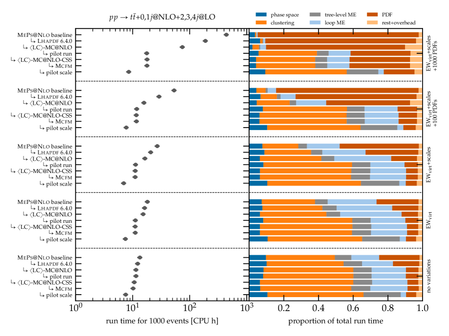
Figure 4: Reduction in overall run time for different performance improvements, combined with the breakdown of the overall run time into a high-level calculation composition. The timing is assessed by producing 1000 particle-level events for $pp\to t\bar{t}+0,1j$@NLO${}+2,3,4j$@LO using M E P S @N LO . The scaling with the number of additional variation weights is benchmarked through a few representative setup configurations.

Weight distribution for pilot scale

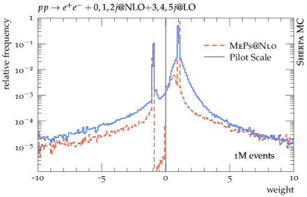
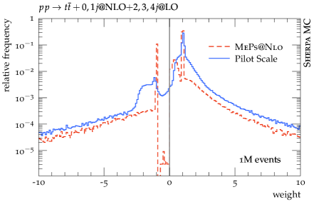
Figure 5: Weight distribution of events using either the default M E P S @N LO algorithm (red dashed) or the pilot scale strategy (blue solid) described in Sec. 4.

The remaining question is whether the pilot run strategy adversely affects the overall event weight. The large reduction in computing timing observed in the last steps in Figs. 3 and 4 would then be reduced by the unweighting efficiency in a second unweighting step that accounts for the mismatch between the scale definitions. Fig. 5 shows the weight distribution of events after the complete simulation, i.e. including the matching and merging procedure. We perform the analysis in partially unweighted mode, which implies that the event weight can be modified by local $K$-factors [74], and events are hence not fully unweighted. Note that the distributions are presented on a logarithmic scale. The average weights in the positive (negative) domain are 1.00 (-1.06) with a weight spread around 0.32 (0.52) when using the M E P S @N LO algorithm and 1.03 (-1.12) with a weight spread around 0.40 (0.83) when using the pilot scale strategy for $pp\to e^{+}e^{-}+0,1,2j$@NLO${}+3,4,5j$@LO. For $pp\to t\bar{t}+0,1j$@NLO${}+2,3,4j$@LO the average weights in the positive (negative) domain are 1.02 (-1.23) with a weight spread around 0.65 (0.98) when using the M E P S @N LO algorithm and 1.24 (-1.85) with a weight spread around 0.84 (1.59) when using the pilot scale strategy. The efficiency of a second unweighting step that would make the event sample unweighted can now be estimated as follows: Determine the number of events to be generated. This corresponds to the area under the curve, integrating from the top. Find the weight of the right (left) edge of the area integrated over in the positive (negative) half plane. The unweighting efficiency is the value of this weight (i.e. the maximum weight at the given number of events) divided by the average weight. Note that the average weight itself depends on the number of events. For a large number of events and a sharply peaked weight distribution, as in Fig. 5, this effect can be ignored. We find that the effective reduction in efficiency from using the pilot scale approach is typically less than a factor of two if the target number of events is large. The computing time reduction shown in the last steps in Figs. 3 and 4 will effectively be reduced by this amount, but the usage of a pilot scale is in most cases still beneficial.

Finally, Fig. 6 presents a cross-check between the M E P S @N LO method and the new pilot run strategy for actual $e^{+}e^{-}$ production physics observables given our $pp\to e^{+}e^{-}+0,1,2j$@NLO${}+3,4,5j$@LO setup. We show distributions which can already be defined at Born level ($m_{e^{+}e^{-}}$ and $y_{e^{+}e^{-}}$), as well as one observable which probes genuine higher-order effects ($p_{\mathrm{T}}^{e^{+}e^{-}}$). We observe agreement between the two scales at the statistical level, as well as MC uncertainties of the same magnitude. This indicates that our new pilot run strategy will be appropriate not only at the inclusive level, but also for fully differential event simulation. We have confirmed that the same conclusions are true for the $pp\to t\bar{t}+0,1j$@NLO${}+2,3,4j$@LO setup.

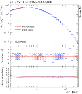
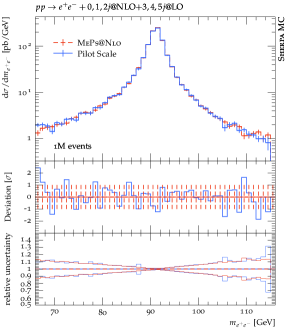
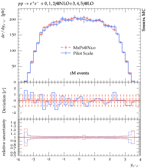
Figure 6: Predictions for the Born-level observables $m_{e^{+}e^{-}}$ and $y_{e^{+}e^{-}}$, and for the dilepton transverse momentum in comparison between the M E P S @N LO algorithm (red dashed) or the pilot scale strategy (blue solid) described in Sec. 4.

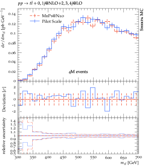
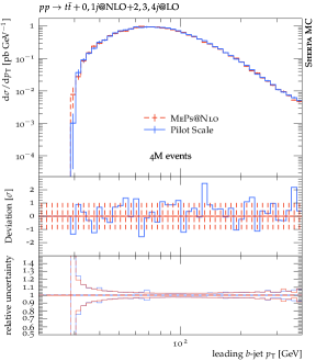
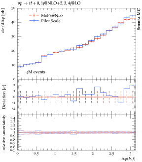
Figure 7: Predictions for the Born-level observable $m_{t\bar{t}}$, for the leading $b$-jet transverse momentum and the azimuthal difference between the leading $b$-jet and the leading light-flavour jet in comparison between the M E P S @N LO algorithm (red dashed) or the pilot scale strategy (blue solid) described in Sec. 4.

5 Future performance improvements

We have shown, that for a large number of PDF variations, L HAPDF still consumes a significant portion of the computing time. While current realistic setups are of roughly 100-200 variations, future analyses might require an ever increasing number of variations and thus again an improved L HAPDF and a better PDF call alignment in S HERPA .

The presented L HAPDF performance improvements mostly depend on better caching strategies. Future implementations might choose interpolators based on their ability to precompute and store computations. For example, switching from a 2-step local polynomial interpolator to a “proper” bicubic interpolation would allow to precompute all 16 coefficients of a third-order polynomial and only require a matrix-vector multiplication at run-time.

In the context of S HERPA in particular, with the increasing use of multi-weights in the Monte Carlo event generation, the next step to even further increase the caching of common computations would be to also cache the shared computations of the error sets. This requires all the variations to be evaluated at the same time, without changing the $(x,Q^{2})$ point before moving to the next one. This could be a further consideration if the number of variations increases but requires a restructuring of the call pattern in S HERPA .

However, currently for the realistic setups we presented, the majority of computing-time is spent on phase space and matrix element computations which would thus be the natural next step for performance improvements. In particular for the high multiplicity matrix elements the generation of unweighted events suffers from low unweighting efficiencies (which is also the reason why the pilot-run yields such significant improvements).

A comparison between S HERPA and M CFM suggested that this computing time can be further reduced [67]: Firstly, Sherpa could make use of the analytic tree-level matrix elements available in M CFM . Secondly, the phase-space integration strategy used by M CFM could be adopted by S HERPA in order to increase efficiency.

In addition to these more traditional techniques, high multiplicity matrix elements could be evaluated on GPUs, a path which has been charted in [78]. We expect significant improvements in this direction in the following years [4].

Finally, the improvements presented in Sec. 3.2 enable Sherpa to be used for the processing of the HDF5 event files introduced in [26], both at leading and at next-to-leading order precision. The corresponding technology is currently being implemented.

6 Conclusion

This manuscript discussed performance improvements of two major software packages needed for event generation at the High-Luminosity LHC: S HERPA and L HAPDF . We have presented multiple simple strategies to reduce the computing time needed for unweighted event generation in these two packages, while maintaining the formal precision of the computations. In combination, we achieve a reduction of a factor 15 (7) in the computing requirements for state-of-the-art $pp\to e^{+}e^{-}+0,1,2j$@NLO${}+3,4,5j$@LO ($pp\to t\bar{t}+0,1j$@NLO${}+2,3,4j$@LO) simulations at the LHC. With this, we have achieved a major milestone set by the HSF event generator working group and opened a path towards high-fidelity event simulation in the HL-LHC era. Our modifications are made publicly available for immediate use by the LHC experiments.

Appendix A Run cards

Listings 1 and 2 show the runcards used in this study for $Z+$jets and $t\bar{t}+$jets production, respectively. Therein, we omit for brevity Standard Model parameter specifications, which have no bearing on the findings of this study.

⬇ 1(run){ 2 # Collider setup 3 BEAM_1 2212; BEAM_ENERGY_1 6500.; 4 BEAM_2 2212; BEAM_ENERGY_2 6500.; 5 6 # PDF setup 7 USE_PDF_ALPHAS 1; 8 PDF_LIBRARY LHAPDFSherpa; 9 PDF_SET NNPDF30_nnlo_as_0118; 10 11 # ME generator settings 12 ME_SIGNAL_GENERATOR Comix Amegic LOOPGEN PILOTLGEN; 13 LOOPGEN:=OpenLoops; 14 PILOTLGEN:=MCFM; # analytic virtual corrs., see Sec. 3.3 15 16 # Tags for steering the process setup 17 NJET:=5; LJET:=2,3,4; QCUT:=20.; 18 19 # Scale definitions 20 SCALES PILOT{H_Tp2}{H_Tp2/sqr(2*max(1,N_FS-2))}; # simple pilot scale, see Sec. 3.4 21 PP_RS_SCALE VAR{H_Tp2/4}; 22 23 # Shower settings and neg. weight reduction 24 NLO_SUBTRACTION_SCHEME 2; 25 METS_BBAR_MODE 5; 26 NLO_CSS_PSMODE 2; # $\langle\text{LC}\rangle$-matching, see Sec. 3.1 27 PP_HPSMODE 0; 28 OVERWEIGHT_THRESHOLD 10; 29 30 # Variation setup 31 SCALE_VARIATIONS 0.25,0.25 0.25,1. 1.,0.25 1.,1. 1.,4. 4.,1. 4.,4.; 32 PDF_VARIATIONS NNPDF30_nnlo_as_0118_1000[all]; 33 ASSOCIATED_CONTRIBUTIONS_VARIATIONS EW EW|LO1; 34 35 # Parton-shower reweighting setup 36 CSS_REWEIGHT 1; 37 REWEIGHT_SPLITTING_PDF_SCALES 1; 38 REWEIGHT_SPLITTING_ALPHAS_SCALES 1; 39 40 # Model setup 41 EW_SCHEME 3; 42 OL_PARAMETERS ew_renorm_scheme 1; 43}(run) 44 45(processes){ 46 Process 93 93 -> 11 -11 93{NJET}; 47 Order (*,2); CKKW sqr(QCUT/E_CMS); 48 Enhance_Function VAR{max(pow(sqrt(H_T2)-PPerp(p[2])-PPerp(p[3]),2),PPerp2(p[2]+p[3]))/400.0} {3,4,5,6,7,8}; 49 Associated_Contributions EW|LO1 {LJET}; 50 NLO_QCD_Mode MC@NLO {LJET}; 51 ME_Generator Amegic {LJET}; 52 RS_ME_Generator Comix {LJET}; 53 Loop_Generator LOOPGEN {LJET}; 54 Pilot_Loop_Generator PILOTLGEN {LJET}; 55 Max_N_Quarks 4 {6,7,8}; 56 Max_Epsilon 0.01 {6,7,8}; 57 Integration_Error 0.99 {3,4,5,6,7,8}; 58 End process; 59}(processes) 60 61(selector){ 62 Mass 11 -11 40.0 E_CMS; 63}(selector) Listing 1: S HERPA runcard for $Z+$jets production, in the 1000 variations setup.

⬇ 1(run){ 2 # Collider setup 3 BEAM_1 2212; BEAM_ENERGY_1 6500.; 4 BEAM_2 2212; BEAM_ENERGY_2 6500.; 5 6 # PDF setup 7 USE_PDF_ALPHAS 1; 8 PDF_LIBRARY LHAPDFSherpa; 9 PDF_SET NNPDF30_nnlo_as_0118; 10 11 # ME generator settings 12 ME_SIGNAL_GENERATOR Comix Amegic LOOPGEN PILOTLGEN; 13 LOOPGEN:=OpenLoops; 14 PILOTLGEN:=MCFM; # analytic virtual corrs., see Sec. 3.3 15 16 # Tags for steering the process setup 17 NJET:=4; LJET:=2,3; QCUT:=30.; 18 19 # Scale definitions 20 SCALES PILOT{H_TM2}{H_TM2/sqr(2*max(1,N_FS-2))}; # simple pilot scale, see Sec. 3.4 21 CORE_SCALE QCD; 22 EXCLUSIVE_CLUSTER_MODE 1; 23 24 # Shower settings and neg. weight reduction 25 NLO_SUBTRACTION_SCHEME 2; 26 METS_BBAR_MODE 5; 27 NLO_CSS_PSMODE 2; # $\langle\text{LC}\rangle$-matching, see Sec. 3.1 28 PP_HPSMODE 0; 29 OVERWEIGHT_THRESHOLD 10; 30 31 # Variation setup 32 SCALE_VARIATIONS 0.25,0.25 0.25,1. 1.,0.25 1.,1. 1.,4. 4.,1. 4.,4.; 33 PDF_VARIATIONS NNPDF30_nnlo_as_0118_1000[all]; 34 ASSOCIATED_CONTRIBUTIONS_VARIATIONS EW EW|LO1; 35 36 # Parton-shower reweighting setup 37 CSS_REWEIGHT 1; 38 REWEIGHT_SPLITTING_PDF_SCALES 1; 39 REWEIGHT_SPLITTING_ALPHAS_SCALES 1; 40 41 # Model setup 42 EW_SCHEME 3; 43 OL_PARAMETERS ew_renorm_scheme 1; 44 45 # top and W decay setup 46 HARD_DECAYS On; 47 SOFT_SPIN_CORRELATIONS 1; 48 49 HDH_STATUS[24,2,-1] 2; HDH_STATUS[24,4,-3] 2; 50 HDH_STATUS[24,12,-11] 2; HDH_STATUS[24,14,-13] 2; HDH_STATUS[24,16,-15] 2; 51 HDH_STATUS[-24,-2,1] 2; HDH_STATUS[-24,-4,3] 2; 52 HDH_STATUS[-24,-12,11] 2; HDH_STATUS[-24,-14,13] 2; HDH_STATUS[-24,-16,15] 2; 53 STABLE[24] 0; STABLE[6] 0; WIDTH[6] 0; 54}(run) 55 56(processes){ 57 Process 93 93 -> 6 -6 93{NJET}; 58 Order (*,0); CKKW sqr(QCUT/E_CMS); 59 Enhance_Function VAR{pow(max(sqrt(H_T2)-PPerp(p[2])-PPerp(p[3]),(PPerp(p[2])+PPerp(p[3]))/2)/30.0,2)} {3,4,5,6} 60 Associated_Contributions EW|LO1 {LJET}; 61 NLO_QCD_Mode MC@NLO {LJET}; 62 ME_Generator Amegic {LJET}; 63 RS_ME_Generator Comix {LJET}; 64 Loop_Generator LOOPGEN {LJET}; 65 Pilot_Loop_Generator PILOTLGEN {2}; 66 End process; 67}(processes) Listing 2: S HERPA runcard for $t\bar{t}+$jets production, in the 1000 variations setup.

References

- [1] T. Sjöstrand, The Lund Monte Carlo for Jet Fragmentation, Comput. Phys. Commun. 27 (1982), 243.
- [2] B. R. Webber, A QCD model for jet fragmentation including soft gluon interference, Nucl. Phys. B238 (1984), 492.
- [3] A. Buckley et al., General-purpose event generators for LHC physics, Phys. Rept. 504 (2011), 145–233, [arXiv:1101.2599 [hep-ph]].
- [4] J. M. Campbell et al., Event Generators for High-Energy Physics Experiments, arXiv:2203.11110 [hep-ph].
- [5] I. Zurbano Fernandez et al., High-Luminosity Large Hadron Collider (HL-LHC): Technical design report.
- [6] A. Buckley, Computational challenges for MC event generation, J. Phys. Conf. Ser. 1525 (2020), no. 1, 012023, [arXiv:1908.00167 [hep-ph]].
- [7] S. Amoroso et al., HSF Physics Event Generator WG collaboration, Challenges in Monte Carlo Event Generator Software for High-Luminosity LHC, Comput. Softw. Big Sci. 5 (2021), no. 1, 12, [arXiv:2004.13687 [hep-ph]].
- [8] HSF Physics Event Generator WG, HSF Physics Event Generator WG collaboration, HL-LHC Computing Review Stage-2, Common Software Projects: Event Generators, arXiv:2109.14938 [hep-ph].
- [9] T. Aarrestad et al., HL-LHC Computing Review: Common Tools and Community Software, 2022 Snowmass Summer Study (P. Canal et al., Eds.), 8 2020.
- [10] F. Krauss, R. Kuhn and G. Soff, AMEGIC++ 1.0: A Matrix Element Generator In C++, JHEP 02 (2002), 044, [hep-ph/0109036].
- [11] M. L. Mangano, M. Moretti, F. Piccinini, R. Pittau and A. D. Polosa, ALPGEN, a generator for hard multiparton processes in hadronic collisions, JHEP 07 (2003), 001, [hep-ph/0206293].
- [12] A. Cafarella, C. G. Papadopoulos and M. Worek, Helac-Phegas: A generator for all parton level processes, Comput. Phys. Commun. 180 (2009), 1941–1955, [arXiv:0710.2427 [hep-ph]].
- [13] T. Gleisberg and S. Höche, Comix, a new matrix element generator, JHEP 12 (2008), 039, [arXiv:0808.3674 [hep-ph]].
- [14] J. Alwall, M. Herquet, F. Maltoni, O. Mattelaer and T. Stelzer, MadGraph 5 : Going Beyond, JHEP 06 (2011), 128, [arXiv:1106.0522 [hep-ph]].
- [15] C. F. Berger, Z. Bern, L. J. Dixon, F. Febres Cordero, D. Forde, H. Ita, D. A. Kosower and D. Maître, An Automated Implementation of On-Shell Methods for One-Loop Amplitudes, Phys. Rev. D 78 (2008), 036003, [arXiv:0803.4180 [hep-ph]].
- [16] G. Cullen, N. Greiner, G. Heinrich, G. Luisoni, P. Mastrolia, G. Ossola, T. Reiter and F. Tramontano, Automated One-Loop Calculations with GoSam, Eur.Phys.J. C72 (2012), 1889, [arXiv:1111.2034 [hep-ph]].
- [17] G. Bevilacqua, M. Czakon, M. Garzelli, A. van Hameren, A. Kardos et al., HELAC-NLO, Comput.Phys.Commun. 184 (2013), 986–997, [arXiv:1110.1499 [hep-ph]].
- [18] F. Cascioli, P. Maierhöfer and S. Pozzorini, Scattering Amplitudes with Open Loops, Phys.Rev.Lett. 108 (2012), 111601, [arXiv:1111.5206 [hep-ph]].
- [19] J. Alwall, R. Frederix, S. Frixione, V. Hirschi, F. Maltoni, O. Mattelaer, H. S. Shao, T. Stelzer, P. Torrielli and M. Zaro, The automated computation of tree-level and next-to-leading order differential cross sections, and their matching to parton shower simulations, JHEP 07 (2014), 079, [arXiv:1405.0301 [hep-ph]].
- [20] S. Actis, A. Denner, L. Hofer, J.-N. Lang, A. Scharf and S. Uccirati, RECOLA: REcursive Computation of One-Loop Amplitudes, Comput. Phys. Commun. 214 (2017), 140–173, [arXiv:1605.01090 [hep-ph]].
- [21] K. Danziger, T. Janßen, S. Schumann and F. Siegert, Accelerating Monte Carlo event generation – rejection sampling using neural network event-weight estimates, arXiv:2109.11964 [hep-ph].
- [22] R. Frederix, S. Frixione, S. Prestel and P. Torrielli, On the reduction of negative weights in MC@NLO-type matching procedures, JHEP 07 (2020), 238, [arXiv:2002.12716 [hep-ph]].
- [23] K. Danziger, S. Höche and F. Siegert, Reducing negative weights in Monte Carlo event generation with Sherpa, arXiv:2110.15211 [hep-ph].
- [24] J. R. Andersen, C. Gütschow, A. Maier and S. Prestel, A Positive Resampler for Monte Carlo events with negative weights, Eur. Phys. J. C 80 (2020), no. 11, 1007, [arXiv:2005.09375 [hep-ph]].
- [25] B. Nachman and J. Thaler, Neural resampler for Monte Carlo reweighting with preserved uncertainties, Phys. Rev. D 102 (2020), no. 7, 076004, [arXiv:2007.11586 [hep-ph]].
- [26] S. Höche, S. Prestel and H. Schulz, Simulation of Vector Boson Plus Many Jet Final States at the High Luminosity LHC, Phys. Rev. D 100 (2019), no. 1, 014024, [arXiv:1905.05120 [hep-ph]].
- [27] E. Bothmann et al., Sherpa collaboration, Event Generation with Sherpa 2.2, SciPost Phys. 7 (2019), no. 3, 034, [arXiv:1905.09127 [hep-ph]].
- [28] A. Buckley, J. Ferrando, S. Lloyd, K. Nordström, B. Page, M. Rüfenacht, M. Schönherr and G. Watt, LHAPDF6: parton density access in the LHC precision era, Eur. Phys. J. C75 (2015), 132, [arXiv:1412.7420 [hep-ph]].
- [29] G. Aad et al., ATLAS collaboration, Modelling and computational improvements to the simulation of single vector-boson plus jet processes for the ATLAS experiment, arXiv:2112.09588 [hep-ex].
- [30] Y. L. Dokshitzer, Calculation of the structure functions for deep inelastic scattering and annihilation by perturbation theory in quantum chromodynamics, Sov. Phys. JETP 46 (1977), 641–653.
- [31] V. N. Gribov and L. N. Lipatov, Deep inelastic - scattering in perturbation theory, Sov. J. Nucl. Phys. 15 (1972), 438–450.
- [32] L. N. Lipatov, The parton model and perturbation theory, Sov. J. Nucl. Phys. 20 (1975), 94–102.
- [33] G. Altarelli and G. Parisi, Asymptotic freedom in parton language, Nucl. Phys. B126 (1977), 298–318.
- [34] T. Sjöstrand, A model for initial state parton showers, Phys. Lett. B157 (1985), 321.
- [35] R. K. Ellis, W. J. Stirling and B. R. Webber, QCD and collider physics, vol. 8, Cambridge University Press, 2 2011.
- [36] W. H. Press, S. A. Teukolsky, W. T. Vetterling and B. P. Flannery, Numerical Recipes in C, ed. second, Cambridge University Press, Cambridge, USA, 1992.
- [37] E. Bothmann et al., Sherpa collaboration, Event Generation with Sherpa 2.2, SciPost Phys. 7 (2019), no. 3, 034, [arXiv:1905.09127 [hep-ph]].
- [38] F. Buccioni, J.-N. Lang, J. M. Lindert, P. Maierhöfer, S. Pozzorini, H. Zhang and M. F. Zoller, OpenLoops 2, Eur. Phys. J. C 79 (2019), no. 10, 866, [arXiv:1907.13071 [hep-ph]].
- [39] T. Gleisberg and F. Krauss, Automating dipole subtraction for QCD NLO calculations, Eur. Phys. J. C53 (2008), 501–523, [arXiv:0709.2881 [hep-ph]].
- [40] S. Schumann and F. Krauss, A parton shower algorithm based on Catani-Seymour dipole factorisation, JHEP 03 (2008), 038, [arXiv:0709.1027 [hep-ph]].
- [41] S. Höche, F. Krauss, M. Schönherr and F. Siegert, A critical appraisal of NLO+PS matching methods, JHEP 09 (2012), 049, [arXiv:1111.1220 [hep-ph]].
- [42] S. Höche and M. Schönherr, Uncertainties in next-to-leading order plus parton shower matched simulations of inclusive jet and dijet production, Phys.Rev. D86 (2012), 094042, [arXiv:1208.2815 [hep-ph]].
- [43] S. Frixione and B. R. Webber, Matching NLO QCD computations and parton shower simulations, JHEP 06 (2002), 029, [hep-ph/0204244].
- [44] S. Kallweit, J. M. Lindert, P. Maierhöfer, S. Pozzorini and M. Schönherr, NLO QCD+EW predictions for V + jets including off-shell vector-boson decays and multijet merging, JHEP 04 (2016), 021, [arXiv:1511.08692 [hep-ph]].
- [45] S. Bräuer, A. Denner, M. Pellen, M. Schönherr and S. Schumann, Fixed-order and merged parton-shower predictions for WW and WWj production at the LHC including NLO QCD and EW corrections, JHEP 10 (2020), 159, [arXiv:2005.12128 [hep-ph]].
- [46] E. Bothmann, M. Schönherr and S. Schumann, Reweighting QCD matrix-element and parton-shower calculations, Eur. Phys. J. C76 (2016), no. 11, 590, [arXiv:1606.08753 [hep-ph]].
- [47] B. Gregg, FlameGraph, 2011.
- [48] A. Bassetto, M. Ciafaloni and G. Marchesini, Jet structure and infrared sensitive quantities in perturbative QCD, Phys. Rept. 100 (1983), 201–272.
- [49] S. Höche, S. Schumann and F. Siegert, Hard photon production and matrix-element parton-shower merging, Phys. Rev. D81 (2010), 034026, [arXiv:0912.3501 [hep-ph]].
- [50] C. F. Berger, Z. Bern, L. J. Dixon, F. Febres-Cordero, D. Forde, T. Gleisberg, H. Ita, D. A. Kosower and D. Maître, Next-to-leading order QCD predictions for W+3-Jet distributions at hadron colliders, Phys. Rev. D80 (2009), 074036, [arXiv:0907.1984 [hep-ph]].
- [51] C. F. Berger, Z. Bern, L. J. Dixon, F. Febres-Cordero, D. Forde, T. Gleisberg, H. Ita, D. A. Kosower and D. Maître, Next-to-leading order QCD predictions for +3-Jet distributions at the Tevatron, Phys. Rev. D82 (2010), 074002, [arXiv:1004.1659 [hep-ph]].
- [52] C. F. Berger, Z. Bern, L. J. Dixon, F. Febres-Cordero, D. Forde, T. Gleisberg, H. Ita, D. A. Kosower and D. Maître, Precise Predictions for W + 4-Jet Production at the Large Hadron Collider, Phys. Rev. Lett. 106 (2011), 092001, [arXiv:1009.2338 [hep-ph]].
- [53] H. Ita, Z. Bern, L. J. Dixon, F. Febres-Cordero, D. A. Kosower and D. Maître, Precise Predictions for Z + 4 Jets at Hadron Colliders, Phys.Rev. D85 (2012), 031501, [arXiv:1108.2229 [hep-ph]].
- [54] Z. Bern, L. Dixon, F. Febres Cordero, S. Höche, H. Ita, D. A. Kosower, D. Maître and K. J. Ozeren, Next-to-Leading Order -Jet Production at the LHC, Phys.Rev. D88 (2013), 014025, [arXiv:1304.1253 [hep-ph]].
- [55] V. Hirschi, R. Frederix, S. Frixione, M. V. Garzelli, F. Maltoni and R. Pittau, Automation of one-loop QCD corrections, JHEP 05 (2011), 044, [arXiv:1103.0621 [hep-ph]].
- [56] F. Buccioni, S. Pozzorini and M. Zoller, On-the-fly reduction of open loops, Eur. Phys. J. C 78 (2018), no. 1, 70, [arXiv:1710.11452 [hep-ph]].
- [57] S. Badger, B. Biedermann and P. Uwer, NGluon: A Package to Calculate One-loop Multi-gluon Amplitudes, Comput.Phys.Commun. 182 (2011), 1674–1692, [arXiv:1011.2900 [hep-ph]].
- [58] S. Badger, B. Biedermann, P. Uwer and V. Yundin, Numerical evaluation of virtual corrections to multi-jet production in massless QCD, Comput.Phys.Commun. 184 (2013), 1981–1998, [arXiv:1209.0100 [hep-ph]].
- [59] G. Cullen, H. van Deurzen, N. Greiner, G. Heinrich, G. Luisoni et al., GOSAM-2.0: a tool for automated one-loop calculations within the Standard Model and beyond, Eur.Phys.J. C74 (2014), no. 8, 3001, [arXiv:1404.7096 [hep-ph]].
- [60] S. Actis, A. Denner, L. Hofer, A. Scharf and S. Uccirati, Recursive generation of one-loop amplitudes in the Standard Model, JHEP 04 (2013), 037, [arXiv:1211.6316 [hep-ph]].
- [61] A. Denner, J.-N. Lang and S. Uccirati, NLO electroweak corrections in extended Higgs Sectors with RECOLA2, JHEP 07 (2017), 087, [arXiv:1705.06053 [hep-ph]].
- [62] A. Denner, J.-N. Lang and S. Uccirati, Recola2: REcursive Computation of One-Loop Amplitudes 2, Comput. Phys. Commun. 224 (2018), 346–361, [arXiv:1711.07388 [hep-ph]].
- [63] J. M. Campbell and R. K. Ellis, Update on vector boson pair production at hadron colliders, Phys. Rev. D60 (1999), 113006, [hep-ph/9905386].
- [64] J. M. Campbell, R. K. Ellis and C. Williams, Vector boson pair production at the LHC, JHEP 07 (2011), 018, [arXiv:1105.0020 [hep-ph]].
- [65] J. M. Campbell, R. K. Ellis and W. T. Giele, A Multi-Threaded Version of MCFM, arXiv:1503.06182 [physics.comp-ph].
- [66] J. Campbell and T. Neumann, Precision Phenomenology with MCFM, JHEP 12 (2019), 034, [arXiv:1909.09117 [hep-ph]].
- [67] J. M. Campbell, S. Höche and C. T. Preuss, Accelerating LHC phenomenology with analytic one-loop amplitudes: A C++ interface to MCFM, Eur. Phys. J. C 81 (2021), 1117, [arXiv:2107.04472 [hep-ph]].
- [68] T. Binoth et al., A proposal for a standard interface between Monte Carlo tools and one-loop programs, Comput. Phys. Commun. 181 (2010), 1612–1622, [arXiv:1001.1307 [hep-ph]].
- [69] S. Alioli, S. Badger, J. Bellm, B. Biedermann, F. Boudjema et al., Update of the Binoth Les Houches Accord for a standard interface between Monte Carlo tools and one-loop programs, Comput.Phys.Commun. 185 (2014), 560–571, [arXiv:1308.3462 [hep-ph]].
- [70] S. Catani, F. Krauss, R. Kuhn and B. R. Webber, QCD matrix elements + parton showers, JHEP 11 (2001), 063, [hep-ph/0109231].
- [71] L. Lönnblad, Correcting the colour-dipole cascade model with fixed order matrix elements, JHEP 05 (2002), 046, [hep-ph/0112284].
- [72] J. André and T. Sjöstrand, Matching of matrix elements and parton showers, Phys. Rev. D57 (1998), 5767–5772, [hep-ph/9708390].
- [73] D. Amati, A. Bassetto, M. Ciafaloni, G. Marchesini and G. Veneziano, A treatment of hard processes sensitive to the infrared structure of QCD, Nucl. Phys. B173 (1980), 429.
- [74] S. Höche, F. Krauss, M. Schönherr and F. Siegert, QCD matrix elements + parton showers: The NLO case, JHEP 04 (2013), 027, [arXiv:1207.5030 [hep-ph]].
- [75] T. Gehrmann, S. Höche, F. Krauss, M. Schönherr and F. Siegert, NLO QCD matrix elements + parton showers in hadrons, JHEP 01 (2013), 144, [arXiv:1207.5031 [hep-ph]].
- [76] S. Höche, F. Krauss, S. Pozzorini, M. Schönherr, J. Thompson, S. Pozzorini and K. C. Zapp, Triple vector boson production through Higgs-Strahlung with NLO multijet merging, Phys.Rev. D89 (2014), 093015, [arXiv:1403.7516 [hep-ph]].
- [77] R. D. Ball et al., NNPDF collaboration, Parton distributions for the LHC Run II, JHEP 04 (2015), 040, [arXiv:1410.8849 [hep-ph]].
- [78] E. Bothmann, W. Giele, S. Höche, J. Isaacson and M. Knobbe, Many-gluon tree amplitudes on modern GPUs: A case study for novel event generators, arXiv:2106.06507 [hep-ph].
- [79] A. Basden, M. Weinzierl, T. Weinzierl and B. J. N. Wylie, A novel performance analysis workshop series concept, developed at Durham University under the umbrella of the ExCALIBUR programme, August 2021.