On the reduction of negative weights in MC@NLO-type matching procedures

Abstract

We show how a careful analysis of the behaviour of a parton shower Monte Carlo in the vicinity of the soft and collinear regions allows one to formulate a modified MC@NLO-matching prescription that reduces the number of negative-weight events with respect to that stemming from the standard MC@NLO procedure. As a first practical application of such a prescription, that we dub MC@NLO-$\Delta$, we have implemented it in the MadGraph5_aMC@NLO framework, by employing the Pythia8 Monte Carlo. We present selected MC@NLO-$\Delta$ results at the 13 TeV LHC, and compare them with MC@NLO ones. We find that the former predictions are consistent with the latter ones within the typical matching systematics, and that the reduction of negative-weight events is significant.

1 Introduction

It is inconceivable that modern experimental high-energy particle physics be done without the massive use of event generators, which are also enjoying an increasing number of applications in theoretical phenomenology. This has stimulated a vigorous research activity in the past two decades, the upshot of which is that event generators, while maintaining their traditional flexibility, have significantly increased their predictive power (and its most important spinoff, the reduction of systematics), through matching and merging with perturbative matrix-element computations. Apart from a few selected cases, matching and merging are either carried out at the tree level or at the next-to-leading order (NLO). In this work, we shall consider only the latter simulations, that are more accurate than the former, but require more involved computations (which nowadays can fortunately be automated). On top of that, one must bear in mind that NLO cross sections are not positive-definite locally in the phase space. This implies that some of the hard events that will eventually be showered have negative weights. It is convenient to introduce an efficiency associated with the fraction of negative weights; denoting the latter by $f$, such an efficiency is defined as follows:

$$\varepsilon(f)=1-2f\,,\;\;\;\;\;\;\;\;0\leq f<0.5\;\;\;\;\;\;\Longrightarrow\;\;\;\;\;\;0<\varepsilon(f)\leq 1\,.$$ (1)

This efficiency stems from matrix-element computations (see e.g. eq. (4.33) of ref. Frixione:2002ik ), but it affects the overall performance of the latter only insofar that it is correlated with other efficiencies relevant to them; for example, it is usually the case that phase-space integration converges slightly faster in the case of a positive-definite integrand than in the case of an integrand whose sign can change; similar considerations are valid e.g. for the unweighting efficiency. However, for all practical purposes such correlations can be neglected: by far, the most significant impact of $\varepsilon(f)$ being smaller than one is that it implies that, in order to obtain the same statistical accuracy at the level of physical observables as the one of a positive-definite simulation, a number of events must be generated which is larger than in the latter case. In order to quantify this statement, let us denote by:

$$N\,,\;\;\;\;\;\;\;\;N_{+}=(1-f)N\,,\;\;\;\;\;\;\;\;N_{-}=fN\;\;\;\;\;\;\Longrightarrow\;\;\;\;\;\;N=N_{+}+N_{-}\,,$$ (2)

the total number of events, the number of events with positive weights, and the number of events with negative weights, respectively. Furthermore, we assume such events to be unweighted: in other words, their weights are equal to $\pm\omega$, with $\omega>0$ a factor that is constant for all events in a given generation and that includes the suitable normalisation. The resulting cross section and its associated error will thus be:

$$\sigma = \omega\left(N_{+}-N_{-}\pm\sqrt{N_{+}+N_{-}+2C_{\pm}\sqrt{N_{+}}\sqrt{N_{-}}}\right)$$ (3)

$$= \omega\left(\varepsilon(f)N\pm\sqrt{1+C_{\pm}\sqrt{1-\varepsilon(f)^{2}}}\sqrt{N}\right),$$

where by $C_{\pm}$ we have denoted the non-negative correlation between positive- and negative-weight events (this number is typically neglected). In the context of a positive-definite simulation, where $M$ unweighted events are generated with weights all equal to $\omega^{\prime}>0$, the analogue of eq. (3) reads:

$$\sigma=\omega^{\prime}\left(M\pm\sqrt{M}\right).$$ (4)

By imposing the cross sections in eqs. (3) and (4) to have the same relative error we obtain:

$$N=c(f)\,M\,,$$ (5)

where

$$c(f)=\frac{1+C_{\pm}\sqrt{1-\varepsilon(f)^{2}}}{\varepsilon(f)^{2}}\,.$$ (6)

The fact that $N\geq M$ (with $N=M$ if and only if $f=0$) formalises what was stated before eq. (2): a simulation that features events of either sign can attain the same statistical accuracy as one that is positive definite only by generating a number of events which is larger by a factor $c(f)$ w.r.t. that of the latter. For this reason, we call $c(f)$ the relative cost of the simulation; we plot this quantity as a function of $f$ in fig. 1, for $C_{\pm}=0,0.5,1$.

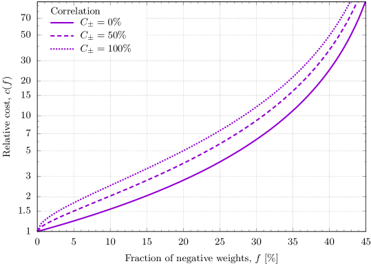
Figure 1: Relative cost as a function of the fraction of negative weights, eq. (6), for three different values of the correlation parameter $C_{\pm}$.

The discussion thus far has been rather schematic. For example, we have implicitly assumed $f$ to be independent of the kinematics, which is never the case. More correctly, one would need to use eqs. (3) and (4) locally in the phase space, thus defining a local relative cost, and subsequently construct the global relative cost as the weighted (by number of events) average of the local ones. In practice, eq. (6), with $f$ the overall fraction of negative-weight events, does characterise well enough the behaviour of simulations with events of either sign, and we shall often use it in the following.

The problem with $c(f)>1$ for any $f>0$ is not statistics per se, but the fact that it generally implies additional financial costs: longer running times, hence larger power consumption (events with negative weights contribute to climate change!), and bigger storage space, to name just the most important ones. Denoting by $p$ ($p^{\prime}$) the overall price tag for the generation, full simulation, analysis, and storage of an individual event resulting from a positive-definite (non-positive-definite) simulation, the additional costs alluded to before are:

$$Np^{\prime}-Mp=M\,\big{[}c(f)p^{\prime}-p\big{]}\,.$$ (7)

With all other things being equal (and chiefly among them, the control of the theoretical systematics), it is therefore advantageous to make $f$ as small as possible, so as to minimise the additional costs of eq. (7). This is the goal of the present work, in the context of the MC@NLO matching formalism Frixione:2002ik .

Before proceeding, we remind the reader that currently the vast majority of theoretical studies, and essentially all of the NLO$+$parton shower simulations performed by experimental collaborations, are based on either the MC@NLO or the POWHEG Nason:2004rx methods, and on their closely-related variants Hoeche:2011fd ; Platzer:2011bc ; alternative approaches (see e.g. refs. Nagy:2005aa ; Bauer:2006mk ; Nagy:2007ty ; Giele:2007di ; Bauer:2008qh ; Jadach:2015mza ) are much less well-developed, and rarely used in practice. At variance with MC@NLO, the POWHEG formalism is characterised by a very small fraction of negative weights. Such an appealing feature relies, among other things, on the exponentiation of real-emission matrix elements. This induces a few characteristic features, in particular because neither these matrix elements nor their associated phase spaces exponentiate away from the soft and collinear regions. If we denote by $\alpha_{\scriptscriptstyle S}^{b}$ the Born-level perturbative order relevant to a given computation, at ${\cal O}(\alpha_{\scriptscriptstyle S}^{b+2})$ (and beyond) the POWHEG physical prediction will contain potentially large terms whose origin is due to matrix elements of ${\cal O}(\alpha_{\scriptscriptstyle S}^{b+1})$, in addition to those naturally resulting from Monte-Carlo (MC henceforth) parton showers. This is avoided by construction in the MC@NLO matching, where all terms of ${\cal O}(\alpha_{\scriptscriptstyle S}^{b+2})$ and beyond are solely of MC origin.

The central idea of the present work is that of showing that, by a suitable modification of the ${\cal O}(\alpha_{\scriptscriptstyle S}^{k})$ terms ($k\geq 2$) in an MC@NLO cross section by means of contributions of sole MC origin, one arrives at a matching prescription, that we call MC@NLO-$\Delta$, which preserves the good features of MC@NLO while significantly reducing the fraction of negative weights. In particular, the formal ${\cal O}(\alpha_{\scriptscriptstyle S}^{b+1})$ expansion of the MC@NLO-$\Delta$ cross section coincides with that of MC@NLO and hence, by construction, with the NLO result. In the infrared regions, the logarithmic behaviour of MC@NLO-$\Delta$ is the same as that of the MC one matches to, as is the case for MC@NLO. Furthermore, the MC@NLO-$\Delta$ formulation leads in a natural manner to a richer structure of the hard events to be showered by the MC. Namely, a (generally different) shower scale is associated with each oriented colour line, and is passed to the MC; this is in contrast to what is done currently, where a single scale characterises the production process, and is regarded as a global property of the event. Finally, we note that in NLO-matched MCs the fraction of negative-weight events with Born kinematics can be reduced by means of a procedure that has been called folding in ref. Nason:2007vt , and implemented in practice in POWHEG in ref. Alioli:2010xd . Here we shall show that, on top of the intrinsic reduction of the number of negative-weight events in the MC@NLO-$\Delta$ matching, the folding technique is rather effective there, whereby such a reduction is more pronounced than in the case of the standard MC@NLO matching.

This paper is organised as follows. In sect. 2 we review the basic properties of the MC@NLO matching that lead to negative-weight events, and classify the latter. In sect. 3 we introduce the new matching prescription, MC@NLO-$\Delta$, that constitutes the core of this work. This is based on a scalar quantity, $\Delta$, whose construction we describe in detail in sect. 3.1; the hard-event multi-scale structure it induces is introduced in sect. 3.2. Some peculiar features of the practical implementation of MC@NLO-$\Delta$ are reported in sect. 4. In sect. 5 we present sample hadroproduction MC@NLO-$\Delta$ results, which we systematically compare with their MC@NLO counterparts. We draw our conclusions in sect. 6. Finally, some technical information on the Pythia8 Sudakov form factors are collected in appendix A.

2 Anatomy of negative weights in MC@NLO

We start by pointing out that in MC@NLO the exact amount of negative-weight events and their distribution in the phase space depend on several elements. Among these, the most important are the following: the parton shower MC one matches to, and in particular its shower variables; the technique, which is typically a subtraction procedure, used to compute the underlying NLO cross section; and the choice of the phase-space parametrisation employed in the latter computation. Therefore, in a bottom-up approach to the reduction of negative weights, one would construct the shower and the short-distance computations with the specific goal of minimising $f$. This is a potentially very interesting strategy, which however appears to be quite complicated; we shall not pursue it here. Rather, we shall follow a top-down approach, where both the shower and the NLO calculations are considered as given, and it is the matching between them which is responsible for the minimisation of $f$. This can be done thanks to the fact that, in spite of their specific features mentioned above, negative weights possess universal characteristics which one can exploit to reduce their number. In order to discuss such universal characteristics, we now sketch out the basic MC@NLO formulae, simplifying them as much as possible, lest the details obscure the basic ideas. If the reader wants to be definite, explicit expressions based on FKS subtraction Frixione:1995ms ; Frixione:1997np can be found e.g. in refs. Frederix:2009yq ; Alwall:2014hca ; Frederix:2018nkq for the MadGraph5_aMC@NLO implementation (MG5_aMC henceforth).

The key simplification from a notational viewpoint stems from one of the basic features of the FKS subtraction and of the MC@NLO implementations based on it. Namely, for any given real-emission process the phase space is partitioned in an effective manner by means of the ${\cal S}$ functions, so that one ultimately deals with a linear combination of short-distance cross sections which have, at most, one soft and one collinear singularity. Such a partition singles out two partons, called the FKS parton and its sister, with which the soft and collinear singularities are associated. We shall thus work by using the rule:

• The following formulae assume that the real-emission process, the FKS parton (labelled by $i$), and the sister of the latter (labelled by $j$) are given and fixed. In order to obtain the physical cross sections, one must sum over these quantities.

Bearing the above condition in mind, the MC@NLO generating functional is written as follows:

$${\cal F}_{\mbox{\tiny MC@NLO}}={\cal F}_{\mbox{\tiny MC}}\!\left({\cal K}^{({\mathbb{H}})}\right)d\sigma^{\scriptscriptstyle({\mathbb{H}})}+{\cal F}_{\mbox{\tiny MC}}\!\left({\cal K}^{({\mathbb{S}})}\right)d\sigma^{\scriptscriptstyle({\mathbb{S}})}\,,$$ (8)

where ${\cal F}_{\mbox{\tiny MC}}$ is the generating functional of the MC one matches to. By ${\cal K}^{({\mathbb{H}})}$ and ${\cal K}^{({\mathbb{S}})}$ we have denoted ${\mathbb{H}}$- and ${\mathbb{S}}$-event kinematic configurations, respectively. For example, if Born-level processes for the cross section of interest feature $n$ final-state particles, ${\cal K}^{({\mathbb{H}})}$ and ${\cal K}^{({\mathbb{S}})}$ correspond to $2\to n+1$ and $2\to n$ configurations, respectively. The short-distance cross sections on the r.h.s. of eq. (8) are:

$$d\sigma^{\scriptscriptstyle({\mathbb{H}})} = d\sigma^{\scriptscriptstyle{(\rm NLO},E)}-d\sigma^{\scriptscriptstyle\rm(MC)}\,,$$ (9)

$$d\sigma^{\scriptscriptstyle({\mathbb{S}})} = d\sigma^{\scriptscriptstyle\rm(MC)}+\sum_{\alpha=S,C,SC}d\sigma^{{\scriptscriptstyle(\rm NLO},\alpha{\scriptscriptstyle)}}\,.$$ (10)

Here, we have denoted by $d\sigma^{\scriptscriptstyle\rm(MC)}$ the MC counterterms; the other contributions are identical to those that enter an NLO fixed-order cross section:

$$\frac{d\sigma^{\scriptscriptstyle\rm(NLO)}}{d{\cal K}}=\delta\!\left({\cal K}-{\cal K}^{({\mathbb{H}})}\right)d\sigma^{\scriptscriptstyle{(\rm NLO},E)}+\delta\!\left({\cal K}-{\cal K}^{({\mathbb{S}})}\right)\sum_{\alpha=S,C,SC}d\sigma^{{\scriptscriptstyle(\rm NLO},\alpha{\scriptscriptstyle)}}\,.$$ (11)

Thus, $d\sigma^{\scriptscriptstyle{(\rm NLO},E)}$ is the real-emission contribution, while $d\sigma^{{\scriptscriptstyle(\rm NLO},\alpha{\scriptscriptstyle)}}$, $\alpha=S,C,SC$ collect all of the other terms (the Born, and contributions of virtual, soft, collinear, and soft-collinear origin; in a non-FKS language, the latter are therefore the integrated and unintegrated fixed-order counterterms). We point out that the cross sections on the r.h.s. of eqs. (9) and (10) have support in an $(n+1)$-body phase space. We write the latter as follows:

$$d\phi_{n+1}=\Phi^{(n+1)}\left(\chi_{n+1}\right)\,d\chi_{n+1}\,,$$ (12)

where $\chi_{n+1}$ denotes the set of the chosen $3n-1$ integration variables, whose nature need not be specified here, except for the fact that its has the following general form:

$$\chi_{n+1} = \chi_{n}\bigcup\chi_{r}\,,$$ (13)

$$\chi_{r} = \big{\{}\xi,y,\varphi\big{\}}\,.$$ (14)

By $\chi_{n}$ we have denoted $3n-4$ integration variables that define $n$-body (i.e. Born-level) configurations, and by $\chi_{r}$ the variables that parametrise the extra radiation that occurs at the real-emission level. In an FKS framework (where one works in the c.m. frame of the incoming partons), $\xi$ is the rescaled FKS-parton energy, and $y$ the cosine of the angle between the FKS parton and its sister; $\varphi$ is an azimuthal angle. Thus, $\xi\to 0$ and $y\to 1$ correspond to the soft and collinear limits, respectively. One can always construct the phase spaces so that (see e.g. ref. Frederix:2009yq ):

$${\cal K}^{({\mathbb{S}})}={\cal K}^{({\mathbb{S}})}(\chi_{n})\,,\;\;\;\;\;\;\;\;{\cal K}^{({\mathbb{H}})}={\cal K}^{({\mathbb{H}})}(\chi_{n+1})\equiv{\cal K}^{({\mathbb{H}})}(\chi_{n},\xi,y,\varphi)\,,$$ (15)

and

$${\cal K}^{({\mathbb{S}})}(\chi_{n})={\cal K}^{({\mathbb{H}})}(\chi_{n},0,y,\varphi)={\cal K}^{({\mathbb{H}})}(\chi_{n},\xi,1,\varphi)\,.$$ (16)

Equation (16) gives an unambiguous meaning to the connection between a real-emission configuration and its underlying Born-level configuration. Furthermore, eqs. (12)–(16) imply:

$$d\phi_{n+1}=J(\chi_{n},\chi_{r})\,\Phi^{(n)}\left(\chi_{n}\right)\,d\chi_{n}d\chi_{r}\,,$$ (17)

where $J$ is a factor, whose explicit form is not relevant here, of Jacobian origin. Finally, we define the pull:

$$P({\cal K}^{({\mathbb{H}})})\equiv P(\chi_{n},\xi,y,\varphi)\,,$$ (18)

as a variable that measures the distance (in phase space) between a real-emission configuration and its underlying Born-level configuration. Therefore, the pull must be such that:

$$\lim_{\xi\to 0}P({\cal K}^{({\mathbb{H}})})=\lim_{y\to 1}P({\cal K}^{({\mathbb{H}})})=0\,.$$ (19)

For example, in Drell-Yan production $P$ can be identified with the transverse momentum of the lepton pair. We note that, for any given process, there is ample freedom to define the pull. However, for the sake of the present discussion its precise definition is irrelevant; what matters is that, by assuming that $P$ has canonical dimensions equal to one (which is not restrictive), and by denoting by $M_{H}$ the typical hard scale of the process, owing to eq. (19) the regions:

$$\phantom{aaaaaaaaa}P({\cal K}^{({\mathbb{H}})})\ll M_{H}\,,$$ (20)

$$P({\cal K}^{({\mathbb{H}})})\sim M_{H}\;\;\;\;\bigcup\;\;\;\;P({\cal K}^{({\mathbb{H}})})>M_{H}\,,$$ (21)

correspond to ${\cal K}^{({\mathbb{H}})}$ being a soft- and/or collinear-emission configuration, and an intermediate- or hard-emission configuration, respectively.

We classify negative-weight events in MC@NLO as follows:

• ${\mathbb{H}}$ events with $P({\cal K}^{({\mathbb{H}})})\ll M_{H}$;

• ${\mathbb{H}}$ events with $P({\cal K}^{({\mathbb{H}})})\sim M_{H}$;

• ${\mathbb{S}}$ events.

Events of both classes N.1 and N.2 are due to the fact that the MC counterterms might overestimate the real-emission cross section, and thus the linear combination in eq. (9) is negative. N.1 events will be cancelled after showering (i.e. at the level of physical cross sections) by ${\mathbb{S}}$ events; being in an MC-dominated region and thanks to the fact that the number of ${\mathbb{S}}$ events is generally much larger than that of ${\mathbb{H}}$ events, such a cancellation occurs with high efficiency. By far and large, this also implies that they affect very mildly the shape of kinematical distributions, their main impact being on the absolute normalisation (we remind the reader that the MC@NLO and fixed-order NLO total cross sections, before acceptance cuts, are identical).

A similar cancellation mechanism is at play in the case of N.2 events. However, since the region $P({\cal K}^{({\mathbb{H}})})\sim M_{H}$ is not dominated by MC effects, the cancellation efficiency is lower than that relevant to N.1 events. However, the number of N.2 events is smaller than that of N.1 events: the larger the pull, the smaller the probability that the MC will be able to generate the corresponding kinematic configuration. While this is always qualitatively true, quantitatively it depends on the running conditions of the MC, and in particular on the choice of the shower starting scale. We point out that the rationale behind such a choice is different if one does not or does match the MC to matrix elements. In the former case, larger scales are preferred, in order to fill the phase space more effectively, at the cost of stretching the simplifying approximations upon which the MC is based. This is not necessary in the latter case, since hard emissions are already provided by the matrix elements; thus, when performing a matching smaller shower starting scales are a more appealing option. Note that while this conclusion is purely due to physics arguments, one of its by-products is that it helps reduce the number of events of class N.2.

If the existence of N.1 and N.2 events stems from the basic physics of the MC@NLO cross section, that of N.3 events is predominantly due to the technical procedure that is (normally) used to generate such events. Note that ${\mathbb{S}}$ events have an $n$-body kinematics (see the rightmost term on the r.h.s. of eq. (8)), but their associated short distance cross section, eq. (10), has support in an $(n+1)$-body phase space. This implies that, if weighted events are defined, their kinematic configurations depend solely on the variables $\chi_{n}$, while their associated weights depend on both $\chi_{n}$ and $\chi_{r}$ (see eqs. (15)–(17)). In the case of unweighted-event generation, the hit-and-miss procedure is carried out in the $(n+1)$-body phase space. Therefore, the same $\chi_{r}$-independent configuration ${\cal K}^{({\mathbb{S}})}$ may be obtained multiple times, depending on the sampling of the $\chi_{r}$ subspace; this is a major source of negative weights in ${\mathbb{S}}$ events. On the other hand, it should be clear that the ${\mathbb{S}}$-event generating functional can be rewritten as follows:

$${\cal F}_{\mbox{\tiny MC}}\!\left({\cal K}^{({\mathbb{S}})}\right)\int_{\chi_{r}}\!d\sigma^{\scriptscriptstyle({\mathbb{S}})}\,.$$ (22)

In other words, by adopting eq. (22) one first integrates the short-distance cross section $d\sigma^{\scriptscriptstyle({\mathbb{S}})}$ over the $\chi_{r}$ subspace, and then generates (weighted or unweighted) events. This loss of locality in $\chi_{r}$, which has no consequence on physics since ${\cal K}^{({\mathbb{S}})}$ is independent of $\chi_{r}$, is advantageous because it reduces the number of negative weights. In fact, the integrated short-distance cross section in eq. (22), at variance with its un-integrated counterpart $d\sigma^{\scriptscriptstyle({\mathbb{S}})}$, is generally positive. This can be understood by a simple perturbative argument: linear combinations of quantities that have the same kinematic structure (which is strictly the case of the ${\mathbb{S}}$-event cross section upon integration over $\chi_{r}$) are dominated, in a well-behaved perturbative expansion, by the lowest-order terms, in this case the Born, which is positive-definite. To recapitulate the general argument that informs eq. (22): a function ($d\sigma^{\scriptscriptstyle({\mathbb{S}})}$ in this case) with support in a $(3n-1)$-dimensional space can be locally negative in such a space, but positive-definite in the $(3n-4)$-dimensional space obtained by integrating over three variables ($\chi_{r}$ in this case) of the former. Thus, if the unweighting of such a function is performed in the $(3n-1)$-dimensional ($(3n-4)$-dimensional) space, negative weights will (will not) occur.

In summary, the reduction of negative-weight ${\mathbb{S}}$ events can be achieved without changing the MC@NLO prescription, simply by means of eq. (22). Conversely, the case of ${\mathbb{H}}$ events is more involved, and requires a modification of the matching procedure, which we shall detail in the next section. In the context of this new prescription, that we call MC@NLO-$\Delta$, the reduction of class-N.3 events can again by achieved thanks to the analogue of eq. (22).

3 The MC@NLO-$\Delta$ matching prescription

Consider the following generating functional:

$${\cal F}_{\mbox{\tiny MC@NLO-$\Delta$}}={\cal F}_{\mbox{\tiny MC}}\!\left({\cal K}^{({\mathbb{H}})}\right)d\sigma^{\scriptscriptstyle(\Delta,{\mathbb{H}})}+{\cal F}_{\mbox{\tiny MC}}\!\left({\cal K}^{({\mathbb{S}})}\right)d\sigma^{\scriptscriptstyle(\Delta,{\mathbb{S}})}\,,$$ (23)

where:

$$d\sigma^{\scriptscriptstyle(\Delta,{\mathbb{H}})} = \big{(}d\sigma^{\scriptscriptstyle{(\rm NLO},E)}-d\sigma^{\scriptscriptstyle\rm(MC)}\big{)}\Delta\,,$$ (24)

$$d\sigma^{\scriptscriptstyle(\Delta,{\mathbb{S}})} = d\sigma^{\scriptscriptstyle\rm(MC)}\Delta+\sum_{\alpha=S,C,SC}d\sigma^{{\scriptscriptstyle(\rm NLO},\alpha{\scriptscriptstyle)}}+d\sigma^{\scriptscriptstyle{(\rm NLO},E)}\big{(}1-\Delta\big{)}\,.$$ (25)

The quantity $\Delta$ is understood to have support in the $(n+1)$-body phase-space, and to obey the condition $0\leq\Delta\leq 1$. Bearing in mind the discussion on both the characteristics of class-N.1 events and of all ${\mathbb{H}}$ events in MC-dominated regions (see sect. 2), we expect a reduction of the former ones with negligible effects on the shapes of physical distributions in the latter regions if $\Delta$ is such that:

$$\Delta\;\longrightarrow\;0\;\;\;\;\;\;\;\;\;\;{\rm soft~{}and~{}collinear~{}limits}.$$ (26)

Note, in fact, that with eq. (26) one manifestly obtains ${\cal F}_{\mbox{\tiny MC@NLO-$\Delta$}}\propto{\cal F}_{\mbox{\tiny MC}}\!\left({\cal K}^{({\mathbb{S}})}\right)$ in the soft and collinear regions, analogously to what happens with the standard MC@NLO matching. Conversely, we know that ${\mathbb{H}}$ events are the sole responsible for giving the NLO-accurate shapes and normalisations in hard-emission regions. Thus, we must have:

$$\Delta\;\longrightarrow\;1\;\;\;\;\;\;\;\;\;\;{\rm hard~{}regions}.$$ (27)

Equations (26) and (27) are strongly reminiscent of the behaviour of a Sudakov form factor. Indeed, we shall later give the definition of $\Delta$ in terms of a combination of MC no-emission probabilities (which are governed by Sudakovs). Before going into further details, we note that Sudakovs have a well-defined perturbative expansion, such that:

$$\Delta=1+{\cal O}(\alpha_{\scriptscriptstyle S})\,.$$ (28)

By using eq. (28), a straightforward computation then shows that:

$$d\sigma^{\scriptscriptstyle(\Delta,{\mathbb{H}})} = d\sigma^{\scriptscriptstyle({\mathbb{H}})}+{\cal O}\big{(}\alpha_{\scriptscriptstyle S}^{b+2}\big{)}\,,$$ (29)

$$d\sigma^{\scriptscriptstyle(\Delta,{\mathbb{S}})} = d\sigma^{\scriptscriptstyle({\mathbb{S}})}+{\cal O}\big{(}\alpha_{\scriptscriptstyle S}^{b+2}\big{)}\,,$$ (30)

which imply that the generating functionals of eqs. (8) and (23) have the same expression at the NLO (while in general they differ at the NNLO and beyond). Furthermore:

$$\sigma_{\rm NLO}\equiv\int_{\chi_{n+1}}\left(d\sigma^{\scriptscriptstyle({\mathbb{S}})}+d\sigma^{\scriptscriptstyle({\mathbb{H}})}\right)=\int_{\chi_{n+1}}\left(d\sigma^{\scriptscriptstyle(\Delta,{\mathbb{S}})}+d\sigma^{\scriptscriptstyle(\Delta,{\mathbb{H}})}\right)\,,$$ (31)

where $\sigma_{\rm NLO}$ is the total NLO cross section, prior to any acceptance cuts.

We point out that eq. (28), which obviously is not a property that is uniquely associated with a Sudakov, is a sufficient condition for eqs. (29)–(31) to be fulfilled. However, eq. (28) is not sufficient for ${\cal F}_{\mbox{\tiny MC@NLO}}$ and ${\cal F}_{\mbox{\tiny MC@NLO-$\Delta$}}$ to produce comparable physical results; for this to happen other conditions, in particular that of eq. (27) and the requirement that $0\leq\Delta\leq 1$, are needed too. Taken together, then, all of these conditions constrain the functional form of $\Delta$ to be, if not that of a Sudakov, at least Sudakov-like. Indeed, in order to sketch out the basic physics ideas that underpin the MC@NLO-$\Delta$ prescription, we need only assume that the dependence of such form of $\Delta$ upon the kinematical $(n+1)$-body degrees of freedom can be parametrised in terms of two scales, as follows:

$$\Delta\big{(}{\cal K}^{({\mathbb{H}})}\big{)}=\Delta\big{(}t({\cal K}^{({\mathbb{H}})}),\mu^{2}({\cal K}^{({\mathbb{S}})})\big{)}\,.$$ (32)

Here, ${\cal K}^{({\mathbb{S}})}$ denotes the $n$-body configuration underlying the given ${\cal K}^{({\mathbb{H}})}$ (see eq. (16)). We call $\mu^{2}({\cal K}^{({\mathbb{S}})})$ and $t({\cal K}^{({\mathbb{H}})})$ the starting and stopping scales (squared), respectively. We require them to have the following properties:

$$\mu({\cal K}^{({\mathbb{S}})}) \sim M_{H}\,,$$ (33)

$$\sqrt{t({\cal K}^{({\mathbb{H}})})} \ll M_{H}\;\;\;\;\;\;\;\;\;\;{\cal K}^{({\mathbb{H}})}~{}{\rm soft/collinear}\,,$$ (34)

$$\sqrt{t({\cal K}^{({\mathbb{H}})})} \sim M_{H}\;\;\;\;\;\;\;\;\;\;\;{\cal K}^{({\mathbb{H}})}~{}{\rm intermediate/hard}\,.$$ (35)

Then, owing to the properties of eq. (32), eqs. (33) and (34) imply eq. (26), while eqs. (33) and (35) imply eq. (27). Furthermore, by comparing eqs. (34) and (35) with eqs. (20) and (21) one sees that the values assumed by the stopping scale and the pull are correlated. From the classification of negative-weight events given in sect. 2, it then follows that eq. (23) is expected to reduce the number of both N.1 and N.2 events.

We can now return to a point raised in sect. 1, namely that the ${\cal O}(\alpha_{\scriptscriptstyle S}^{b+2})$ and beyond terms in an MC@NLO cross section are of purely MC origin, i.e. they stem from the soft and collinear regions in the multi-parton radiation phase space. This is guaranteed in MC@NLO-$\Delta$ as well if it is the MC one matches to that provides the ingredients for the construction of $\Delta$. This means the definition of both the Sudakovs and the stopping scales; as far as the starting scales are concerned, we point out that these are arbitrary to a large extent, and under the control of the user. In the current context, we shall therefore make sure that our choices are consistent with the condition of eq. (33).

A key physics point in the actual definition of the $\Delta$ factor, which we shall soon give, is the relationship between eqs. (24) and (26). This tells one that the faster $\Delta$ approaches zero, the smaller the number of ${\mathbb{H}}$ events (and, thus, those of the N.1 class). In other words, bearing in mind that we aim to construct $\Delta$ with MC no-emission probabilities, we shall have a stronger suppression of the short-distance contributions to ${\mathbb{H}}$ events in those regions where the MC is expected to have a higher probability to emit. One may suspect that such a suppression, due to the overall factor $\Delta$ in eq. (24), while leading to a smaller number of N.1 events will also imply a larger number of N.3 events, owing to the first term on the r.h.s. of eq. (25), which is positive, being suppressed as well. However, this is the case only very marginally (if at all), because the suppression of that first term is compensated by the presence of the last term on the r.h.s. of eq. (25). Such a compensation is not exact, and the sum of these two terms tends to be still smaller than the MC-counterterm contribution without the $\Delta$ factor. Crucially, however, the difference between these two expressions is much smaller than the Born contribution, which dominates the ${\mathbb{S}}$-event cross section. Therefore, ultimately the fractions of N.3 events are remarkably similar in MC@NLO and MC@NLO-$\Delta$; if there is any difference between the two, the latter tends to be slightly larger than the former. As was already anticipated, both can be reduced by means of eq. (22), i.e. by folding, and this explains why the folding is typically more effective in MC@NLO-$\Delta$ than in MC@NLO. Namely, MC@NLO-$\Delta$ has a much smaller fraction of negative-weight ${\mathbb{H}}$ events w.r.t. MC@NLO, with only a slight increase of negative-weight ${\mathbb{S}}$ events; while the former are unaffected by folding, the latter are (in large part) eliminated by it.

3.1 Construction of the $\Delta$ factor

We have established the general guidelines for the definition of the $\Delta$ factor. In order to proceed, we introduce the MC Sudakov, which we write as follows:

$$\Delta_{a}\left(q^{2};\left\{Q_{\beta}^{2},\ell_{\beta}\right\}_{\beta=1}^{N_{\ell}(a)},{\mathbb{M}}\right)=\prod_{\beta=1}^{N_{\ell}(a)}\Delta_{a}^{(*)}\left(q^{2};Q_{\beta}^{2},\ell_{\beta},{\mathbb{M}}\right).$$ (36)

Here, $a$ denotes the identity of the particle that potentially undergoes a branching (i.e. a gluon or a quark of given flavour). The variable $q^{2}$, conventionally assumed to have canonical dimensions equal to two, is associated with the quantity in which the shower we match to is ordered (e.g. a transverse momentum squared for $p_{\scriptscriptstyle T}$-ordered showers, and an angle weighted with an energy squared for angular-ordered showers). In the following, we shall often refer to this quantity as the “shower variable”. We take into account the fact that a gluon (a quark or antiquark) has two (one) colour partners by setting:

$$N_{\ell}(a) = 2\;\;\;\;\;\;\;\;\;\;a={\rm gluon}\,,$$ (37)

$$N_{\ell}(a) = 1\;\;\;\;\;\;\;\;\;\;a={\rm(anti)quark}\,.$$ (38)

These partner(s) are the end (in the case of colour) and/or the beginning (in the case of anticolour) of the colour line(s) that begin or end at particle $a$; in eq. (36), we have denoted such lines by $\ell_{\beta}$. The upper value accessible to the shower variable for emissions stemming from the $\ell_{\beta}$ colour connection has been denoted by $Q_{\beta}^{2}$. Finally, by ${\mathbb{M}}$ we have denoted the set of any extra variables upon which the definition of the Sudakov may depend – we shall give an explicit example in appendix A.

The r.h.s. of eq. (36) is defined as follows:

$$\Delta_{a}^{(*)}\left(q^{2};Q^{2},\ell,{\mathbb{M}}\right)=\exp\left[-\frac{1}{N_{\ell}(a)}\,\delta_{a}\left(q^{2};Q^{2},\ell,{\mathbb{M}}\right)\right],$$ (39)

where:

$$\delta_{a}\left(q^{2};Q^{2},\ell,{\mathbb{M}}\right)=\frac{\Theta\left(Q^{2}-q^{2}\right)}{N_{a}}\sum_{b}\int_{q^{2}}^{Q^{2}}\frac{dt}{t}\frac{\alpha_{\scriptscriptstyle S}(t)}{2\pi}\int_{\epsilon(t,{\mathbb{M}},\ell)}^{1-\epsilon(t,{\mathbb{M}},\ell)}dz\,\hat{P}_{ba}(z)\,.$$ (40)

Here, $\hat{P}_{ba}(z)$ is the unsubtracted Altarelli-Parisi lowest-order kernel relevant to the branching of $a$ in which parton $b$ carries a fraction equal to $z$ of the longitudinal momentum of $a$. The r.h.s. of eq. (40) is summed over $b$, and the values assumed by $b$ must take into account the relationships among the Altarelli-Parisi kernels. We find it convenient to work with symmetric quantities; hence, when $a=q_{f}$, with $q_{f}$ a(n) (anti)quark of flavour $f$, then $b\in\{g,q_{f}\}$, whereas if $a=g$, then $b\in\{g,u,\bar{u},\ldots\}$. This implies that we need to set:

$$N_{a}=2\,,$$ (41)

irrespective of the identity of particle $a$. In eq. (40) we have denoted by $\epsilon$ the quantity the controls the phase-space boundaries of the $z$ integration; as the notation suggests, such boundaries depend on the shower variable, on the variables in ${\mathbb{M}}$, and on the colour line $\ell$; more details specific to the case of Pythia8 Sjostrand:2007gs are given in appendix A. Finally we remark that, depending on the type of MC showers one considers, the $\Theta$ function on the r.h.s. of eq. (40) might have a more complicated functional dependence than that indicated (for example, by enforcing the constraints relevant to angular-ordered showers), and because of this it might need to be moved under the integration signs. Likewise, the argument of $\alpha_{\scriptscriptstyle S}$ might be assigned by means of a different prescription (see e.g. refs. Amati:1980ch ; Catani:1990rr ). However, for the sake of the current argument there is no loss of generality in using eq. (40).

We briefly comment on the physical meaning of eq. (36). When $a$ and $b$ are gluons, that equation and eqs. (39)–(40) imply that each of the two $\Delta_{a}^{(*)}$ factors is responsible for an evolution of effective strength equal to $C_{\scriptscriptstyle A}/2$ – in other words, each colour line contributes “half” of the radiation pattern. As a consequence of that, the evolution from $\max(Q_{1}^{2},Q_{2}^{2})$ to $\min(Q_{1}^{2},Q_{2}^{2})$ is driven by branchings of effective strength equal to $C_{\scriptscriptstyle A}/2$ (and not $C_{\scriptscriptstyle A}$). Conversely, when $a$ is a quark $\Delta_{a}$ and $\Delta_{a}^{(*)}$ coincide, consistently with the fact that in this case a single colour connection is relevant. All of this stems from the leading-colour approximation which is (nowadays) typically used by parton showers.

In order to employ the Sudakovs introduced above for the definition of $\Delta$, we must first define the sets of the starting and stopping scales (see eq. (32) and footnote 16). The choices of the former scales are motivated by the form of the MC counterterms:

$$d\sigma^{\scriptscriptstyle\rm(MC)}=D\!\left(q({\cal K}^{({\mathbb{H}})}),\mu_{1},\mu_{2}\right)\sum_{c}\sum_{\ell\in c}d\sigma^{\scriptscriptstyle\rm(MC)}_{c\ell}\,,$$ (42)

where by $q({\cal K}^{({\mathbb{H}})})$ we have denoted the square root of the shower variable relevant to the kinematic configuration ${\cal K}^{({\mathbb{H}})}$, for the branching in which the FKS parton $i$ and its sister $j$ emerge from their mother. The reader can find more details on eq. (42) in ref. Alwall:2014hca (see in particular eqs. (2.111)–(2.116) there). Here, it suffices to say that by $d\sigma^{\scriptscriptstyle\rm(MC)}_{c\ell}$ we have denoted the contribution to the MC counterterms due to a given colour flow $c$ and colour line $\ell$; the former is identified with the set of its colour lines $c=\{\ell_{1},\ldots\ell_{m}\}$. In turn, each of these lines is conveniently represented by an ordered pair of labels, with the first (second) being associated with the beginning (end) of the line, and the colour (as opposed to the anticolour) flowing from the beginning of the line to its end. We point out that such colour flow and colour lines are relevant to $2\to n$ configurations. The function $D$ in eq. (42) is largely arbitrary, and is parametrised as follows:

$$D(\mu;\mu_{1},\mu_{2})=\left\{\begin{array}[]{ll}1&\phantom{aaaa}\mu\leq\mu_{1}\,,\\ {\rm monotonic}&\phantom{aaaa}\mu_{1}<\mu\leq\mu_{2}\,,\\ 0&\phantom{aaaa}\mu>\mu_{2}\,,\\ \end{array}\right.$$ (46)

with $\mu_{\alpha}$, $\alpha=1,2$, two parameters of the order of the hardness of the process:

$$\mu_{\alpha}=f_{\alpha}\,R\,,\;\;\;\;\;\;\;\;f_{\alpha}={\cal O}(1)\,,\;\;\;\;\;\;\;\;R\sim M_{H}\,.$$ (47)

The presence of the function $D$ in eq. (42) implies that the shower starting scales associated with unweighted events are generated by means of the following formula:

$$\mu=D^{-1}(r;\mu_{1},\mu_{2})\,,$$ (48)

with $r\in[0,1]$ a flat random number.

The procedure outlined above motivates the definition of the starting scales for the MC@NLO-$\Delta$ prescription. Firstly, we adopt the following rule:

• Among the colour flows that contribute to eq. (42), we select one of them at random by using $\sum_{\ell}d\sigma^{\scriptscriptstyle\rm(MC)}_{c\ell}$ as relative probabilities, and denote it by $d$. Henceforth, by $\ell_{\beta}$ ($1\leq\beta\leq m$) we understand the colour lines that belong to such a flow.

Secondly, we generalise the reference scale $R$ introduced in eq. (47) by turning it into a set of scales, as follows:

$$R_{\bar{k}\bar{p}}^{2}=(-1)^{\varsigma(\bar{k})+\varsigma(\bar{p})}\Big{(}\varsigma(\bar{k})\,\bar{K}_{\bar{k}}+\varsigma(\bar{p})\,\bar{K}_{\bar{p}}\Big{)}^{2}\;\;\;\;\;\;\Longleftrightarrow\;\;\;\;\;\;{\rm if}~{}~{}\exists\ell_{\beta}\;\;\;{\rm s.t.}\;\;\;\bar{k}\in\ell_{\beta}~{}~{}{\rm and}~{}~{}\bar{p}\in\ell_{\beta}\,,$$ (49)

where $1\leq\bar{k},\bar{p}\leq n$ are particle labels, and $\varsigma(\bar{k})=1$ if the particle with label $\bar{k}$ is in the final state, while if it is in the initial state the two choices $\varsigma(\bar{k})=\pm 1$ are both sensible; in the simulations of this paper we shall use $\varsigma(\bar{k})=1$, keeping the option $\varsigma(\bar{k})=-1$ for future studies. By convention, we denote Born-level quantities by barred symbols; thus, ${\cal K}^{({\mathbb{S}})}=\{\bar{K}_{1},\ldots\bar{K}_{n}\}$, where $\bar{K}_{\bar{\alpha}}$ is the momentum of the particle labelled by $\bar{\alpha}$. The condition in eq. (49) states that the particles with labels $\bar{k}$ and $\bar{p}$ are colour connected in the colour flow $d$. Since each particle has either one colour partner (if it is a quark or an antiquark) or two of them (if it is a gluon), it follows that depending on the process there are at least $n$ and at most $2n$ non-trivial reference scales defined by eq. (49). We can now introduce the analogues of the $\mu_{\alpha}$ parameters of eq. (47), namely:

$$\mu_{\alpha,\bar{k}\bar{p}}=f_{\alpha}\,R_{\bar{k}\bar{p}}\,,\;\;\;\;\;\;\;\;\;\;\alpha=1,2\,,$$ (50)

and finally the sought starting scales by analogy with eq. (48):

$$\mu_{\bar{k}\bar{p}}=D^{-1}(r_{\bar{k}\bar{p}};\mu_{1,\bar{k}\bar{p}},\mu_{2,\bar{k}\bar{p}})\,,$$ (51)

where $r_{\bar{k}\bar{p}}$ are flat random numbers. As far as the stopping scales are concerned, we simply define them as the square roots of the MC shower variables associated with the given kinematical configuration. More precisely, at given $\bar{k}$ and $\bar{p}$, we denote by:

$$t_{\bar{k}\bar{p}}\;\;\;\;\;\;\Longleftrightarrow\;\;\;\;\;\;{\rm if}~{}~{}\exists\ell_{\beta}\;\;\;{\rm s.t.}\;\;\;\bar{k}\in\ell_{\beta}~{}~{}{\rm and}~{}~{}\bar{p}\in\ell_{\beta}$$ (52)

the shower variable relevant to the emission of the FKS parton from the branching of parton $\bar{k}$, when such a parton is colour-connected to parton $\bar{p}$. It is important to note that while for a specific $\bar{k}$ the branching parton coincides with the mother of the FKS parton and its sister, in general this is not the case: $\bar{k}$ is the mother of the FKS parton and of another parton, not necessarily equal to the sister of the FKS parton. The definition in eq. (52) implies that there are as many non-trivial stopping scales as there are starting scales. Note that in general:

$$t_{\bar{k}\bar{p}}\neq t_{\bar{p}\bar{k}}\,.$$ (53)

It is useful to have a closer look at eq. (53) by means of an example. Consider a Drell-Yan process, which at the Born level features a quark and an antiquark (labelled by $1$ and $2$, respectively) in the initial state, with a single colour line $(1,2)$. Suppose that a gluon is emitted, and employ a $p_{\scriptscriptstyle T}$-ordered MC such as Pythia8. Thus, $t_{12}$ is the gluon transverse momentum squared relative to the quark, while $t_{21}$ is the same quantity relative to the antiquark. If for example the kinematical configuration is such that the gluon is collinear to the quark, and therefore anti-collinear to the antiquark, then $t_{12}\ll t_{21}$.

In order to arrive at the definition of no-emission probabilities which will enter the sought $\Delta$ factor, we finally need to introduce some auxiliary quantities. We denote by:

$${\cal C}_{\gamma}(\bar{k})\,,\;\;\;\;\;\;\;\;1\leq\gamma\leq N_{\ell}({\cal I}_{\bar{k}})\,,$$ (54)

the labels of the particles which are colour connected with the particle labelled $\bar{k}$ and, following the conventions of ref. Alwall:2014hca , by ${\cal I}_{\bar{k}}$ the identity of such a particle; $N_{\ell}({\cal I}_{\bar{k}})$ is set according to eqs. (37) and (38). One must bear in mind that we are working at a fixed colour flow ($d$) here; thus, the colour partners in eq. (54) are unambiguously defined. This implies that, for a given $\gamma$, there exists a single colour line to which both $\bar{k}$ and ${\cal C}_{\gamma}(\bar{k})$ belong. We denote such a line as follows:

$$\ell\!\left[\bar{k},{\cal C}_{\gamma}(\bar{k})\right]\equiv\ell_{\beta}\,,\;\;\;\;\;\;\;\;\exists!\,\ell_{\beta}\;\;\;{\rm s.t.}\;\;\;\ell_{\beta}=\left(\bar{k},{\cal C}_{\gamma}(\bar{k})\right)\;\;\;{\rm or}\;\;\;\ell_{\beta}=\left({\cal C}_{\gamma}(\bar{k}),\bar{k}\right)\,.$$ (55)

If $\bar{k}$ labels a quark or an antiquark, we construct its no-emission probability as follows:

$$\Pi_{\bar{k}}=F_{\bar{k}}\!\left(t_{\bar{k}{\cal C}_{1}\!(\bar{k})};\mu_{\bar{k}{\cal C}_{1}\!(\bar{k})}^{2}\right)\,\Delta_{{\cal I}_{\bar{k}}}\!\left(t_{\bar{k}{\cal C}_{1}\!(\bar{k})};\mu_{\bar{k}{\cal C}_{1}\!(\bar{k})}^{2},\ell\!\left[\bar{k},{\cal C}_{1}(\bar{k})\right],{\mathbb{M}}\right),$$ (56)

where:

$$F_{\bar{k}}(q^{2},Q^{2})=\left\{\begin{array}[]{ll}f_{{\cal I}_{\bar{k}}}^{(\bar{k})}(x,q^{2})\big{/}f_{{\cal I}_{\bar{k}}}^{(\bar{k})}(x,Q^{2})\,\Theta\!\left(Q^{2}-q^{2}\right)+\Theta\!\left(q^{2}-Q^{2}\right)&\phantom{aaaa}1\leq\bar{k}\leq 2\,,\phantom{aa}\\ 1&\phantom{aaaa}\bar{k}>2\,.\\ \end{array}\right.$$ (59)

In eq. (59) $f_{{\cal I}_{\bar{k}}}^{(\bar{k})}$ is the PDF of parton ${\cal I}_{\bar{k}}$ inside the hadron coming from the left ($\bar{k}=1$) or from the right ($\bar{k}=2$). The momentum fraction $x$ that enters the PDF is the same as that which is used in the evaluation of the MC counterterms (see ref. Alwall:2014hca for more details). Note that, owing to eqs. (40) and (59), we have:

$${\rm if}~{}~{}~{}~{}t_{\bar{k}{\cal C}_{1}\!(\bar{k})}\geq\mu_{\bar{k}{\cal C}_{1}\!(\bar{k})}^{2}\;\;\;\;\;\;\Longrightarrow\;\;\;\;\;\;\Pi_{\bar{k}}=1\,,$$ (60)

which formalises the notion that there is no parton-shower emission in the hard region, whose lower boundary coincides by definition with the starting scale.

The case where $\bar{k}$ labels a gluon is more complicated. In a non-matched case, the MC uses the Sudakov of eq. (36) (or rather, a no-emission probability that differs from the Sudakov in a way which is irrelevant in this discussion) to extract randomly a value $q^{2}$ of the shower variable. In doing so, the two colour lines bid to emit. Once $q^{2}$ has been generated, the corresponding kinematical configuration is reconstructed; however, in order to do so the MC must choose a definite colour line, since in general the kinematic configurations associated with the same $q^{2}$ that emerge from different colour lines are different. In the present case, this logic must be reversed, since we start from a definite kinematical configuration; this implies that the two colour lines might give rise to different values of the shower variable. We stress that this need not be so; but we work in this scenario in order to be as general as possible. We then define the analogue of the no-emission probability of eq. (56) in the case of a gluon as follows:

$$\Pi_{\bar{k}} = \frac{g_{1}}{g_{1}+g_{2}}F_{\bar{k}}\!\left(t_{\bar{k}{\cal C}_{1}\!(\bar{k})};\mu_{\bar{k}{\cal C}_{1}\!(\bar{k})}^{2}\right)\,\Delta_{{\cal I}_{\bar{k}}}\!\left(t_{\bar{k}{\cal C}_{1}\!(\bar{k})};\left\{\mu_{\bar{k}{\cal C}_{\gamma}\!(\bar{k})}^{2},\ell\!\left[\bar{k},{\cal C}_{\gamma}(\bar{k})\right]\right\}_{\gamma=1}^{2},{\mathbb{M}}\right)$$ (61)

$$+ \frac{g_{2}}{g_{1}+g_{2}}F_{\bar{k}}\!\left(t_{\bar{k}{\cal C}_{2}\!(\bar{k})};\mu_{\bar{k}{\cal C}_{2}\!(\bar{k})}^{2}\right)\,\Delta_{{\cal I}_{\bar{k}}}\!\left(t_{\bar{k}{\cal C}_{2}\!(\bar{k})};\left\{\mu_{\bar{k}{\cal C}_{\gamma}\!(\bar{k})}^{2},\ell\!\left[\bar{k},{\cal C}_{\gamma}(\bar{k})\right]\right\}_{\gamma=1}^{2},{\mathbb{M}}\right),\phantom{aa}$$

where:

$$g_{\gamma}=\delta_{{\cal I}_{\bar{k}}}\!\left(t_{\bar{k}{\cal C}_{\gamma}\!(\bar{k})};\mu_{\bar{k}{\cal C}_{\gamma}\!(\bar{k})}^{2},\ell\!\left[\bar{k},{\cal C}_{\gamma}(\bar{k})\right],{\mathbb{M}}\right),$$ (62)

and $\delta_{\cal I}$ is defined in eq. (40). Apart from the $g_{\gamma}$-dependent prefactor, each of the two terms on the r.h.s. of eq. (61) is the standard gluon no-emission probability. The difference between them is solely due to the choice of the stopping scale that enters the PDF factor and the Sudakov, $t_{\bar{k}{\cal C}_{1}\!(\bar{k})}$ versus $t_{\bar{k}{\cal C}_{2}\!(\bar{k})}$, and to that of the starting scale that enters the PDF, $\mu_{\bar{k}{\cal C}_{1}\!(\bar{k})}^{2}$ versus $\mu_{\bar{k}{\cal C}_{2}\!(\bar{k})}^{2}$. The $g_{\gamma}$-dependent prefactors have the role of combining these two no-emission probabilities by means of a weighted average, in which the weights are MC-driven, and are such that the term associated with the smallest stopping scale is multiplied by the largest factor. The analogue for eq. (61) of eq. (60) reads as follows:

$${\rm if}~{}~{}~{}~{}\min\left(t_{\bar{k}{\cal C}_{1}\!(\bar{k})},t_{\bar{k}{\cal C}_{2}\!(\bar{k})}\right)\geq\max\left(\mu_{\bar{k}{\cal C}_{1}\!(\bar{k})}^{2},\mu_{\bar{k}{\cal C}_{2}\!(\bar{k})}^{2}\right)\;\;\;\;\;\;\Longrightarrow\;\;\;\;\;\;\Pi_{\bar{k}}=1\,.$$ (63)

We must also mention the fact that it is possible that, for given kinematical configuration, emitter, and colour partner (or partners in the case of a gluon), the FKS parton is in an MC dead zone (i.e. a phase-space region which is not accessible by MC radiation; when $\bar{k}$ labels a gluon, this condition is fulfilled only if the FKS parton is in a dead zone according to both of the colour connections of $\bar{k}$). In such a case we set $\Pi_{\bar{k}}=1$, since that kinematical configuration could not have been generated by the MC.

By using eqs. (56) and (61) we can finally define the $\Delta$ factor we need for the MC@NLO-$\Delta$ matching:

$$\Delta=\prod_{\bar{k}=1}^{n}\Pi_{\bar{k}}\,.$$ (64)

Although the construction of the no-emission probabilities that enter eq. (64) is involved, the physics content of the $\Delta$ factor is easy to understand, because it is quite literally that of eq. (32). In fact, in a typical situation all but one of the $\Pi_{\bar{k}}$ terms on the r.h.s. of eq. (64) are of order one. Furthermore, the single no-emission probability for which $\Pi_{\bar{k}}\ll 1$ is most likely that where $\bar{k}$ identifies the particle that branches into the FKS parton and its sister. This is because by working in the FKS sector defined by a given ${\cal S}_{ij}$ function, one suppresses all collinear configurations except that where $K_{i}\!\parallel\!K_{j}$ Frixione:1995ms ; Frixione:1997np ; for the former the stopping scales are “large” (i.e. as in eq. (35)), while for the latter they are “small” (i.e. as in eq. (34)). It is interesting to observe that in MC@NLO there is a non-zero probability that, within the ${\cal S}_{ij}$ sector, the FKS parton is closer to a particle different from its sister (we denote by $p$ its label) than to its sister; let us call anticollinear such a configuration. This behaviour is driven by the fact that while the real-emission component of the short-distance cross sections is multiplied by ${\cal S}_{ij}$, the MC counterterms are not since, at variance with the matrix elements, in anticollinear configurations they are naturally suppressed. However, they are not equal to zero, which induces the small but non-zero probability, alluded to before, of generating events there. Furthermore, since these are ${\mathbb{H}}$ events predominantly stemming from the MC counterterms, it is likely that they will have negative weights (see eq. (9)). While this is the mechanism at work in the context of MC@NLO, in MC@NLO-$\Delta$ these anticollinear configurations are suppressed – by the no-emission probability $\Pi_{\bar{k}}$ with $\bar{k}$ now identifying the particle that branches into the FKS parton and the particle labelled by $p$. Therefore, thanks to the symmetry of eq. (64), the MC@NLO-$\Delta$ prescription reduces the number of events of class N.1 in both collinear and anticollinear configurations. This is just as well, because the separation into collinear and anticollinear regions stems from adopting the FKS subtraction for writing the short-distance cross sections, whereas the ideas that underpin MC@NLO-$\Delta$ are independent of the FKS formalism.

The $\Delta$ factor of eq. (64) may feature a suppression due to multiple no-emission probabilities in the case of soft configurations. We expect the strength of this suppression to depend significantly on the MC one matches to. For example, soft emissions in angular-ordered MCs have typically a pattern whereby the contributions due to different emitters have a smaller overlap than in the case of $p_{\scriptscriptstyle T}$-ordered showers; this implies that the value of $\Delta$ associated with soft configurations will be typically larger (i.e. resulting in a smaller suppression) in angular-ordered showers than in $p_{\scriptscriptstyle T}$-ordered ones. In any case, the suppression induced by $\Delta$ is interesting because of the technical issues related to soft events in MC@NLO (see in particular appendix A.5 of ref. Frixione:2002ik and eq. (2.117) of ref. Alwall:2014hca ). By construction, these issues become much less relevant in the context of MC@NLO-$\Delta$, to the extent that in such a formulation one might get rid of the function ${\cal G}$ in the definition of the MC counterterms, since $\Delta$ vanishes in the regions where ${\cal G}$ is non-trivial – it is the kinematics, and not the colour structure, that dictates where a cross section diverges; see also footnote 13.

We conclude this discussion with a comment on the colour structure of the MC@NLO-$\Delta$ cross section. As is the case for all quantities stemming from a random unweighting of competing contributions, the $\Delta$ factor constructed with $d$ will also multiply short-distance terms that feature colour flows different from $d$. This is perfectly fine, and in fact every MC is based on several applications of a similar nature. In the specific example of $\Delta$, however, a possible alternative procedure that would allow one to bypass the unweighting would be that of decomposing all matrix elements as is done for Born-level quantities in standard MCs, e.g. by applying the prescription of ref. Odagiri:1998ep . We shall not pursue any further this option in the present paper.

3.2 Assignments of scales in hard events

The definition of the $\Delta$ factor in the MC@NLO-$\Delta$ prescription naturally suggests how to improve the structure of the hard scales which are associated with hard events. At present, in NLO simulations a single hard scale per event is employed; we propose to exploit the starting and stopping scales in order to assign either one (for quarks) or two (for gluons) hard scale(s) per particle. In particular, in ${\mathbb{S}}$ events the scales associated with the particle labelled by $\bar{k}$ are the following:

$$\bar{k}~{}{\rm particle}\,,\;\;\;{\mathbb{S}}~{}{\rm events}\;\;\;\;\;\;\longrightarrow\;\;\;\;\;\;\left\{\mu_{\bar{k}{\cal C}_{\gamma}\!(\bar{k})}\right\}_{\gamma=1}^{N_{\ell}({\cal I}_{\bar{k}})}\,.$$ (65)

In other words, in the case of ${\mathbb{S}}$ events each particle is associated with as many hard scales as its colour connections; each of these scales is equal to the starting scale stemming from the corresponding colour line.

In the case of ${\mathbb{H}}$ events, the obvious analogue of eq. (65) is that in which one sets the hard scales equal to the stopping scales. However, in order to do so some care is required: in fact, although stopping scales are constructed in terms of $(n+1)$-body kinematical configurations, the particle indices they depend upon are those of an $n$-body process (see eq. (52)). We start by observing that, within a given FKS sector (i.e. for a given ${\cal S}_{ij}$ function) the particle indices at the $(n+1)$-body and $n$-body levels can unambiguously be mapped onto each other: we simply use the same symbol, barred (unbarred) in the case of the $n$-body ($(n+1)$-body) process to denote corresponding particles (for example, $\bar{k}$ and $k$ denote the index of a particle before and after, respectively, the branching that turns an $n$-body configuration into an $(n+1)$-body one). The FKS parton $i$ and its sister $j$ constitute a special case, since they have no analogues at the $n$-body level; there, their mother appears instead. We denote it by $\overline{i\oplus j}$.

The colour flow of each ${\mathbb{H}}$ event is constructed from that of the underlying $n$-body configuration ($d$), by breaking the colour line (in the case of a quark), or one of the two colour lines (in the case of a gluon; for a $g\to q\bar{q}$ branching, the lines “split”), associated with the branching of $\overline{i\oplus j}$; the other colour lines that belong to $d$ are left untouched (bar the obvious particle relabeling). This operation is fully deterministic, except in the case of a $g\to gg$ branching, for which two different ${\mathbb{H}}$ colour flows can be constructed: we choose one of them randomly (with equal probabilities).

After the definition of the ${\mathbb{H}}$-event colour flow, in keeping with eq. (65) we assign one or two hard scale(s) per particle, according to the colour connection(s) of such a particle. We do that by a suitable mapping of the $n$-body indices relevant to the stopping scales onto the $(n+1)$-body ones. Explicitly:

$${\rm if}~{}~{}\exists\,\ell\!\left[k,p\right]\;\;\;\;\;\Longrightarrow\;\;\;\;\;t_{kp}=t_{\bar{k}\bar{p}}\,\,\;\;\;\;\;\;\;\;\phantom{a}\;k\neq i\,,k\neq j\,,p\neq i\,,p\neq j\,,$$ (66)

$${\rm if}~{}~{}\exists\,\ell\!\left[k,j\right]\;\;\;\;\;\Longrightarrow\;\;\;\;\;t_{kj}=t_{\bar{k}\overline{i\oplus j}}\,\,\;\;\;\;\;\;\;\;k\neq i\,,k\neq j\,,$$ (67)

$${\rm if}~{}~{}\exists\,\ell\!\left[k,i\right]\;\;\;\;\;\Longrightarrow\;\;\;\;\;t_{ki}=t_{\bar{k}\overline{i\oplus j}}\,\,\;\;\;\;\;\;\;\;k\neq i\,,k\neq j\,,$$ (68)

$${\rm if}~{}~{}\exists\,\ell\!\left[i,k\right]\;\;\;\;\;\Longrightarrow\;\;\;\;\;t_{ik}=t_{\overline{i\oplus j}\bar{p}}\,\,\;\;\;\;\;\;\;\;\bar{p}~{}~{}{\rm s.t.}~{}~{}i~{}{\rm colour~{}connected~{}to}~{}p\,,$$ (69)

$${\rm if}~{}~{}\exists\,\ell\!\left[j,k\right]\;\;\;\;\;\Longrightarrow\;\;\;\;\;t_{jk}=t_{\overline{i\oplus j}\bar{p}}\,\,\;\;\;\;\;\;\;\;\bar{p}~{}~{}{\rm s.t.}~{}~{}i~{}{\rm colour~{}connected~{}to}~{}p\,.$$ (70)

In eqs. (66)–(70) we have employed the same symbol $\ell\!\left[a,b\right]$ introduced in eq. (55) to denote the colour line (which, in this case, belongs to the ${\mathbb{H}}$-event colour flow) that connects particle $a$ and particle $b$, so that $t_{ab}$ is a meaningful quantity. Owing to the construction of the ${\mathbb{H}}$-event colour flow described before, it is easy to see that the pairs of indices on the r.h.s.’s of eqs. (66)–(70) are also associated with two particles which are colour connected at the $n$-body level; therefore, the corresponding scales belong to the set of stopping scales previously determined. We point out that the conditions in eqs. (67) and (68), and those in eqs. (69) and (70), need not be simultaneously satisfied; in particular, this is never the case if $k$ labels a quark. When they are, the corresponding scales are assigned the same value, in turn equal to a stopping scale relevant to the mother of the FKS parton and its sister. This is in keeping with the special roles played by the latter partons, a fact that has been already exploited in the construction of the ${\mathbb{H}}$-event colour flow.

In summary, in ${\mathbb{H}}$ events we set the scales associated with the particle labelled by $k$ as follows:

$$k~{}{\rm particle}\,,\;\;\;{\mathbb{H}}~{}{\rm events}\;\;\;\;\;\;\longrightarrow\;\;\;\;\;\;\left\{\sqrt{t_{k{\cal C}_{\gamma}\!(k)}}\right\}_{\gamma=1}^{N_{\ell}({\cal I}_{k})}\,,$$ (71)

where ${\cal C}_{\gamma}\!(k)$ now denotes the label of the $\gamma^{th}$ colour partner of the particle with label $k$ according to the ${\mathbb{H}}$ colour flow.

The scale structure defined by eqs. (65) and (71) can be easily included in Les Houches event (LHE henceforth) files Alwall:2006yp ; Butterworth:2010ym , which in turn are fully compatible with modern MCs; more details on this point are given in sect. 4. This is expected to give the MC options for showering scales which are, on an event-by-event basis, more sensible than those relevant to single-scale hard events (i.e. those which are presently in use). The reasons that inform this argument are general, and thus valid for both ${\mathbb{S}}$ and ${\mathbb{H}}$ events, but are easier to understand if one uses an ${\mathbb{H}}$ event as a practical example. This is because particles in ${\mathbb{S}}$ events tend to be hard and well separated from each other, while this is typically not the case for ${\mathbb{H}}$ events – in other words, while both ${\mathbb{S}}$ and ${\mathbb{H}}$ events constitute multi-scale environments, the hierarchy among the scales of the latter events will typically be stronger than that of the former ones. Let us then consider an ${\mathbb{H}}$-event configuration in which two particles have a small angular separation. By adopting an MC-driven picture, these two particles are naturally seen as emerging from the branching of a mother particle, and thus any subsequent shower emission off them should use a “small” scale (owing to the small angular separation) as a reference. Conversely, shower emissions from the other particles of the event (at least those not colour-connected with the former two) would tend to use a “large” scale (these other particles being well-separated from each other and hard) as a reference. This small-scale large-scale hierarchy may be handled in single-scale LHE files in a variety of ways (by means of an average assignment, by using a biased random assignment, and so forth), but it is unavoidable that, for some individual events and subsequent shower histories, a sub-optimal choice will be made, with a better physical modeling recovered, in principle, only with large statistics. This issue is simply not relevant if LHE files incorporate a multi-scale structure, such as the one we advocate in eqs. (65) and (71) and implement in MC@NLO-$\Delta$.

4 Implementation

In order to achieve an MC@NLO-$\Delta$ matching, any existing MC@NLO program must be given the capability to compute the $\Delta$ factor of eq. (64). As is discussed in sect. 3, although perturbatively there is a significant freedom in the definition of $\Delta$, the ideal situation is that in which it is the MC one matches to that provides the ingredients that enter $\Delta$. From the conceptual point of view, this is quite analogous to the situation of the MC counterterms, which are constructed analytically through a formal expansion in $\alpha_{\scriptscriptstyle S}$ of the MC cross sections. However, although some of the quantities that help define $\Delta$ also enter the MC counterterms (specifically, the stopping scales and dead zones associated with $\bar{k}$ being the label of the mother of the FKS parton and its sister), the majority of them would have to be computed from scratch if one had to follow the same strategy that relies on analytical results. We believe this to be an error-prone procedure that also lacks flexibility, and we therefore pursue a different approach (which, in due time, could also be applied the MC counterterms themselves). Namely, we construct $\Delta$ numerically, by essentially employing the same modules as the MC does when showering.

We point out that this approach entails non-trivial modifications to the structure of the interface between MG5_aMC and the MC. In particular, in the current MC@NLO implementation of MG5_aMC (i.e. one based on the analytical forms of the MC counterterms), the phase-space integration of the short-distance cross sections and the unweighting of the events (thus, the creation of the LHE files) do not require the use of the MC. The MC is run independently of MG5_aMC and after it, using as inputs the LHE files produced by the latter program. Conversely, with the MC@NLO-$\Delta$ implementation envisaged previously, MC routines must be called for each phase-space point generated by the integration routine.

In view of this, the MG5_aMC and Pythia8 versions used to obtain the results presented here include the following features:

• The executable relevant to the phase-space integration and unweighting-event phases is constructed by linking the MG5_aMC and Pythia8 programs.

• New modules have been included in Pythia8, that call native Pythia8 modules relevant to showering, and which in turn are called by MG5_aMC for the construction of $\Delta$ in the definition of the short-distance cross sections $d\sigma^{\scriptscriptstyle(\Delta,{\mathbb{H}})}$ and $d\sigma^{\scriptscriptstyle(\Delta,{\mathbb{S}})}$. For any given phase-space point, these new modules return the stopping scales and the information on the dead zones.

• Analogous modules are constructed that return the Pythia8 Sudakovs. However, in view of the fact that the Sudakovs depend on kinematical configurations in a way that can be parametrised, such modules are called prior to the phase-space integration, by a program that defines the Sudakovs as look-up tables. It is such tables that are used by MG5_aMC during integration and unweighting, which allows one to save a significant amount of CPU time. More details on this procedure, that we dub pre-tabulation, are given in appendix A.

As was already said, this structure paves the way to the numerical construction of the MC counterterms themselves. We have not pursued this option in the course of the present work, where we employ the same MC counterterms as those originally computed for the MC@NLO matching.

For the MC@NLO and MC@NLO-$\Delta$ matchings, we have also implemented the ${\mathbb{S}}$-event generating functional according to eq. (22) (with $d\sigma^{\scriptscriptstyle({\mathbb{S}})}\to d\sigma^{\scriptscriptstyle(\Delta,{\mathbb{S}})}$ there in the case of MC@NLO-$\Delta$). This is done by expressing the integral on the r.h.s. of that equation through Riemann sums:

$${\cal F}_{\mbox{\tiny MC}}\!\left({\cal K}^{({\mathbb{S}})}\right)\int_{\chi_{r}}\!d\sigma^{\scriptscriptstyle({\mathbb{S}})}\simeq{\cal F}_{\mbox{\tiny MC}}\!\left({\cal K}^{({\mathbb{S}})}\right)\sum_{i_{\xi}=1}^{n_{\xi}}\sum_{i_{y}=1}^{n_{y}}\sum_{i_{\varphi}=1}^{n_{\varphi}}\frac{w_{i_{\xi}i_{y}i_{\varphi}}}{n_{\xi}n_{y}n_{\varphi}}\,d\sigma^{\scriptscriptstyle({\mathbb{S}})}\left({\cal K}^{({\mathbb{S}})},\xi_{i_{\xi}},y_{i_{y}},\varphi_{i_{\varphi}}\right).$$ (72)

This implies that, for each $n$-body configuration, $n_{\xi}\times n_{y}\times n_{\varphi}$ points are generated that span the $\chi_{r}$ subspace. The capability of choosing such points ($(\xi_{i_{\xi}},y_{i_{y}},\varphi_{i_{\varphi}})$) and the corresponding weights ($w_{i_{\xi}i_{y}i_{\varphi}}$) is fortunately already available in the integration routine (MINT Nason:2007vt ) that has been adopted in MG5_aMC. Following MINT, we call folding the procedure on the r.h.s. of eq. (72). The integers $n_{\xi}$, $n_{y}$, and $n_{\varphi}$ are called folding parameters, and are under the user’s control. We shall discuss their use in sect. 5; for the time being, note that by choosing all of the folding parameters equal to one we recover the standard ${\mathbb{S}}$-event generating functional.

We conclude this section with a few words on the shower scales associated with hard events in the context of MC@NLO-$\Delta$. These are defined as is described in sect. 3.2, and included in LHE files by means of the <scales> tag. In particular, a typical LHE will read as follows:

<event>
  ....
  <scales muf=’1.0E+01’ mur=’1.0E+01’ ... scalup_a_b=’X’ ...>
  </scales>
</event>

For each event, there are as many scalup_a_b entries as is necessary, with a and b being equal to either $\bar{k}$ and ${\cal C}_{\gamma}\!(\bar{k})$ for ${\mathbb{S}}$ events (see eq. (65)), or $k$ and ${\cal C}_{\gamma}\!(k)$ for ${\mathbb{H}}$ events (see eq. (71)). The values X written above represent either the starting scales $\mu_{\bar{k}{\cal C}_{\gamma}\!(\bar{k})}$ for ${\mathbb{S}}$ events or the stopping scales $\sqrt{t_{k{\cal C}_{\gamma}\!(k)}}$ for ${\mathbb{H}}$ events. As is shown in the example above, the <scales> tag is the last entry of a LHE. This structure is compatible with the guidelines of the Les Houches accord Alwall:2006yp ; Butterworth:2010ym , and with any recent Pythia8 8.2 version.

5 Results

In this section we present MC@NLO-$\Delta$ predictions for several hadroproduction processes, and compare them with their MC@NLO counterparts. All of these results have been obtained by means of MG5_aMC Alwall:2014hca and Pythia8 Sjostrand:2007gs ; the implementation of the MC@NLO-$\Delta$ prescription in the former, and the corresponding utility modules in the latter, will become publicly available shortly after the release of this paper.

We have performed our runs by adopting the default MG5_aMC parameters; all results are relevant to $pp$ collisions at $\sqrt{S}=13$ TeV. The particle masses and widths are set as follows:

$$m_{t}=173~{}\,\textrm{GeV}\,,\;\;\;\;\;\;\phantom{aaaa}\;\,m_{H}=125~{}\,\textrm{GeV}\,,\;\;\;\;\;\;$$ (73)

$$m_{W}=80.385~{}\,\textrm{GeV}\,,\;\;\;\;\;\;\phantom{a}\,m_{Z}=91.188~{}\,\textrm{GeV}\,,$$ (74)

$$\Gamma_{W}=2.047600~{}\,\textrm{GeV}\,,\;\;\;\;\;\;\Gamma_{Z}=2.441404~{}\,\textrm{GeV}\,.$$ (75)

Both the Higgs and the top-quark widths have been set equal to zero, the latter choice being allowed by the specific production processes we have considered, that do not feature internal top-quark propagators which might go on-shell. We have adopted the central NNPDF2.3 PDF set Ball:2012cx , that is associated with the value

$$\alpha_{\scriptscriptstyle S}(m_{Z})=0.119\,.$$ (76)

We have also set:

$$G_{\scriptscriptstyle F}=1.16639\cdot 10^{-5}~{}\,\textrm{GeV}^{-2}\,,\;\;\;\;\;\;\;\;\frac{1}{\alpha}=132.507\,.$$ (77)

The central values of the renormalisation and factorisation scales have been taken equal to the reference scale:

$$\mu=\frac{H_{\scriptscriptstyle T}}{2}\equiv\frac{1}{2}\sum_{i}\sqrt{m_{i}^{2}+p_{\scriptscriptstyle T}^{2}(i)}\,,$$ (78)

where the sum runs over all final-state particles. In this paper, we have not considered the theoretical systematics associated with the variations of these scales. The Pythia8 parameters are the default ones, with the possible exception of those settings specific to MC@NLO matching; these apply to MC@NLO-$\Delta$ as well. The hadronisation, underlying events, and QED showers have been turned off; the top, Higgs, and electroweak vector bosons emerging from the hard processes have been treated as stable, and thus left undecayed.

We have considered the following processes:

$$pp \longrightarrow e^{+}e^{-}\,,$$ (79)

$$pp \longrightarrow e^{+}\nu_{e}\,,$$ (80)

$$pp \longrightarrow H\,,$$ (81)

$$pp \longrightarrow Hb\bar{b}\,,$$ (82)

$$pp \longrightarrow W^{+}j\,,$$ (83)

$$pp \longrightarrow W^{+}t\bar{t}\,,$$ (84)

$$pp \longrightarrow t\bar{t}\,,$$ (85)

that constitute a sufficiently diverse set as far as underlying partonic production mechanisms, complexity of phase-space, induced parton-shower dynamics, and behaviour under matching (including the fractions of negative-weight events) are concerned. This allows one to obtain a reasonably complete comparison between MC@NLO and MC@NLO-$\Delta$ results, as well as to have a first idea of the main features of the latter matching prescription.

	MC@NLO						MC@NLO-$\Delta$
	111		221		441		$\Delta$-111		$\Delta$-221		$\Delta$-441
$pp\to e^{+}e^{-}$	6.9%	(1.3)	3.5%	(1.2)	3.2%	(1.1)	5.7%	(1.3)	2.4%	(1.1)	2.0%	(1.1)
$pp\to e^{+}\nu_{e}$	7.2%	(1.4)	3.8%	(1.2)	3.4%	(1.2)	5.9%	(1.3)	2.5%	(1.1)	2.3%	(1.1)
$pp\to H$	10.4%	(1.6)	4.9%	(1.2)	3.4%	(1.2)	7.5%	(1.4)	2.0%	(1.1)	0.5%	(1.0)
$pp\to Hb\bar{b}$	40.3%	(27)	38.4%	(19)	38.0%	(17)	36.6%	(14)	32.6%	(8.2)	31.3%	(7.2)
$pp\to W^{+}j$	21.7%	(3.1)	16.5%	(2.2)	15.7%	(2.1)	14.2%	(2.0)	7.9%	(1.4)	7.4%	(1.4)
$pp\to W^{+}t\bar{t}$	16.2%	(2.2)	15.2%	(2.1)	15.1%	(2.1)	13.2%	(1.8)	11.9%	(1.7)	11.5%	(1.7)
$pp\to t\bar{t}$	23.0%	(3.4)	20.2%	(2.8)	19.6%	(2.7)	13.6%	(1.9)	9.3%	(1.5)	7.7%	(1.4)

Table 1: Fractions of negative-weight events, $f$, and the corresponding relative costs, $c(f)$ (in round brackets), for the processes in eqs. (79)–(85), computed with MC@NLO (columns 2–4) and with MC@NLO-$\Delta$ (columns 5–7), for three different choices of the folding parameters.

The process in eq. (82) has been computed, with $m_{b}=4.7~{}\,\textrm{GeV}$, in a four-flavour scheme; thus, there is a slight inconsistency due to the usage of the (five-flavour scheme) NNPDF2.3 PDFs, which is however irrelevant for the purpose of the present study. The results of the process in eq. (83) have been obtained by imposing a $p_{\scriptscriptstyle T}\geq 50~{}\,\textrm{GeV}$ cut on the hardest jet of the event; jets are reconstructed by means of FastJet Cacciari:2011ma , with an $R=0.5$ anti-$k_{\scriptscriptstyle T}$ algorithm Cacciari:2008gp . We remind the reader that the starting scales are determined as is explained in sect. 3.1; in particular, see eq. (47) (for MC@NLO) and eq. (50) (for MC@NLO-$\Delta$), where $f_{\alpha}$ are free parameters, whose values we are soon going to specify. In order to do that, in view of what is implemented in the MG5_aMC code it is customary to define the $f_{\alpha}$’s in a redundant way, namely:

$$f_{\alpha}=\kappa\hat{f}_{\alpha}\,.$$ (86)

The default choices of these parameters for all of the processes in eqs. (79)–(85), except for that in eq. (82), are the following:

$$\kappa=1\,,\;\;\;\;\;\;\hat{f}_{1}=0.1\,,\;\;\;\;\;\;\hat{f}_{2}=1\,,$$ (87)

while in the case of eq. (82) we set:

$$\kappa=\frac{1}{2}\,,\;\;\;\;\;\;\hat{f}_{1}=0.1\,,\;\;\;\;\;\;\hat{f}_{2}=1\,.$$ (88)

The reduced value of the $\kappa$ parameter in eq. (88) w.r.t. that of eq. (87) is in keeping with the findings of ref. Wiesemann:2014ioa . In the case of MC@NLO, we use (see eq. (47)):

$$R=\frac{H_{\scriptscriptstyle T}}{2}\,,$$ (89)

which has been the MG5_aMC default since version 2.5.3.

We start by reporting, in table 1, the overall fractions $f$ of negative-weight events, expressed in percentage, for the processes in eqs. (79)–(85). For each such fraction, we also give the value of the corresponding relative cost, defined in eq. (6) and computed with $C_{\pm}=0$ – these are the entries in round brackets. For each of the processes that we have considered, there are six results; those in columns 2 to 4 are obtained with MC@NLO, while those in columns 5 to 7 are obtained with MC@NLO-$\Delta$. The three results relevant to a given matching prescription (either MC@NLO or MC@NLO-$\Delta$) differ by the choices of the folding parameters

$$n_{\xi}\,,\;\;\;\;\;\;n_{y}\,,\;\;\;\;\;\;n_{\varphi}\,,$$ (90)

introduced in eq. (72); the labellings of the columns correspond to the three integers in eq. (90), in that order. Note that $(n_{\xi},n_{y},n_{\varphi})=(1,1,1)$ is equivalent to not performing any folding.

While for any given matching prescription and folding choice there are large differences among the results, presented in table 1, associated with the various processes considered, the pattern of the reduction of the fraction of negative-weight events is remarkably similar across processes. Namely, by fixing the folding parameters MC@NLO-$\Delta$ has a smaller fraction of negative weights w.r.t. MC@NLO; and by fixing the matching prescription, an increase of the folding parameters leads to a decrease of the fraction of negative weights. This implies that, as far as the relative cost is concerned, MC@NLO without folding and MC@NLO-$\Delta$ with maximal folding sit at the opposite ends of the spectrum, the former being the worst (largest $c(f)$) and the latter being the best (smallest $c(f)$). A closer inspection of such a pattern, that involves considering the fractions of negative weights separately for ${\mathbb{S}}$ and ${\mathbb{H}}$ events (not shown in the table), confirms that the mechanism that underpins the reduction of negative weights is the one sketched out just before sect. 3.1; more details on this point will be presented in sect. 5.1, using $t\bar{t}$ production as an example.

We point out that the qualification “maximal” applied above to folding obviously refers to the set of parameter choices we have employed. While this is far from being complete, we can confidently make a few observations. Firstly, we have verified that by increasing $n_{\varphi}$ there is a negligible reduction of negative weights, while of course the running time increases; this is the reason why we have only presented $n_{\varphi}=1$ results. Secondly, heuristically it appears that symmetric choices $n_{\xi}=n_{y}$ lead to smaller relative costs than asymmetric ones $n_{\xi}\neq n_{y}$. Thirdly, while we did consider $n_{\xi}=n_{y}>4$ for the simplest processes, the amount of reduction of negative weights did not seem worth it, in view of the corresponding increase of the running time. This is likely due to the fact that, for the simplest processes, the fraction of negative-weight events is already quite small for our maximal-folding choice, so that any further reduction is difficult to achieve. Conversely, depending on the user’s computing resources, in the case of more involved processes the exploration of stronger foldings than those considered here might be envisaged.

  

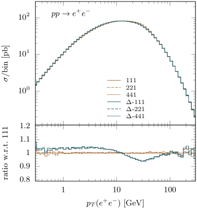
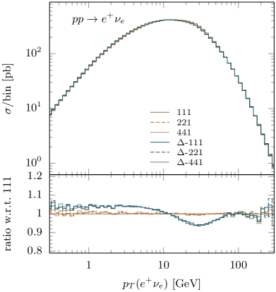
Figure 2: Transverse momentum of the $e^{+}e^{-}$ pair (left panel) and of the $e^{+}\nu_{e}$ pair (right panel), for the process in eqs. (79) and (80), respectively. Both MC@NLO (brown histograms) and MC@NLO-$\Delta$ (blue histograms) results are shown, for three choices of folding parameters.

We now turn to considering differential distributions. We point out that, for each process, we have studied the behaviour of dozens of observables, with the largest numbers in the cases of the processes with richer final states. For the sake of this paper, in view of the limitations of space it entails, we have restricted ourselves to discussing the case of an observable which is very often used as a test case in the context of matching procedures, namely the transverse momentum of the set of particles that are present in the final state at the Born level (for the process in eq. (83) such a quantity is ill-defined; we use the $W$-hardest jet system instead, which is its infrared-safe analogue). This observable has several appealing features. For example, it constitutes a practical choice for the pull introduced in eq. (18); thus, it is very directly connected to the mechanism of the reduction of negative-weight events which is central to this work. Furthermore, by simply considering a sufficiently large domain, one can separately assess the behaviour of the matched predictions in the soft/collinear, intermediate, and hard regions. This is helpful also because the theoretical systematics due to matching (at least, in MC@NLO-type prescriptions) is mostly concentrated in the intermediate region; therefore, such an observable is essentially a worst-case scenario as far as this systematics is concerned. Indeed, for the purpose of a comparison between MC@NLO and MC@NLO-$\Delta$ predictions, we have verified that the conclusions that can be drawn by studying the transverse momentum of the Born system have a rather general validity, in that by far and large they encompass the cases of the other observables that we have considered.

Our results are displayed in figs. 2–4 for the processes in eqs. (79)–(84); the case of $t\bar{t}$ production will be dealt with later (see sect. 5.1). These figures feature two panels, each relevant to a specific process, composed of a main frame and a lower inset, and all have the same layout. In the main frame there are six histograms, three of which are relevant to MC@NLO predictions (brown lines) and the other three to MC@NLO-$\Delta$ predictions (blue lines). The three results in each set differ from each other by the choice of the folding parameters: $(n_{\xi},n_{y},n_{\varphi})=(1,1,1)$ (i.e. no folding; solid), $(n_{\xi},n_{y},n_{\varphi})=(2,2,1)$ (dashed), and $(n_{\xi},n_{y},n_{\varphi})=(4,4,1)$ (dotted). Thus, the six curves in the main frames correspond to the six results associated with each process in table 1. The lower insets of the figures show the bin-by-bin ratios of each of the histograms that appear in the main frames, over the histogram relevant to the corresponding MC@NLO result with no folding; the same plotting patterns as in the main frames are employed.

In fig. 2 we present the predictions for the $Z$- (left panel) and $W^{+}$-mediated (right panel) first-family lepton pair production of eqs. (79) and (80); not surprisingly, they look very similar to each other, and the only reason to show both of them is their prominence for both SM measurements and new-physics searches at the LHC. The MC@NLO and MC@NLO-$\Delta$ results are within $\pm 5$% of each other in the whole range considered. They coincide in absolute value at large $p_{\scriptscriptstyle T}$, in keeping with one of the defining features of the MC@NLO matching, namely that in hard regions both the shape and the normalisation must coincide, up to small shower effects, with the underlying fixed-order NLO prediction. This shows that such a feature is also exhibited by MC@NLO-$\Delta$, as is expected by construction. At small transverse momenta the MC@NLO and MC@NLO-$\Delta$ results have the same shapes, which in the case of the former matching prescription is known to coincide with that of the underlying parton-shower MC; again, this shows that this property holds for MC@NLO-$\Delta$ as well. As was anticipated, the differences between MC@NLO and MC@NLO-$\Delta$ are visible in the intermediate-$p_{\scriptscriptstyle T}$ region, and must be attributed to matching systematics; in fact, they are of the same order as those one would obtain e.g. by varying the $f_{\alpha}$ parameters that control the starting scale(s) of the parton showers; we shall give in sect. 5.1 an explicit example on this point. We finally remark that, for both of the matching prescriptions, the differences between the results obtained with different folding parameters are statistically compatible with zero, which confirms the nature of the folding as a technical tool which has no impact on physics predictions.

  

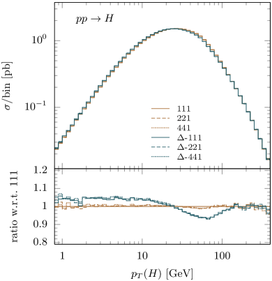
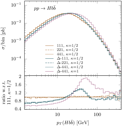
Figure 3: As in fig. 2, for the transverse momentum of the Higgs (left panel) and of the $Hb\bar{b}$ system (right panel), for the processes in eqs. (81) and (82), respectively. The latter displays an additional MC@NLO-$\Delta$ curve (red dotted); see the text for details, in particular eq. (86) for the definition of the parameter $\kappa$.

In fig. 3 we show the results for production processes that feature an SM Higgs – single-inclusive (eq. (81)) in the left panel, and in association with a $b\bar{b}$ pair (eq. (82)) in the right panel. As far as single-inclusive production is concerned, the same comments as for the lepton-pair processes of fig. 2 can be repeated verbatim. While this fact could have been expected, it is nevertheless an excellent test of the MC@NLO-$\Delta$ machinery. In fact, the production of lepton pairs is dominated by $q\bar{q}$ annihilation, that of Higgs by $gg$ fusion; as a consequence of this, the structures of the $\Delta$ factors relevant to the two cases are very different from each other.

The situation visibly changes for $Hb\bar{b}$ production, which is a process notoriously affected by very large systematics (see e.g. ref. deFlorian:2016spz ). Thus, although the qualitative pattern of the MC@NLO vs MC@NLO-$\Delta$ comparison is similar to that of the other processes considered so far, in absolute value the differences are larger, up to $\pm 30$%. We observe that the MC@NLO-$\Delta$ results are harder than the MC@NLO ones (i.e. the peak of the distribution is at larger $p_{\scriptscriptstyle T}$ values). A by-product of this fact is that the transition between the peak and the tail regimes appears to be more regular for MC@NLO-$\Delta$ than for MC@NLO – in the latter case, the histograms are flatter in the region $20~{}\,\textrm{GeV}\lesssim p_{\scriptscriptstyle T}\lesssim 70~{}\,\textrm{GeV}$. We also point out that, following ref. Wiesemann:2014ioa , $Hb\bar{b}$ production has been simulated with the parameters of eq. (88). Interestingly, in the case of MC@NLO, the choice of eq. (87) in conjunction with the reference scale of eq. (89) (i.e. a combination that had not been considered in ref. Wiesemann:2014ioa ) leads, for some observables, to a pathological behaviour – the distribution and the large fraction of negative-weight events render their cancellation a very difficult task, so that the results are always affected by dominant statistical uncertainties. It is therefore reassuring that this is not the case for MC@NLO-$\Delta$: in fig. 3 we show the result for this matching prescription (and one choice of folding parameters, the others being statistically identical to it) obtained with eq. (87) (red dotted histogram); this result is as well behaved as those obtained with eq. (88). It is clear that large matching uncertainties remain, but this appears to be characteristic of this production process at this perturbative order; if anything, the present MC@NLO-$\Delta$ systematics are smaller than their MC@NLO counterparts of ref. Wiesemann:2014ioa (see in particular fig. 5 there).

  

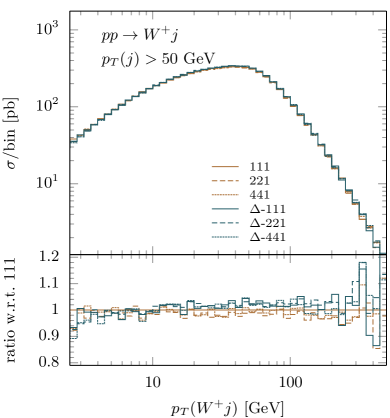
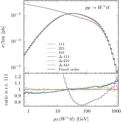
Figure 4: As in fig. 2, for the transverse momentum of the $W$-hardest jet system (left panel) and of the $W^{+}t\bar{t}$ system (right panel), for the processes in eqs. (83) and (84), respectively. In the right panel, the fixed-order result (red solid) is also shown.

We finally turn to discussing $W^{+}$ production in association with a light jet (eq. (83), left panel of fig. 4) and with a $t\bar{t}$ pair (eq. (84), right panel of fig. 4). In the case of the former process, a $p_{\scriptscriptstyle T}\geq 50~{}\,\textrm{GeV}$ cut on the $R=0.5$, anti-$k_{\scriptscriptstyle T}$ hardest jet is imposed. The MC@NLO and MC@NLO-$\Delta$ predictions for $W^{+}j$ production are rather close to each other; differences are generally smaller than $\pm 5$%. We note that the ratio plots are flatter than those relevant to the processes considered so far; this is in part because for the present observable the separation between the various regimes is not as clear-cut as in the other cases (owing to the jet-$p_{\scriptscriptstyle T}$ cut, one is more inclusive here). As far as $W^{+}t\bar{t}$ production is concerned, the differences between the MC@NLO and MC@NLO-$\Delta$ results are again quite small. However, at variance with what happens in the other processes, the MC@NLO-$\Delta$ large-$p_{\scriptscriptstyle T}$ tail is harder than the MC@NLO one. In order to investigate this point further, in fig. 4 we also display the fixed-order (FO) result (red solid histogram). This shows that the matched predictions are significantly different w.r.t. the FO one for up to very large transverse momenta; in other words, the asymptotic regime (where MC@NLO-type and FO result are expected to coincide with each other) is approached in a very slow manner; essentially, one is not yet there at the rightmost end of the range shown in fig. 4. Furthermore, the extreme steepness of the distribution at large $p_{\scriptscriptstyle T}$ implies that even small parton-shower effects might induce visible bin migrations; this is a timely reminder of the fact that, in this region, the predictions we are considering are LO-accurate in perturbation theory. We have verified that, by plotting this distribution at the level of the hard events, the MC@NLO and MC@NLO-$\Delta$ results are on top of each other, and on top of the FO one; thus, the differences between the former two predictions are indeed stemming from different shower-scale assignments.

5.1 A closer look at $t\bar{t}$ production

In this section we discuss in more details the case of $t\bar{t}$ hadroproduction (eq. (85)); this will give us the opportunity to re-consider the arguments of sect. 2 in light of a specific example. We start by considering the analogue of the observables displayed in figs. 2–4, namely the transverse momentum of the $t\bar{t}$ pair. This is shown in fig. 5, whose layout is identical to that of the figures considered so far. The conclusions are also qualitatively fairly similar to those relevant to the other processes. We note that the differences between the MC@NLO and MC@NLO-$\Delta$ predictions are larger here in the intermediate region; we anticipate (see fig. 6) that this is not the signal of a genuine discrepancy between the two prescriptions, but it rather reflects a matching uncertainty that affects both matching techniques in a similar manner. The large-$p_{\scriptscriptstyle T}$ region also exhibits some of the features relevant to $W^{+}t\bar{t}$ production that we have described in fig. 4; they are however milder here, owing to the distribution being less steep and the final-state less massive than in the previous case (thus, the asymptotic regime occurs at $p_{\scriptscriptstyle T}$ values relatively smaller than in the case of $W^{+}t\bar{t}$ production).

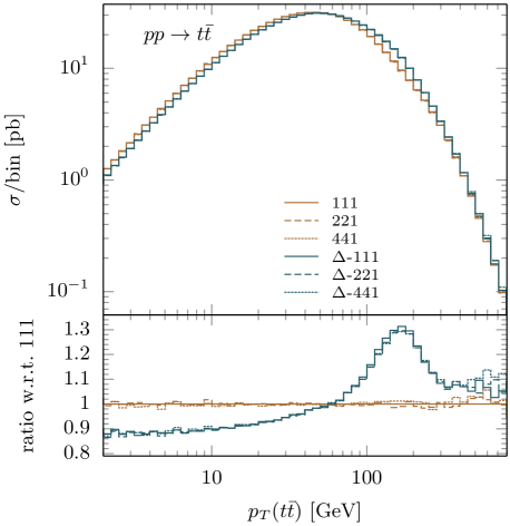
Figure 5: As in fig. 2, for the transverse momentum of the $t\bar{t}$ pair, for the process in eq. (85).

We now study how the predictions after parton showers (e.g. those in fig. 5) are related to the hard events they stem from; the reader must bear in mind that, as always in the context of MC@NLO-type matchings, the latter quantities are meaningful only in a technical, as opposed to a physical, sense. In order to do so, on top of considering the results obtained with the parameters in eq. (87), we also use what follows:

$$\kappa=1\,,\;\;\;\;\;\;\hat{f}_{1}=0.1\,,\;\;\;\;\;\;\;\hat{f}_{2}=0.55\,,$$ (91)

$$\kappa=1\,,\;\;\;\;\;\;\hat{f}_{1}=0.55\,,\;\;\;\;\;\;\hat{f}_{2}=1\,.$$ (92)

We call the settings of eqs. (87), (91), and (92) the baseline, lower, and upper choices respectively, and abbreviate these names where necessary as b, l, and u. We stress that this notation has no phenomenological implications. In other words, we do not claim that the baseline choice should be regarded as the default option when a comparison to data is performed; it is simply the choice of settings which is formally closest to the one usually adopted in MG5_aMC MC@NLO simulations. Whether it is the baseline, the lower, or the upper settings (or something else altogether) that are best for phenomenological MC@NLO-$\Delta$ applications is an open question, which is beyond the scope of the present paper.

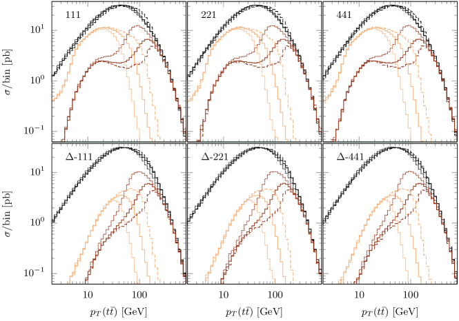
Figure 6: Transverse momentum of the $t\bar{t}$ pair, after parton showers (black histograms), and before parton showers for positive-weight (dark brown histograms) and negative-weight (light brown histograms) events; see the text for details.

In fig. 6 we consider again the transverse momentum of the $t\bar{t}$ pair. There are six panels in the figure, and all of them have the same layout. The black histograms are the MC@NLO (upper row) and MC@NLO-$\Delta$ (lower row) results; by definition, they are obtained after parton showers. The brown histograms represent results at the hard-event level, i.e. before parton showers; the dark-brown (peaking at relatively larger $p_{\scriptscriptstyle T}$’s) and light-brown (peaking at relatively smaller $p_{\scriptscriptstyle T}$’s) ones are associated with positive-weight and negative-weight events, respectively; in order to display them together, the latter are plotted by flipping their signs. Note that only ${\mathbb{H}}$ events contribute to the hard-event histograms, since for ${\mathbb{S}}$ events one has $p_{\scriptscriptstyle T}(t\bar{t})=0$, which is outside the domain of fig. 6. For each type of histogram (after parton showers and before parton showers with event weights of either sign) there are three curves; the dotted, solid, and dashed ones are obtained with the lower (eq. (91)), baseline (eq. (87)), and upper (eq. (92)) settings, respectively. It follows that the solid black histograms are the same predictions as those already shown in fig. 5 as blue curves. The three panels in each of the two rows of fig. 6 differ by the choice of the folding parameters.

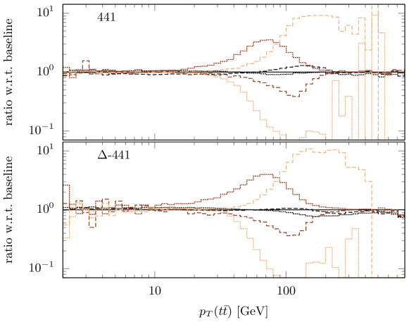
Figure 7: Ratios of the upper and lower predictions over the baseline ones, for the two rightmost panels of the two rows in fig. 6.

There are several pieces of information that can be extracted from fig. 6. We start by observing that the three panels on each row are essentially indistinguishable from one another. This is what we expect, since they differ by the choice of the folding parameters; such a choice must induce differences statistically compatible with zero for physical distributions (black histograms), and must not affect ${\mathbb{H}}$-event distributions (brown histograms) – note that the latter statement would not be true in the case of ${\mathbb{S}}$ events, as we shall document below. The choice of the $\hat{f}_{\alpha}$ parameters gives a measure of the matching systematics after parton showers; we note that such systematics (identified as the cumulative difference among the three black histograms that appear on any given panel) are very similar, but not identical, in MC@NLO and MC@NLO-$\Delta$; this confirms that, for precision studies, MC@NLO-$\Delta$ matching uncertainties are best assessed independently of the corresponding MC@NLO ones. As was anticipated, the MC@NLO and MC@NLO-$\Delta$ systematics emerging from fig. 6 are consistent with the differences between the MC@NLO and MC@NLO-$\Delta$ predictions of fig. 5 (i.e. at most a relative  $30$% effect, but typically smaller than that). At variance with the physical results, those at the hard-event level (brown histograms) exhibit a very strong dependence on the $\hat{f}_{\alpha}$ parameters (up to a relative factor of $5$ ($10$) w.r.t. the central results for the dark brown (light brown) curves): this need not be surprising, owing to their unphysical nature. However, such a large dependence offers one the possibility of a better understanding of the interplay between positive weights, negative weights, and scale assignments (whose general features have been introduced and discussed in sect. 2). In order to give a more quantitative idea of the sizes of the effects we have just discussed, we present in fig. 7 the ratios of the upper and lower predictions over the corresponding baseline ones, for the rightmost panels in the two rows of fig. 6, that correspond to the $(4,4,1)$ choice of the folding parameters – the pattern emerging from other folding-parameter choices is the same as that of fig. 7.

In order to proceed, we note preliminarily that the hard-event distributions in fig. 6 are nothing but the distribution in $p_{\scriptscriptstyle T}(t\bar{t})$ as is predicted solely by the short-distance cross section $d\sigma^{\scriptscriptstyle({\mathbb{H}})}$ (for MC@NLO, see eq. (8)) and $d\sigma^{\scriptscriptstyle(\Delta,{\mathbb{H}})}$ (for MC@NLO-$\Delta$, see eq. (23)); one simply plots the positive and negative contributions separately. This follows from the fact that by not performing parton showers one leaves the parton-level kinematical configurations unchanged. Furthermore, we remark that the value of $p_{\scriptscriptstyle T}(t\bar{t})$ is a good estimate of the stopping scale relevant to the Sudakov form factor that dominates in the construction of $\Delta$ (i.e. the smallest one); as far as the corresponding starting scale is concerned, its value will be in the range $(\kappa\hat{f}_{1}\mu_{t},\kappa\hat{f}_{2}\mu_{t})$ (see eqs. (50) and (51)), with $\mu_{t}$ predominantly of the order of the top mass; on average, the starting scale will be roughly equal to $\kappa(\hat{f}_{1}+\hat{f}_{2})\mu_{t}/2$.

As the comparison of eq. (9) with eq. (24) shows, we have:

$$d\sigma^{\scriptscriptstyle(\Delta,{\mathbb{H}})}=d\sigma^{\scriptscriptstyle({\mathbb{H}})}\Delta\equiv\big{(}d\sigma^{\scriptscriptstyle{(\rm NLO},E)}-d\sigma^{\scriptscriptstyle\rm(MC)}\big{)}\Delta\,.$$ (93)

One of the implications of what has been said about the stopping and starting scales is that $\Delta\to 0$ for small $p_{\scriptscriptstyle T}(t\bar{t})$. Thus, the cross section in this region must be much smaller in MC@NLO-$\Delta$ than in MC@NLO – this is what one sees by comparing the brown histograms in the lower row of fig. 6 with the corresponding upper-row ones, the differences being increasingly large as one moves towards $p_{\scriptscriptstyle T}(t\bar{t})=0$. This mechanism is the anticipated suppression of N.1 events in MC@NLO-$\Delta$ w.r.t. those in MC@NLO; as is expected, positive-weight events are suppressed as well, but this does not lead to a degradation of the statistical accuracy as is explained just before sect. 3.1.

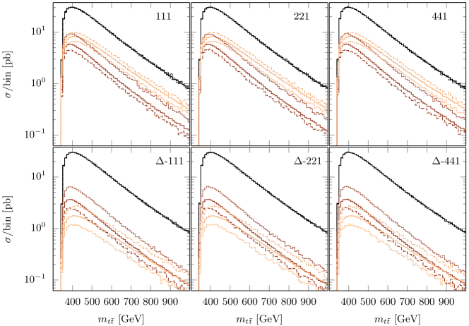
Figure 8: As in fig. 6 for the invariant mass of the $t\bar{t}$ pair. For hard events before parton shower, only ${\mathbb{H}}$ ones are shown.

The comparisons between the dotted, solid, and dashed brown histograms relevant to the same type of events (i.e. with positive or negative weights) show that the dependence on the choice of the lower, baseline, and upper settings is negligible at small $p_{\scriptscriptstyle T}(t\bar{t})$, but becomes visible at larger transverse momenta; this is a feature present in both MC@NLO and MC@NLO-$\Delta$ predictions, and can be understood as follows. The values of the $\hat{f}_{\alpha}$ parameters affect the starting scales, but not the stopping scale; accordingly, there is a corresponding dependence of the $\Delta$ factor. However, such a dependence is never particularly large, being roughly equal to the ratio of the Sudakovs that dominate in the $\Delta$ factor, computed at the different starting scales (see eq. (95)); since the latter are typically large, these Sudakovs are then of order one, and so is their ratio. Furthermore, as the stopping scale tends towards zero, the values of $\Delta$ become quite small, so that $d\sigma^{\scriptscriptstyle(\Delta,{\mathbb{H}})}$ is vanishingly small as well; this implies that the modest dependence of $\Delta$ on $\hat{f}_{\alpha}$ hardly changes the cross section (in other words, a large suppression factor is as effective as the same suppression factor multiplied by a number of order one). Things do change at larger $p_{\scriptscriptstyle T}(t\bar{t})$: here, the situation is complicated by the fact that the dependence of the short-distance cross section on $\hat{f}_{\alpha}$ is due not only to the $\Delta$ factor, but also to the function $D$ that appears in the MC counterterms (see eq. (42); note that $D=1$ for small transverse momenta). For any given $p_{\scriptscriptstyle T}(t\bar{t})$, the $\hat{f}_{\alpha}$ dependencies of these quantities result in competing effects in the case of MC@NLO-$\Delta$, while only the latter is present in MC@NLO (owing to the absence of $\Delta$ there): larger $\hat{f}_{\alpha}$ give smaller $\Delta$ (i.e. more suppression of both positive- and negative-weight events in MC@NLO-$\Delta$) and larger $D$ values (i.e. larger MC counterterms and therefore more negative-weight events in both MC@NLO-$\Delta$ and MC@NLO; see eq. (46)). Which of the two mechanisms is dominant in MC@NLO-$\Delta$ depends on the kinematical regions one is interested in. In general, given the functional form of the Sudakov form factors, and in particular the way in which they approach the value of one, as $p_{\scriptscriptstyle T}(t\bar{t})$ increases the effect of the $\Delta$ factor is subdominant w.r.t. that of the $D$ function, a fortiori in the case of MC@NLO. This appears to imply that, perhaps contrary to naive expectations, smaller $\hat{f}_{\alpha}$ are more effective in reducing negative-weight events not only in MC@NLO, but in MC@NLO-$\Delta$ as well. However, it is important to stress that, while the mechanisms described here have a general validity, their relative balance in MC@NLO-$\Delta$ is delicate, and dependent on the process. As far as $t\bar{t}$ production is concerned, we shall later document how the conclusion above can be quantified.

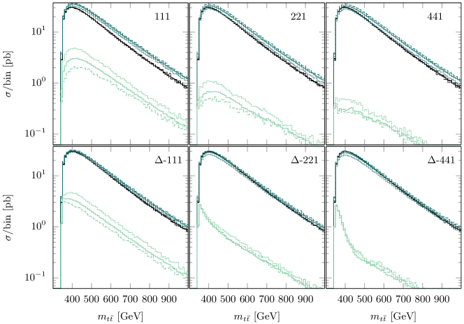
Figure 9: As in fig. 8, for ${\mathbb{S}}$ events rather than for ${\mathbb{H}}$ events.

In terms of the classification of negative-weight events given in sect. 2, we can recapitulate the discussion above by saying that the factor $\Delta$ primarily affects the number of N.1 events and, to a lesser extent, that of N.2 events. As far as the $D$ function is concerned, it mostly affects the number of N.2 events, and only marginally that of N.1 events. Thus, in MC@NLO-$\Delta$ by decreasing (increasing) the $\hat{f}_{\alpha}$ values one eliminates less (more) N.1 events, while simultaneously eliminating more (less) N.2 events. In MC@NLO, only the N.2 events are affected.

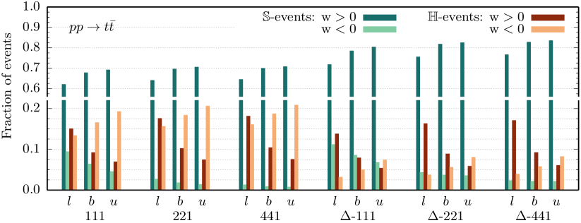
Figure 10: Fractions of positive- and negative-weight events, for both ${\mathbb{S}}$ and ${\mathbb{H}}$ events, in $t\bar{t}$ production.

Before summarising our findings, we present plots which are the analogues of those in fig. 6, but are relevant to the invariant mass of the $t\bar{t}$ pair rather than to $p_{\scriptscriptstyle T}(t\bar{t})$. The results are shown in fig. 8 and fig. 9. The layout of fig. 8 is exactly the same as that of fig. 6, namely predictions after parton shower (black histograms) and before parton shower for ${\mathbb{H}}$ events (brown histograms). In fig. 9 we display the same physical results as in fig. 8, but the distributions at the hard-event level are obtained with ${\mathbb{S}}$ events, rather than with ${\mathbb{H}}$ events – at variance with the case of the $t\bar{t}$ pair transverse momentum, ${\mathbb{S}}$-event contributions are non-trivial in the whole $m_{t\bar{t}}$ range, and are in fact the dominant ones. Positive- and negative-weight ${\mathbb{S}}$-event distributions are displayed as dark- (relatively larger cross sections) and light-green (relatively smaller cross sections) histograms, respectively. The interpretation of figs. 8 and 9 is not as easy as that of fig. 6, owing to the fact that the pair invariant mass is not a pull variable. Therefore, all of the effects that we have discussed for $p_{\scriptscriptstyle T}(t\bar{t})$ simultaneously contribute to the same $m_{t\bar{t}}$ value, and are impossible to disentangle, although for example the pattern associated with the choices of the $\hat{f}_{\alpha}$ parameters can still be seen. Furthermore, fig. 9 presents one with the direct evidence of the effects of the folding, which cannot be seen in the ${\mathbb{H}}$-event distributions of figs. 6 and 8, in particular for what concerns the reduction of N.3 events.

We conclude this section by presenting a summary of the situation of the fractions of positive- and negative-weight events in $t\bar{t}$ production, fully inclusive over all kinematical variables. In other words, we simply count the number of positive and negative weights present in the various LHE files, and divide them by the total number of events; by using the notation introduced in sect. 1, these ratios are therefore equal to $1-f$ and $f$, respectively, when ${\mathbb{S}}$ and ${\mathbb{H}}$ events are considered together. By keeping the ${\mathbb{S}}$- and ${\mathbb{H}}$-event contributions separate from each other, we obtain the results shown in fig. 10. In that figure, there are three groups of four bins for each of the three MC@NLO and MC@NLO-$\Delta$ scenarios (no folding, $221$ folding, and $441$ folding) that we have considered. Each one of such groups corresponds to a choice of the $\hat{f}_{\alpha}$ parameters, and is labelled accordingly: lower choice (l, left), baseline choice (b, center), and upper choice (u, right). Finally, the four bins in each group give the fractions of the various events w.r.t. the total number of events (i.e. the sum of the contents of the four bins is always equal to one); from left to right, positive-weight ${\mathbb{S}}$ events (dark green), negative-weight ${\mathbb{S}}$ events (light green), positive-weight ${\mathbb{H}}$ events (dark brown), and negative-weight ${\mathbb{H}}$ events (light brown). In summary, the information contained in each of the bins of fig. 10 is the phase-space integrated version of that given, at the differential level, by the brown and green histograms in figs. 6–9.

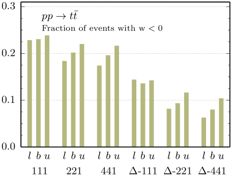
Figure 11: Fractions of negative-weight events, in $t\bar{t}$ production.

It should be noted that, by normalising all fractions to the total number of events, in both MC@NLO and MC@NLO-$\Delta$ matchings when folding is applied both of the fractions relevant to ${\mathbb{H}}$ events increase (w.r.t. the case of no folding), while either the negative- or the positive-weight fraction of ${\mathbb{S}}$ events decreases; in non-pathological situations, it is the former that decreases and the latter that increases. We point out that this is just a by-product of the chosen normalisation, and that the short-distance cross sections have the behaviour already described in sects. 2 and 3, namely that the ${\mathbb{H}}$-event cross section is unaffected by folding, while the negative contributions to the ${\mathbb{S}}$-event one are reduced. Furthermore, when ${\mathbb{S}}$ and ${\mathbb{H}}$ events are considered together, the total fraction of negative weights always decreases with folding (see fig. 11). Figure 10 summarises what we have discussed so far. For a given choice of the $\hat{f}_{\alpha}$ and folding parameters, we see a marked decrease in the fraction of negative-weight ${\mathbb{H}}$ events, and a slight increase in that of negative-weight ${\mathbb{S}}$ events, in MC@NLO-$\Delta$ w.r.t. MC@NLO. For a given choice of the $\hat{f}_{\alpha}$ parameters, in both MC@NLO and MC@NLO-$\Delta$ by folding one visibly reduces the fraction of negative-weight ${\mathbb{S}}$ events. The overall fraction ($f$) of negative-weight events that results from the various scenarios is presented in fig. 11, which re-iterates the anticipated fact that folding is always advantageous. In conclusion, figs. 10 and 11 confirm in more details and for the specific case of $t\bar{t}$ production the message that emerges from table 1: the reduction of the relative cost is achieved by moving from MC@NLO to MC@NLO-$\Delta$, and by increasing the amount of folding. The relative cost also depends on the parameters that control the assignments of the starting scales; although the latter might thus be used to further reduce it, this operation must follow their tuning to data, and within the uncertainties associated with such a tuning.

6 Conclusions

In this paper we have introduced a new NLO-accurate matching prescription, that we have called MC@NLO-$\Delta$, by starting from the MC@NLO cross section and by augmenting it with further elements of parton-shower MC origin, with the ultimate goal of reducing the number of negative-weight events that are present in MC@NLO simulations. We have achieved a practical implementation of the MC@NLO-$\Delta$ matching, by including it in the MadGraph5_aMC@NLO framework in conjunction with the Pythia8 MC. We have also taken this opportunity to implement in MadGraph5_aMC@NLO the folding Nason:2007vt technique, which induces a (further) reduction of negative-weight events in both MC@NLO-$\Delta$ and MC@NLO. Finally, we have shown how the MC@NLO-$\Delta$ matching naturally results in the inclusion, in the hard events eventually to be processed by the MC, of as many shower scales as there are oriented colour connections; thus, there are one (in the case of quarks) or two (in the case of gluons) scales per external strongly-interacting particle. This is expected to give a better modelling w.r.t. the one which is currently in use, based on a single shower scale per event.

We have presented a systematic comparison of the MC@NLO and MC@NLO-$\Delta$ predictions for seven processes in hadronic collisions at $\sqrt{S}=13$ TeV, which constitute a typical set of applications of NLO-matched computations to LHC physics. The conclusion emerging from such a comparison is that the combination of the MC@NLO-$\Delta$ matching and of folding leads to a significant reduction of the number of negative weights that affect MC@NLO simulations.

Although the physical results we have presented are based on the Pythia8 MC, as is the case for MC@NLO the MC@NLO-$\Delta$ matching has a general validity, and can be applied to any parton shower MC. However, one must bear in mind that technically the structure of the implementation in MadGraph5_aMC@NLO of the MC@NLO-$\Delta$ matching is more involved w.r.t. that of MC@NLO, since at variance with the latter it requires calling MC modules also during the event-generation phase. Therefore, in order to replicate this structure in the case of another MC, the latter should be flexible enough to allow for this (which should be the case for any modern C$++$-based MC). Alternatively, the relevant modules should be extracted from the MC and included in the MadGraph5_aMC@NLO (or, in general, the matrix-element provider) code. For completeness, we mention that such modules must include the capability, for any given kinematical configuration, of computing the Sudakov form factors that enter the definition of $\Delta$, of returning the stopping shower scales, and of deciding whether the given configuration is in an MC dead zone or not.

Reducing the number of negative-weight events is always advantageous from a statistical viewpoint; an elementary quantitative analysis is given in sect. 1. However, as far as the associated financial costs are concerned, one must take into account that such a reduction is generally accompanied by an increase of the cost per event (see eq. (7)); importantly, this is limited to the event-generation phase, and it stems from the longer running times necessary to achieve the reduction. This is the case for both the folding (which affects both MC@NLO and MC@NLO-$\Delta$; the increase in running time is limited from above by the product of the folding parameters, and is usually about 75% of that number), and the $\Delta$ prescription itself (in our Pythia8 implementation, the running time increases by a factor 2–3 for all of the processes we have considered, with the largest increases affecting the simplest ones). Neither of these aspects should be important in the balance costs/benefits in the context of full experimental simulations, while they deserve consideration for purely-theoretical studies. Both are liable to be improved by streamlining their underlying software structures.

We conclude by observing that while MC@NLO-$\Delta$ originates from the MC@NLO prescription, it is a novel matching technique, whose implications must not be assumed to be identical to those of MC@NLO. In particular, we have shown that the physics predictions for several hadroproduction processes that originate from MC@NLO and MC@NLO-$\Delta$ are fairly similar to each other. However, exactly because they are not identical, the parameter settings that are optimal for phenomenology studies are most likely not the same in the two cases; this fact has to be taken into account when comparing MC@NLO-$\Delta$ results with experimental data. From the theoretical viewpoint, on top of the differences inherent to the matching, those stemming from the novel multi-scale structure of hard-event files will also deserve careful consideration.

Appendix A The Sudakovs in Pythia8

In this appendix we report on some of the technical details relevant to the pre-tabulation of the Pythia8 Sudakov form factors, which we have introduced in sect. 4.

We start by observing that the Sudakovs are defined by means of eq. (36); in view of this, it is convenient to construct the look-up tables for $\Delta_{a}^{(*)}$ rather than for $\Delta_{a}$, owing to the simpler functional dependence of the former w.r.t. that of the latter. The direct dependence of $\Delta_{a}^{(*)}$ on the colour line $\ell$ amounts to knowing whether the beginning and the end of $\ell$ are in the initial or in the final state. There are therefore four possible cases, namely initial-initial, initial-final, final-initial, and final-final, that we shorten as II, IF, FI, and FF, and call types; the first (second) letter identifies the beginning (end) of the colour line. We also have:

$${\mathbb{M}}=\{m_{a},m_{dip}\}\,,$$ (94)

where $m_{a}$ is the mass of particle $a$ according to the internal MC settings, and $m_{dip}$ is the generalised invariant mass of the pair colour-connected by $\ell$, defined as the (square root of the) r.h.s. of eq. (49). In practice, the dependence of Sudakovs on $m_{a}$ is essentially negligible w.r.t. the other dependencies; therefore, in our simulations we have set the value of $m_{a}$ to a fixed value, equal to the Pythia8 default for particle $a$. We also exploit the fact that:

$$\Delta_{a}^{(*)}\left(q^{2};Q^{2},\ell,{\mathbb{M}}\right)=\frac{\Delta_{a}^{(*)}\left(q^{2};Q_{\max}^{2},\ell,{\mathbb{M}}\right)}{\Delta_{a}^{(*)}\left(Q^{2};Q_{\max}^{2},\ell,{\mathbb{M}}\right)}\,.$$ (95)

In other words, thanks to eq. (95) we can obtain the functional dependence of the Sudakov on both $q^{2}$ and $Q^{2}$ in terms of a single parameter, provided that the value of $Q_{\max}^{2}$ is sufficiently large. We thus arrive at what follows:

• For each Sudakov type (II, IF, FI, FF) and particle identity ($u$, $d$, $\ldots t$, $g$ – Sudakovs for antiquarks are the same as for quarks) we set up a look-up table. There are therefore 28 tables in total.

• Each entry of a given table is the value of the corresponding $\Delta_{a}^{(*)}$ factor computed at pre-selected values of $\sqrt{q^{2}}$ and $m_{dip}$, called nodal points. In other words, a look-up table is a set of numbers associated with a two-dimensional grid, defined by the nodal points in the two-dimensional space spanned by $\sqrt{q^{2}}$ and $m_{dip}$.

The nodal points for both the $\sqrt{q^{2}}$ and $m_{dip}$ variables are chosen by means of the same functional form, namely:

$$\log_{10}\left(\frac{r(j)}{1~{}{\rm GeV}}\right)=r_{0}\left(\left(\frac{j}{j_{\max}}\right)^{b}-a\right),\;\;\;\;\;\;\;\;1\leq j\leq j_{\max}\,,$$ (96)

with $r_{0}$ and $a$ such that:

$$r(1)=r_{\min}\,,\;\;\;\;\;\;\;\;\;\;r(j_{\max})=r_{\max}\,.$$ (97)

In eqs. (96) and (97) the parameters $j_{\max}$, $b$, $r_{\min}$, and $r_{\max}$ are fixed; they must be chosen so as to optimise the distributions of the nodal points. For the simulations presented in this paper we have used the following settings:

$$b=1\,,\;\;\;\;\;\;\;\;r_{\min}=1~{}{\rm GeV}\,,\;\;\;\;\;\;\;\;r_{\max}=7~{}{\rm TeV}\,,$$ (98)

for both the $\sqrt{q^{2}}$ and $m_{dip}$ variables, and

$$j_{\max}=100~{}~{}{\rm for}~{}~{}\sqrt{q^{2}}\,,\;\;\;\;\;\;\;\;j_{\max}=50~{}~{}{\rm for}~{}~{}m_{dip}\,.$$ (99)

Equation (96) is such that there is a higher density of nodal points towards the lower end of the range, $r_{\min}$; this takes into account the fact that Sudakovs vary faster for small values of $q^{2}$ and $m_{dip}$. In order to increase (decrease) such a density one must choose larger (smaller) values of $b$ (in any case, it is best to have $b={\cal O}(1)$).

We have constructed a program (gridsudgen.f), and included it in the MG5_aMC package, that loops over the Sudakov types and particle identities; for each of these, it calls the Pythia8 module (which we briefly describe below) that computes the Sudakov for all possible pairs of nodal points. These nodal values are then written in a new program (sudakov.f) that includes interpolating instructions as well (in turn, these exploit the dfint routine of the CERN libraries, that performs a double linear interpolation). The interpolation is protected in the case of inputs which are outside of the grid of nodal points. In particular: a) if $m_{dip}$ is smaller than its minimal value or larger than its maximal value, an error is returned and the run is stopped; b) if $q^{2}$ is larger than its maximal value $Q_{\max}^{2}$, the Sudakov is set equal to one; c) if $q^{2}$ is smaller than its minimal value $q_{\min}^{2}$, the Sudakov is set either equal to zero if $q^{2}<(0.5~{}\,\textrm{GeV})^{2}$ (with $0.5$ GeV taken to be the typical low-energy MC cutoff), or equal to the value resulting from a linear interpolation between zero and the value assumed by the Sudakov at $q^{2}=q_{\min}^{2}$, if $(0.5~{}\,\textrm{GeV})^{2}\leq q^{2}<q_{\min}^{2}$. Lest the interpolating dfint routine actually extrapolates, we also set (see eq. (97)) $q_{\min}^{2}=r_{\min}^{2}$ and $Q_{\max}^{2}=r_{\max}^{2}$. Finally, sudakov.f is automatically linked to MG5_aMC when creating the executable relevant to the phase-space integration and the unweighting of events.

The user of MG5_aMC can create his/her own Sudakov pre-tabulation by running gridsudgen.f prior to any proper MG5_aMC runs. For convenience, we shall include in the package a template of sudakov.f, that should be appropriate for all applications to LHC physics (this relies on the numerical values on the r.h.s.’s of eqs. (98) and (99)).

We conclude this appendix by returning to the problem of the actual computation of the Sudakov values that constitute the entries of the pre-tabulated grids. Any such entry is equal to $\Delta_{a}^{(*)}\left(q^{2};Q_{\max}^{2},\ell,{\mathbb{M}}\right)$ (see eq. (95)); in turn, at given particle identity ($a$), Sudakov type (that fixes $\ell$), and nodal points (that fix $q^{2}$ and ${\mathbb{M}}$), this is set equal to ${\cal P}$, the no-emission probability as is computed directly by Pythia8 with the specified conditions (note that this implies that, in the case of a gluon, only one colour line, $\ell$, is considered). To this end a new Pythia8 module, called pythia_get_no_emission_prob, has been included in the code, whose return value is ${\cal P}$ and that serves as a wrapper to call lower-lying (and mostly pre-existing) Pythia8 modules.

There are two crucial aspects in the computation of ${\cal P}$ that must be stressed. We comment on each of them in turn.

Firstly, ${\cal P}$ is obtained by employing trial showering Lonnblad:2001iq ; Lonnblad:2012hz . In such a procedure, the parton shower, as is implemented in the event generator, is directly used to sample the no-emission probability, in the following way. Given the two values of the shower variable, $Q_{\max}^{2}$ and $q^{2}$, a shower is generated, at the end of which one sets:

$${\cal P}_{\rm trial} = 0\;\;\;\Longleftrightarrow\;\;\;{\rm an~{}emission~{}with~{}}q^{2}<t<Q_{\max}^{2}{\rm~{}did~{}occur}\,,$$ (100)

$${\cal P}_{\rm trial} = 1\;\;\;\Longleftrightarrow\;\;\;{\rm an~{}emission~{}with~{}}q^{2}<t<Q_{\max}^{2}{\rm~{}did~{}not~{}occur}\,.$$ (101)

The procedure is repeated $N$ times, by only changing the random numbers inherent to the showering. Note that the procedure is unitary: the number of showers that result in ${\cal P}_{\rm trial}=0$, plus the number of those leading to ${\cal P}_{\rm trial}=1$, is equal to $N$. One then defines:

$${\cal P}=\frac{1}{N}\sum_{i=1}^{N}{\cal P}_{{\rm trial},i}\,,$$ (102)

with $i$ labelling the trial showers.

Secondly, usually the no-emission probability associated with showers is not equal to $\Delta_{a}^{(*)}$ if $a$ is in the initial state. For this to happen, the evolution needs to be done forwards rather than backwards, as is typically the case in order not to lose efficiency given the constraint imposed by the value of the Bjorken $x$. Since such a constraint is irrelevant for the sake of pre-tabulation, a forward initial-state shower has been implemented, so that indeed $\Delta_{a}^{(*)}={\cal P}$ regardless of whether $a$ is in the initial or final state.

The use of forward evolution for both initial and final-state showers is convenient for pre-tabulation, but poses a technical problem. Consider the fact that any such shower is driven, among many other things, by the form of the $z$ integral in eq. (40). For reasons that will soon become clear, we re-write that integral with a more generic notation for the integration range. In the case of (anti)quark and gluon it reads, respectively, as follows:

$$S_{q} = \int^{z^{+}}_{z^{-}}dz\Big{[}\hat{P}_{qq}(z)+\hat{P}_{gq}(z)\Big{]}\,,$$ (103)

$$S_{g} = \int^{z^{+}}_{z^{-}}dz\Big{[}\hat{P}_{gg}(z)+\sum_{f}\big{(}\hat{P}_{q_{f}g}(z)+\hat{P}_{\bar{q}_{f}g}(z)\big{)}\Big{]}\,,$$ (104)

with $z^{\pm}$ defined by phase-space and momentum-conservation constraints specific to the given Sudakov type (roughly speaking, one has $z^{+}=1-\epsilon=1-\sqrt{t}/Q+{\cal O}(t/Q^{2})$). As a matter of fact, in the case of the standard backwards initial-state showers $z^{-}$ is not relevant, because the lower bound of the integration range of the integrals playing the roles of $S_{q}$ and $S_{g}$ in backward evolution is actually equal to the Bjorken $x$. Thus, for initial-state showers the definition of $z^{-}$ is simply not implemented in Pythia8. Conversely, by evolving forwards a value $z^{-}>0$ is necessary, in order to prevent the integrals of eqs. (103) and (104) from diverging owing to the $z\to 0$ soft-gluon singularity of $\hat{P}_{gq}(z)$ and $\hat{P}_{gg}(z)$. There are at least three different ways to address this issue, which we now enumerate.

1. As has been advocated in eq. (40) and in the accompanying text, set $z^{+}=1-\epsilon$ and $z^{-}=\epsilon$, by analogy with the final-state case, and because of symmetry considerations driven by the behaviour of the Altarelli-Parisi kernels under a $z\to 1-z$ transformation. By explicit computation we obtain:

   $$\frac{1}{2}\int^{1-\epsilon}_{\epsilon}dz\Big{[}\hat{P}_{qq}(z)+\hat{P}_{gq}(z)\Big{]}=-2C_{\scriptscriptstyle F}\log\epsilon-\frac{3}{2}\,C_{\scriptscriptstyle F}+{\cal O}(\epsilon)\,,\phantom{aaa}$$ (105)

   $$\frac{1}{2}\int^{1-\epsilon}_{\epsilon}dz\Big{[}\hat{P}_{gg}(z)+\sum_{f}\big{(}\hat{P}_{q_{f}g}(z)+\hat{P}_{\bar{q}_{f}g}(z)\big{)}\Big{]}=-2C_{\scriptscriptstyle A}\log\epsilon-\beta_{0}+{\cal O}(\epsilon)\,,\phantom{aaaaaa}$$ (106)

   where $\beta_{0}$ is the first coefficient of the QCD $\beta$ function, and the prefactor $1/2=1/N_{a}$ takes eq. (41) into account.

2. Set $z^{+}=1-\epsilon$ and $z^{-}=1/2$. This is another way to exploit the $z\to 1-z$ properties of the kernels, which allows one to map the $z=0$ soft singularity onto the $z=1$ one, with equivalent physical meaning. Then:

   $$\int^{1-\epsilon}_{1/2}dz\Big{[}\hat{P}_{qq}(z)+\hat{P}_{gq}(z)\Big{]}=-2C_{\scriptscriptstyle F}\log\epsilon-\frac{3}{2}\,C_{\scriptscriptstyle F}+{\cal O}(\epsilon)\,,\phantom{aaa}$$ (107)

   $$\int^{1-\epsilon}_{1/2}dz\Big{[}\hat{P}_{gg}(z)+\sum_{f}\big{(}\hat{P}_{q_{f}g}(z)+\hat{P}_{\bar{q}_{f}g}(z)\big{)}\Big{]}=-2C_{\scriptscriptstyle A}\log\epsilon-\beta_{0}+{\cal O}(\epsilon)\,.\phantom{aaaaaa}$$ (108)

   Note that the $1/2$ prefactor that appears in eqs. (105) and (106) must not be used here, owing to the reduced integration range.

3. Set $z^{+}=1-\epsilon$ and $z^{-}=0$, and damp the $z=0$ soft singularity by means of the formal replacements $\hat{P}_{ij}(z)\to z\hat{P}_{ij}(z)$. We obtain:

   $$\int^{1-\epsilon}_{0}dzz\,\Big{[}\hat{P}_{qq}(z)+\hat{P}_{gq}(z)\Big{]}=-2C_{\scriptscriptstyle F}\log\epsilon-\frac{3}{2}\,C_{\scriptscriptstyle F}+{\cal O}(\epsilon)\,,\phantom{aaa}$$ (109)

   $$\int^{1-\epsilon}_{0}dzz\,\Big{[}\hat{P}_{gg}(z)+\sum_{f}\big{(}\hat{P}_{q_{f}g}(z)+\hat{P}_{\bar{q}_{f}g}(z)\big{)}\Big{]}=-2C_{\scriptscriptstyle A}\log\epsilon-\beta_{0}+{\cal O}(\epsilon)\,.\phantom{aaaaaa}$$ (110)

   Note that the multiplication by $z$ of the kernels effectively de-symmetrises the integrands, such that a symmetry factor equal to $1/2$ must not be employed.

As the r.h.s.’s of eqs. (105)–(110) show, these strategies are equivalent at the leading and subleading terms in $\epsilon$, and differ only by terms of ${\cal O}(\epsilon)$. We have implemented all of them, and indeed have verified that the differences among their predictions are very small (note that $\epsilon$ is typically a small parameter). Heuristically, we have observed that strategy #3 leads to results which on average are the closest to those of the standard backwards shower, and we have therefore adopted it for our pre-tabulation.

We conclude this appendix by remarking that the use of trial showers, being binary in nature (see eqs. (100) and (101)) might lead to a relatively coarse result for ${\cal P}$ defined as in eq. (102). In order to alleviate this problem, we have employed $N=10^{4}$ in our pre-tabulation. However, even that level of averaging may not be sufficiently smooth to be considered continuous for our purposes. In view of this, we also make use of the shower-enhancement mechanism described in ref. Lonnblad:2012hz . This stems from multiplying the splitting kernels by a factor $C$; such an artificial enhancement has to be compensated at the level of no-emission probability – eq. (100) becomes:

$${\cal P}_{\rm trial}=\left(1-\frac{1}{C}\right)^{n}\;\;\;\Longleftrightarrow\;\;\;n\geq 1~{}{\rm emissions~{}did~{}occur~{}in~{}the~{}}(q^{2},Q_{\max}^{2}){\rm~{}range}\,,$$ (111)

while eq. (101) is unchanged. One can then still employ eq. (102). The fine-graining of the enhanced trial-shower procedure is particularly important for values of $q^{2}$ that would result in a high emission rate, i.e. in the soft/collinear regions, since there the Sudakov is a fastly-varying function. To this end, we have observed that $C\geq 3$ is sufficient for the applications we have considered in this paper.

References

- (1) S. Frixione and B. R. Webber, Matching NLO QCD computations and parton shower simulations, JHEP 06 (2002) 029, [hep-ph/0204244].
- (2) P. Nason, A New method for combining NLO QCD with shower Monte Carlo algorithms, JHEP 0411 (2004) 040, [hep-ph/0409146].
- (3) S. Hoeche, F. Krauss, M. Schonherr and F. Siegert, A critical appraisal of NLO+PS matching methods, JHEP 1209 (2012) 049, [1111.1220].
- (4) S. Platzer and S. Gieseke, Dipole Showers and Automated NLO Matching in Herwig++, Eur. Phys. J. C72 (2012) 2187, [1109.6256].
- (5) Z. Nagy and D. E. Soper, Matching parton showers to NLO computations, JHEP 0510 (2005) 024, [hep-ph/0503053].
- (6) C. W. Bauer and M. D. Schwartz, Event Generation from Effective Field Theory, Phys.Rev. D76 (2007) 074004, [hep-ph/0607296].
- (7) Z. Nagy and D. E. Soper, Parton showers with quantum interference, JHEP 0709 (2007) 114, [0706.0017].
- (8) W. T. Giele, D. A. Kosower and P. Z. Skands, A simple shower and matching algorithm, Phys.Rev. D78 (2008) 014026, [0707.3652].
- (9) C. W. Bauer, F. J. Tackmann and J. Thaler, GenEvA. I. A New framework for event generation, JHEP 0812 (2008) 010, [0801.4026].
- (10) S. Jadach, W. Placzek, S. Sapeta, A. Siodmok and M. Skrzypek, Matching NLO QCD with parton shower in Monte Carlo scheme - the KrkNLO method, JHEP 10 (2015) 052, [1503.06849].
- (11) C. Oleari and L. Reina, W +- b production in POWHEG, JHEP 08 (2011) 061, [1105.4488].
- (12) P. Nason, MINT: A Computer program for adaptive Monte Carlo integration and generation of unweighted distributions, 0709.2085.
- (13) S. Alioli, P. Nason, C. Oleari and E. Re, A general framework for implementing NLO calculations in shower Monte Carlo programs: the POWHEG BOX, JHEP 06 (2010) 043, [1002.2581].
- (14) S. Frixione, Z. Kunszt and A. Signer, Three jet cross-sections to next-to-leading order, Nucl.Phys. B467 (1996) 399–442, [hep-ph/9512328].
- (15) S. Frixione, A General approach to jet cross-sections in QCD, Nucl.Phys. B507 (1997) 295–314, [hep-ph/9706545].
- (16) R. Frederix, S. Frixione, F. Maltoni and T. Stelzer, Automation of next-to-leading order computations in QCD: The FKS subtraction, JHEP 0910 (2009) 003, [0908.4272].
- (17) J. Alwall, R. Frederix, S. Frixione, V. Hirschi, F. Maltoni, O. Mattelaer et al., The automated computation of tree-level and next-to-leading order differential cross sections, and their matching to parton shower simulations, JHEP 07 (2014) 079, [1405.0301].
- (18) R. Frederix, S. Frixione, V. Hirschi, D. Pagani, H. S. Shao and M. Zaro, The automation of next-to-leading order electroweak calculations, JHEP 07 (2018) 185, [1804.10017].
- (19) S. Hoeche, F. Krauss, M. Schonherr and F. Siegert, QCD matrix elements + parton showers: The NLO case, JHEP 04 (2013) 027, [1207.5030].
- (20) T. Sjostrand, S. Mrenna and P. Z. Skands, A Brief Introduction to PYTHIA 8.1, Comput.Phys.Commun. 178 (2008) 852–867, [0710.3820].
- (21) D. Amati, A. Bassetto, M. Ciafaloni, G. Marchesini and G. Veneziano, A Treatment of Hard Processes Sensitive to the Infrared Structure of QCD, Nucl. Phys. B173 (1980) 429–455.
- (22) S. Catani, B. R. Webber and G. Marchesini, QCD coherent branching and semiinclusive processes at large x, Nucl. Phys. B349 (1991) 635–654.
- (23) K. Odagiri, Color connection structure of supersymmetric QCD (2 2) processes, JHEP 10 (1998) 006, [hep-ph/9806531].
- (24) J. Alwall, A. Ballestrero, P. Bartalini, S. Belov, E. Boos et al., A Standard format for Les Houches event files, Comput.Phys.Commun. 176 (2007) 300–304, [hep-ph/0609017].
- (25) J. Butterworth, A. Arbey, L. Basso, S. Belov, A. Bharucha et al., The Tools and Monte Carlo working group Summary Report, 1003.1643.
- (26) R. D. Ball et al., Parton distributions with LHC data, Nucl. Phys. B867 (2013) 244–289, [1207.1303].
- (27) M. Cacciari, G. P. Salam and G. Soyez, FastJet User Manual, Eur.Phys.J. C72 (2012) 1896, [1111.6097].
- (28) M. Cacciari, G. P. Salam and G. Soyez, The Anti-k(t) jet clustering algorithm, JHEP 04 (2008) 063, [0802.1189].
- (29) M. Wiesemann, R. Frederix, S. Frixione, V. Hirschi, F. Maltoni and P. Torrielli, Higgs production in association with bottom quarks, JHEP 02 (2015) 132, [1409.5301].
- (30) LHC Higgs Cross Section Working Group collaboration, D. de Florian et al., Handbook of lhc higgs cross sections: 4. deciphering the nature of the higgs sector, 1610.07922.
- (31) L. Lonnblad, Correcting the color dipole cascade model with fixed order matrix elements, JHEP 05 (2002) 046, [hep-ph/0112284].
- (32) L. Lönnblad, Fooling Around with the Sudakov Veto Algorithm, Eur. Phys. J. C73 (2013) 2350, [1211.7204].
- (33) T. Sjostrand, A Model for Initial State Parton Showers, Phys. Lett. 157B (1985) 321–325.
- (34) T. D. Gottschalk, BACKWARDS EVOLVED INITIAL STATE PARTON SHOWERS, Nucl. Phys. B277 (1986) 700–738.
- (35) Z. Nagy and D. E. Soper, Evolution of parton showers and parton distribution functions, 2002.04125.