The MadNIS Reloaded

February 27, 2024

Abstract

In pursuit of precise and fast theory predictions for the LHC, we present an implementation of the MadNIS method in the MadGraph event generator. A series of improvements in MadNIS further enhance its efficiency and speed. We validate this implementation for realistic partonic processes and find significant gains from using modern machine learning in event generators.

 

Contents

1. 1 Introduction
2. 2 Improving MadNIS
   1. 2.1 ML implementation
   2. 2.2 Multi-channel loss
   3. 2.3 Vegas initialization
   4. 2.4 Training strategies
3. 3 Implementation and benchmarks
   1. 3.1 Reference processes
   2. 3.2 Benchmarking MadNIS features
   3. 3.3 Learning from channel weights
   4. 3.4 Scaling with jet multiplicity
4. 4 Outlook
5. A Hyperparameters
6. B Channel-weight kinematics

 

1 Introduction

One of the defining aspects of the precision-LHC program is that we compare vast amounts of scattering data with first-principle predictions. These predictions come from multi-purpose LHC event generators, for instance Pythia8 [1], MG5aMC [2], or Sherpa [3]. They start from a fundamental Lagrangian and rely on perturbative quantum field theory to provide the key part of a comprehensive simulation and inference chain. LHC simulations, including event generation, are a challenging numerical task, so we expect improvements from modern machine learning [4, 5]. These improvements cover precision and speed, which can at least in part be interchanged, on track to meet the challenges by the upcoming HL-LHC program.

Following the modular structure of event generators, we will use modern neural networks to speed up expensive scattering amplitude evaluations [6, 7, 8, 9, 10, 11, 12]. Given these amplitudes, we need to improve the phase-space integration and sampling [13, 14, 15, 16, 17, 18, 19, 20, 21, 22]. Here, precise generative networks are extremely useful. Their advantage in the LHC context is that they cover interpretable physics phase spaces, for example scattering events [23, 24, 25, 26, 27, 28, 29], parton showers [30, 31, 32, 33, 34, 35, 36, 37], and detector simulations [38, 39, 40, 41, 42, 43, 44, 45, 46, 47, 48, 49, 50, 51, 52, 53, 54, 55, 56, 57, 58, 59, 60, 61].

Generative networks for LHC physics can be trained on first-principle simulations and are easy to ship, powerful in amplifying the training data [62, 63], and — most importantly — controlled and precise [28, 64, 65, 66, 67]. Subsequent tasks for these generative networks include event subtraction [68], event unweighting [69, 70], or super-resolution enhancement [71, 72]. Their conditional versions enable new analysis methods, like probabilistic unfolding [73, 74, 75, 76, 77, 78, 79, 80, 81, 82], inference [83, 84, 85], or anomaly detection [86, 87, 88, 89, 90, 91].

Every LHC event generator covers phase space using a combination of importance sampling and a multi-channel factorization. To improve phase-space sampling through modern machine learning, we need to tackle both of these technical ingredients together. This observation is the basis of the MadNIS approach [20]. Going beyond this proof of principle, we show in this paper how MadNIS can be implemented in an actual event generator and by how much a classic event generator setup can be improved. In Sec. 2 we describe the updated MadNIS framework, including an improved loss for the network training in Sec 2.2, a fast initialization using classic importance sampling in Sec. 2.3, and an efficient training strategy in Sec. 2.4. In Sec. 3.2 we then provide detailed performance tests for a range of reference processes, and always compared to an optimized MG5aMC setup. In Sec. 3.3, we show how the MadNIS performance gains can be understood in terms of amplitude patterns and symmetries, and in Sec. 3.4 we push our implementation to its limits. As a spoiler, we will find that for challenging LHC processes, MadNIS can improve the unweighting efficiencies by an order of magnitude, a performance metric which can be translated directly into a speed gain. This gain is orthogonal to the development of faster amplitude evaluations and hardware acceleration using highly parallelized GPU farms.

2 Improving MadNIS

Before we discuss our improved ML-implementations, we briefly review the basics of multi-channel Monte Carlo. We integrate a function $f\sim|\mathcal{M}|^{2}$ over phase space

$$I[f]=\int\mathrm{d}^{D}x\,f(x)\qquad\qquad x\in\mathbb{R}^{D}\;.$$ (1)

This integral can be decomposed introducing local channel weights $\alpha_{i}(x)$ [92, 93]

$$f(x)=\sum^{n_{c}}_{i=1}\alpha_{i}(x)\;f(x)\qquad\text{with}\quad\sum^{n_{c}}_{i=1}\alpha_{i}(x)=1\quad\text{and}\quad\alpha_{i}(x)\geq 0\;,$$ (2)

This MG5aMC decomposition is different from the original multi-channel method [94, 95], which is used by Sherpa [3], or Whizard [96], as discussed in Ref. [20]. The phase-space integral now reads

$$I[f]=\sum^{n_{c}}_{i=1}I_{i}[f]=\sum^{n_{c}}_{i=1}\int\mathrm{d}^{D}x\;\alpha_{i}(x)\,f(x)\;.$$ (3)

Next, we introduce a set of channel-dependent phase-space mappings

$$x\in\mathbb{R}^{D}\quad\xleftrightarrow[\quad\leftarrow\overline{G}_{i}(z)\quad]{G_{i}(x)\rightarrow}\quad z\in[0,1]^{D}\;,$$ (4)

which parametrize properly normalized densities

$$g_{i}(x)=\left|\frac{\partial G_{i}(x)}{\partial x}\right|\qquad\text{with}\quad\int\mathrm{d}^{D}x\,g_{i}(x)=1\;.$$ (5)

The phase-space integral now covers the $D$-dimensional unit cube and can be sampled as

$$\begin{split}I[f]&=\sum^{n_{c}}_{i=1}\int\left.\frac{\mathrm{d}^{D}z}{g_{i}(x)}\;\alpha_{i}(x)f(x)\right|_{x=\overline{G}_{i}(z)}\\ &=\sum^{n_{c}}_{i=1}\int\mathrm{d}^{D}x\;g_{i}(x)\;\frac{\alpha_{i}(x)f(x)}{g_{i}(x)}\equiv\sum^{n_{c}}_{i=1}\left\langle\frac{\alpha_{i}(x)f(x)}{g_{i}(x)}\right\rangle_{x\sim g_{i}(x)}\;.\end{split}$$ (6)

Typically, physics-inspired channels are initialized with analytic mappings and then refined by an adaptive algorithm, for instance Vegas [97, 98, 99, 100, 101]. It exploits the fact that the $I_{i}[f]$ are unchanged under the mappings $G_{i}$, but the variance

$$\begin{split}\sigma_{i}^{2}\equiv\sigma_{i}^{2}\left[\frac{\alpha_{i}f}{g_{i}}\right]=\left\langle\left(\frac{\alpha_{i}(x)f(x)}{g_{i}(x)}-I_{i}[f]\right)^{2}\right\rangle_{x\sim g_{i}(x)}\\ =\left\langle\frac{\alpha_{i}(x)^{2}f(x)^{2}}{g_{i}(x)^{2}}\right\rangle_{x\sim g_{i}(x)}\;-I_{i}[f]^{2}\end{split}$$ (7)

is minimized by the optimal mapping

$$g_{i}(x)\big{|}_{\text{opt}}=\frac{\alpha_{i}(x)f(x)}{I_{i}[f]}\;,$$ (8)

so the optimal form of $g_{i}(x)$ is only defined in relation to the choice of $\alpha_{i}(x)$ and, consequently, $I_{i}[f]$.

We compute the Monte Carlo estimate of each integral using a discrete set of points,

$$I_{i}[f]=\left\langle\frac{\alpha_{i}(x)f(x)}{g_{i}(x)}\right\rangle_{x\sim g_{i}(x)}\approx\frac{1}{N_{i}}\sum_{k=1}^{N_{i}}\left.\frac{\alpha_{i}(x_{k})f(x_{k})}{g_{i}(x_{k})}\right|_{x_{k}\sim g_{i}(x)}\;.$$ (9)

In analogy, the variance gives us an estimate of the uncertainty [95],

$$\Delta_{i,N_{i}}^{2}=\frac{\sigma_{i}^{2}}{N_{i}} =\frac{1}{N_{i}}\left[\left\langle\frac{\alpha_{i}(x)^{2}f(x)^{2}}{g_{i}(x)\,q_{i}(x)}\right\rangle_{x\sim q_{i}(x)}-\left\langle\frac{\alpha_{i}(x)f(x)}{q_{i}(x)}\right\rangle_{x\sim q_{i}(x)}^{2}\right]\;.$$ (10)

Here, we rely on a different sampling density $q_{i}(x)\neq g_{i}(x)$. This appears ad-hoc, but is needed to define a properly differentiable loss function during training and will improve the performance [20]. When the variance is estimated from a finite sample, a correction factor $N_{i}/(N_{i}-1)$ has to be introduced to ensure an unbiased estimator. As the complete integral $I[f]$ is the sum of statistically independent $I_{i}[f]$, its uncertainty and variance are

$$\Delta^{2}_{N} =\sum^{n_{c}}_{i=1}\Delta^{2}_{i,N_{i}}=\sum^{n_{c}}_{i=1}\frac{\sigma^{2}_{i}}{N_{i}}\qquad\text{and}\qquad\sigma_{\text{tot}}^{2}=N\Delta^{2}_{N}=\sum^{n_{c}}_{i=1}\frac{N}{N_{i}}\sigma^{2}_{i}\;.$$ (11)

2.1 ML implementation

Starting from Eq.(6), MadNIS encodes the multi-channel weight $\alpha_{i}(x)$ and the channel mappings $G_{i}(x)$ in neural networks.

Neural channel weights

First, MadNIS employs a channel-weight neural network (CWnet) to encode the local multi-channel weights defined in Eq.(2),

$$\alpha_{i}(x)\equiv\alpha_{i\xi}(x)\;,$$ (12)

where $\xi$ denotes the network parameters. The best way to implement the normalization condition from Eq.(2) in the architecture is [20]

$$\operatorname{Softmax}\alpha_{i\xi}(x)\equiv\frac{\exp\alpha_{i\xi}(x)}{\sum_{j}\exp\alpha^{\xi}_{j}(x)}\;.$$ (13)

As the channel weights vary strongly over phase space, it helps the performance to learn them as a correction to a physically motivated prior assumption. Two well-motivated and normalized priors in MG5aMC are

$$\begin{split}\alpha_{i}^{\text{MG}}(x)&=\frac{|\mathcal{M}_{i}(x)|^{2}}{\sum_{j}|\mathcal{M}_{j}(x)|^{2}}\\ \alpha_{i}^{\text{MG}}(x)&=\frac{P_{i}(x)}{\sum_{j}P_{j}(x)}\quad\text{with}\quad P_{i}(x)=\prod_{k\in\text{prop}}\frac{1}{|p_{k}(x)^{2}-m_{k}^{2}-\mathrm{i}m_{k}\Gamma_{k}|^{2}}\;.\end{split}$$ (14)

They define the single-diagram enhanced multi-channel method [92, 93]. Relative to either of them we learn a correction

$$\begin{split}\alpha_{i\xi}(x)&=\log\alpha^{\text{MG}}_{i}(x)+\Delta_{i\xi}(x)\\ \operatorname{Softmax}\alpha_{i\xi}(x)&=\frac{\alpha^{\text{MG}}_{i}(x)\;\exp\Delta_{i\xi}(x)}{\sum_{j}[\alpha^{\text{MG}}_{j}(x)\;\exp\Delta^{\xi}_{j}(x)]}\;.\end{split}$$ (15)

We initialize the network parameters $\xi_{0}$ such that $\Delta_{i\xi}(x)=0$.

Neural importance sampling

Second, we combine analytic channel mappings and a normalizing flow for a mapping from a latent space $z$ to the phase space $x$,

$$x\in\mathbb{R}^{D}\xleftrightarrow[\hskip 31.2982pt]{\text{analytic}}y\in[0,1]^{D}\xleftrightarrow[\hskip 31.2982pt]{\text{INN}}z\in[0,1]^{D}\;.$$ (16)

This chain replaces Vegas with an invertible neural network (INN) [102], an incarnation of a normalizing flow equally fast in both directions. This INN is used for latent space refinement, where the INN links two unit hypercubes $[0,1]^{D}$. MadNIS improves the physics-inspired phase-space mappings by training an INN as part of

$$z=G_{i\theta}(x)\qquad\text{or}\qquad x=\overline{G}_{i\theta}(z)\;,$$ (17)

with the network weights $\theta$. Similar to the multi-channel weights, we use physics knowledge to simplify the task of the normalizing flow and improve its efficiency.

A crucial condition for using a normalizing flow for phase-space integration is its equally fast evaluation in both directions [20]. The building blocks of the best-suited flows are coupling layers. The INN task in Eq.(16) can, in principle, be realized with any invertible coupling layer and an additional sigmoid layer. Coupling layers [103, 104, 102] split the input $y$ into two parts, $y=(y^{A},y^{B})$, and define the forward and inverse passes as

$$\begin{pmatrix}z^{A}_{r}\\ z^{B}_{s}\end{pmatrix}=\begin{pmatrix}y^{A}_{r}\\ C(y^{B}_{s};u_{s\theta}(y^{A}))\end{pmatrix}\qquad\Leftrightarrow\qquad\begin{pmatrix}y^{A}_{r}\\ y^{B}_{s}\end{pmatrix}=\begin{pmatrix}z^{A}_{r}\\ C^{-1}(z^{B}_{s};u_{s\theta}(z^{A}))\end{pmatrix}\;,$$ (18)

The component-wise coupling transform $C$ acts on the learned function $u_{\theta}$, is invertible and has a tractable Jacobian. The Jacobian of the full mapping is

$$g(y)=\prod_{s}\frac{\partial C(y^{B}_{s};u_{s\theta}(y^{A}))}{\partial y^{B}_{s}}\;.$$ (19)

For a stable numerical performance we use rational-quadratic spline (RQS) blocks [105], where each bin is a monotonically-increasing rational-quadratic (RQ) function. They provide superior expressivity and are naturally defined on a compact interval $[a,b]$. We split the unit interval $[0,1]$ in $K$ bins with $K+1$ boundaries or knots $(y_{s}^{(k)},z_{s}^{(k)})$ $(k=0,\dots,K)$, with fixed endpoints $(0,0)$ and $(1,1)$. The $K$ widths $w_{s}$ and heights $h_{s}$ of the bins and the $K+1$ derivatives $d_{s}$ at the boundaries are constructed from the output of the network,

$$u_{s\theta}(x^{A})=(\Theta^{w}_{s},\Theta^{h}_{s},\Theta^{d}_{s})\;.$$ (20)

They are normalized as

$$\begin{split}w_{s}&=\operatorname{Softmax}\Theta_{s}^{w}\\ h_{s}&=\operatorname{Softmax}\Theta_{s}^{h}\\ d_{s}&=\frac{\operatorname{Softplus}\Theta_{s}^{d}}{\log 2}\equiv\frac{\log\left(1+\exp\Theta_{s}^{d}\right)}{\log 2}\;.\end{split}$$ (21)

In contrast to the original Ref. [105], we add learnable derivatives at the boundaries to increase expressivity, and introduce the normalization of $d_{s}$ such that $\Theta_{s}^{d}=0$ is associated with a unit derivative $d_{s}=1$. The $w$, $h$ and $d$ are then used to construct the RQ function $C$ and its derivative [105].

In Eq.(18) we see that the coupling layer describes each dimension $z_{s}^{B}$ using a learned function of all $y^{A}=z^{A}$. This way, it cannot describe correlations between different directions $z^{B}_{s}$. To encode correlations between all dimensions, we stack multiple coupling layers and permute the elements between them. The permutation changes which components are combined within $y^{A}$ and $y^{B}$. We use a deterministic set of permutations based on a logarithmic decomposition of the integral dimension [16, 20], which ensures that any element is conditioned on any other element at least once. The number of coupling blocks then scales with $\log D$.

2.2 Multi-channel loss

After encoding channel weights and importance sampling as neural networks,

$$\alpha_{i}(x)\equiv\alpha_{i\xi}(x)\qquad\text{and}\qquad g_{i}(x)\equiv g_{i\theta}(x)\;,$$ (22)

the integral in Eq.(6) is estimated as

$$I[f]=\sum^{n_{c}}_{i=1}\left\langle\frac{\alpha_{i\xi}(x)f(x)}{g_{i\theta}(x)}\right\rangle_{x\sim g_{i\theta}(x)}\;.$$ (23)

The common optimization task for both networks is given by Eq.(8). The relative contribution per sub-integral changes when we train the two networks, ruling out the use of any $f$-divergence [106] when optimizing the channel weights $\alpha_{i\xi}(x)$.

As the optimization is performed on batches with size $b\ll N$, we use a loss function that does not scale with $b$ and is independent of the number of sampled points. Moreover, the sampling density in the loss function $x\sim q_{i}(x)$ cannot coincide with the learned mapping [20]. We can directly minimize the variance as the loss function

$$\begin{split}\mathcal{L}_{\text{variance}}&=\sum^{n_{c}}_{i=1}\frac{N}{N_{i}}\sigma^{2}_{i}\\ &=\sum^{n_{c}}_{i=1}\frac{N}{N_{i}}\left(\left\langle\frac{\alpha_{i\xi}(x)^{2}f(x)^{2}}{g_{i\theta}(x)\,q_{i}(x)}\right\rangle_{x\sim q_{i}(x)}-\left\langle\frac{\alpha_{i\xi}(x)f(x)}{q_{i}(x)}\right\rangle_{x\sim q_{i}(x)}^{2}\right)\;.\end{split}$$ (24)

In practice, $q_{i}(x)\simeq g_{i\theta}(x)$ allows us to compute the loss as precisely as possible and stabilizes the combined online [107] and buffered training [20].

A critical hyperparameter in the variance loss is the distribution of sample points, $N_{i}$, during training and integral evaluation. Its optimal choice depends on the $\sigma^{2}_{i}$, and with that on $\alpha_{i}$ and $g_{i}$. While the latter are only known numerically, the optimal choice of $N_{i}$ can be computed by minimizing the loss with respect to $N_{i}$, given $N=\sum_{i}N_{i}$ [108, 95]

$$N_{i}=N\frac{\sigma_{i}}{\sum_{j}\sigma_{j}}\qquad\quad\Leftrightarrow\qquad\quad\frac{N}{N_{i}}=\frac{\sum_{j}\sigma_{j}}{\sigma_{i}}\;.$$ (25)

This known result from stratified sampling defines the improved MadNIS loss

$$\begin{split}\mathcal{L}_{\textsc{MadNIS}}&=\sum_{i=1}^{n_{c}}\left(\sum_{j=1}^{n_{c}}\sigma_{j}\right)\sigma_{i}=\left[\sum_{i=1}^{n_{c}}\sigma_{i}\right]^{2}\\ &=\left[\sum_{i=1}^{n_{c}}\left(\left\langle\frac{\alpha_{i\xi}(x)^{2}f(x)^{2}}{g_{i\theta}(x)\,q_{i}(x)}\right\rangle_{x\sim q_{i}(x)}-\left\langle\frac{\alpha_{i\xi}(x)f(x)}{q_{i}(x)}\right\rangle_{x\sim q_{i}(x)}^{2}\right)^{1/2}\right]^{2}\;.\end{split}$$ (26)

The physics information used to construct a set of integration channels is usually extracted from Feynman diagrams. MG5aMC automatically groups Feynman diagrams or channels, which are linked by permutations of the final-state particles. Because of the complications through the parton densities it does not consider permutations in the initial state. Following the MG5aMC approach, symmetry-related MadNIS channels share the same phase space mapping, but the channel-weight network has separate outputs for each channel. The $\sigma_{i}$ in the loss can be defined for individual channels or for channel groups. For processes with many channels we find that using sets of channels stabilizes the training, so we resort to this assignment as our default.

2.3 Vegas initialization

Vegas [97, 98, 99] is the classic algorithm for importance sampling to compute high-dimensional integrals. For approximately factorizing integrands Vegas is extremely efficient and converges much faster than factorized neural importance sampling, so we use use a Vegas pre-training to initialize our normalizing flow.

The standard Vegas implementation integrates the unit cube, $z_{s}\in[0,1]$ and relies on an assumed factorization of the phase space dimensions, made explicit for the phase space mapping and the corresponding sampling distribution in the second step of Eq.(16)

$$g(y)=\prod_{s=1}^{D}g(y_{s})\;.$$ (27)

In analogy to Eq.(4) it encodes sampling distributions $g$ for each dimension by dividing the unit interval into $K$ bins of equal probability but different widths $w_{k}$ with $\sum_{k}w_{k}=1$. In each interval,

$$y\in[W_{k-1},W_{k}]\qquad\text{with}\qquad W_{k}=\sum_{m=1}^{k}w_{m}\;,$$ (28)

Vegas samples uniformly,

$$g(y)=\frac{1}{Kw_{k}}\qquad\text{for}\qquad y\in[W_{k-1},W_{k}]\;,$$ (29)

such that each bin integrates to $1/K$, and their sum from Eq.(5) to

$$\int_{0}^{1}\mathrm{d}y\;g(y)=\sum^{K}_{k=1}w_{k}\;\frac{1}{Kw_{k}}=1\;.$$ (30)

In one dimension, the integrated mapping $G(x)$ from Eq.(4) is a piece-wise linear function, or linear spline,

$$G(y)=(k-1)\;\frac{1}{K}+\frac{y-W_{k-1}}{Kw_{k}}\qquad\text{for}\qquad y\in[W_{k-1},W_{k}]\;.$$ (31)

The Vegas algorithm iteratively adapts the bin widths $w_{k}$ such that the distribution $g(y)$ matches the integrand. We illustrate $g$ and $G$ with $K=20$ bins for a Gaussian mixture model in the upper panels of Fig. 1.

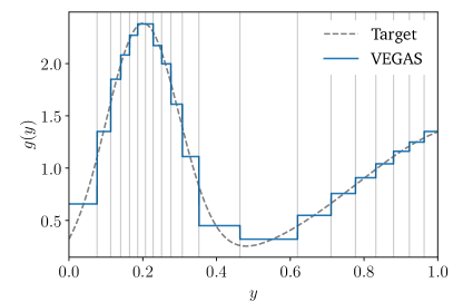
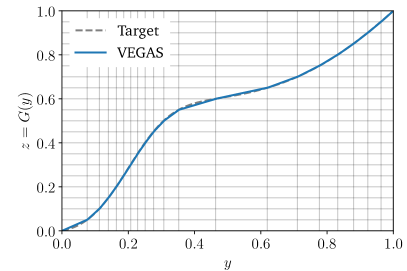
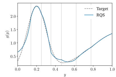
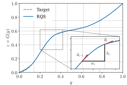
Figure 1: Top: learned Vegas density $g(x)$ with 20 bins (left) and its transformation $G(x)$ (right). Bottom: the RQS density $g(x)$ after embedding the Vegas grid and performing bin reduction to 7 bins (left). The right plot shows the corresponding mapping $G(x)$ including a zoom-in box illustrating the definition of the widths $w_{i}$, heights $h_{i}$ of the bins and the derivatives $d_{i}$ on the bin edges.

If we want to use Vegas to pre-train an INN-mapping of two unit cubes, we need to relate the Vegas grid to the RQ splines introduced in Sec. 2.1. Following Eq.(21), we need to extract the bin widths $w$, the bin heights $h$, and the derivatives on the bin edges $d$ from a Vegas grid. The width in $y$ are the same as the Vegas bin sizes, the heights are equal for all bins, and the derivatives can be estimated as the ratio of the bin heights and widths,

widths: $$\qquad w_{k} \qquad\text{for}\quad k=1,\dots,K$$

heights: $$\qquad h_{k} =\frac{1}{K} \qquad\text{for}\quad k=1,\dots,K$$

endpoints: $$\qquad d_{0} =\frac{h_{1}}{w_{1}}=\frac{1}{Kw_{1}}\qquad d_{K}=\frac{h_{K}}{w_{K}}=\frac{1}{Kw_{K}}$$

internal points: $$\qquad d_{k} =\frac{h_{k+1}+h_{k}}{w_{k+1}+w_{k}}=\frac{2}{K(w_{k+1}+w_{k})} \qquad\text{for}\quad k=1,\dots,K-1\;.$$ (32)

Because of the higher expressivity of the RQ splines, they need much fewer bins than Vegas. For instance, all bins in Vegas have equal probability, meaning that more bins than necessary are used in regions of high probability but with little change in the derivative of the transformation. We therefore reduce the number of bins by repeatedly merging adjacent bins until the desired number of target bins is reached:

1. Calculate the absolute difference between the slopes of adjacent bins,

   $$\Delta_{k}=\left|\frac{w_{k}}{h_{k}}-\frac{w_{k+1}}{h_{k+1}}\right|\;.$$ (33)

2. Choose the lowest $\Delta_{k}$, i.e. the two bins $k$ and $k+1$ with the most similar average slope. We introduce an additional cutoff, to prevent very large bins, unless all smaller bins are already merged.

3. Reduce the number of bins by one

   $$\begin{split}w&\leftarrow(w_{1},\ldots,w_{k-1},w_{k}+w_{k+1},w_{k+2},\ldots,w_{K})\;,\\ h&\leftarrow(h_{1},\ldots,h_{k-1},h_{k}+h_{k+1},h_{k+2},\ldots,h_{K})\;,\\ d&\leftarrow(d_{0},\ldots,d_{k-1},d_{k+1},\ldots,d_{K})\;,\\ K&\leftarrow K-1\;.\end{split}$$ (34)

The lower panels of Fig. 1 show $g$ and $G$ for the RQ spline after applying the bin reduction algorithm to reduce the number of bins to $K=7$. We show $w$, $h$ and $d$ for one bin.

As shown in Eq.(18), a RQS spline block includes a trainable sub-network. It encodes the bin widths $w$, heights $h$ and derivatives $d$. By inverting the normalization from Eq.(21), setting the weight matrix of the final sub-network layer to zero and assigning our results for $\Theta^{w}$, $\Theta^{h}$ and $\Theta^{d}$ to the bias vector, we can initialize the spline block to behave like the Vegas grid. This has to be done for the final two coupling blocks (in the sampling direction), one for each half of the dimensions.

2.4 Training strategies

Online & buffered training

MadNIS supports two training modes [20]. First, in the online training mode generated events are immediately used to update the network weights. Their integrands, channel weights, and Jacobians are stored for later use in the second, buffered training mode. For that, only the weight update is performed. Online training is typically more stable, especially in the early stages, while buffered training is much faster in cases where the integrand is computationally expensive. We alternate between online and buffered training and keep the buffer at a fixed size, so the oldest sample points are replaced through online training. The impact of the buffering is given by $R_{@}$, the ratio of the number of weight updates from online training to all weight updates. For expensive integrands, $R_{@}$ determines the speed gain relative to online training only. For the results shown in Sec. 3 we use a buffer size of 1000 batches and start with online training until the buffer is filled. We then train alternately on the full buffer and online, where we aim to replace either a quarter or half of the buffer, corresponding to gain factors $R_{@}=5$ and $R_{@}=3$.

Learning and correcting the channel weights changes the normalization for each channel. Since this normalization is a function of all channel weights, the complete set has to be stored as part of the buffered training. Storing $\mathcal{O}(1M)$ phase space points for a process with $\mathcal{O}(1k)$ channels requires several gigabytes, so this becomes prohibitive. On the other hand, we typically find that for a given sampling only a few channels contribute significantly. Instead of storing all weights we then store the indices and weights $(i,\alpha_{i})$ of the $m<n_{c}$ channels with the largest weights. The channel that was used to generate the sample always has to be included in this list, even if it is not among the $m$ largest weights. To optimize the network on such a buffered sample, we set the other $\alpha_{i}$ to zero and adjust the normalization accordingly. Because this approximation is only used during buffered training epochs, but not during online training, integration or sampling, it does not introduce a bias.

Stratified training & channel dropping

The variance of a channel scales with its cross section, and even if different channels contribute similarly to the total cross section, their variances can still be very imbalanced. The variance loss will be dominated by channels with a large variance, leading to large and noisy training gradients if the number of points in these channels is not sufficiently large. We improve our training by adjusting the number of points per channel and allow for channels to be dropped altogether.

Because the variance of the channels changes during the training of the channel weights and during the training of the importance sampling, we track running means of the channel variances and use them to adjust the number of points per channel during online training. To ensure a stable training we first distribute a fraction $r$ of points evenly among channels. The remaining part of the sample is distributed according to the channel variances, following the stratified sampling defined in Eq.(25). This means $r$ interpolates between uniform sampling ($r=1$) and stratified sampling ($r=0$). Note that in the presence of phase space cuts we cannot be sure that there will be points with non-vanishing weights in a given channel. For the results shown in Sec. 3 we ensure a stable estimate of the channel variance by first training with uniform $N_{i}$ for 1000 batches and then compute the variance with a running mean over the last 1000 batches.

We also go a step further and drop channels with a very small contribution to the cross section. For this, we track the running mean over the $I_{i}$ per channel and allow for channels to be dropped after every training epoch. We define a fraction of the total cross section, typically $10^{-3}\times I$, which can be neglected by dropping the corresponding channels. Next we sort all channels by $I_{i}$ and drop channels, starting from the smallest contributions, until this fraction is reached. If we drop a channel we also remove its contribution to the buffered sample and adjust the normalization of the channel weights. This way no training time is invested into dropped channels and the result remains unbiased.

3 Implementation and benchmarks

We call MG5aMC from MadNIS to compute the matrix element and parton densities, the initial phase space mapping, and the initial channel weights used in Eq.(15). For each event the inputs to this MG5aMC call are a vector of random numbers $r_{s}$ with $s=1\dots D$ and the index $i$ of the channel used to sample the event. The MG5aMC output is the concatenation of all 4-momenta $p$, the event weight $w$, and the set of channel weights $\alpha_{j}^{\text{MG}}$ with $j=1\dots n_{c}$. All MadNIS hyperparameters used for our benchmark study are given in the Appendix, Tab. 2. Currently, our interface is not fully optimized and is still a speed bottleneck. Furthermore, our setup does not support multiple partonic processes yet. Hence, we will not show run time comparisons in this work and will use processes with a fixed partonic initial state.

3.1 Reference processes

To benchmark the MadNIS performance we choose a set of realistic and challenging hard processes,

Triple-W $${\mathrm{u}}{\mathrm{\bar{d}}} \to{\mathrm{W^{+}}}{\mathrm{W^{+}}}{\mathrm{W^{-}}}\quad$$

VBS $${\mathrm{u}}{\mathrm{c}} \to{\mathrm{W^{+}}}{\mathrm{W^{+}}}\;{\mathrm{d}}{\mathrm{s}}\quad$$

W+jets $${\mathrm{g}}{\mathrm{g}} \to{\mathrm{W^{+}}}{\mathrm{d}}\bar{{\mathrm{u}}}\qquad {\mathrm{g}}{\mathrm{g}} \to{\mathrm{W^{+}}}{\mathrm{d}}\bar{{\mathrm{u}}}{\mathrm{g}}\qquad {\mathrm{g}}{\mathrm{g}} \to{\mathrm{W^{+}}}{\mathrm{d}}\bar{{\mathrm{u}}}{\mathrm{g}}{\mathrm{g}}$$

$${\mathrm{t}}{\mathrm{\bar{t}}} {\mathrm{g}}{\mathrm{g}} \to{\mathrm{t}}{\mathrm{\bar{t}}}+{\mathrm{g}}\qquad {\mathrm{g}}{\mathrm{g}} \to{\mathrm{t}}{\mathrm{\bar{t}}}+{\mathrm{g}}{\mathrm{g}}\qquad {\mathrm{g}}{\mathrm{g}} \to{\mathrm{t}}{\mathrm{\bar{t}}}+{\mathrm{g}}{\mathrm{g}}{\mathrm{g}}\;,$$+jets (35)

The produced heavy particles are assumed to be stable. The motivation for VBS and Triple-W production is that they are key to understand electroweak symmetry breaking, and that their large number of gauge-related Feynman diagrams will challenge our framework with potentially large interference. Next, we choose W+jets and ${\mathrm{t}}{\mathrm{\bar{t}}}$+jets production to study the scaling with additional jets. In Tab. 1 we show the number of Feynman diagrams and the number of MG5aMC channels for all processes. For instance, MG5aMC does not construct a separate channel for four-point vertices, so the number of channels is smaller than the number of diagrams. Channels which only differ by a permutation of the final-state momenta are combined into groups, further reducing the numbers of mappings. Finally, we show the number of channels that remain active after a MadNIS training, as discussed in Sec. 3.3.

Process		# diagrams	# channels	# channel groups	# active channels
Triple-W	${\mathrm{u}}{\mathrm{\bar{d}}}\to{\mathrm{W^{+}}}{\mathrm{W^{+}}}{\mathrm{W^{-}}}$	17	16	8	2 $\ldots$ 4
VBS	${\mathrm{u}}{\mathrm{c}}\to{\mathrm{W^{+}}}{\mathrm{W^{+}}}\;{\mathrm{d}}{\mathrm{s}}$	51	30	15	4 $\ldots$ 6
W+jets	${\mathrm{g}}{\mathrm{g}}\to{\mathrm{W^{+}}}\,{\mathrm{d}}\bar{{\mathrm{u}}}$	8	8	4	6
	${\mathrm{g}}{\mathrm{g}}\to{\mathrm{W^{+}}}\,{\mathrm{d}}\bar{{\mathrm{u}}}{\mathrm{g}}$	50	48	24	12 $\ldots$ 16
	${\mathrm{g}}{\mathrm{g}}\to{\mathrm{W^{+}}}\,{\mathrm{d}}\bar{{\mathrm{u}}}{\mathrm{g}}{\mathrm{g}}$	428	384	108	28 $\ldots$ 51
${\mathrm{t}}{\mathrm{\bar{t}}}$+jets	${\mathrm{g}}{\mathrm{g}}\to{\mathrm{t}}{\mathrm{\bar{t}}}+{\mathrm{g}}$	16	15	9	4 $\ldots$ 6
	${\mathrm{g}}{\mathrm{g}}\to{\mathrm{t}}{\mathrm{\bar{t}}}+{\mathrm{g}}{\mathrm{g}}$	123	105	35	12
	${\mathrm{g}}{\mathrm{g}}\to{\mathrm{t}}{\mathrm{\bar{t}}}+{\mathrm{g}}{\mathrm{g}}{\mathrm{g}}$	1240	945	119	60 $\ldots$ 72

Table 1: Number of Feynman diagrams, channels and channel groups after accounting for symmetries. The last column shows the number of channels that remain active after MadNIS channel dropping. Its range reflects ten independent trainings.

3.2 Benchmarking MadNIS features

To see the gain from each of the MadNIS features introduced in Sec. 2 we apply them to our reference processes one by one. Our baseline is Vegas, combined with MG5aMC channel mappings and channel weights. For a fair comparison, we also optimize Vegas to the best of knowledge and work with more iterations and larger samples than the MG5aMC default. The Vegas optimization is still significantly faster than MadNIS, but our goal is to provide a pre-trained MadNIS generator and the training time is amortized for generating large numbers of events, so the generation time is our only criterion.

We use two metrics for our comparison: (i) the relative standard deviation $\sigma/I$ minimized by stratified sampling, as is it independent from the sampling statistics and cross section; (ii) the unweighting efficiency $\epsilon$ [18], where the maximum weight is determined by bootstrapping and taking the median. For each, we use ten independent trainings and compute the means and standard deviations as an estimate of the stability of the training. We note that all obtained results, both integrated as well as differential cross-sections, agree with the default MG5aMC output and yield the correct result.

In Fig. 2 we show the results of our benchmarking for the four different processes with gauge bosons. For the more time-consuming top pair processes without any specific challenges we will provide the final improvements below.

First, we show the results from a simple setup where only the channel mappings are trained, but the channel weights are kept fixed, Sec. 2.1. Already here we see a sizeable gain over the standard method. Next, we also train the channel weights, and observe a further significant gain. For instance, the unweighting efficiency for VBS now reaches $20\%$, up from a few per-cent from the standard method and by more than a factor ten.

Next, we stick to the trainings without and with adaptive channel weights, but combine them with the Vegas-initialization from Sec. 2.3. For all processes, the gain compared to the standard Vegas method stabilizes, albeit without major improvements. This changes when we include stratified training, as introduced in Sec. 2.4. For all processes, stratified sampling with trained channel weights lead to another significant performance gain, up to a factor 15 for the VBS process.

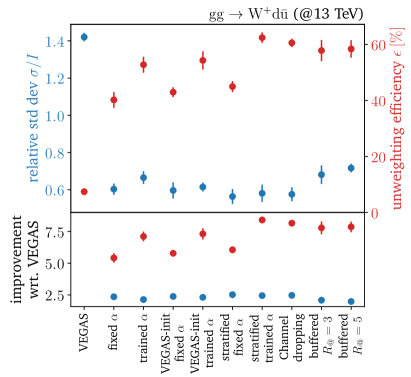
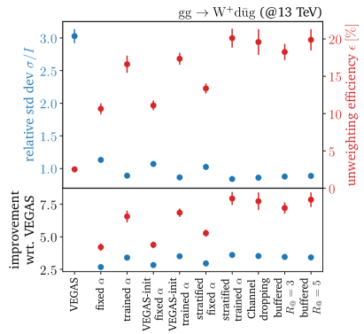
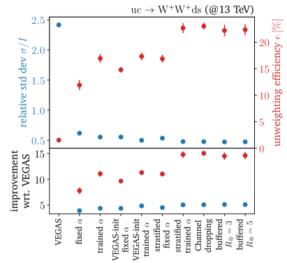
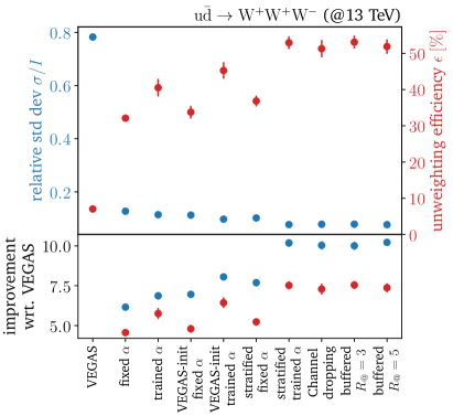
Figure 2: Relative standard deviation and unweighting efficiency for W+2jets, W+3jets, VBS and Triple-W for various combinations of MadNIS features.

Finally, we add channel dropping and buffered training, to reduce the training time. For time-wise gain factors $R_{@}=3$ and $R_{@}=5$ the improvement of the full MadNIS setup over the standard Vegas and MG5aMC integration remains stable. For processes with a large number of channels, channel dropping leads to a more stable training, while providing an equally good performance for the processes shown in Fig. 2. The fact that the performance gain for the unweighting efficiency is much larger than for the relative standard deviation reflects the sensitivity of the unweighting efficiency to the far tails of the weight distribution.

3.3 Learning from channel weights

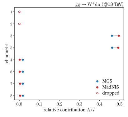
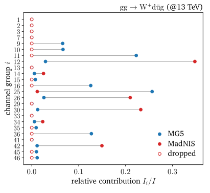
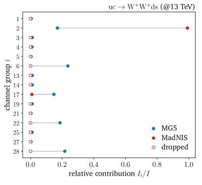
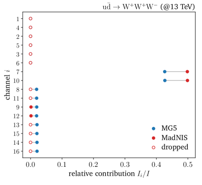
Figure 3: Relative contributions of the channels for W+2jets and Triple-W production, and for the channel groups for W+3jets and VBS. The channel weights are defined by MG5aMC, their weights are learned by MadNIS. An empty circle indicates a dropped channel.

It turns our that we can also extract information from the learned channel weights. We look at the contribution of each channel to the total cross section,

$$\frac{I_{i}}{I}=\frac{\int\mathrm{d}^{D}x\;\alpha_{i}(x)\,f(x)}{\int\mathrm{d}^{D}x\;f(x)}\;,$$ (36)

We find that MadNIS changes the contribution of channel groups coherently, so for W+3jets and Triple-W production we look at the contributions given by the sum over the channels in the group.

In Fig. 3, we show the contribution of MadNIS channels or channel groups, compared to the initial MG5aMC assignments. We mark dropped channels with empty circles, the number of remaining active channels corresponds to Tab. 1. We see that MadNIS prefers much fewer channels, illustrating the benefit of our channel dropping feature.

For VBS and Triple-W production, MadNIS adapts the channel weights in a way that the integrand is almost completely made up from a single group of symmetry-related channels. The general behaviour and the specific choice of channels is consistent between repetitions of the training. The Feynman diagrams corresponding to these channels are shown in Fig. 4. For VBS five channel groups significantly contribute to the integral in MG5aMC, all of them with a $t$-channel gluon or photon. Of those, MadNIS enhances the QCD contribution $\mathcal{O}(\alpha_{s}^{2}\alpha^{2})$ without an $s$-channel quark propagator. For Triple-W production, one channel group already dominates the integral in MG5aMC, and it is further enhanced by MadNIS. We give an example for the distribution learned by the learned channel weights as a function of phase space in Appendix B.

Figure 4: Feynman diagrams corresponding to the dominant channels after training MadNIS for VBS (left) and Triple-W production (right).

3.4 Scaling with jet multiplicity

The last challenge of modern event generation MadNIS needs to meet is large number of additional jets. We study the scaling of the MadNIS performance with the number of gluons in the final state for W+jets and ${\mathrm{t}}{\mathrm{\bar{t}}}$+jets production. Again, we use the relative standard deviation $\sigma/I$ and the unweighting efficiency $\epsilon$ as performance metrics. As for the final result in Fig. 2, we train MadNIS with all features, including buffered training with $R_{@}=5$. The results are shown in Fig. 5. While the unweighting efficiency decreases and standard deviation increases towards higher multiplicities, the gain over Vegas and MG5aMC remains roughly constant for W+jets production. For the even more challenging ${\mathrm{t}}{\mathrm{\bar{t}}}$+jets production the gain decreases for three jets, defining a remaining task for the final, public release of MadNIS.

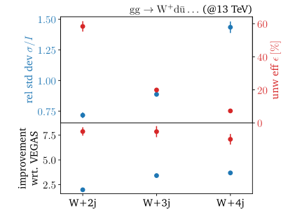
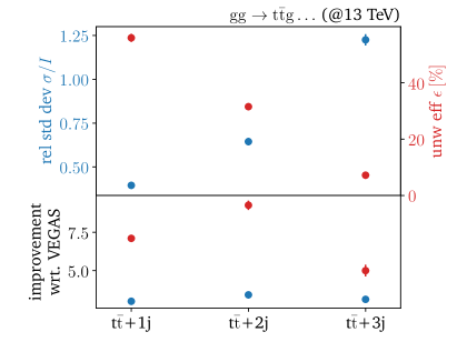
Figure 5: Relative standard deviation and unweighting efficiency for W+jets and ${\mathrm{t}}{\mathrm{\bar{t}}}$+jets with different numbers of gluons in the final state. The final MadNIS performance gain is illustrated in the lower panels, just as in Fig. 2.

4 Outlook

We have, for the first time, shown that modern machine learning leads to a significant speed gain in MG5aMC. We have improved the MadNIS method [20] and implemented it in MG5aMC, to be able to quantify the performance gain from a modern ML-treatment of phase space sampling. This implementation will allow us to use the entire MG5aMC functionality while developing an ultra-fast event generator for the HL-LHC.

Starting from a combined training of a learnable phase space mapping encoded in an INN and learnable channel weights encoded in a simple regression network, we have added a series of new feature, including an improved loss function and a fast Vegas initialization. The combined online and buffered training has been further enhanced by stratified sampling and channel dropping. The basic structure behind the phase space mapping is still a state-of-the-art INN with rational quadratic spline coupling layers, rather than more expressive diffusion networks [29], because event generation requires the mapping to be fast in both directions.

The processes we used to benchmark the MadNIS performance gain are W+2,3,4 jets, VBS, Triple-W, and ${\mathrm{t}}{\mathrm{\bar{t}}}$+1,2,3 jets. They combine large numbers of gauge-related Feynman diagrams with a large number of particles in the final state. Through MG5aMC, these key processes can easily be expanded to any other partonic production or decay process. For the electroweak reference processes we have shown the performance gain, in terms of the integration error and the unweighting efficiency, for each of our new features separately. The performance benchmark was a tuned MG5aMC implementation. It turned out that learned phase space weights, the Vegas initialization, and the stratified training each contribute to a significant performance gain. Channel dropping and buffered training stabilize the training and limit the computational cost of the network training. The MadNIS gain in the unweighting efficiency ranges between a factor 5 and a factor 15, the latter realized for the notorious VBS process.

Appendix A Hyperparameters

Parameter	Value
Optimizer	Adam [109]
Learning rate	0.001
LR schedule	Inverse decay
Final learning rate	0.0001
Batch size	$\min(200\cdot 0.8^{n_{c}},10000)$
Training length	88k batches
Permutations	Logarithmic decomposition [16]
Number of coupling blocks	$2\>\lceil\log_{2}D\rceil$
Coupling transformation	RQ splines [105]
Subnet hidden nodes	32
Subnet depth	3
CWnet parametrization	$(\log p_{T},\eta,\phi)$
CWnet hidden nodes	64
CWnet depth	3
Activation function	leaky ReLU
Max. # of buffered channel weights	75
Buffer size	1000 batches
Channel dropping cutoff	0.001
Uniform training fraction $r$	0.1
Vegas iterations	7 (7)
Vegas bins	64 (128)
Vegas samples per iteration	20k (50k)
Vegas damping $\alpha$	0.7 (0.5)

Table 2: MadNIS hyperparameters. For the Vegas parameters, the first value is used for the pre-training and the value in parentheses for the remaining runs.

Appendix B Channel-weight kinematics

To illustrate the learned channel weights we use an example with only three channels,

$${\mathrm{g}}{\mathrm{g}} \to{\mathrm{g}}{\mathrm{g}}\;.$$ (37)

This process has four Feynman diagrams, but MG5aMC only constructs mappings corresponding to the $s$, $t$ and $u$-channel Feynman diagrams. The latter two are related by an exchange of the two final-state gluons and will therefore share the same normalizing flow in MadNIS. We run a MadNIS training and use it to generate a set of weighted events. We keep the channel weights $\alpha^{\text{MG}}$ provided by MG5aMC and the $\alpha$ obtained from the CWnet. In Fig. 6, we show a stacked histogram of the $z$ component of the momentum of the first gluon, because the asymmetric structure of the $t$ and $u$ channels is best visible for this observable. Furthermore, we show the average $\alpha^{\text{MG}}$ and $\alpha$ in every bin of this histogram. In this example we see that MadNIS does not significantly change the functional form of the channel weights over phase space, but enhances the contribution of the $s$ channel, while decreasing the contributions of the $t$ and $u$ channels. This might be because MadNIS prefers channels that cover the entire phase space instead of more specialized channels for simple processes like this one.

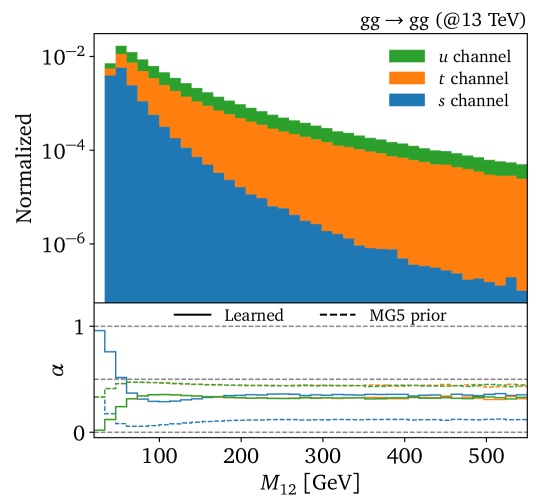
Figure 6: Stacked histogram of $z$-component of the first gluon momentum for the process ${\mathrm{g}}{\mathrm{g}}\to{\mathrm{g}}{\mathrm{g}}$ generated by MadNIS. The lower panel shows the bin-wise averages of the channels weights as obtained from MG5aMC and the learned channel weights.

References

- [1] T. Sjöstrand, S. Ask, J. R. Christiansen, R. Corke, N. Desai, P. Ilten, S. Mrenna, S. Prestel, C. O. Rasmussen, and P. Z. Skands, An introduction to PYTHIA 8.2, Comput. Phys. Commun. 191 (2015) 159, arXiv:1410.3012 [hep-ph].
- [2] J. Alwall, R. Frederix, S. Frixione, V. Hirschi, F. Maltoni, O. Mattelaer, H. S. Shao, T. Stelzer, P. Torrielli, and M. Zaro, The automated computation of tree-level and next-to-leading order differential cross sections, and their matching to parton shower simulations, JHEP 07 (2014) 079, arXiv:1405.0301 [hep-ph].
- [3] Sherpa Collaboration, Event Generation with Sherpa 2.2, SciPost Phys. 7 (2019) 3, 034, arXiv:1905.09127 [hep-ph].
- [4] S. Badger et al., Machine learning and LHC event generation, SciPost Phys. 14 (2023) 4, 079, arXiv:2203.07460 [hep-ph].
- [5] T. Plehn, A. Butter, B. Dillon, and C. Krause, Modern Machine Learning for LHC Physicists, arXiv:2211.01421 [hep-ph].
- [6] F. Bishara and M. Montull, (Machine) Learning Amplitudes for Faster Event Generation, arXiv:1912.11055 [hep-ph].
- [7] S. Badger and J. Bullock, Using neural networks for efficient evaluation of high multiplicity scattering amplitudes, JHEP 06 (2020) 114, arXiv:2002.07516 [hep-ph].
- [8] J. Aylett-Bullock, S. Badger, and R. Moodie, Optimising simulations for diphoton production at hadron colliders using amplitude neural networks, JHEP 08 (6, 2021) 066, arXiv:2106.09474 [hep-ph].
- [9] D. Maître and H. Truong, A factorisation-aware Matrix element emulator, JHEP 11 (7, 2021) 066, arXiv:2107.06625 [hep-ph].
- [10] R. Winterhalder, V. Magerya, E. Villa, S. P. Jones, M. Kerner, A. Butter, G. Heinrich, and T. Plehn, Targeting multi-loop integrals with neural networks, SciPost Phys. 12 (2022) 4, 129, arXiv:2112.09145 [hep-ph].
- [11] S. Badger, A. Butter, M. Luchmann, S. Pitz, and T. Plehn, Loop amplitudes from precision networks, SciPost Phys. Core 6 (2023) 034, arXiv:2206.14831 [hep-ph].
- [12] D. Maître and H. Truong, One-loop matrix element emulation with factorisation awareness, arXiv:2302.04005 [hep-ph].
- [13] J. Bendavid, Efficient Monte Carlo Integration Using Boosted Decision Trees and Generative Deep Neural Networks, arXiv:1707.00028 [hep-ph].
- [14] M. D. Klimek and M. Perelstein, Neural Network-Based Approach to Phase Space Integration, SciPost Phys. 9 (10, 2020) 053, arXiv:1810.11509 [hep-ph].
- [15] I.-K. Chen, M. D. Klimek, and M. Perelstein, Improved Neural Network Monte Carlo Simulation, SciPost Phys. 10 (9, 2021) 023, arXiv:2009.07819 [hep-ph].
- [16] C. Gao, J. Isaacson, and C. Krause, i-flow: High-dimensional Integration and Sampling with Normalizing Flows, Mach. Learn. Sci. Tech. 1 (1, 2020) 045023, arXiv:2001.05486 [physics.comp-ph].
- [17] E. Bothmann, T. Janßen, M. Knobbe, T. Schmale, and S. Schumann, Exploring phase space with Neural Importance Sampling, SciPost Phys. 8 (1, 2020) 069, arXiv:2001.05478 [hep-ph].
- [18] C. Gao, S. Höche, J. Isaacson, C. Krause, and H. Schulz, Event Generation with Normalizing Flows, Phys. Rev. D 101 (2020) 7, 076002, arXiv:2001.10028 [hep-ph].
- [19] K. Danziger, T. Janßen, S. Schumann, and F. Siegert, Accelerating Monte Carlo event generation – rejection sampling using neural network event-weight estimates, SciPost Phys. 12 (9, 2022) 164, arXiv:2109.11964 [hep-ph].
- [20] T. Heimel, R. Winterhalder, A. Butter, J. Isaacson, C. Krause, F. Maltoni, O. Mattelaer, and T. Plehn, MadNIS – Neural Multi-Channel Importance Sampling, SciPost Phys. 15 (2023) 141, arXiv:2212.06172 [hep-ph].
- [21] T. Janßen, D. Maître, S. Schumann, F. Siegert, and H. Truong, Unweighting multijet event generation using factorisation-aware neural networks, SciPost Phys. 15 (2023) 107, arXiv:2301.13562 [hep-ph].
- [22] E. Bothmann, T. Childers, W. Giele, F. Herren, S. Hoeche, J. Isaacsson, M. Knobbe, and R. Wang, Efficient phase-space generation for hadron collider event simulation, SciPost Phys. 15 (2023) 169, arXiv:2302.10449 [hep-ph].
- [23] S. Otten, S. Caron, W. de Swart, M. van Beekveld, L. Hendriks, C. van Leeuwen, D. Podareanu, R. Ruiz de Austri, and R. Verheyen, Event Generation and Statistical Sampling for Physics with Deep Generative Models and a Density Information Buffer, Nature Commun. 12 (2021) 1, 2985, arXiv:1901.00875 [hep-ph].
- [24] B. Hashemi, N. Amin, K. Datta, D. Olivito, and M. Pierini, LHC analysis-specific datasets with Generative Adversarial Networks, arXiv:1901.05282 [hep-ex].
- [25] R. Di Sipio, M. Faucci Giannelli, S. Ketabchi Haghighat, and S. Palazzo, DijetGAN: A Generative-Adversarial Network Approach for the Simulation of QCD Dijet Events at the LHC, JHEP 08 (2019) 110, arXiv:1903.02433 [hep-ex].
- [26] A. Butter, T. Plehn, and R. Winterhalder, How to GAN LHC Events, SciPost Phys. 7 (2019) 6, 075, arXiv:1907.03764 [hep-ph].
- [27] Y. Alanazi, N. Sato, T. Liu, W. Melnitchouk, M. P. Kuchera, E. Pritchard, M. Robertson, R. Strauss, L. Velasco, and Y. Li, Simulation of electron-proton scattering events by a Feature-Augmented and Transformed Generative Adversarial Network (FAT-GAN), arXiv:2001.11103 [hep-ph].
- [28] A. Butter, T. Heimel, S. Hummerich, T. Krebs, T. Plehn, A. Rousselot, and S. Vent, Generative networks for precision enthusiasts, SciPost Phys. 14 (2023) 4, 078, arXiv:2110.13632 [hep-ph].
- [29] A. Butter, N. Huetsch, S. P. Schweitzer, T. Plehn, P. Sorrenson, and J. Spinner, Jet Diffusion versus JetGPT – Modern Networks for the LHC, arXiv:2305.10475 [hep-ph].
- [30] L. de Oliveira, M. Paganini, and B. Nachman, Learning Particle Physics by Example: Location-Aware Generative Adversarial Networks for Physics Synthesis, Comput. Softw. Big Sci. 1 (2017) 1, 4, arXiv:1701.05927 [stat.ML].
- [31] A. Andreassen, I. Feige, C. Frye, and M. D. Schwartz, JUNIPR: a Framework for Unsupervised Machine Learning in Particle Physics, Eur. Phys. J. C 79 (2019) 2, 102, arXiv:1804.09720 [hep-ph].
- [32] E. Bothmann and L. Debbio, Reweighting a parton shower using a neural network: the final-state case, JHEP 01 (2019) 033, arXiv:1808.07802 [hep-ph].
- [33] K. Dohi, Variational Autoencoders for Jet Simulation, arXiv:2009.04842 [hep-ph].
- [34] E. Buhmann, G. Kasieczka, and J. Thaler, EPiC-GAN: Equivariant Point Cloud Generation for Particle Jets, arXiv:2301.08128 [hep-ph].
- [35] M. Leigh, D. Sengupta, G. Quétant, J. A. Raine, K. Zoch, and T. Golling, PC-JeDi: Diffusion for Particle Cloud Generation in High Energy Physics, arXiv:2303.05376 [hep-ph].
- [36] V. Mikuni, B. Nachman, and M. Pettee, Fast Point Cloud Generation with Diffusion Models in High Energy Physics, arXiv:2304.01266 [hep-ph].
- [37] E. Buhmann, C. Ewen, D. A. Faroughy, T. Golling, G. Kasieczka, M. Leigh, G. Quétant, J. A. Raine, D. Sengupta, and D. Shih, EPiC-ly Fast Particle Cloud Generation with Flow-Matching and Diffusion, arXiv:2310.00049 [hep-ph].
- [38] M. Paganini, L. de Oliveira, and B. Nachman, Accelerating Science with Generative Adversarial Networks: An Application to 3D Particle Showers in Multilayer Calorimeters, Phys. Rev. Lett. 120 (2018) 4, 042003, arXiv:1705.02355 [hep-ex].
- [39] L. de Oliveira, M. Paganini, and B. Nachman, Controlling Physical Attributes in GAN-Accelerated Simulation of Electromagnetic Calorimeters, J. Phys. Conf. Ser. 1085 (2018) 4, 042017, arXiv:1711.08813 [hep-ex].
- [40] M. Paganini, L. de Oliveira, and B. Nachman, CaloGAN : Simulating 3D high energy particle showers in multilayer electromagnetic calorimeters with generative adversarial networks, Phys. Rev. D 97 (2018) 1, 014021, arXiv:1712.10321 [hep-ex].
- [41] M. Erdmann, L. Geiger, J. Glombitza, and D. Schmidt, Generating and refining particle detector simulations using the Wasserstein distance in adversarial networks, Comput. Softw. Big Sci. 2 (2018) 1, 4, arXiv:1802.03325 [astro-ph.IM].
- [42] M. Erdmann, J. Glombitza, and T. Quast, Precise simulation of electromagnetic calorimeter showers using a Wasserstein Generative Adversarial Network, Comput. Softw. Big Sci. 3 (2019) 1, 4, arXiv:1807.01954 [physics.ins-det].
- [43] D. Belayneh et al., Calorimetry with Deep Learning: Particle Simulation and Reconstruction for Collider Physics, Eur. Phys. J. C 80 (12, 2020) 688, arXiv:1912.06794 [physics.ins-det].
- [44] E. Buhmann, S. Diefenbacher, E. Eren, F. Gaede, G. Kasieczka, A. Korol, and K. Krüger, Getting High: High Fidelity Simulation of High Granularity Calorimeters with High Speed, Comput. Softw. Big Sci. 5 (2021) 1, 13, arXiv:2005.05334 [physics.ins-det].
- [45] E. Buhmann, S. Diefenbacher, E. Eren, F. Gaede, G. Kasieczka, A. Korol, and K. Krüger, Decoding Photons: Physics in the Latent Space of a BIB-AE Generative Network, arXiv:2102.12491 [physics.ins-det].
- [46] C. Krause and D. Shih, CaloFlow: Fast and Accurate Generation of Calorimeter Showers with Normalizing Flows, arXiv:2106.05285 [physics.ins-det].
- [47] ATLAS Collaboration, AtlFast3: the next generation of fast simulation in ATLAS, Comput. Softw. Big Sci. 6 (2022) 7, arXiv:2109.02551 [hep-ex].
- [48] C. Krause and D. Shih, CaloFlow II: Even Faster and Still Accurate Generation of Calorimeter Showers with Normalizing Flows, arXiv:2110.11377 [physics.ins-det].
- [49] E. Buhmann, S. Diefenbacher, D. Hundhausen, G. Kasieczka, W. Korcari, E. Eren, F. Gaede, K. Krüger, P. McKeown, and L. Rustige, Hadrons, better, faster, stronger, Mach. Learn. Sci. Tech. 3 (2022) 2, 025014, arXiv:2112.09709 [physics.ins-det].
- [50] C. Chen, O. Cerri, T. Q. Nguyen, J. R. Vlimant, and M. Pierini, Analysis-Specific Fast Simulation at the LHC with Deep Learning, Comput. Softw. Big Sci. 5 (2021) 1, 15.
- [51] V. Mikuni and B. Nachman, Score-based generative models for calorimeter shower simulation, Phys. Rev. D 106 (2022) 9, 092009, arXiv:2206.11898 [hep-ph].
- [52] ATLAS Collaboration, Deep generative models for fast photon shower simulation in ATLAS, arXiv:2210.06204 [hep-ex].
- [53] C. Krause, I. Pang, and D. Shih, CaloFlow for CaloChallenge Dataset 1, arXiv:2210.14245 [physics.ins-det].
- [54] J. C. Cresswell, B. L. Ross, G. Loaiza-Ganem, H. Reyes-Gonzalez, M. Letizia, and A. L. Caterini, CaloMan: Fast generation of calorimeter showers with density estimation on learned manifolds, in 36th Conference on Neural Information Processing Systems. 11, 2022. arXiv:2211.15380 [hep-ph].
- [55] S. Diefenbacher, E. Eren, F. Gaede, G. Kasieczka, C. Krause, I. Shekhzadeh, and D. Shih, L2LFlows: Generating High-Fidelity 3D Calorimeter Images, arXiv:2302.11594 [physics.ins-det].
- [56] H. Hashemi, N. Hartmann, S. Sharifzadeh, J. Kahn, and T. Kuhr, Ultra-High-Resolution Detector Simulation with Intra-Event Aware GAN and Self-Supervised Relational Reasoning, arXiv:2303.08046 [physics.ins-det].
- [57] A. Xu, S. Han, X. Ju, and H. Wang, Generative Machine Learning for Detector Response Modeling with a Conditional Normalizing Flow, arXiv:2303.10148 [hep-ex].
- [58] S. Diefenbacher, E. Eren, F. Gaede, G. Kasieczka, A. Korol, K. Krüger, P. McKeown, and L. Rustige, New Angles on Fast Calorimeter Shower Simulation, arXiv:2303.18150 [physics.ins-det].
- [59] E. Buhmann, S. Diefenbacher, E. Eren, F. Gaede, G. Kasieczka, A. Korol, W. Korcari, K. Krüger, and P. McKeown, CaloClouds: Fast Geometry-Independent Highly-Granular Calorimeter Simulation, arXiv:2305.04847 [physics.ins-det].
- [60] M. R. Buckley, C. Krause, I. Pang, and D. Shih, Inductive CaloFlow, arXiv:2305.11934 [physics.ins-det].
- [61] S. Diefenbacher, V. Mikuni, and B. Nachman, Refining Fast Calorimeter Simulations with a Schrödinger Bridge, arXiv:2308.12339 [physics.ins-det].
- [62] A. Butter, S. Diefenbacher, G. Kasieczka, B. Nachman, and T. Plehn, GANplifying event samples, SciPost Phys. 10 (2021) 6, 139, arXiv:2008.06545 [hep-ph].
- [63] S. Bieringer, A. Butter, S. Diefenbacher, E. Eren, F. Gaede, D. Hundhausen, G. Kasieczka, B. Nachman, T. Plehn, and M. Trabs, Calomplification — the power of generative calorimeter models, JINST 17 (2022) 09, P09028, arXiv:2202.07352 [hep-ph].
- [64] R. Winterhalder, M. Bellagente, and B. Nachman, Latent Space Refinement for Deep Generative Models, arXiv:2106.00792 [stat.ML].
- [65] B. Nachman and R. Winterhalder, ELSA – Enhanced latent spaces for improved collider simulations, arXiv:2305.07696 [hep-ph].
- [66] M. Leigh, D. Sengupta, J. A. Raine, G. Quétant, and T. Golling, PC-Droid: Faster diffusion and improved quality for particle cloud generation, arXiv:2307.06836 [hep-ex].
- [67] R. Das, L. Favaro, T. Heimel, C. Krause, T. Plehn, and D. Shih, How to Understand Limitations of Generative Networks, arXiv:2305.16774 [hep-ph].
- [68] A. Butter, T. Plehn, and R. Winterhalder, How to GAN Event Subtraction, SciPost Phys. Core 3 (12, 2019) 009, arXiv:1912.08824 [hep-ph].
- [69] B. Stienen and R. Verheyen, Phase Space Sampling and Inference from Weighted Events with Autoregressive Flows, SciPost Phys. 10 (11, 2021) 038, arXiv:2011.13445 [hep-ph].
- [70] M. Backes, A. Butter, T. Plehn, and R. Winterhalder, How to GAN Event Unweighting, SciPost Phys. 10 (2021) 4, 089, arXiv:2012.07873 [hep-ph].
- [71] F. A. Di Bello, S. Ganguly, E. Gross, M. Kado, M. Pitt, L. Santi, and J. Shlomi, Towards a Computer Vision Particle Flow, Eur. Phys. J. C 81 (2021) 2, 107, arXiv:2003.08863 [physics.data-an].
- [72] P. Baldi, L. Blecher, A. Butter, J. Collado, J. N. Howard, F. Keilbach, T. Plehn, G. Kasieczka, and D. Whiteson, How to GAN Higher Jet Resolution, SciPost Phys. 13 (2022) 3, 064, arXiv:2012.11944 [hep-ph].
- [73] K. Datta, D. Kar, and D. Roy, Unfolding with Generative Adversarial Networks, arXiv:1806.00433 [physics.data-an].
- [74] M. Bellagente, A. Butter, G. Kasieczka, T. Plehn, and R. Winterhalder, How to GAN away Detector Effects, SciPost Phys. 8 (2020) 4, 070, arXiv:1912.00477 [hep-ph].
- [75] A. Andreassen, P. T. Komiske, E. M. Metodiev, B. Nachman, and J. Thaler, OmniFold: A Method to Simultaneously Unfold All Observables, Phys. Rev. Lett. 124 (2020) 18, 182001, arXiv:1911.09107 [hep-ph].
- [76] M. Bellagente, A. Butter, G. Kasieczka, T. Plehn, A. Rousselot, R. Winterhalder, L. Ardizzone, and U. Köthe, Invertible Networks or Partons to Detector and Back Again, SciPost Phys. 9 (2020) 074, arXiv:2006.06685 [hep-ph].
- [77] M. Backes, A. Butter, M. Dunford, and B. Malaescu, An unfolding method based on conditional Invertible Neural Networks (cINN) using iterative training, arXiv:2212.08674 [hep-ph].
- [78] M. Leigh, J. A. Raine, and T. Golling, -Flows: conditional neutrino regression, arXiv:2207.00664 [hep-ph].
- [79] J. A. Raine, M. Leigh, K. Zoch, and T. Golling, -Flows: Fast and improved neutrino reconstruction in multi-neutrino final states with conditional normalizing flows, arXiv:2307.02405 [hep-ph].
- [80] A. Shmakov, K. Greif, M. Fenton, A. Ghosh, P. Baldi, and D. Whiteson, End-To-End Latent Variational Diffusion Models for Inverse Problems in High Energy Physics, arXiv:2305.10399 [hep-ex].
- [81] J. Ackerschott, R. K. Barman, D. Gonçalves, T. Heimel, and T. Plehn, Returning CP-Observables to The Frames They Belong, arXiv:2308.00027 [hep-ph].
- [82] S. Diefenbacher, G.-H. Liu, V. Mikuni, B. Nachman, and W. Nie, Improving Generative Model-based Unfolding with Schrödinger Bridges, arXiv:2308.12351 [hep-ph].
- [83] S. Bieringer, A. Butter, T. Heimel, S. Höche, U. Köthe, T. Plehn, and S. T. Radev, Measuring QCD Splittings with Invertible Networks, SciPost Phys. 10 (2021) 6, 126, arXiv:2012.09873 [hep-ph].
- [84] A. Butter, T. Heimel, T. Martini, S. Peitzsch, and T. Plehn, Two Invertible Networks for the Matrix Element Method, SciPost Phys. 15 (2023) 094, arXiv:2210.00019 [hep-ph].
- [85] T. Heimel, N. Huetsch, R. Winterhalder, T. Plehn, and A. Butter, Precision-Machine Learning for the Matrix Element Method, arXiv:2310.07752 [hep-ph].
- [86] B. Nachman and D. Shih, Anomaly Detection with Density Estimation, Phys. Rev. D 101 (2020) 075042, arXiv:2001.04990 [hep-ph].
- [87] A. Hallin, J. Isaacson, G. Kasieczka, C. Krause, B. Nachman, T. Quadfasel, M. Schlaffer, D. Shih, and M. Sommerhalder, Classifying anomalies through outer density estimation, Phys. Rev. D 106 (9, 2022) 055006, arXiv:2109.00546 [hep-ph].
- [88] J. A. Raine, S. Klein, D. Sengupta, and T. Golling, CURTAINs for your sliding window: Constructing unobserved regions by transforming adjacent intervals, Front. Big Data 6 (2023) 899345, arXiv:2203.09470 [hep-ph].
- [89] A. Hallin, G. Kasieczka, T. Quadfasel, D. Shih, and M. Sommerhalder, Resonant anomaly detection without background sculpting, arXiv:2210.14924 [hep-ph].
- [90] T. Golling, S. Klein, R. Mastandrea, and B. Nachman, FETA: Flow-Enhanced Transportation for Anomaly Detection, arXiv:2212.11285 [hep-ph].
- [91] D. Sengupta, S. Klein, J. A. Raine, and T. Golling, CURTAINs Flows For Flows: Constructing Unobserved Regions with Maximum Likelihood Estimation, arXiv:2305.04646 [hep-ph].
- [92] F. Maltoni and T. Stelzer, MadEvent: Automatic event generation with MadGraph, JHEP 02 (2003) 027, arXiv:hep-ph/0208156.
- [93] O. Mattelaer and K. Ostrolenk, Speeding up MadGraph5_aMC@NLO, Eur. Phys. J. C 81 (2021) 5, 435, arXiv:2102.00773 [hep-ph].
- [94] R. Kleiss and R. Pittau, Weight optimization in multichannel Monte Carlo, Comput. Phys. Commun. 83 (1994) 141, arXiv:hep-ph/9405257.
- [95] S. Weinzierl, Introduction to Monte Carlo methods, arXiv:hep-ph/0006269.
- [96] W. Kilian, T. Ohl, and J. Reuter, WHIZARD: Simulating Multi-Particle Processes at LHC and ILC, Eur. Phys. J. C 71 (2011) 1742, arXiv:0708.4233 [hep-ph].
- [97] G. P. Lepage, A New Algorithm for Adaptive Multidimensional Integration, J. Comput. Phys. 27 (1978) 192.
- [98] G. P. Lepage, VEGAS: AN ADAPTIVE MULTIDIMENSIONAL INTEGRATION PROGRAM, .
- [99] G. P. Lepage, Adaptive multidimensional integration: VEGAS enhanced, J. Comput. Phys. 439 (2021) 110386, arXiv:2009.05112 [physics.comp-ph].
- [100] T. Ohl, Vegas revisited: Adaptive Monte Carlo integration beyond factorization, Comput. Phys. Commun. 120 (1999) 13, arXiv:hep-ph/9806432.
- [101] S. Brass, W. Kilian, and J. Reuter, Parallel Adaptive Monte Carlo Integration with the Event Generator WHIZARD, Eur. Phys. J. C 79 (2019) 4, 344, arXiv:1811.09711 [hep-ph].
- [102] L. Ardizzone, J. Kruse, S. Wirkert, D. Rahner, E. W. Pellegrini, R. S. Klessen, L. Maier-Hein, C. Rother, and U. Köthe, Analyzing inverse problems with invertible neural networks, International Conference on Learning Representations (8, 2018) , arXiv:1808.04730 [cs.LG].
- [103] L. Dinh, D. Krueger, and Y. Bengio, Nice: Non-linear independent components estimation, arXiv:1410.8516 [cs.LG].
- [104] L. Dinh, J. Sohl-Dickstein, and S. Bengio, Density estimation using real nvp, arXiv:1605.08803 [cs.LG].
- [105] C. Durkan, A. Bekasov, I. Murray, and G. Papamakarios, Neural spline flows, Advances in Neural Information Processing Systems 32 (6, 2019) 7511, arXiv:1906.04032 [stat.ML].
- [106] F. Nielsen and R. Nock, On the chi square and higher-order chi distances for approximating f-divergences, IEEE Signal Processing Letters 21 (Jan, 2014) 10–13, arXiv:1309.3029 [cs.IT].
- [107] A. Butter, S. Diefenbacher, G. Kasieczka, B. Nachman, T. Plehn, D. Shih, and R. Winterhalder, Ephemeral Learning - Augmenting Triggers with Online-Trained Normalizing Flows, SciPost Phys. 13 (2022) 4, 087, arXiv:2202.09375 [hep-ph].
- [108] W. H. Press and G. R. Farrar, Recursive stratified sampling for multidimensional monte carlo integration, Computers in Physics 4 (1990) 2, 190.
- [109] D. P. Kingma and J. Ba, Adam: A Method for Stochastic Optimization, arXiv:1412.6980 [cs.LG].