The use of hypermodels to understand binary neutron star collisions

Abstract

Gravitational waves from the collision of binary neutron stars provide a unique opportunity to study the behaviour of supranuclear matter, the fundamental properties of gravity, and the cosmic history of our Universe. However, given the complexity of Einstein’s Field Equations, theoretical models that enable source-property inference suffer from systematic uncertainties due to simplifying assumptions. We develop a hypermodel approach to compare and measure the uncertainty of gravitational-wave approximants. Using state-of-the-art models, we apply this new technique to the binary neutron star observations GW170817 and GW190425 and to the sub-threshold candidate GW200311_103121. Our analysis reveals subtle systematic differences (with Bayesian odds of $\sim 2$) between waveform models. A frequency-dependence study suggests that this may be due to the treatment of the tidal sector. This new technique provides a proving ground for model development and a means to identify waveform-systematics in future observing runs where detector improvements will increase the number and clarity of binary neutron star collisions we observe.

Department of Physics, Royal Holloway, University of London, TW20 0EX, United Kingdom

University of Portsmouth, Institute of Cosmology and Gravitation, Portsmouth PO1 3FX, United Kingdom

Institute for Physics and Astronomy, University of Potsdam, D-14476 Potsdam, Germany

Max Planck Institute for Gravitational Physics (Albert Einstein Institute), Am Mühlenberg 1, D-14476 Potsdam, Germany

1 Challenges in gravitational-wave modelling

The first detection of gravitational waves and electromagnetic signals originating from the same astrophysical source, the merger of two neutron stars GW170817[1], revolutionised astronomy and led to advances in numerous scientific fields, e.g., a new and independent way to measure the Hubble constant[2, 3, 4], the proof that neutron star mergers are a cosmic source of heavy elements[5, 6, 7, 8], tight constraints on alternative theories of gravity[9, 10, 11], and a measurement of the propagation speed of gravitational waves[12]. Since this breakthrough detection, the LIGO-Scientific and Virgo Collaborations have observed a second binary neutron star merger GW190425[13] and reported the sub-threshold candidate GW200311_103121[14].

Astrophysical inferences about gravitational-wave events rely on an accurate measurement of the source properties, e.g., the mass and spin of the component stars, the luminosity distance, and the tidal properties. Measuring these properties is part of the inverse problem. Typically, a Bayesian inference approach is applied, which requires $\mathcal{O}(10^{8})$ model evaluations to robustly infer the posterior distribution for the tens of parameters that describe a binary neutron star merger. Given the complexity of Einstein’s Field Equations, which govern the final stages of the coalescence, the direct computation of gravitational waveforms is a challenging task. State-of-the-art numerical-relativity simulations, in which the equations of general relativity and general-relativistic hydrodynamics are solved, require considerable resources on high-performance computing centres to model the dynamics and gravitational-signal emitted shortly before the merger of the two neutron stars. Despite their need for millions of CPU hours, these simulations allow only the study of the last 10 to 20 orbits before the collision[15, 16, 17]. On the other hand, the Advanced LIGO[18] and Virgo[19] detectors have a broadband sensitivity which enables them to measure several thousand orbits before the merger. Given these restrictions, the direct computation of gravitational-waveform models to solve the inverse problem for binary merger events is impossible.

Therefore, the analysis of gravitational-wave signals of binary neutron star systems relies on the usage of analytical and semi-analytical approximant models. These approximant models are either based on the Post-Newtonian (PN) framework[20], a perturbative approach to solve Einstein’s Field equations for small velocities and large distances, on the effective-one-body (EOB) approach[21, 22], in which the relativistic two-body problem is mapped into an effective one-body description, or simplified phenomenological models that incorporate PN knowledge and are calibrated through EOB and numerical-relativity data[23]. With these approaches, the approximant models can be evaluated in a few tens of milliseconds, enabling the source properties to be inferred in a few days.

The gravitational-wave community has made significant progress in improving these waveform approximants over the last few years. Higher tidal PN contributions have been computed[20], different tidal EOB approximants have been developed[24, 25, 26], and numerous phenomenological models have been derived[23, 27, 28]. To this extent, the reliability of waveform approximants was always checked against numerical-relativity simulations, which introduces additional challenges. First, the error assessment of general-relativistic hydrodynamics simulations is complicated due to the formation of shocks and discontinuities in the matter fields. Second, the simulations can only cover the late inspiral. Therefore, although there have been works that showed possible waveform systematic biases for future detections[29, 30, 31, 32, 33], a qualitative judgment about the accuracy of the waveform models has always been difficult.

The standard approach to account for intrinsic modelling errors is to study differences between the inferred posterior distribution for a set of approximant models. Then, these differences in the posteriors are investigated through the direct computation of a few numerical-relativity waveforms in the problematic parameter space region with the goal to understand if the differences point to a deficiency of one or more of the models. If the models hold up under investigation, the differences are ascribed to “waveform systematics”. To produce posterior distributions, which account for waveform systematics, it is usual to mix together the posterior distribution from different approximants. This process yields a posterior distribution marginalised over the uncertainty inherent in the predefined set of models. Typically[14], this is done by mixing together the equal-weighted posteriors from each model. However, an equal-weighted approach neglects information provided by the Bayesian evidence; it is instead preferable to mix posteriors according to their relative Bayesian evidence[34]. This process also provides a means to study model selection using the Bayesian odds between models. However, the previous approach[34] suffers two difficulties. First, it relies on estimation of the Bayesian evidence and uncertainty using, for example, the Nested Sampling algorithm[35]. The robustness of such a result can be difficult to guarantee in practice and, as we show in Section 5, the method developed herein can achieve more precise measurement of the odds at nearly equal computational expense compared to the evidence-weighting approach. Second, from a pragmatic point of view, it is sometimes problematic to ensure independent analyses are identical in all respects except the model approximant. This is because slight differences in, for example, the analysed data systematically impact the Bayesian evidence and can result in systematic errors which are difficult to identify.

In this work (see Section 5), we develop a new data-driven validation of gravitational-wave approximants using the idea of hypermodels: simultaneously inferring the source properties of the event by applying stochastic sampling to a predefined set of waveform models. Building on a similar grid-based approach[36], this technique can produce posterior inferences directly marginalising over the hypermodel set, capturing the intrinsic modelling uncertainty But, it also enables inferences about the predictions of individual models in the hypermodel set and the plausibility of each model relative to all other models in the set. This allows us to understand which of the existing waveform models is preferred and describes the observational data best. By varying the choice of frequency-domain data, we can show how the method can reveal in which frequency range noticeable differences between the models occur, which leads to insights about the models themselves.

2 Inferring information from gravitational-wave data

We apply our new method to study the first two confidently detected binary neutron star signals observed by the Advanced LIGO and Advanced Virgo detectors, GW170817[1] and GW190425[13], and the sub-threshold candidate GW200311_103121 recently reported in the GWTC3 catalogue[14]. We analyse the data with four cutting-edge spin-aligned waveform approximant models for binary neutron star mergers: IMRPhenomD_NRTidalv2[37, 38, 27], SEOBNRv4_ROM_NRTidalv2[39, 27], SEOBNRv4T_surrogate[26, 40], and TEOBResumS[41]. All four approximants, neglect the effects of precession (analyses of binary neutron star systems using precessing waveform models demonstrate the effect is negligible[42, 13]), but include matter-effects through the tidal parameters.

For each event, we analyse $128\text{\,}\mathrm{s}$ of data covering the event and use the on-source Power Spectral Density computed by BayesLine [43] and published with the original discovery. For GW170817 and GW200311_103121, we analyse the frequency-domain data from $23\text{\,}\mathrm{H}\mathrm{z}$ to $2048\text{\,}\mathrm{H}\mathrm{z}$, while for GW190425 we analyse data from $20\text{\,}\mathrm{H}\mathrm{z}$ to $2048\text{\,}\mathrm{H}\mathrm{z}$ (the difference in the lower bound arises from the different total mass of the systems). Unlike the original analyses, we exclude the marginalisation over the systematic error in the measured astrophysical strain due to the detector calibration. This error is sub-dominant to the systematic errors from waveform modelling,[44] and we, therefore, neglect it. We apply an astrophysically motivated[45] low spin prior, restricting the dimensional spin magnitudes of each component to be less than 0.05, where this bound is derived from observed binary neutron star systems and theoretical spin estimates at their respective moment of the merger. For other parameters, we use non-informative priors, i.e., uniform in the component masses with cuts made in the chirp mass and mass ratio and uninformative priors for all other parameters.[46] The exception to this is the analysis of GW170817, in which we fix the sky location to that of the observed electromagnetic counterpart.

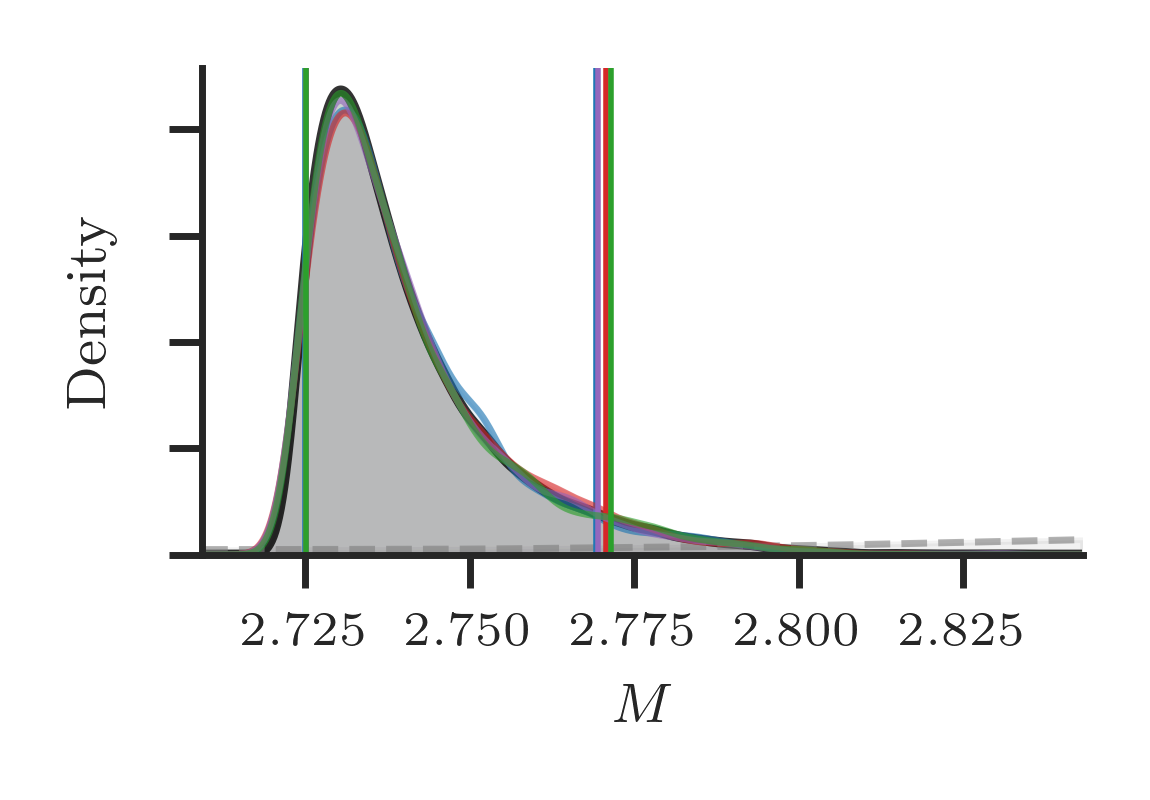
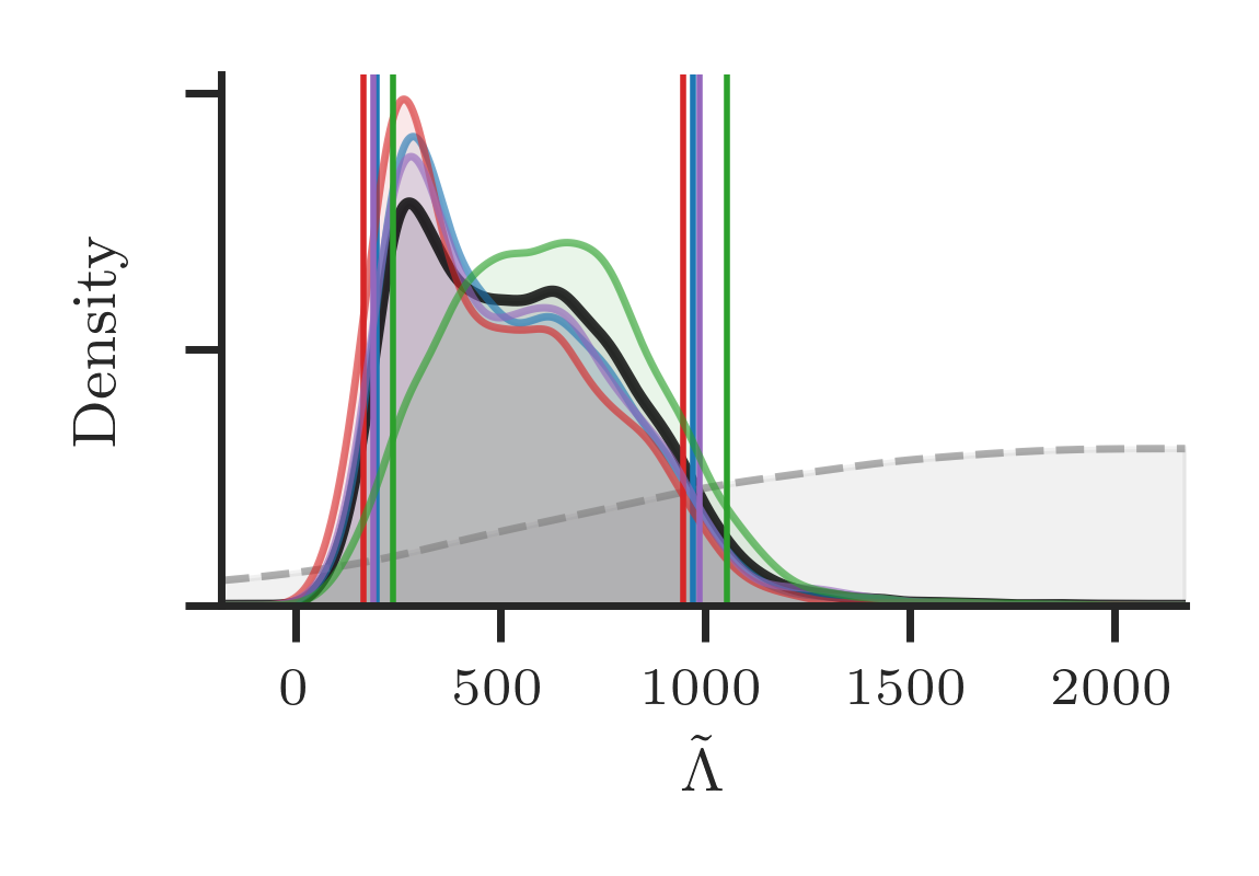
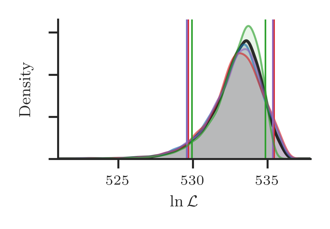
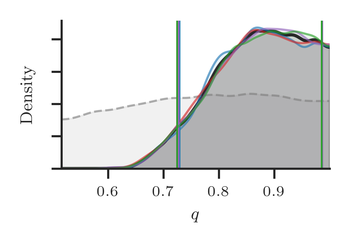
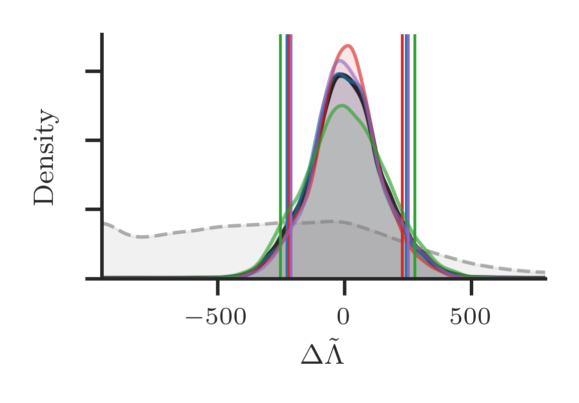
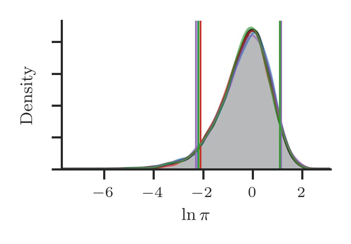
Figure 1: Posterior densities for the mass and tidal deformability of GW170817. We show the combined posteriors, marginalized over all waveform models using the hypermodel approach, and the posteriors for each individual model, extracted from the combined posterior, as well. The dashed curve provides the prior distribution estimated by drawing samples. In the right-hand column, we include the distributions of the log-likelihood and log-prior of the posterior samples.

Waveform	GW170817		GW190425		GW200311_103121		Joint
	Prob. [%]	odds	Prob. [%]	odds	Prob. [%]	odds	odds
IMRPhenomD_NRTidalv2	$23.2\pm 0.6$	$1.40\pm 0.04$  ($1.6\pm 0.3$)	$25.0\pm 0.7$	$1.20\pm 0.04$	$25.3\pm 0.4$	$0.99\pm 0.02$	1.7 $\pm$ 1
SEOBNRv4_ROM_NRTidalv2	$20.5\pm 0.6$	$1.59\pm 0.05$  ($1.9\pm 0.4$)	$21.3\pm 0.7$	$1.41\pm 0.06$	$25.0\pm 0.4$	$1.01\pm 0.02$	2.3 $\pm$ 1.8
SEOBNRv4T_surrogate	$23.8\pm 0.6$	$1.37\pm 0.04$  ($1.4\pm 0.3$)	$23.5\pm 0.7$	$1.28\pm 0.05$	$24.5\pm 0.4$	$1.03\pm 0.02$	1.8 $\pm$ 1.2
TEOBResumS	$32.5\pm 0.6$	—	$30.1\pm 0.7$	—	$25.2\pm 0.4$	—	—

Table 1: The posterior probability, as a percentage, for each waveform and data set analysed in this work. Next to the probability, we also provide the odds against the TEOBResumS waveform (calculated from the ratio of the posterior probability). For GW170817, we also give the odds calculated from a Nested Sampling approach in brackets. All uncertainties are stated as $1\sigma$ bounds. Uncertainties on the posterior probabilities are derived from Poisson statistics, while the uncertainties on the Nested Sampling odds are derived from estimates reported by the dynesty algorithm.

2.1 GW170817:

GW170817 was the first observation of a gravitational-wave signal emitted from a binary neutron star merger. Because of its small distance, $40\text{\,}\mathrm{M}\mathrm{p}\mathrm{c}$, combined with its long duration, it is the observation with the largest signal-to-noise (SNR) detected so far. This large SNR, 32.4, allows to extract source properties such as the total masses $M=M_{A}+M_{B}$, the mass ratio $q=M_{A}/M_{B}\leq 1$, and information about the star’s deformability. Considering the latter, the finite size of the two stars and the deformations of the stars within the gravitational field of their companion creates a characteristic imprint into the waveform, which is distinct from that of a binary black hole. Inferences of the stars deformability provide a unique probe of the properties of supranuclear dense matter. These imprints are mainly characterized by the binaries tidal deformability[47]:

$$\tilde{\Lambda}=\frac{16}{13}\frac{(M_{A}+12M_{B})M_{A}^{4}\Lambda_{2}^{A}+(M_{B}+12M_{A})M_{B}^{4}\Lambda_{2}^{B}}{(M_{A}+M_{B})^{5}},$$ (1)

where $\Lambda^{A,B}=2/3k_{2}^{A,B}(c^{2}/G)R_{A,B}/M_{A,B}^{5}$ are the individual tidal deformabilities or polarizability with the second Love Number $k_{2}$, the stellar radius $R_{A,B}$, and the mass of the individual stars $M_{A,B}$.

In Table 1, we give the posterior probability for each waveform, calculated from the fraction of posterior samples drawn from each waveform. These posterior probabilities measure the relative success of the different waveform models at predicting the data (normalised by the finite set of models considered). Of the four waveforms, the TEOBResumS waveform is the most successful at predicting the GW170817 data (32.5% as compared to the next largest value 23.8% for SEOBNRv4T_surrogate). Taking the ratio of posterior probabilities, we can convert the posterior probability into a Bayesian odds of TEOBResumS relative to the other models, which ranges from 1.4 to 1.6 (the odds are equivalent to the Bayes factor as we set equal prior odds between models). These odds do not rise to the level of substantial evidence favouring the TEOBResumS model (see, e.g., the interpretation given by Ref.[48] which suggests a threshold of 3.2). However, the mild preference for TEOBResumS is worthy of further investigation given the potentially drastic implications for future observations and the necessary development of modelling approaches. We discuss the interpretation of the odds further in Sec. 6.

To delve into why TEOBResumS may be preferred, in Fig. 1, we plot the inferred posteriors of the total mass, mass ratio, tidal deformability, and $\Delta\tilde{\Lambda}$, another mass-weighted combination of $\Lambda_{A,B}$ which characterises higher-order contributions[49]. In each figure, we give the “Combined” result marginalised over the four waveform models and the separated posterior from each waveform model. We find strong agreement between the four models for the intrinsic mass of the system, but moderate differences for $\tilde{\Lambda}$ and $\Delta\tilde{\Lambda}$. The posterior distribution of $\tilde{\Lambda}$ predicted by TEOBResumS supports larger values than the other three waveform models, while the $\Delta\tilde{\Lambda}$ distribution is wider. These findings replicate that of previous work[31]. Our new result further demonstrates that this difference is accompanied by a mild preference for TEOBResumS over the other waveform models.

It is wise to consider why our algorithm finds a preference for TEOBResumS. From the sampling perspective, information about the evidence for and against each waveform is contained solely in the distribution of log-prior and log-likelihood values, which we also visualise in Fig. 1. Let us consider the log-prior distribution first: comparing the four waveform models, we do not observe any trends in the log-prior distribution. This indicates that all of the information is arising from the log-likelihood distribution. Turning to the log-likelihood distribution, we find that the TEOBResumS distribution contains a prominent peak compared to the other waveform models. However, its maximum likelihood point and the 95% quantile are smaller than the other waveform models. So, it is preferred not because it has a larger maximum likelihood but rather because of the shape and location of the distribution of the likelihood, i.e., the median is at a larger log-likelihood value and the distribution is more tightly constrained to higher values. This underlines the inherent danger of a maximum likelihood analysis which would conclude that TEOBResumS is the worst performing model.

To validate our results, we repeat our analyses using a Bayesian evidence approach. We analyse each event individually using the dynesty Nested Sampling package to calculate the Bayesian evidence. In Table 1, we report the odds of each model against TEOBResumS for GW170817 in brackets to show that the odds, as calculated from a Nested Sampling approach, agree with our hypermodel approach to within the stated uncertainties. The uncertainty on the odds calculated from the Nested Sampling approach is larger than that of the hypermodels approach. The reason for this is explained in Section 5, but we note here that, while we can reduce the uncertainty in either approach by additional computation effort, the uncertainty of the hypermodel approach is minimised for nearly equally favoured models, making it well suited to problems such as this.

Finally, we note that the TEOBResumS model can include the impacts of higher-order mode waveform content. For the primary analyses in this work, we restricted the TEOBResumS to only model the $\ell=2,m=\pm 2$ mode (all other waveform approximants only model this mode). To explore if higher-order mode content is measurable in GW170817, we repeat our Nested Sampling analysis (using a massively-parallelised approach) for the TEOBResumS waveform, but include all modes up to the $\ell=4,m=\pm 4$ harmonics. We then compare the posterior and Bayesian evidence between the analysis with and without higher-order modes and find they are identical, i.e., we do not find any evidence for higher-order modes in GW170817. This is expected: for systems with near-equal component masses, less than $0.2\%$ of the total emitted gravitational-wave energy is released in higher-order modes[50].

2.2 GW190425:

Next, we analyse the second observed binary neutron star merger GW190425[13]. Unlike GW170817, no electromagnetic counterpart was identified alongside GW190425. Moreover, the event had an SNR of only 13. Therefore the data individually places weaker constraints on the tidal deformability (though it still does contribute some information[13]).

We apply our hypermodel analysis to GW190425 in a manner identical to our analysis of GW170817 (except that, without an electromagnetic counterpart, we must include the prior uncertainty about the sky position). In Table 1, we provide the posterior probability. Remarkably, we find a consistent pattern emerging: TEOBResumS is the most successful model at predicting the data. The ranking of the other three waveforms is nearly the same, SEOBNRv4_ROM_NRTidalv2 ranks last with IMRPhenomD_NRTidalv2 and SEOBNRv4T_surrogate comparable to within their stated uncertainties (though their ordering is flipped as compared to GW170817).

Like GW170817, and in agreement with previous analyses[13], all four waveform models predict identical posteriors for all parameters except $\tilde{\Lambda}$ (see Section 6.2 for additional figures). For $\tilde{\Lambda}$ we find a subtle difference in predictions for TEOBResumS compared to the other waveforms.

Comparing GW190425 and GW170817, we obtain consistent but weaker inferences about the probability of the four waveforms and inferences of the tidal parameters, which is expected since GW190425 is an intrinsically quieter source.

2.3 GW200311_103121:

Finally, we analyse the sub-threshold binary neutron star candidate event GW200311_103121[14]. This candidate has an SNR of only $\sim 9$. Analysing the event under the assumption that it is an astrophysical signal, its properties are highly consistent with that of a binary neutron star merger. However, the probability that this candidate is astrophysical is estimated to be 19% by the PyCBC-broad search, but just 3% by the MBTA search. Hence, even with the most optimistic estimate of its astrophysical probability, current analyses conclude the candidate is more likely to be non-astrophysical than a real signal. Nevertheless, for completeness, we choose to analyse the event using our hypermodel approach (results are presented in Section 6.2 of the Supplementary Material). Moreover, GW200311_103121 provides a helpful test to understand how indeterminate candidates can affect our analysis.

Our combined analysis predicts component masses of $1.4^{+0.2}_{-0.2}$ and $1.2^{+0.1}_{-0.2}$, placing them in the centre of the theoretically predicted distribution of such systems. However, due to the low SNR of the system, all other physical parameters are essentially unconstrained. The tidal parameters follow the prior distributions, and we do not observe a preference for TEOBResumS or any other waveform from the study of waveform models. This is unsurprising given the low SNR of the event. In Table 1, we combine the odds from all three events. Formally, we are neglecting the information that GW200311_103121 may not be an astrophysical signal. However, because the inferences the data provide on the relative likelihood of the four models is uninformative, combining it in this way does not produce a bias in the joint odds.

3 Implication for gravitational-wave modelling

Based on our findings, particularly the combined posterior probability in Tab. 1, we find clear evidence that TEOBResumS explains both GW170817 and GW190425 marginally better than other models, but more data will be needed to verify this observation. The sub-threshold candidate GW200311_103121 provides no additional constraints for or against TEOBResumS within the stated uncertainties. The difference between TEOBResumS and the other models is modest: combining the odds from all three events together, the joint odds in the final column of Table 1 lead to noticeable but not substantial evidence (see Sec. 6). Overall, our results are intriguing, especially given the consistency between two independent observations.

To interpret our result, we now review the differences between the four models: (i) IMRPhenomD_NRTidalv2 and SEOBNRv4_ROM_NRTidalv2 use identical tidal contributions but different underlying point-particle baselines. IMRPhenomD_NRTidalv2 is marginally preferred over SEOBNRv4_ROM_NRTidalv2 which suggests the underlying point-particle description predicts the data slightly better than SEOBNRv4_ROM_NRTidalv2; (ii) SEOBNRv4T_surrogate and SEOBNRv4_ROM_NRTidalv2 use almost identical point-particle descriptions but different tidal contributions, hence, Tab. 1 reveals that the tidal description within SEOBNRv4T_surrogate is more accurate than the current NRTidalv2 version. This is not surprising as SEOBNRv4T_surrogate contains, for example, non-adiabatic tidal effects. (iii) TEOBResumS, uses a point-particle and tidal contribution that is different from all other waveform models.

To further investigate the result, in Fig. 2, we repeat our analysis of GW170817, but vary the maximum frequency of the analysis data. This demonstrates that the evidence in support of TEOBResumS arises predominantly from the high frequency data (above $512\text{\,}\mathrm{H}\mathrm{z}$). It is not possible to confidently identify which aspect of TEOBResumS is dominantly responsible for the difference. However, given the high-frequency dependence of the effect, we note two potential reasons. First, IMRPhenomD_NRTidalv2, SEOBNRv4_ROM_NRTidalv2, and SEOBNRv4T_surrogate all employ a high-frequency waveform tapering while TEOBResumS does not. To understand if this tapering causes the difference, we re-calculate the log-likelihood of the IMRPhenomD_NRTidalv2 samples for GW170817 using a modified model which excludes the tapering effect. The resulting distribution of log-likelihoods is statistically identical to the non-modified distribution. Hence, we conclude that tapering does not explain the difference. Second, that the difference occurs predominantly in the frequency regime where tidal effects come to dominate, thus, we reason that it is the tidal sector that explains the effect, most likely the gravitational-self force inspired resummation of tidal potential present in TEOBResumS.

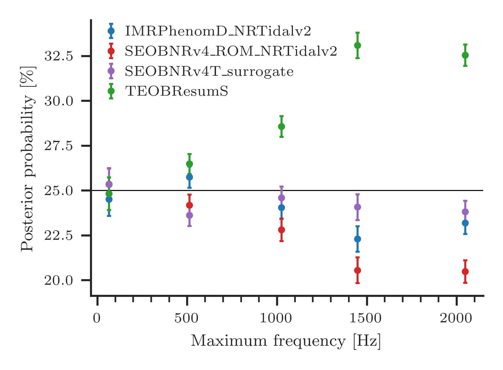
Figure 2: The evolution of the posterior probability of each waveform for GW170817 as the maximum frequency of the analysis data is varied.

4 Conclusion

In this work, we present a hypermodel approach to analysing binary neutron star mergers which (i) provides “on the fly” marginalised posteriors distribution for gravitational-wave studies that reduce potential systematic effects from gravitational-wave models; (ii) allows for model selection of gravitational-wave approximants; (iii) tests gravitational-wave model assumptions without computationally expensive numerical-relativity simulations. We apply this approach to the two confidently detected binary neutron star collisions, GW170817 and GW190425 and the sub-threshold candidate GW200311_103121. We find a consistent preference for the TEOBResumS waveform model with an overall odds that ranges from 2.3 against SEOBNRv4_ROM_NRTidalv2 to 1.7 against IMRPhenomD_NRTidalv2 These odds fall short of substantial evidence, but the consistency between the events suggests that TEOBResumS is subtly better at explaining the observed data. Identifying such a subtlety is essential. Future observing runs of the LIGO, Virgo, and KAGRA detectors will be more sensitive thanks to developments in instrumentation. This sensitivity translates into a greater clarity with which we observe events and hence, improved constraints on fundamental physics along with an increase in the number of detections[51]. Therefore, future data will be critical to determine if TEOBResumS is better at predicting the data. However, we anticipate that all models considered herein will be further improved before the next observing run. We encourage the waveform modelling community to validate new developments by rerunning the analyses in this work, potentially also by using numerical-relativity based injection data.

5 Method

The source properties of gravitational-wave signals observed by ground-based interferometers are inferred using stochastic sampling[46, 52, 53, 54, 14]. Applying a Bayesian approach, the goal of sampling is to to approximate the posterior probability distribution

$$p(\bm{\theta}|\mathbf{d},\Omega)\propto\mathcal{L}(\mathbf{d}|\bm{\theta},\Omega)\pi(\bm{\theta}|\Omega)\,,$$ (2)

where $\bm{\theta}$ is a vector of the model parameters (e.g., the mass and spin of the binary components), $\mathbf{d}$ is the time series of strain data recorded by the interferometer, $\Omega$ is the waveform approximant, $\mathcal{L}$ is the likelihood of the data given $\Omega$ and $\theta$, and $\pi$ is the prior probability density for $\theta$ given $\Omega$. Typically, a stochastic sampler produces an approximation of the posterior by generating a set of independent samples $\{\theta_{i}\}$ drawn from the posterior, which can be used, e.g., to calculate summary statistics.

In addition to the posterior, stochastic sampling can also approximate the Bayesian evidence $\mathcal{Z}(\mathbf{d}|\Omega)$ which is fundamental to the notion of model comparison. Given multiple waveform approximant models, say $\Omega_{A}$ and $\Omega_{B}$, robust measurements of the evidence can enable a model comparison via the Bayesian odds:

$$\underbrace{\mathcal{O}_{A/B}}_{P(\Omega_{A}|\mathbf{d})/P(\Omega_{B}|\mathbf{d})}=\underbrace{\rm BF_{A/B}}_{\mathcal{Z}(\mathbf{d}|\Omega_{A})/\mathcal{Z}(\mathbf{d}|\Omega_{B})}\times\underbrace{\pi_{A/B}}_{\pi(\Omega_{A})/\pi(\Omega_{B})}\,.$$ (3)

The odds $\mathcal{O}_{A/B}$ are the relative probability of two models given the data and are calculated from the product of the data-driven Bayes factor $\rm BF_{A/B}$, and the prior-odds $\pi_{A/B}$. Typically, we have no prior preference between models such that $\pi_{A/B}=1$ and the odds and Bayes factor are identical.

Two stochastic sampling approaches have been demonstrated[55, 56] to be capable of robustly inferring both the posterior distribution and evidence of a gravitational-wave signal: Markov-Chain Monte-Carlo (MCMC)[57, 58] and Nested Sampling[35]. In addition to MCMC and Nested Sampling, there are also grid-based approaches [59, 60] which employ massive parallelisation and iterative fitting. With appropriate tuning, both MCMC and Nested Sampling algorithms are roughly equally capable of approximating the posterior density. However, Nested Sampling is more efficient in calculating the Bayesian evidence[46, 61]. Therefore, the Nested Sampling approach is typically favoured in model selection problems.

However, calculating the odds between two models is only part of the problem. Typically, several models are available, and often they are nearly equally favoured when confronted with observations[31, 62, 63, 64]. As a result, when drawing astrophysical conclusions from an event, it is essential to capture the systematic modelling uncertainty to avoid biased inferences. Results published so far by the LIGO-Scientific and Virgo Collaborations have addressed this issue by combining equal numbers of samples from a subset of pre-selected waveform models[52, 53, 54, 14]. In effect, this presupposes that all waveform models are equally successfully at predicting the data. However, this is certainly not the case and hence discards information about how well each model predicts the data. An alternative approach[34], demonstrated how the Bayesian evidence can be used to capture this additional information, weighting samples and producing a set of posterior samples that marginalises over the pre-selected waveform models. Subsequently, it was demonstrated[36] how the grid-based approaches[60] could be extended to perform model comparisons between pre-selected waveforms. However, rather than calculating the Bayesian evidence, this approach instead included multiple models in the likelihood itself.

In this work, we introduce a new approach to calculating the odds between waveform approximants and calculating posteriors marginalised over a set of $n$ waveform models. First, we extend the definition of the traditional waveform model to a hypermodel $\Omega\rightarrow\Omega=\{\Omega_{0},\Omega_{1},\ldots\Omega_{n-1}\}$; when sampling we then infer the properties of the parameter set $\{\bm{\theta},\omega\}$ where $\bm{\theta}$ is the usual vector of astrophysical model parameters while $\omega$ is a categorical waveform-approximant parameter $\omega\in[0,1,2,\ldots,n-1]$. We apply an uninformative prior on $\omega$, $\pi(\omega)=1/n$. Then, at each iteration of the MCMC sampler, following the standard Metropolis-Hastings algorithm[57, 58], a new point in the set of model parameters is proposed, including a proposal for the categorical waveform model. Given the proposed point, we first apply a pre-determined mapping between $\omega$ and the set of waveform approximants under study to select which waveform to use. Then, the likelihood is calculated according to the remaining model parameters. We implement the categorical approach in the Bilby-MCMC sampler. The only additional step is the addition of a specialised proposal routine for the categorical variable $\omega$, here we use a random draw from the prior.

It is worth pointing out that the MCMC-hypermodel approach does not add any additional computational cost compared to separate MCMC analyses. One can quantify this by looking at the autocorrelation time $\tau$, which determines the number of steps required for the MCMC to produce a fixed number of independent samples[65]. Comparing an MCMC-hypermodel analysis with four waveforms to an identical analysis with a single waveform, we find that $\tau$ only differs by the expected uncertainty due to sampling, i.e., the addition of the hypermodel parameter does not increase $\tau$. This is because $\tau$ is taken as the maximum over all parameters; for the analyses presented here, the autocorrelation time of difficult-to-sample-parameters, such as the mass ratio, dominate, while the hypermodel parameter $\omega$ demonstrates good mixing and hence does not increase the maximum $\tau$. The computational cost of the analysis is directly proportional to $\tau$[61]. Therefore, the total computational cost of running the four waveforms separately is nearly four times larger then running them together in the hyper-model approach if one only requires the same number of combined (waveform-marginalized) samples for the hypermodel approach compared to each individual run. However, this is not a fair comparison, since one only obtains a quarter of the number of samples per waveform compared to running four individual analyses. A fairer comparison is to require the same number of samples per waveform model. Then, the two approaches have a near identical computational cost, with the hypermodel approach marginally more efficient because the MCMC burn-in cost is only paid once. However, this does not hold if one model is strongly favoured. In this case, the autocorrelation time of the hypermodel approach may be dominated by the waveform mixing and there are inefficiencies in running the sampler for a long duration to produce a fixed number of samples for the worst performing model. For these reasons, and arguments below, we suggest a Nested Sampling approach instead be applied when one model is strongly preferred.

The MCMC-hypermodel approach applied in this work is a special case of the Reversible-Jump MCMC (RJMCMC) algorithm[66] which enables the models to differ in the model parameters. In this work, we consider only models with identically-defined parameters $\bm{\theta}$. Hence, we distinguish our hypermodel approach from the RJMCMC algorithm. However, in future work we hope to extend the sampling algorithm to a full RJMCMC sampler. This will enable the comparison of waveform models with differing nature, e.g., one could compare binary neutron star, neutron-star black-hole, and binary black hole models directly, or in comparing precessing and aligned-spin models. The RJMCMC algorithm has been applied in other contexts in gravitational-wave data analysis before, e.g., for unmodelled searches[67, 68], power-spectral density estimation[43], and population inferences[69].

Running the MCMC-hypermodel sampler on $n$ waveform approximants, we obtain a set of $N$ independent samples from the posterior $\{\theta_{i}\}$. By design, these samples are mixed according to the relative posterior probability of the individual waveform models. Individual posterior distributions for each waveform approximant can be obtained by filtering the posterior against the relevant $\omega$ index. The probability of the $\ell$-th waveform approximant relative to all other waveform approximants considered in the categorical analysis is $p_{\ell}=n_{\ell}/N$. Finally, the Bayesian odds between two models ($\omega=A$ and $\omega=B$) is given by

$$\mathcal{O}_{A/B} =\frac{p_{A}}{p_{B}}\,,$$ (4)

with an estimated variance:

$$\sigma_{\mathcal{O}_{A/B}}^{2} \approx\frac{\mathcal{O}_{A/B}^{2}}{N}\left(\frac{1}{p_{A}}+\frac{1}{p_{B}}\right)\,.$$ (5)

If only two models are under consideration, this demonstrates that at leading order $\sigma_{\mathcal{O}_{A/B}}^{2}\approx\mathcal{O}_{A/B}^{2}/N$. At fixed $N$, the variance has a minimum when $\mathcal{O}_{A/B}=1$, i.e., the method is best-suited to study cases where $\mathcal{O}\sim 1$, but the uncertainty grows with the odds. For cases where the odds strongly favour one model over the other, $N$ can be increased to achieve a fixed level of uncertainty. But, in cases where the odds are strongly informative (i.e., $\mathcal{O}\gg 1$ or $\mathcal{O}\ll 1$), a Nested Sampling approach will be more efficient. For Nested Sampling, the evidence is estimated for each model individually and the uncertainty is independent of the odds. Nested Sampling is therefore well suited to estimating odds for clear-cut model comparisons. However, for cases where the models are in close contention, the scaling of the uncertainty with $N$ makes the MCMC approach preferable. For example, while we use standard settings[61] for both the MCMC and Nested Sampling methods, the uncertainties reported in Table 1 are nearly an order of magnitude larger for the Nested Sampling odds than that of the MCMC approach. We could reduce the uncertainty on the Nested Sampling odds by changing the stopping criteria of the sampler with a corresponding increase in the computational cost. While a detailed study of computational efficiency of the two approaches is beyond the scope of this analysis, we note here that the total number of CPU days was approximately 400 for the MCMC-hypermodel analysis of GW170817 while it was 350 for the Nested Sampling analysis illustrating that at a similar level of computing cost, the MCMC method outperforms the Nested Sampling approach when $\mathcal{O}\sim 1$. (Note: all timing performed on Intel 2.4 GHz Gold 6148 CPUs).

The prior-odds, $\pi_{A/B}$, enter via the prior on the categorical waveform-approximant parameter $\pi(\omega)$. For our uninformative choice above, $\pi_{A/B}=1$. But, if cogent prior information about the models is available, this can be included in the prior on $\omega$.

6 Supplementary Material

6.1 Interpreting the Odds

In this work, we discuss the odds between different waveform models of binary neutron star collisions. We find that the odds are in favour (i.e. greater than unity) of the TEOBResumS waveform model across multiple events. The consistency of this finding means that when we combine the odds, we end up with an odds ranging from 1.7 to 2.3 with an uncertainty of $\sim 0.2$. In this Appendix, we discuss the interpretation of this using a simple toy model for demonstration.

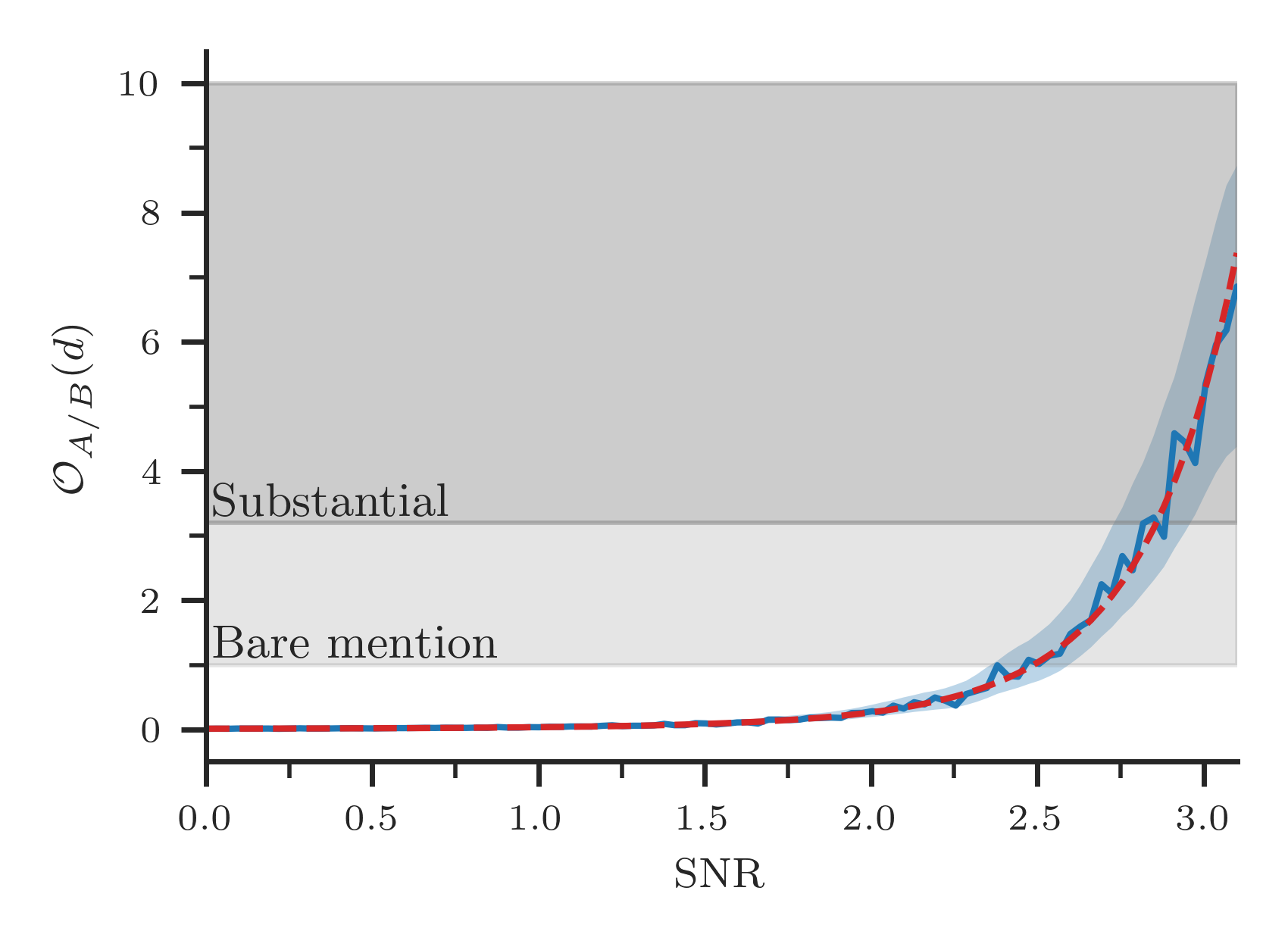
Figure 3: The odds as a function of the SNR ($\mu/\sigma$) for our toy model as predicted by Eq. 3 (red dashed lines) and by Nested Sampling (blue solid line) and the 3 standard-deviation uncertainty on the Nested Sampling odds (light blue shaded band). In gray bands, we show common thresholds for interpretation of the Odds[48].

The Odds, quantify the ratio of probabilities of two models given data (see, e.g. Eq. 3). Often, the reader will want to interpret this quantitative statement. To this end, interpretative thresholds have been defined. One popular approach[48], which builds on Jeffrey’s foundational work[70], suggests that an odds in the range of 1-3.2 is “not worth more than a bare mention” while 3.2-10 is “substantial evidence“. Such a categorisation is useful in ensuring consistency in standards of evidence in scientific investigations. However, there are several caveats to keep in mind. First, as noted by the authors, the interpretations should depend on the context. E.g., one may desire a more stringent interpretation for forensic evidence in a criminal trial than other contexts. Second, the uncertainty on the evidence plays an important role. If the odds are consistent with unity (to within the stated uncertainty), then no preference between the models can be inferred: we must be able to confidently rule out an odds of unity to have any meaningful result. Finally, applying blindly the (somewhat arbitrary) thresholds of any particular interpretative table disregards that the odds are (typically) smooth functions of the strength of the evidence.

To put these points in context, we consider a simple toy model consisting of data $d=\mu+\epsilon$ where $\epsilon$ is the noise drawn from a zero-mean normal distribution with variance $\sigma^{2}$ and $\mu$ is the mean. Then, we define two models, model A, where $\mu$ is an unknown parameter to be marginalized over, and model B where $\mu=0$. Given observed data $d$, the odds of model A vs B (assuming equal prior-odds) are

$$\mathcal{O}_{A/B}(d)\approx\frac{\sigma\sqrt{2\pi}}{\mu_{\rm max}-\mu_{\rm min}}e^{d^{2}/2\sigma^{2}}\,$$ (6)

where $[\mu_{\rm min},\mu_{\rm max}]$ is the prior range and assumed to be wide with respect to the posterior distribution on $\mu$. Defining $\sigma/\mu$ as the signal-to-noise ratio (SNR), then in the limit SNR$\gg 1$, we recover the familiar result $\ln\mathcal{O}_{A/B}\sim\textrm{SNR}^{2}$. To simulate our practical settings, in which we cannot calculate the odds in closed form, we estimate the odds using Nested Sampling and plot the results along with the prediction of Eq. 6 in Fig. 3. The use of Nested Sampling to approximate the evidence naturally yields a quantified uncertainty on the odds which we plot as a shaded band.

Fig. 3 demonstrates the final two caveats that we noted above: the uncertainty inherent in estimated odds blurs the sharp boundaries and, regardless of any threshold-based interpretive table, the odds are still a smooth function of the strength of the evidence. The importance of this for the present work is exemplified by the distinct region in Fig. 3 in which the odds are distinct from unity (in the sense that the lower bound on the odds is larger than 1), but do not rise to the level of “substantial”. How then should be interpret such a result? Clearly this is not “substantial” evidence, but discarding the result seems to ignore that we can confidently exclude an odds of unity. In this work, we choose to interpret this as “marginal evidence”.

Finally, we come back to the first caveat, the context. With the next observing run of the international network of gravitational wave detectors expected in the coming years, it is likely that we will see several binary neutron star mergers. If just two or three of these are as loud as GW170817, they may provide sufficient enough evidence for the joint odds to reach the level of substantial evidence. However, in the meantime, we anticipate that waveform modellers will improve their model in anticipation of the new observations. As such, the marginal evidence reported here may be of critical use in determining which aspects of their models to improve!

6.2 Posterior distributions for GW190425 and GW200311_103121

Posterior distributions for GW190425 and GW200311_103121 are presented in Fig. 4 and Fig. 5, respectively.

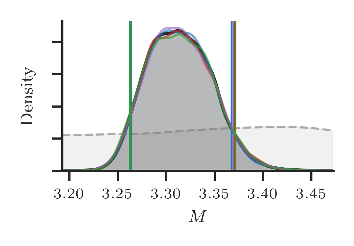
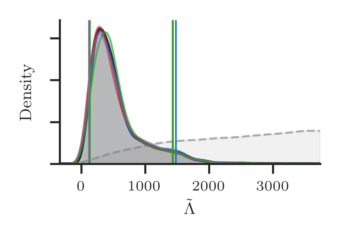
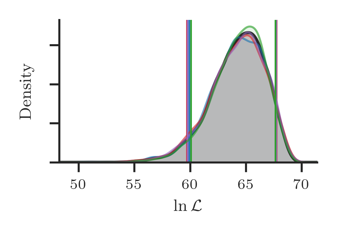
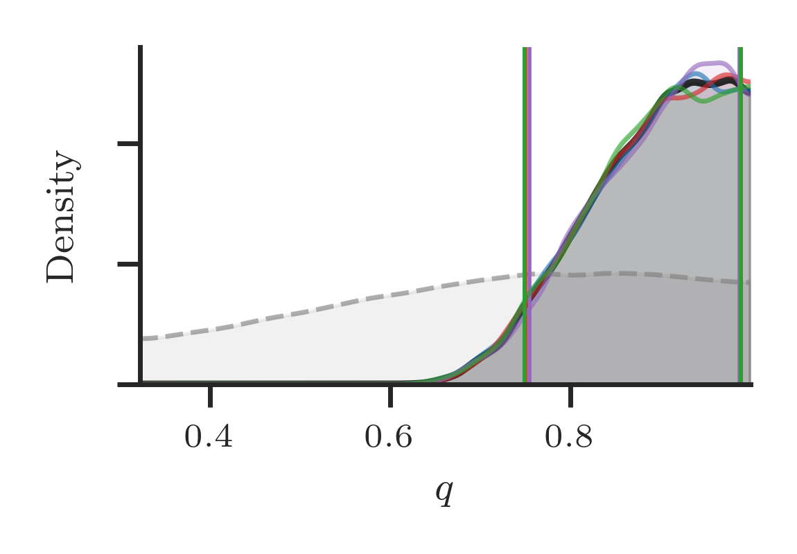
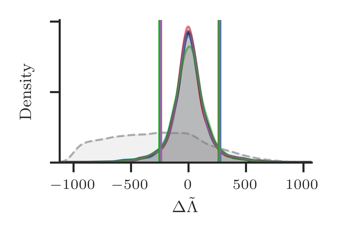
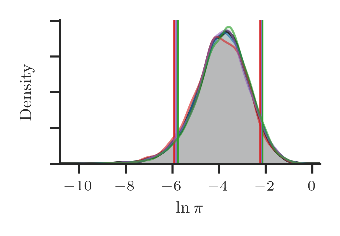
Figure 4: Posterior densities for the mass and tidal deformability of GW190425. We show the combined posteriors, marginalized over all waveform models using the hypermodel approach, and the posteriors for each individual model, extracted from the combined posterior, as well. The dashed curve provides the prior distribution estimated by drawing samples. In the right-hand column, we include the distributions of the log-likelihood and log-prior of the posterior samples.

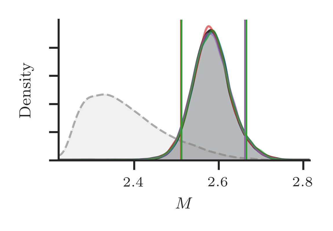
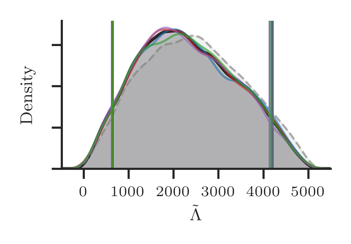
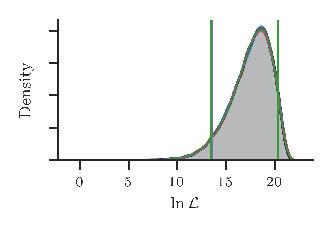
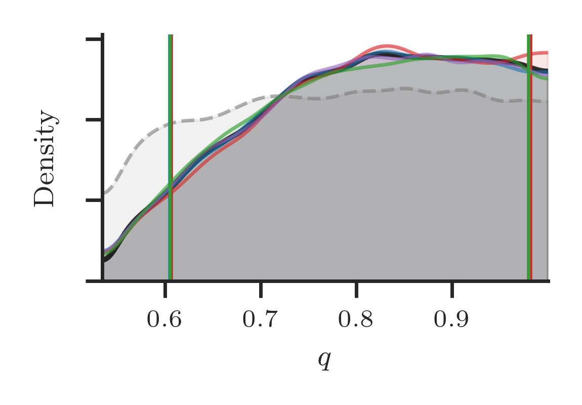
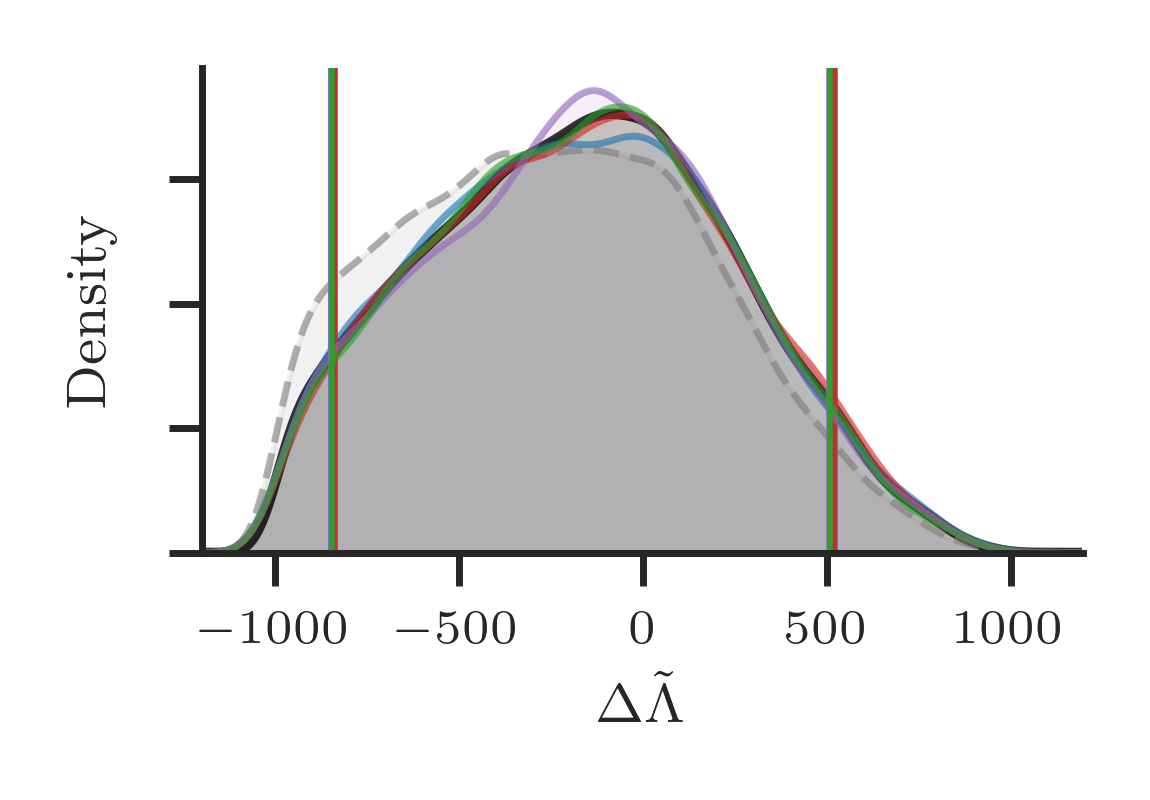
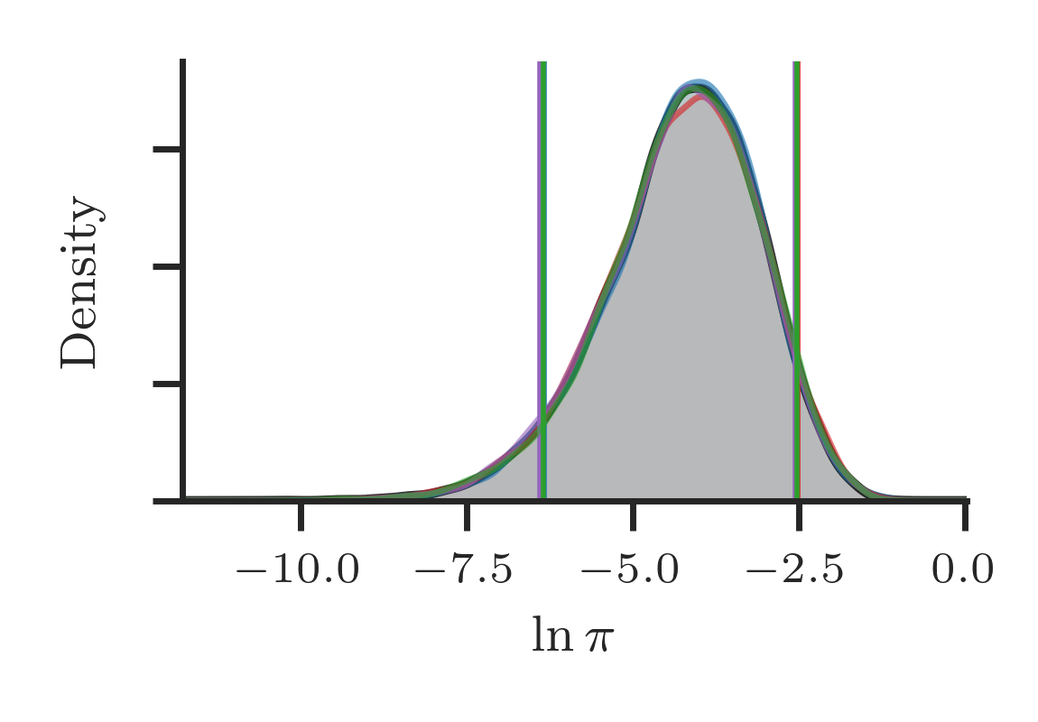
Figure 5: Posterior densities for the mass and tidal deformability of GW200311_103121. We show the combined posteriors, marginalized over all waveform models using the hypermodel approach, and the posteriors for each individual model, extracted from the combined posterior, as well. The dashed curve provides the prior distribution estimated by drawing samples. In the right-hand column, we include the distributions of the log-likelihood and log-prior of the posterior samples.

7 Data Availability

The results for the primary analyses of GW170817, GW190425, and GW200311_103121 are available in the data release[71].

8 Code Availability

The program for the primary analyses of GW170817, GW190425, and GW200311_103121 is described and available in the data release[71].

9 Acknowledgements

We thank Sarp Akcay for valuable comments on the manuscript and comments about the tidal sector of the TEOBResumS model. We are also grateful for discussions with Sebastiano Bernuzzi, Rosella Gamba, and Alessandro Nagar. Finally, we thank Jacopo Tissino for pointing out a mistake in Equation 5 in an early draft of this work. All Nested Sampling analyses made use of the dynesty package[72] and the higher-order mode analysis of TEOBResumS additionally used the massively-parallelised software parallel_bilby[73]. GA thanks the UKRI Future Leaders Fellowship for support through the grant MR/T01881X/1. TD thanks the Max Planck Society for financial support. We are grateful for computational resources provided by Cardiff University, and funded by an STFC grant ST/I006285/1 supporting UK Involvement in the Operation of Advanced LIGO. This work makes use of the scipy[74] and numpy[75, 76, 77] packages for data analysis and visualisation.

10 Author contributions

Conceptualisation: GA, TD; Methodology: GA, TD; Data curation: GA; Software: GA; Validation: GA, TD; Formal analysis: GA; Resources: GA, TD; Funding acquisition: GA, TD; Project administration: GA, TD; Supervision: GA, TD; Visualisation: GA; Writing–original draft: GA, TD; Writing–review and editing: GA, TD.

11 Competing interests

The authors declare that they have no competing financial interests.

12 Correspondence

gregory.ashton@ligo.org

References

- [1] Abbott, B. P. et al. GW170817: Observation of Gravitational Waves from a Binary Neutron Star Inspiral. Phys. Rev. Lett. 119, 161101 (2017). 1710.05832.
- [2] Abbott, B. P. et al. A gravitational-wave standard siren measurement of the Hubble constant. Nature, 10.1038/nature24471 (2017). 1710.05835.
- [3] Hotokezaka, K. et al. A Hubble constant measurement from superluminal motion of the jet in GW170817. Nature Astron. (2019). 1806.10596.
- [4] Dietrich, T. et al. Multimessenger constraints on the neutron-star equation of state and the Hubble constant. Science 370, 1450–1453 (2020). 2002.11355.
- [5] Cowperthwaite, P. S. et al. The Electromagnetic Counterpart of the Binary Neutron Star Merger LIGO/Virgo GW170817. II. UV, Optical, and Near-infrared Light Curves and Comparison to Kilonova Models. Astrophys. J. 848, L17 (2017). 1710.05840.
- [6] Smartt, S. J. et al. A kilonova as the electromagnetic counterpart to a gravitational-wave source. Nature, 10.1038/nature24303 (2017). 1710.05841.
- [7] Kasliwal, M. M. et al. Illuminating Gravitational Waves: A Concordant Picture of Photons from a Neutron Star Merger. Science 358, 1559 (2017). 1710.05436.
- [8] Kasen, D., Metzger, B., Barnes, J., Quataert, E. & Ramirez-Ruiz, E. Origin of the heavy elements in binary neutron-star mergers from a gravitational wave event. Nature, 10.1038/nature24453 (2017). 1710.05463.
- [9] Ezquiaga, J. M. & Zumalacárregui, M. Dark Energy After GW170817: Dead Ends and the Road Ahead. Phys. Rev. Lett. 119, 251304 (2017). 1710.05901.
- [10] Baker, T. et al. Strong constraints on cosmological gravity from GW170817 and GRB 170817A. Phys. Rev. Lett. 119, 251301 (2017). 1710.06394.
- [11] Creminelli, P. & Vernizzi, F. Dark Energy after GW170817 and GRB170817A. Phys. Rev. Lett. 119, 251302 (2017). 1710.05877.
- [12] Multi-messenger Observations of a Binary Neutron Star Merger. Astrophys. J. 848, L12 (2017). 1710.05833.
- [13] Abbott, B. P. et al. GW190425: Observation of a Compact Binary Coalescence with Total Mass . Astrophys. J. Lett. 892, L3 (2020). 2001.01761.
- [14] Abbott, R. et al. GWTC-3: Compact Binary Coalescences Observed by LIGO and Virgo During the Second Part of the Third Observing Run (2021). 2111.03606.
- [15] Brügmann, B. Fundamentals of numerical relativity for gravitational wave sources. Science 361, 366–371 (2018). URL https://science.sciencemag.org/content/361/6400/366. https://science.sciencemag.org/content/361/6400/366.full.pdf.
- [16] Dietrich, T. et al. CoRe database of binary neutron star merger waveforms. Class. Quant. Grav. 35, 24LT01 (2018). 1806.01625.
- [17] Kiuchi, K., Kawaguchi, K., Kyutoku, K., Sekiguchi, Y. & Shibata, M. Sub-radian-accuracy gravitational waves from coalescing binary neutron stars in numerical relativity. II. Systematic study on the equation of state, binary mass, and mass ratio. Phys. Rev. D 101, 084006 (2020). 1907.03790.
- [18] Aasi, J. et al. Advanced LIGO. Class. Quant. Grav. 32, 074001 (2015). 1411.4547.
- [19] Acernese, F. et al. Advanced Virgo: a second-generation interferometric gravitational wave detector. Class. Quant. Grav. 32, 024001 (2015). 1408.3978.
- [20] Blanchet, L. Gravitational Radiation from Post-Newtonian Sources and Inspiralling Compact Binaries. Living Rev. Relativity 17, 2 (2014). 1310.1528.
- [21] Buonanno, A. & Damour, T. Effective one-body approach to general relativistic two- body dynamics. Phys. Rev. D59, 084006 (1999). gr-qc/9811091.
- [22] Buonanno, A. & Damour, T. Transition from inspiral to plunge in binary black hole coalescences. Phys. Rev. D62, 064015 (2000). gr-qc/0001013.
- [23] Dietrich, T., Bernuzzi, S. & Tichy, W. Closed-form tidal approximants for binary neutron star gravitational waveforms constructed from high-resolution numerical relativity simulations. Phys. Rev. D96, 121501 (2017). 1706.02969.
- [24] Bernuzzi, S., Nagar, A., Dietrich, T. & Damour, T. Modeling the Dynamics of Tidally Interacting Binary Neutron Stars up to the Merger. Phys.Rev.Lett. 114, 161103 (2015). 1412.4553.
- [25] Hotokezaka, K., Kyutoku, K., Okawa, H. & Shibata, M. Exploring tidal effects of coalescing binary neutron stars in numerical relativity. II. Long-term simulations. Phys. Rev. D91, 064060 (2015). 1502.03457.
- [26] Hinderer, T. et al. Effects of neutron-star dynamic tides on gravitational waveforms within the effective-one-body approach. Phys. Rev. Lett. 116, 181101 (2016). 1602.00599.
- [27] Dietrich, T. et al. Improving the NRTidal model for binary neutron star systems. Phys. Rev. D100, 044003 (2019). 1905.06011.
- [28] Kawaguchi, K. et al. Frequency-domain gravitational waveform models for inspiraling binary neutron stars. Phys. Rev. D97, 044044 (2018). 1802.06518.
- [29] Dudi, R. et al. Relevance of tidal effects and post-merger dynamics for binary neutron star parameter estimation. Phys. Rev. D 98, 084061 (2018). 1808.09749.
- [30] Samajdar, A. & Dietrich, T. Waveform systematics for binary neutron star gravitational wave signals: effects of the point-particle baseline and tidal descriptions. Phys. Rev. D98, 124030 (2018). 1810.03936.
- [31] Gamba, R., Breschi, M., Bernuzzi, S., Agathos, M. & Nagar, A. Waveform systematics in the gravitational-wave inference of tidal parameters and equation of state from binary neutron star signals. Phys. Rev. D 103, 124015 (2021). 2009.08467.
- [32] Pratten, G., Schmidt, P. & Williams, N. Impact of Dynamical Tides on the Reconstruction of the Neutron Star Equation of State (2021). 2109.07566.
- [33] Kunert, N., Pang, P. T. H., Tews, I., Coughlin, M. W. & Dietrich, T. Quantifying modelling uncertainties when combining multiple gravitational-wave detections from binary neutron star sources (2021). 2110.11835.
- [34] Ashton, G. & Khan, S. Multiwaveform inference of gravitational waves. Phys. Rev. D 101, 064037 (2020). 1910.09138.
- [35] Skilling, J. Nested sampling for general Bayesian computation. Bayesian Analysis 1, 833–859 (2006).
- [36] Jan, A. Z., Yelikar, A. B., Lange, J. & O’Shaughnessy, R. Assessing and marginalizing over compact binary coalescence waveform systematics with RIFT. Phys. Rev. D 102, 124069 (2020). 2011.03571.
- [37] Husa, S. et al. Frequency-domain gravitational waves from nonprecessing black-hole binaries. I. New numerical waveforms and anatomy of the signal. Phys. Rev. D93, 044006 (2016). 1508.07250.
- [38] Khan, S. et al. Frequency-domain gravitational waves from nonprecessing black-hole binaries. II. A phenomenological model for the advanced detector era. Phys. Rev. D93, 044007 (2016). 1508.07253.
- [39] Bohé, A. et al. Improved effective-one-body model of spinning, nonprecessing binary black holes for the era of gravitational-wave astrophysics with advanced detectors. Phys. Rev. D95, 044028 (2017). 1611.03703.
- [40] Lackey, B. D., Pürrer, M., Taracchini, A. & Marsat, S. Surrogate model for an aligned-spin effective one body waveform model of binary neutron star inspirals using Gaussian process regression. Phys. Rev. D100, 024002 (2019). 1812.08643.
- [41] Nagar, A. et al. Time-domain effective-one-body gravitational waveforms for coalescing compact binaries with nonprecessing spins, tides and self-spin effects. Phys. Rev. D98, 104052 (2018). 1806.01772.
- [42] Abbott, B. P. et al. Properties of the binary neutron star merger GW170817. Phys. Rev. X9, 011001 (2019). 1805.11579.
- [43] Littenberg, T. B. & Cornish, N. J. Bayesian inference for spectral estimation of gravitational wave detector noise. Phys. Rev. D 91, 084034 (2015). 1410.3852.
- [44] Payne, E., Talbot, C., Lasky, P. D., Thrane, E. & Kissel, J. S. Gravitational-wave astronomy with a physical calibration model. Phys. Rev. D 102, 122004 (2020). 2009.10193.
- [45] Abbott, B. P. et al. GW170817: Observation of Gravitational Waves from a Binary Neutron Star Inspiral. Phys. Rev. Lett. 119, 161101 (2017). 1710.05832.
- [46] Veitch, J. et al. Parameter estimation for compact binaries with ground-based gravitational-wave observations using the LALInference software library. Phys. Rev. D91, 042003 (2015). 1409.7215.
- [47] Flanagan, E. E. & Hinderer, T. Constraining neutron star tidal Love numbers with gravitational wave detectors. Phys.Rev. D77, 021502 (2008). 0709.1915.
- [48] Kass, R. E. & Raftery, A. E. Bayes Factors. J. Am. Statist. Assoc. 90, 773–795 (1995).
- [49] Harry, I. & Hinderer, T. Observing and measuring the neutron-star equation-of-state in spinning binary neutron star systems. Class. Quant. Grav. 35, 145010 (2018). 1801.09972.
- [50] Dietrich, T., Ujevic, M., Tichy, W., Bernuzzi, S. & Brügmann, B. Gravitational waves and mass ejecta from binary neutron star mergers: Effect of the mass-ratio. Phys. Rev. D95, 024029 (2017). 1607.06636.
- [51] Abbott, B. P. et al. Prospects for observing and localizing gravitational-wave transients with Advanced LIGO, Advanced Virgo and KAGRA. Living Rev. Rel. 23, 3 (2020).
- [52] Abbott, B. P. et al. GWTC-1: A Gravitational-Wave Transient Catalog of Compact Binary Mergers Observed by LIGO and Virgo during the First and Second Observing Runs. Phys. Rev. X9, 031040 (2019). 1811.12907.
- [53] Abbott, R. et al. GWTC-2: Compact Binary Coalescences Observed by LIGO and Virgo During the First Half of the Third Observing Run. Phys. Rev. X 11, 021053 (2021). 2010.14527.
- [54] Abbott, R. et al. GWTC-2.1: Deep Extended Catalog of Compact Binary Coalescences Observed by LIGO and Virgo During the First Half of the Third Observing Run (2021). 2108.01045.
- [55] Christensen, N. & Meyer, R. Markov chain Monte Carlo methods for Bayesian gravitational radiation data analysis. Phys. Rev. D 58, 082001 (1998).
- [56] Veitch, J. & Vecchio, A. A Bayesian approach to the follow-up of candidate gravitational wave signals. Phys. Rev. D 78, 022001 (2008). 0801.4313.
- [57] Metropolis, N., Rosenbluth, A. W., Rosenbluth, M. N., Teller, A. H. & Teller, E. Equation of state calculations by fast computing machines. J. Chem. Phys. 21, 1087–1092 (1953).
- [58] Hastings, W. K. Monte Carlo Sampling Methods Using Markov Chains and Their Applications. Biometrika 57, 97–109 (1970).
- [59] Pankow, C., Brady, P., Ochsner, E. & O’Shaughnessy, R. Novel scheme for rapid parallel parameter estimation of gravitational waves from compact binary coalescences. Phys. Rev. D92, 023002 (2015). 1502.04370.
- [60] Lange, J., O’Shaughnessy, R. & Rizzo, M. Rapid and accurate parameter inference for coalescing, precessing compact binaries (2018). 1805.10457.
- [61] Ashton, G. & Talbot, C. Bilby-MCMC: An MCMC sampler for gravitational-wave inference (2021). 2106.08730.
- [62] Estellés, H. et al. A detailed analysis of GW190521 with phenomenological waveform models (2021). 2105.06360.
- [63] Mateu-Lucena, M. et al. Adding harmonics to the interpretation of the black hole mergers of GWTC-1 (2021). 2105.05960.
- [64] Colleoni, M. et al. Towards the routine use of subdominant harmonics in gravitational-wave inference: Reanalysis of GW190412 with generation X waveform models. Phys. Rev. D 103, 024029 (2021). 2010.05830.
- [65] Hogg, D. W. & Foreman-Mackey, D. Data analysis recipes: Using Markov Chain Monte Carlo. Astrophys. J. Suppl. 236, 11 (2018). 1710.06068.
- [66] Green, P. J. Reversible jump Markov chain Monte Carlo computation and Bayesian model determination. Biometrika 82, 711–732 (1995).
- [67] Cornish, N. J. & Littenberg, T. B. Tests of Bayesian Model Selection Techniques for Gravitational Wave Astronomy. Phys. Rev. D 76, 083006 (2007). 0704.1808.
- [68] Cornish, N. J. & Littenberg, T. B. BayesWave: Bayesian Inference for Gravitational Wave Bursts and Instrument Glitches. Class. Quant. Grav. 32, 135012 (2015). 1410.3835.
- [69] Farr, W. M. et al. The Mass Distribution of Stellar-Mass Black Holes. Astrophys. J. 741, 103 (2011). 1011.1459.
- [70] Jeffreys, H. The theory of probability (OUP Oxford, 1998).
- [71] Ashton, G. Data release: Understanding binary neutron star collisions with hypermodels (2021). URL https://doi.org/10.5281/zenodo.5707911.
- [72] Speagle, J. S. dynesty: a dynamic nested sampling package for estimating Bayesian posteriors and evidences. Mon. Not. Roy. Astron. Soc. 493, 3132–3158 (2020). 1904.02180.
- [73] Smith, R. J. E., Ashton, G., Vajpeyi, A. & Talbot, C. Massively parallel Bayesian inference for transient gravitational-wave astronomy. Mon. Not. Roy. Astron. Soc. 498, 4492–4502 (2020). 1909.11873.
- [74] Virtanen, P. et al. SciPy 1.0: Fundamental Algorithms for Scientific Computing in Python. Nature Methods 17, 261–272 (2020).
- [75] Oliphant, T. E. A guide to NumPy, vol. 1 (Trelgol Publishing USA, 2006).
- [76] Van Der Walt, S., Colbert, S. C. & Varoquaux, G. The numpy array: a structure for efficient numerical computation. Computing in Science & Engineering 13, 22 (2011).
- [77] Harris, C. R. et al. Array programming with numpy. Nature 585, 357–362 (2020).