Extracting source properties from binary neutron star gravitational wave signals: effects of the point-particle baseline and tidal description

Waveform systematics for binary neutron star gravitational wave signals: effects of the point-particle baseline and tidal descriptions

Abstract

Gravitational wave (GW) astronomy has consolidated its role as a new observational window to reveal the properties of compact binaries in the Universe. In particular, the discovery of the first binary neutron star coalescence, GW170817, led to a number of scientific breakthroughs as the possibility to place constraints on the equation of state of cold matter at supranuclear densities. These constraints and all scientific results based on them require accurate models describing the GW signal to extract the source properties from the measured signal.

In this article, we study potential systematic biases during the extraction of source parameters using different descriptions for both, the point-particle dynamics and tidal effects. We find that for the considered cases the mass and spin recovery show almost no systematic bias with respect to the chosen waveform model. However, the extracted tidal effects can be strongly biased, where we find generally that Post-Newtonian approximants predict neutron stars with larger deformability and radii than numerical relativity tuned models. Noteworthy, an increase in the Post-Newtonian order in the tidal phasing does not lead to a monotonic change in the estimated properties.

We find that for a signal with strength similar to GW170817, but observed with design sensitivity, the estimated tidal parameters can differ by more than a factor of two depending on the employed tidal description of the waveform approximant. This shows the current need for the development of better waveform models to extract reliably the source properties from upcoming GW detections.

I Introduction

With GW170817, the first detected gravitational wave (GW) signal emitted from a binary neutron star (BNS) coalescence, the LIGO-Virgo Collaboration (LVC) managed to place constraints on the unknown equation of state (EOS) for supranuclear dense matter Abbott et al. (2017). Initiated by this study and results obtained by the source properties extracted from the GW signal a number of groups were able to obtain even tighter bounds on the NS radii and EOS either by the combination of the information obtained from the GWs with electromagnetic observations Radice et al. (2018); Bauswein et al. (2017); Coughlin et al. (2018), or by statistical methods based on a large set of possible EOSs combining GW information with new insights from nuclear physics theory Annala et al. (2018); Most et al. (2018). Also the LVC updated their first analysis Abbott et al. (2017) incorporating the known source location, employing updated waveform approximants, using re-calibrated Virgo data, and starting at a lower frequency threshold. The improved analysis, Refs. Abbott et al. (2018a, b), determined the NS radii to be $11.9^{+1.4}_{-1.4}\rm km$. In addition to the LVC, De et al. De et al. (2018) and Dai et al. Dai et al. (2018) re-analyzed GW170817 with slightly different methods finding overall consistency.

Just from this single detection, it was already possible to show that several proposed nuclear physics EOSs can hardly explain the observed signal Abbott et al. (2017, 2018a, 2018b). The increasing sensitivity of advanced GW detectors over the next years will lead to a growing number of detections of merging BNSs in the near future Abbott et al. (2016) allowing an even more precise measurement of the supranuclear EOSs.

Extracting the source properties of a compact binary from GW data requires Bayesian analysis involving calculation of a multi-dimensional likelihood function of the data with an expected waveform model. In context of the GW data analysis considered in this article, this is done using the Bayesian inference module LALInference Veitch et al. (2015). Consequently, the generation of individual waveforms needs to be efficient to allow evaluation of a large number of templates, but also needs to be accurate enough for a precise measurement of the intrinsic source parameters.

Over the last years, there has been significant progress in the development of BNS waveform approximants capturing the strong-field and tidally dominated regime from the early inspiral up to the merger of the two stars. Exemplary cases for such developments are the improved analytical post-Newtonian (PN) based waveform models, e.g. Damour et al. (2012); Agathos et al. (2015), the existing state-of-the-art tidal waveform models in the time domain as discussed in Bernuzzi et al. (2015); Hotokezaka et al. (2016); Hinderer et al. (2016); Steinhoff et al. (2016); Dietrich and Hinderer (2017); Nagar et al. (2018) based on the effective-one-body (EOB) description of the general-relativistic two-body problem Buonanno and Damour (1999); Damour and Nagar (2010), or closed-form tidal approximants combining PN, tidal EOB, and numerical relativity (NR) information Dietrich et al. (2017, 2018a, 2018b); Kawaguchi et al. (2018). In particular the model of Ref. Dietrich et al. (2017) has proven its importance for the interpretation of GW170817 Abbott et al. (2017, 2018a, 2018b); Dai et al. (2018) due to the significantly smaller computation costs compared to time domain tidal EOB models, but the better accuracy with respect to analytical PN models Dietrich et al. (2018b). Reference Jimenez-Forteza et al. (2018) studied the effects of higher order tidal terms in the PN-expansion in addition to studying the effects of magnetic tidal polarizability and tidal-spin coupling. They concluded that the inclusion of the tidal-tail term at 6.5PN deteriorates the PN series convergence. They also established that the magnetic tidal deformability has negligible effects on the phasing. This has also been studied exclusively in Ref. Pani et al. (2018).

While Ref. Dietrich et al. (2018b) indicated already that NR based waveform models allow more precise and stringent extraction of the source properties, the authors did not perform a full Bayesian analysis to determine the influence of different tidal and point-particle (PP) descriptions on the estimated binary parameters.

The first Bayesian study for the estimation of tidal deformability parameters was carried out in Del Pozzo et al. (2013) which included tidal corrections up to 1PN (6PN in phase). They reported tens of detections required to constrain the tidal deformability parameter to $\sim$ 10% accuracy and distinguish between different types of EOSs by expressing the tidal deformability as a linear expansion in mass. Following this work, Ref. Agathos et al. (2015) extended the analysis including tidal phasing terms up to 2.5PN and modify the termination criterion to be the minimum of the contact frequency Maselli et al. (2013) and the frequency at the last stable orbit (LSO). Their work also included the quadrupole-monopole deformation at leading order Poisson (1998); Yagi and Yunes (2013), which did not affect parameter estimation (PE) for the considered configurations. In addition, the tidal deformability parameter was expanded to include up to a quadratic function of mass. In Lackey and Wade (2015), the pressure and the adiabatic indices were sampled directly. An analytical approach to study the systematic and statistical uncertainties arising from neglecting physical effects in the estimation of the NS Love number was made by Favata (2014), a similar analysis based on a Bayesian approach, was made in Ref. Wade et al. (2014). Very recently, Dudi et al. (2018) investigated NR-based tidal waveform models and showed the importance of the inclusion of tidal effects for the extraction of the NS masses and spins from the GW signal for high signal-to-noise ratios. An exhaustive PE analyses on GW170817-like simulations have been performed in Abbott et al. (2018a) and used the NRTidal description for the first time in PE. The simulations were done with a tidal EOB-based model Hinderer et al. (2016) and the recovery was performed with aligned-spinning models. This work probed different mass-ratios for non-spinning signals all consistent with GW170817-supported EOS models.

Unfortunately, none of the existing works allowed a clear distinction between possible biases introduced by the binary black hole (BBH) or PP description and the particular inclusion of tidal effects. To fill this gap, we study equal and unequal mass BNS signals and employ four different PP baselines and five different tidal descriptions. This allows a systematic study to understand possible biases in the source properties including the tidal parameters.

The article is structured as follows. In Sec. II we discuss the numerical methods and the employed waveform approximants. In Sec. III we assess the imprint of the PP description of the waveform model and in Sec. IV we keep the PP baseline fixed but vary the tidal description. We conclude in Sec. V.

II Numerical settings and waveform models

To determine systematic biases on the extraction of source properties from a detected BNS signal, we simulate a number of waveforms and recover these with waveforms using different combinations of PP baselines and tidal descriptions. New waveform approximants constructed for this article are the IMRPhenomPv2_PNTidal, a combination of IMRP and PN based tidal phasing given by Eq. 4 to IMRPhenomPv2 (henceforth IMRP), and TaylorF2_NRTidal (henceforth TF2NRT), which is a combination of the NRTidal approximation with the TaylorF2 (henceforth TF2) model. Furthermore, we consider the existing PP models IMRPhenomD (IMRD) and SEOBNRv4_ROM (SEOB). Throughout this article, we refer to TF2 extended with PN-tides as TF2PNT, to IMRPhenomPv2_NRTidal as IMRPNRT, to IMRPhenomD_NRTidal as IMRDNRT, and to SEOBNRv4_ROM_NRTidal as SEOBNRT. Details about the BBH baselines and the tidal descriptions are given below.

II.1 Waveform models

Our work is based on four different frequency domain BBH waveform models, summarized in Tab. 1. These baseline models are then extended with different tidal descriptions. All chosen models are fast enough to be used for parameter estimation studies using LALInference and have been employed for the analysis of GW170817 presented in Ref. Abbott et al. (2018a).

The frequency domain waveform is given by

$$\tilde{h}(f)=\tilde{A}(f)e^{-i\Psi(f)},$$ (1)

where the frequency domain phase $\Psi(f)$ can be approximated as a sum of the non-spinning PP contribution, a spin-orbit (SO) contribution, a spin-spin (SS) contribution, and tidal contributions (Tides), i.e.,

$$\Psi(f)=\Psi_{\rm PP}(f)+\Psi_{\rm SO}(f)+\Psi_{\rm SS}(f)+\Psi_{\rm Tides}(f).$$ (2)

II.1.1 BBH-baseline models

Model name	point-particle	spin-orbit	spin-spin	Quadrupole-Monopole	Precession
TaylorF2 (TF2)	3.5PN Sathyaprakash and Dhurandhar (1991)	3.5PN Bohé et al. (2013, 2013)	3PN Arun et al. (2009a); Mikóczi et al. (2005); Bohé et al. (2015); Mishra et al. (2016)	✗ 3PN for BBHs	✗
SEOBNRv4_ROM (SEOB)	EOB model with NR calibration Bohé et al. (2017); Pürrer (2014)			✗ as BBH	✗
IMRPhenomD(IMRD)	phenom. model calibrated to TF2 and EOB/NR-hybrids Husa et al. (2016); Khan et al. (2016); Hannam et al. (2014)			✗ as BBH	✗
IMRPhenomPv2(IMRP)	same spin-aligned model as IMRD			3PN EOS dependentPoisson (1998); Yagi and Yunes (2017)	✓ Schmidt et al. (2012, 2015)

Table 1: Overview about the employed baseline waveform models used in this article.

Let us very briefly review the main characteristics of the underlying BBH models. The TF2 model is a pure analytical PN-based approximant including PP and aligned SO terms to 3.5PN order and SS effects up to 3PN Sathyaprakash and Dhurandhar (1991); Blanchet et al. (1995); Damour et al. (2001); Blanchet et al. (2004, 2005); Bohé et al. (2013); Blanchet (2014); Arun et al. (2009b); Mikoczi et al. (2005); Bohé et al. (2015); Mishra et al. (2016).

The SEOB approximant is a frequency domain reduced order model constructed following Ref. Pürrer (2014) and it is constructed from the aligned-spin EOB model presented in Bohé et al. (2017).

IMRD is based on the aligned-spin model presented in Refs. Husa et al. (2016); Khan et al. (2016) and calibrated to untuned EOB waveforms of Taracchini et al. (2014) and NR hybrids Husa et al. (2016); Khan et al. (2016). Finally, IMRP Hannam et al. (2014) uses IMRD as an underlying spin-aligned approximant which is then ‘twisted up’ to include precession effects as described in Refs. Schmidt et al. (2012, 2015).

II.1.2 Inclusion of tidal effects

To incorporate tidal effects and allow for a proper modeling of BNS waveforms, we employ two different approaches by either including PN-based tidal approximations Vines et al. (2011); Damour et al. (2012) or including an NRTidal approximation Dietrich et al. (2017, 2018a, 2018b) which is calibrated in the high-frequency region to the analytic EOB model of Bernuzzi et al. (2015); Nagar et al. (2018) and NR simulations Dietrich et al. (2017, 2018a, 2018c).

Independent of the exact form of the tidal phase contribution, tidal effects enter the waveform’s phase due to the tidal deformabilities of the individual components in the binary via

$$\Lambda_{A,B}=\frac{2}{3}\frac{k_{2}^{A,B}}{C_{A,B}^{5}},$$ (3)

where $k_{2}^{A,B}$ denote the Love numbers of the individual stars describing the static quadrupolar deformation of one body in the gravitoelectric field of the companion Damour and Nagar (2009), and $C_{A,B}=M_{A,B}/R_{A,B}$ denote the compactness of the individual stars. In terms of the characteristic PN-parameter $x=x(f)=(\pi Mf)^{2/3}$, the PN tidal phase takes the form

$$\Psi_{\rm PNT} =\frac{3}{128\eta x^{5/2}}\Lambda_{A}X_{A}^{4}\left(\underbrace{-24(12-11X_{A})x^{5}}_{\rm 5PN}+\underbrace{\frac{5}{28}(3179-919X_{A}-2286X_{A}^{2}+260X^{3}_{A})x^{6}}_{\rm 6PN}+\underbrace{24\pi(12-11X_{A})x^{6.5}}_{\rm 6.5PN}\right.$$

$$\underbrace{-24\left(\frac{39927845}{508032}-\frac{480043345}{9144576}X_{A}+\frac{9860575}{127008}X_{A}^{2}-\frac{421821905}{2286144}X_{A}^{3}+\frac{4359700}{35721}X_{A}^{4}-\frac{10578445}{285768}X_{A}^{5}\right)x^{7}}_{\rm 7PN^{*}}$$

$$\left.+\underbrace{\frac{\pi}{28}(27719-22127X_{A}+7022X_{A}^{2}-10232X_{A}^{3})x^{7.5}}_{\rm 7.5PN}\right)+[A\leftrightarrow B],$$ (4)

where PN orders marked with ^∗ are incomplete and contain yet unknown parameters which for the analysis of this paper have been set to zero and according to Damour et al. (2012) might be negligible. $X_{A}$ and $X_{B}$ denote respectively the mass fractions $M_{A}/M$ and $M_{B}/M$, $M=M_{A}+M_{B}$ being the total mass of the binary.

For the analyses done with waveform models including the TF2 PP phasing, we have truncated the waveform at a frequency which is the minimum of ISCO or the contact frequency. The latter is given by

$$f_{\mathrm{contact}}=\frac{1}{\pi}\left(\frac{M}{(R(M_{A})+R(M_{B}))^{3}}\right)^{1/2},$$ (5)

where the radii of the component masses are determined using the phenomenological relation between the compactness $C$ and the tidal deformability $\Lambda$ by Maselli et al. (2013)

$$C_{A,B}= 0.371-3.91\times 10^{-2}\ln\Lambda_{A,B}+$$

$$+1.056\times 10^{-3}(\ln\Lambda_{A,B})^{2}.$$ (6)

 

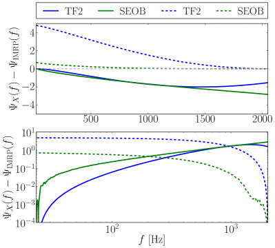
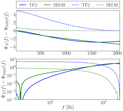
Figure 1: Phase difference between TF2 and SEOB with respect to IMRD for the equal-mass setup (left) and the unequal-mass setup (right). We align the waveforms at $f_{0}=23\ \rm Hz$ (solid lines) and $f_{0}=2048~{}\rm Hz$ (dashed lines) for the equal-mass setup. In the unequal-mass setup, we align the waveforms at $f_{0}=28\ \rm Hz$ (solid lines) and $f_{0}=2048\ \rm Hz$ (dashed lines).

As an alternative approach and as an effective representation of tidal effects beyond the known analytic knowledge, we write the tidal phase as

$$\Psi_{\rm NRT}=-\kappa_{\rm eff}^{T}\frac{c_{\rm Newt}x^{5/2}}{X_{A}X_{B}}P^{\rm NRT}_{\Psi}(x)\ ,$$ (7)

with

$$P^{\rm NRT}_{\Psi}=\frac{1+\tilde{n}_{1}x+\tilde{n}_{3/2}x^{3/2}+\tilde{n}_{2}x^{2}+\tilde{n}_{5/2}x^{5/2}}{1+\tilde{d}_{1}x+\tilde{d}_{3/2}x^{3/2}}$$ (8)

where $x$ is defined above, $\tilde{c}_{\rm Newt}=39/16$ and $\tilde{d}_{1}=\tilde{n}_{1}-3115/1248$. The remaining parameters are determined by fitting and read $(\tilde{n}_{1},\tilde{n}_{3/2},\tilde{n}_{2},\tilde{n}_{5/2})=(-17.428,31.867,-26.414,62.362)$ and $\tilde{d}_{3/2}=36.089$. We have explicitly set $\tilde{d}_{1}=(\tilde{n}_{1}-\tilde{c}_{1})$ to ensure the recovery of the analytic PN knowledge up to 6PN. For details about the calibration procedure, we refer to Refs. Dietrich et al. (2017, 2018b). $\kappa_{\rm eff}^{T}$ is known as the effective tidal coupling constant given by

$$\kappa_{\rm eff}^{T}=\frac{3}{13}\left[X_{A}^{4}\Lambda_{A}\left(12-11X_{A}\right)+(A\leftrightarrow B)\right]$$ (9)

When using waveform models with the Phenom and SEOB PP phasing, we use the termination frequency determined by the tidal coupling constant $\kappa_{2}^{T}$ given by

$$f_{\mathrm{merger}}=\frac{1}{2\pi}\omega_{0}\sqrt{\frac{X_{B}}{X_{A}}}\frac{1+n_{1}\kappa_{2}^{T}+n_{2}(\kappa_{2}^{T})^{2}}{1+d_{1}\kappa_{2}^{T}+d_{2}(\kappa_{2}^{T})^{2}},$$ (10)

with

$$\kappa_{2}^{T}=3X_{A}X_{B}\left[X_{A}^{3}\Lambda_{A}+(A\leftrightarrow B)\right],$$ (11)

where $n_{1}=3.354\times 10^{-2}$, $n_{2}=4.315\times 10^{-5}$, $d_{1}=7.542\times 10^{-2}$ and $d_{2}=2.236\times 10^{-4}$. The parameter $\omega_{0}=0.356$ is chosen such that for $M_{A}=M_{B}$ and $\kappa_{2}^{T}\rightarrow 0$, the non-spinning BBH limit is recovered Dietrich et al. (2018b). The coupling constant $\kappa_{2}^{T}$ is closely related to $\kappa_{\rm eff}^{T}$ and it is indeed the latter which is used in LALSuite.

In addition to the discussed tidal effects which are independent of the NS’ spin, spin effects depending on the EOS of the NSs enter already at 2PN. These spin induced quadrupole-monopole (QM) effects are included in the IMRP up to 3PN. The spin-induced quadrupole moment Poisson (1998) is calculated from the tidal parameter of each NS using the quasi-universal relations of Yagi and Yunes (2017). While in this article the EOS-dependent QM effects are only included in the IMRP and TF2 approximants, this has purely historical reasons. In fact, a new implementation of the SEOBNRT approximant also includes these effects, but was not available when our injection study was started.

II.2 Injection study

	$M_{A}\ [\rm M_{\odot}]$	$M_{B}\ [\rm M_{\odot}]$	$M\ [\rm M_{\odot}]$	$q=\frac{M_{B}}{M_{A}}$	$\Lambda_{A}$	$\Lambda_{B}$	$\tilde{\Lambda}$	$D_{L}\ [\mathrm{Mpc}]$
Source-1	1.375	1.375	2.75	1	292	292	292	50
Source-2	1.68	1.13	2.81	0.67	102.08	840.419	292	50

Table 2: Overview about the injected sources. The columns refer to the individual masses, the total mass, the mass ratio, the individual tidal deformabilities, the effective tidal deformability $\tilde{\Lambda}$ and the luminosity distance to the source. Both sources are non-spinning.

We perform simulations with sources in agreement with the EOS constraints obtained from Refs. Abbott et al. (2018b, a). All simulations are performed in stationary Gaussian noise assuming LIGO and Virgo design sensitivity Abbott et al. (2018c); Adv . For the first source, we choose an equal-mass binary of component mass 1.375 $\mathrm{M}_{\odot}$ and component tidal deformability of $\Lambda_{A}=\Lambda_{B}=292$. To investigate further the effect of mass-ratio on the estimates of tidal deformability, we perform a second set of simulations with $M_{A}=1.68,M_{B}=1.13$ and $\Lambda_{A}=102.08,\Lambda_{B}=840.419$, cf. Tab. 2.

Both sources are at a luminosity distance of $50\ \rm Mpc$ and placed face-on. The right ascension and declination are $60$ degrees each. All considered sources are non-spinning. The effects of spin and precession need an extended set of injection setups and, therefore, a large amount of additional computational resources. Thus, we postpone this analysis to the future. The masses and tidal deformabilities of the sources are summarized in Tab. 2. The inference is performed with a Bayesian approach.

II.2.1 Bayesian inference

We follow a Bayesian approach for parameter estimation, using the built-in inference module LALInference Veitch et al. (2015) in the LALSuite package. The sampling is done with the Markov Chain Monte Carlo (MCMC) algorithm within LALInference, called lalinference_mcmc Rodriguez et al. (2014). In the Bayesian framework, all information about the parameters of interest is encoded in the posterior probability distribution function (PDF) given by Bayes’ theorem:

$$p(\vec{\theta}|\mathcal{H}_{s},d)=\frac{p(\vec{\theta}|\mathcal{H}_{s})p(d|\vec{\theta},\mathcal{H}_{s})}{p(d|\mathcal{H}_{s})},$$ (12)

where $\vec{\theta}$ represents the parameter set and $\mathcal{H}_{s}$ is the hypothesis that a GW signal depending on the parameters $\vec{\theta}$ is present in the data $d$. In our setting, the parameter set consists of the parameters common to a BBH signal $\{M_{A},M_{B},\chi_{A},\chi_{B},\alpha,\delta,\iota,\psi,D_{L},t_{c},\varphi_{c}\}$, and in addition the two tidal deformability parameters $\Lambda_{A}$ and $\Lambda_{B}$ characteristic to a BNS system. Henceforth, we will follow the mass-weighted tidal deformability introduced by, e.g. Flanagan and Hinderer (2008)

$$\tilde{\Lambda}=\frac{16}{13}\sum_{i=A,B}\Lambda_{i}\frac{m_{i}^{4}}{M}\left(12-11\frac{m_{i}}{M}\right),$$ (13)

since it is the best determined tidal deformability parameter, where $M=M_{A}+M_{B}$ is the total mass of the binary with component masses $M_{A}$ and $M_{B}$. $\chi_{i}$ is the dimensionless spin parameter given by $\chi_{i}=\frac{|\vec{S}_{i}|}{M_{i}^{2}}$. $t_{c}$ and $\varphi_{c}$ are the time at coalescence and reference phase at that instant, respectively. We shall use the effective spin parameter defined as a linear combination of the component spins as $\chi_{\mathrm{eff}}=\frac{M_{A}\chi_{A}+M_{B}\chi_{B}}{M}$. TF2 and SEOB waveforms are sampled in component spins $\chi_{i}$ but the effective-spin parameter is computed using the above and reported in the following analysis. $D_{L}$ is the luminosity distance to the source and $\alpha$ and $\delta$ respectively denote the angles of right ascension and declination. $\iota$ and $\psi$ are the inclination angle and the polarization angle respectively, describing the binary’s orientation with respect to the detector. Assuming the noise to be Gaussian, the likelihood of obtaining a signal $h(t)$ in data $d$ is given by the proportionality

$$p(d|\vec{\theta},\mathcal{H}_{s})\propto\exp{\left[-\frac{1}{2}(d-h|d-h)\right]}.$$ (14)

In the presence of a GW signal, the data stream output from the detector is

$$d=h(t)+n(t),$$ (15)

where $h(t)$ is the GW signal and $n(t)$ is the noise. The scalar product between two functions $a,b$ is

$$(a|b)=4\ \mathrm{Re}\int_{f_{\mathrm{low}}}^{f_{\mathrm{high}}}df\,\frac{a(f)b^{*}(f)}{S(f)}.$$ (16)

$S(f)$ refers to the power spectral density (PSD) of the detector. The signal-to-noise ratio (SNR) of the signal $h$ is defined as

$$\mathrm{SNR}^{2}=4\int_{f_{low}}^{f_{high}}df\frac{|\tilde{h(f)}|^{2}}{S(f)},$$ (17)

where $\tilde{h(f)}$ is the signal in the frequency domain.

All priors are motivated by the study of GW170817, Ref. Abbott et al. (2018a). Consequently, the recovery is done with a uniform prior on the component tidal deformabilities $\Lambda_{A}$ and $\Lambda_{B}$ between 0 and 5000. We sample on distance uniform in co-moving volume up to 100 Mpc. Priors on dimensionless spin magnitudes are distributed uniformly between 0 and 0.05. The chirp mass $\mathcal{M}=(M_{A}M_{B})^{3/5}/M^{1/5}$, is sampled uniformly between 1.184 and 2.168 with mass-ratio $q=M_{B}/M_{A}$ restricted between 0.125 and 1. The sky position as well as the inclination of the binary are uniformly distributed on the sphere.

III The imprint of the point-particle baseline

III.1 Theoretical modeling

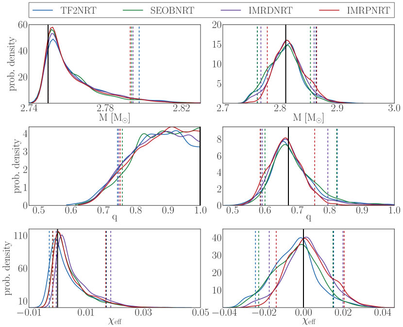
Figure 2: Posterior PDFs of total mass (top row), mass ratio (middle row) and the effective spin parameter $\chi_{\mathrm{eff}}$ (bottom row) for the 4 PP models, the tidal phasing being given for all by the NRTidal model. The sources injected are an equal-mass injection (left panel) and an unequal-mass injection (right panel). The vertical dashed lines mark the 5% and 95% quantiles, enclosing a 90% credible interval. Note that for the equal mass case the lower bound of the 90% confidence interval is indistinguishable from the injected value (black vertical line).

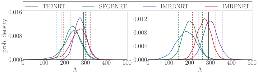
Figure 3: Recovery of tidal deformability $\tilde{\Lambda}$ from a simulation of a non-spinning equal-mass binary of component masses 1.375 ${\rm M_{\odot}}$ each and a tidal deformability $\tilde{\Lambda}$ of 292 (left figure) and the same for an unequal-mass source of 1.68 + 1.13 ${\rm M_{\odot}}$ and $\tilde{\Lambda}$ of 292 (right figure). The simulated waveform model is IMRPNRT, the tidal descriptions in the simulated and recovery models are the NRTidal model. The recovery models are IMRPNRT (in red), TF2NRT (in blue), IMRDNRT (in purple) and SEOBNRT (in green). The vertical lines correspond to the 5% and 95% quantiles respectively. The injected values are shown as a vertical black line.

Within this work, we compare three different types of aligned-spinning PP baseline models: the analytical TF2 model, the EOB-based SEOB model, and the phenomenological IMRD approximant. The IMRP baseline is obtained by ‘twisting up’ IMRD. As we inject a non-spinning IMRPNRT signal, we shall be referring in the following to the IMRDNRT waveform, which in the non-spinning limit has the same PP baseline.

The phase differences between the waveform models with respect to the IMRD approximant are shown in Fig. 1 on a linear scale (top panel) and logarithmic scale (bottom panel). The left column refers to the equal-mass, the right column to the unequal-mass setup. To compute the phase difference, we align the individual waveforms at a frequency of $f_{0}=23~{}\rm Hz$ for the equal-mass setup, whereas for the unequal-mass setup, we align the individual waveforms at a frequency $f_{0}=28~{}\rm Hz$ as the oscillatory behavior for SEOB(caused by the Fourier transformation and ROM computation) makes the alignment non-trivial. During the alignment procedure, we set the phase $\psi(f_{0})$ and the first derivative $\partial_{f}\psi|_{f_{0}}$ of the waveform approximants to be equal at $f_{0}$.

We find that the phase differences between TF2/SEOB and IMRD are comparable and of the order of about 2-3 radians for the equal-mass case and about 1 radian larger for the unequal mass case. Interestingly, both the phase differences are negative. This indicates that IMRD is less attractive than the two other approximants. Consequently, one could expect that the more attractive point particle models TF2 and SEOB will predict smaller tidal phase corrections than the IMRD model under the assumption that all the other recovered parameters are identical.

For completeness, and also because of difficulties in aligning the SEOB waveform due to oscillatory behavior of the waveform’s phase at low frequencies, we tested an alignment for $f_{0}=2048~{}\rm Hz$, i.e., the end of the considered frequency window. For this case the dephasing between SEOB and IMRD is less than 1 radian and for TF2 and IMRD is about 5 radians, with slightly larger phase difference for the unequal mass setup. This clearly shows that the SEOB and IMRD approximant are more similar during the late inspiral, close to the moment of merger, than TF2 and SEOB.

III.2 Estimating non-tidal parameters

We study the impact of the PP baseline on the estimation of the intrinsic parameters by adding the NRTidal contribution to the 4 PP baselines described in Tab. 1. Figure 2 shows the recovery of the intrinsic parameters (from top to bottom): total mass $M$, the mass ratio $q$, and the effective spin $\chi_{\mathrm{eff}}$. The results are presented for both the equal-mass source (left panel) and the unequal-mass source (right panel), cf. Tab. 2. We find for both cases that all values are recovered in a way that the injected value (solid black line) lies within the 90% credible interval (dashed lines). Considering the recovery of the total mass, one finds that the equal mass setup shows more accurate recovery visible by the smaller credible interval; note the different abscissa ranges of the top panels. However, for the equal-mass source, the injected total mass lies at the edge of the 5% quantile. This is because of the condition of $M_{A}\geq M_{B}$ imposed during sampling and is further evidenced in the upper bound on the posterior PDF for $q$ for the same source. For the unequal mass system, we find that the total mass is well constrained, being $M=2.81^{2.86}_{2.77}$ for the IMRDNRT recovery, with the estimates from the other approximants being almost identical.

Considering the recovery of the mass-ratio $q$, for the equal-mass case, we report the lower bound at 90% confidence and show similar recovery for the different waveform approximants. For the unequal-mass case however, the recovered value peaks around the injected one, and is also consistent among all the models. This emphasizes the small systematic bias with respect to different waveform approximants.

The recovery of the effective aligned-spin parameter $\chi_{\mathrm{eff}}$ is similar for all the baseline models, with the injected value lying well within the 5% and 95% quantiles in the unequal-mass simulation.

III.3 Estimating tidal parameters

Figure 3 shows the recovery of the tidal deformability parameter. For the equal-mass case, we note that the injected value of $\tilde{\Lambda}$ (shown by the black vertical line) is always contained within the 5% and 95% quantiles of the posterior distribution. The recovery with the IMRDNRT model shows the smallest offset and spread around the injected value. This is caused by the fewer number of parameters of the IMRDNRT approximant compared to the IMRPNRT model, which is precessing. This observation supports the use of spin-aligned models for the extraction of parameters in addition to precessing models. The SEOBNRT and TF2NRT model differ from the injected value because of the different underlying spin-aligned baseline family. As suggested by the phasing in Fig. 1, we find that SEOBNRT and TF2NRT predict smaller tidal deformability due to the slightly more attractive PP baseline. For the unequal-mass binary, the injected value is contained within the 5% and 95% quantiles only when the recovery PP baseline is the Phenom model. Although the other instrinsic parameters show very similar results from recovering with different PP baseline models, we note that the recovery of the $\tilde{\Lambda}$ parameter differs between waveform models with different PP baselines even when the tidal phasing is unchanged.

 

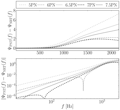
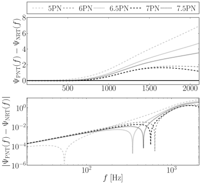
Figure 4: Figure showing the difference between the tidal phasing terms from PN approximation and the NRTidal description for an equal-mass BNS source (left figure) and for an unequal-mass BNS source (right figure), cf. Tab. 2. The top panel shows the differences starting from the leading order PN-tidal phase at 5PN through the highest known order at 7.5PN. The bottom panels show the absolute difference of the phasing terms.

IV Imprint of the tidal description

IV.1 Theoretical modeling

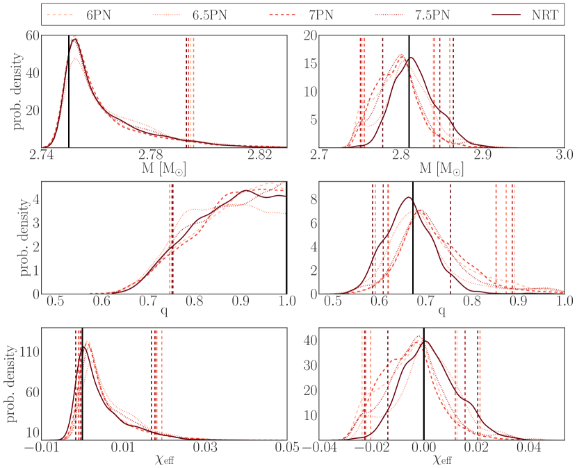
Figure 5: Posterior PDFs of total mass (top row), mass ratio (middle row) and the effective spin parameter $\chi_{\mathrm{eff}}$ (bottom row) for the IMRP PP model and the tidal phasing given by the PN description starting from 6PN through 7.5PN and the phasing described by the NRTidal model. The sources injected are an equal-mass binary (left panel) and an unequal-mass binary (right panel), cf. Tab. 2 The injected values are shown by black, vertical lines whereas the dashed lines show the 90% credible interval.

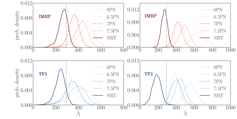
Figure 6: Posterior probability distributions showing estimates of $\tilde{\Lambda}$ from a simulation of of an equal-mass BNS source with IMRPNRT (left figure) and an unequal-mass BNS source with IMRPNRT (right figure). The point-particle baseline recovery waveform models are IMRP (top panel) and TF2 (bottom panel). The tidal phasing in each model is varied from 6PN through 7.5PN and the NRTidal description. The gray dashed line shows the injected value.

Recovery model		Equal-mass case ($\tilde{\Lambda}=292$)		Unequal-mass case ($\tilde{\Lambda}=292$)
Baseline	Tidal phasing	Estimate of $\tilde{\Lambda}$	Systematic bias (stacc)	Estimate of $\tilde{\Lambda}$	Systematic bias (stacc)
TF2	6PN	$350.3_{215.8}^{445.1}$	87.8	$388.4_{310.7}^{465.4}$	107.0
	6.5PN	$425.7_{245.7}^{564.6}$	158.3	$554.1_{452.7}^{669}$	272.6
	7PN	$343.7_{222.2}^{441}$	82.1	$398.6_{310.7}^{489.8}$	120.7
	7.5PN	$388.8_{225.7}^{500.8}$	122.2	$446.7_{357.5}^{543.7}$	165.6
	NRTidal	$241.3_{159.2}^{303.3}$	70.4	$184.6_{106.6}^{260.6}$	117.5
IMRP	6PN	$375.4_{281.8}^{448.3}$	95.2	$437.5_{357.5}^{514.9}$	152.7
	6.5PN	$472.4_{333.2}^{578.8}$	189.3	$644.1_{508.0}^{782.9}$	362.8
	7PN	$360.9_{278.2}^{432.4}$	82.6	$415.9_{331.8}^{498.7}$	133.9
	7.5PN	$428.0_{308.2}^{512.9}$	144.2	$493.1_{388.3}^{584.8}$	207.5
	NRTidal	$268.9_{193.6}^{326}$	48.8	$270.0_{214.8}^{322.9}$	39.9
IMRD	NRTidal	$274.7_{230.2}^{322.1}$	32.8	$299.8_{244.5}^{359.8}$	36.3
SEOB	NRTidal	$239.9_{183.2}^{300.9}$	62.5	$201.7_{147.8}^{261.7}$	95.8

Table 3: Results from parameter estimation study with simulation of IMRPNRT for an equal-mass and unequal-mass source.

As given explicitly in Eq. (4) there exist analytical (although incomplete) PN knowledge up 7.5PN oder. To understand the imprint of the employed PN order, we present the phase difference between the different PN-tidal phase contributions with respect to the NRTidal model, Eq. (8), in Fig. 4. We employ the NRTidal model as our benchmark since it has been shown to reliably agree with NR waveforms Dietrich et al. (2017, 2018a) as well as with hybrid TEOBResumS Bernuzzi et al. (2015); Nagar et al. (2018)/NR hybrids Dietrich et al. (2018b). Nevertheless, we stress that also the NRTidal phasing potentially overestimates tidal effects with respect to TEOBResumS/NR-hybrids Dietrich et al. (2018b); Dudi et al. (2018).

The PN-based phasing terms are considered starting from the single leading-order term at 5PN to the higher order terms, which also include the preceding orders. The absolute value of the difference of these terms is plotted in the bottom panel of the figure on a double logarithmic scale. We note that the terms at 7PN and 6PN are closer to the NRTidal description than the half PN orders at 6.5PN and 7.5PN. This is related to the half-PN orders being repulsive. The plot refers to our fiducial equal-mass (left) and unequal mass (right) BNS, cf. Tab. 2.

IV.2 Estimating non-tidal parameters

Figure 5 shows the results from parameter estimation of the equal-mass setup (left panel) and the unequal-mass setup (right panel). We recover the parameters with IMRPNRT and IMRPPNT (with the tidal phasing varying from 6PN through 7.5PN orders). We find overall that for the equal mass configuration the estimation of the total mass, mass ratio, and effective spin is almost unaffected by the choice of the tidal contribution. A similar statement is true when one uses TF2 as a PP baseline. Although the recovered values differ more for the unequal-mass configuration, the injected values are contained within the 5% and 95% quantiles for each approximant. However, the most notable difference is that the PN-tidal approximants predict mass ratios (credible intervals) larger than the NRTidal description.

IV.3 Estimating tidal parameters

Figure 6 shows the results considering the parameter estimation of the tidal deformability for the equal-mass (left panel) and unequal-mass (right panel) binary sources. We recover the parameters with the IMRPNRT and IMRPPNT models (red) and with the TF2NRT and TF2PNT (blue). It is expected that the recovery with IMRPNRT would be exact, except limitations from statistical uncertainties. The simulated signal however has a very high SNR, $\sim\ 87$, and we therefore ignore presence of statistical biases in our study.

For the equal-mass injection in Fig. 6, as seen also from the tidal phasing from Fig. 4, we find that the recoveries with the 6PN and 7PN orders in IMRPPNT lie closer to the injected IMRPNRT approximant than the half-PN orders. We observe a similar trend in the TF2 recoveries, albeit with a constant shift due to the difference in the PP baseline models between the injection and recovery. Table 3 quotes the median values of $\tilde{\Lambda}$ posterior PDFs and the 5% and 95% quantiles. We note that the injected value is always within this interval.

In case of the unequal-mass injection, the estimates deteriorate and the recovery with TF2 and SEOB lead to an incorrect measurement. Table 3 also summarizes the inferred values of $\tilde{\Lambda}$ for the unequal-mass simulation and we find that the injected value lies within the 5% and 95% quantiles only with the recovery with the IMRPNRT and IMRDNRT models. We quantify the systematic bias with the standard accuracy statistic (stacc) defined as

$$S=\sqrt{\frac{1}{N}\sum_{i=1}^{N}(x_{i}-x_{\mathrm{inj}})^{2}},$$ (18)

where $N$ is the number of samples, $x_{i}$ is the $i^{th}$ posterior sample and $x_{\mathrm{inj}}$ is the injected value of the parameter $x$, here $\tilde{\Lambda}$. The lowest values of $S$ are indeed obtained for the recovery model IMRDNRT and is followed by IMRPNRT. When the simulated source is an unequal-mass binary, the statistic is steadily higher than for the equal-mass configuration, again showing the general deterioration of estimation of the tidal deformability parameter.

V Conclusion

We studied possible systematic biases caused by the choice of the waveform approximants during the recovery of the source parameters from future detections. The studied cases had an SNR of $\sim 87$. Expecting the design sensitivity of Advanced LIGO and Virgo to be about three times better than the current sensitivity, this SNR would correspond approximately to that of a GW170817-like system at design sensitivity.

We find that for such scenarios the existing waveform model approximants would be sufficient to extract non-tidal parameters as masses, mass ratios, and spins. On the contrary, the measurement of the tidal deformability can be significantly biased up to a point where the injected value is not contained within the 90% credible interval.

In particular, the large systematic errors for unequal mass systems, might lead to misclassification of BNS, BBH, and neutron star-black hole systems. Thus, better waveform models with improved tidal descriptions are imperative for characterizing unequal-mass BNS and/or NSBH systems in the advanced detector era. These improvements have to include (i) a calibration of the NRTidal model to unequal mass binaries; (ii) an incorporation of analytical knowledge beyond 6PN knowledge in the NRTidal model.

In a future publication, we will address the issue of possible systematics arising from the presence of spins and precession in the simulated sources and the influence of missing spin-tides coupling in the existing waveform approximants.