UMTG–297

The spin-$s$ homogeneous central spin model:
exact spectrum and dynamics
Rafael I. Nepomechie and Xi-Wen Guan $\!{}^{,}$ $\!{}^{,}$

We consider the problem of a central spin with arbitrary spin $s$ that interacts pairwise and uniformly with a bath of $N$ spins with $s=1/2$. We present two approaches for determining the exact spectrum of this model, one based on properties of $SU(2)$, and the other based on integrability. We also analyze the exact time evolution of a spin coherent state, and compute the time evolution of various quantities of physical interest, including the entanglement entropy, spin polarization and Loschmidt echo.

1 Introduction

The (spin-$\frac{1}{2})$ central spin model is a simple quantum mechanical model of a central spin $\vec{s}_{0}$ interacting pairwise with a “bath” of $N$ surrounding spins $\vec{s}_{1},\ldots,\vec{s}_{N}$, with the Hamiltonian

$$H^{(\frac{1}{2})}_{\rm{inhom}}=Bs^{z}_{0}+2\sum_{j=1}^{N}A_{j}\vec{s}_{0}\cdot\vec{s}_{j}\,,$$ (1.1)

where $B$ and $A_{j}$ are real constants. This is a special case of the Richardson-Gaudin model, which was formulated long ago [1, 2, 3, 4]. Nevertheless, this model is the focus of renewed attention due to its interesting new applications, such as quantum dots (see e.g. [5, 6, 7, 8, 9, 10, 11, 12] and references therein). The homogeneous case $A_{j}=A$ is simple enough to allow for analytical analysis of spin dynamics, yet exhibits rich phenomena such as quantum collapse and revival [13, 14, 15]. Moreover, it can be mapped [13, 15] to a generalization of the Jaynes-Cummings model [16, 17, 18] of quantum nonlinear optics.

We consider here a generalization of this model, whereby the central spin $\vec{S}_{0}$ has spin $s$. We focus primarily on the homogeneous case

$$H^{(s)}=BS^{z}_{0}+2A\sum_{j=1}^{N}\vec{S}_{0}\cdot\vec{s}_{j}\,,\qquad s=\tfrac{1}{2},1,\ldots\,.$$ (1.2)

This model, which to our knowledge has not been considered before, has the potential to be realized experimentally, and exhibits interesting quantum dynamics. It can also be mapped to a generalization of the Tavis-Cummings model [19, 17] of quantum nonlinear optics, see e.g. [20, 21, 22, 18] for recent work.

The outline of this paper is as follows. In Section 2, we discuss two approaches for determining the exact spectrum of the model, one based on properties of $SU(2)$, and the other based on integrability. We also briefly describe the connection with the Tavis-Cummings model. In Section 3, we analyze the exact time evolution of a spin coherent state. Readers who are primarily interested in spin dynamics can jump directly to this section, as it is largely independent of the previous one. We conclude with a brief summary. Appendix A contains the derivation of a key step in our analysis of spin dynamics, while Appendix B contains the derivation of some useful identities.

2 Exact spectrum

We briefly discuss here two approaches for determining the spectrum of the spin-$s$ homogeneous central spin model (1.2). The first approach exploits the partial $SU(2)$ symmetry of the problem, and in principle can give the entire spectrum. The second approach exploits the integrability of the model; however, it remains to be understood whether the solution obtained in this way can give the full spectrum.

2.1 $SU(2)$-based approach

The Hamiltonian (1.2) can evidently be rewritten as

$$H^{(s)}=BS^{z}_{0}+2A\vec{S}_{0}\cdot\vec{J}\,,$$ (2.1)

where

$$\vec{J}=\sum_{j=1}^{N}\vec{s}_{j}$$ (2.2)

is the total spin of the bath. This Hamiltonian clearly has the properties

$$\left[H^{(s)}\,,\vec{J}^{2}\right]=0\,,\qquad\left[H^{(s)}\,,\vec{S}_{0}^{2}\right]=0\,,$$ (2.3)

as well as the $U(1)$ symmetry

$$\left[H^{(s)}\,,{\cal S}^{z}\right]=0\,,\qquad{\cal S}^{z}=J^{z}+S^{z}_{0}\,,$$ (2.4)

but (for $B\neq 0$) does not have the full $SU(2)$ symmetry. In view of (2.3) and (2.4), we look for simultaneous eigenstates of $H$, ${\cal S}^{z}$, $\vec{S}_{0}^{2}$, $\vec{J}^{2}$,

$$H^{(s)}|E,m,s,j\rangle =E|E,m,s,j\rangle\,,$$

$${\cal S}^{z}|E,m,s,j\rangle =m|E,m,s,j\rangle\,,$$

$$\vec{S}_{0}^{2}|E,m,s,j\rangle =s(s+1)|E,m,s,j\rangle\,,$$

$$\vec{J}^{2}|E,m,s,j\rangle =j(j+1)|E,m,s,j\rangle\,.$$ (2.5)

We can expand these states in the standard orthonormal spin basis as follows

$$|E,m,s,j\rangle=\sum_{m_{s}=-s}^{s}\sum_{m_{j}=-j}^{j}w_{m_{s},m_{j}}^{(E,m,s,j)}\delta_{m_{s}+m_{j},m}|s,m_{s}\rangle\otimes|j,m_{j}\rangle\,,$$ (2.6)

where the coefficients $w_{m_{s},m_{j}}^{(E,m,s,j)}$ are still to be determined. Note that the allowed values of $j$ (spin of the bath) are

$$j=\left\{\begin{array}[]{ll}0,1,\ldots,\frac{N}{2}&\mbox{ for }N=\mbox{ even }\\ \\ \frac{1}{2},\frac{3}{2},\ldots,\frac{N}{2}&\mbox{ for }N=\mbox{ odd }\end{array}\right.\,,$$ (2.7)

while the allowed values of $m$ are given by

$$-j-s\leq m\leq j+s\,.$$ (2.8)

We now act on (2.6) with the Hamiltonian (2.1) in the form

$$H^{(s)}=BS^{z}_{0}+A\left(S^{+}_{0}J^{-}+S^{-}_{0}J^{+}+2S^{z}_{0}J^{z}\right)\,,$$ (2.9)

where $S^{\pm}=S^{x}\pm iS^{y}$ (and similarly for $J^{\pm}$). Using the familiar $SU(2)$ raising/lowering formulas

$$S^{\pm}|s,m\rangle=\sqrt{(s\mp m)(s\pm m+1)}|s,m\pm 1\rangle\,,$$ (2.10)

we obtain

$$H^{(s)}|E,m,s,j\rangle =\sideset{}{{}^{\prime}}{\sum}_{m_{s},m_{j}}w_{m_{s},m_{j}}^{(E,m,s,j)}\Bigg{\{}\mu_{m_{s},m_{j}}|s,m_{s}\rangle\otimes|j,m_{j}\rangle$$

$$+\nu_{m_{s}+1,m_{j}-1}^{(s,j)}|s,m_{s}+1\rangle\otimes|j,m_{j}-1\rangle+\nu_{-m_{s}+1,-m_{j}-1}^{(s,j)}|s,m_{s}-1\rangle\otimes|j,m_{j}+1\rangle\Bigg{\}}\,,$$ (2.11)

where the summation is constrained by $m_{s}+m_{j}=m$, and the coefficients are defined by

$$\mu_{m_{s},m_{j}} =B\,m_{s}+2A\,m_{s}\,m_{j}\,,$$

$$\nu_{m_{s},m_{j}}^{(s,j)} =A\sqrt{(s-m_{s}+1)(s+m_{s})(j+m_{j}+1)(j-m_{j})}\,.$$ (2.12)

Finally, using the orthonormality of the basis, we arrive at an eigenvalue relation for the energy $E$ and the corresponding coefficients $w_{m_{s},m_{j}}^{(E,m,s,j)}$,

$$\mu_{m_{s},m_{j}}\,w_{m_{s},m_{j}}^{(E,m,s,j)}+\nu_{m_{s},m_{j}}^{(s,j)}\,w_{m_{s}-1,m_{j}+1}^{(E,m,s,j)}+\nu_{-m_{s},-m_{j}}^{(s,j)}\,w_{m_{s}+1,m_{j}-1}^{(E,m,s,j)}=E\,w_{m_{s},m_{j}}^{(E,m,s,j)}\,,$$

$$m_{s}=-s,\ldots,s\,,\qquad m_{j}=-j,\ldots,j\,,\qquad m_{s}+m_{j}=m\,.$$ (2.13)

Letting $d(m,s,j)$ denote the number of allowed values of $(m_{s},m_{j})$ satisfying $m_{s}+m_{j}=m$, we see that (2.13) entails diagonalizing a $d(m,s,j)\times d(m,s,j)$ matrix.

The eigenvalue relation (2.13) for the energy is the main result of this subsection. Given values of $j$ and $m$ (constrained by (2.7) and (2.8), respectively), the eigenvalue problem (2.13) can in principle be solved for the corresponding energies. The advantage of this approach over brute-force diagonalization of the full Hamiltonian (2.1) is that the matrices to be diagonalized are much smaller. Of course, as the bath size $N$ becomes large, the number of possible values for $j$ and $m$ also becomes large.

As a simple example, we present in Table 1 the energies that are computed in this way for the case $s=1\,,N=2$. (The final two columns of the table are explained in the following subsection.)

$j$	$m$	$E$	$M$	$\{v_{a}\}$
1	2	1.5	0	-
1	1	-0.780776	1	-0.438447
1	1	1.28078	1	-4.56155
1	0	-2.14854	2	-0.351465 $\pm 0.262932i$
1	0	-0.893401	2	-2.71954, -0.493659
1	0	1.04194	2	-3.54194 $\pm 1.70866i$
1	-1	-1.28078	3	-0.612504, -1.41297 $\pm 0.681796i$
1	-1	0.780776	3	-3.16744, -2.19705 $\pm 2.46224i$
1	-2	0.5	4	-2.26566 $\pm 0.850941i$, -0.734342 $\pm 2.43893i$
0	1	0.5
0	0	0
0	-1	- 0.5

Table 1: The energies ($E$) and Bethe roots $\{v_{1},\ldots,v_{M}\}$ for the Hamiltonian (1.2) with $s=1,N=2,A=B=0.5$. The total number of levels is $(2s+1)2^{N}=12$.

2.2 Bethe ansatz approach

The spin-$s$ central spin model (1.2) is integrable, as is the original model with $s=\frac{1}{2}$. We present here its Bethe ansatz solution, but only sketch the derivation, since it is similar to the one for the spin-$\frac{1}{2}$ case, see e.g. [23, 24, 25]. For pedagogical reasons, we in fact work for the inhomogeneous model (which is also integrable), and consider the homogeneous limit only at the end.

2.2.1 Inhomogeneous case

Our starting point is the $SU(2)$-invariant $(\frac{1}{2},s)$ R-matrix on ${\cal C}^{2}\otimes{\cal C}^{2s+1}$ (see, e.g. [26]),

$$R^{(\frac{1}{2},s)}(u)=\frac{1}{u+(s+\frac{1}{2})\eta}\left((u+\frac{\eta}{2})\mathbb{I}+2\eta\vec{s}\overset{\cdot}{\otimes}\vec{S}\right)\,,\qquad s=\tfrac{1}{2}\,,1\,,\ldots\,,$$ (2.14)

where (as above) $\vec{s}$ and $\vec{S}$ denote the spin operators for spin-$\frac{1}{2}$ and spin-$s$, respectively. This R-matrix is a solution of the Yang-Baxter equation on ${\cal C}^{2}\otimes{\cal C}^{2}\otimes{\cal C}^{2s+1}$

$$R^{(\frac{1}{2},\frac{1}{2})}_{12}(u-v)\,R^{(\frac{1}{2},s)}_{13}(u)\,R^{(\frac{1}{2},s)}_{23}(v)=R^{(\frac{1}{2},s)}_{23}(v)\,R^{(\frac{1}{2},s)}_{13}(u)\,R^{(\frac{1}{2},\frac{1}{2})}_{12}(u-v)\,.$$ (2.15)

We introduce the following monodromy matrix

$$T_{a}(u)=G_{a}\,R^{(\frac{1}{2},\frac{1}{2})}_{aN}(u-\epsilon_{N})\,\ldots R^{(\frac{1}{2},\frac{1}{2})}_{a1}(u-\epsilon_{1})\,R^{(\frac{1}{2},s)}_{a0}(u-\epsilon_{0})\,,\qquad G=e^{\eta sB\sigma^{z}}\,,$$ (2.16)

where the “auxiliary” space (denoted by $a$) has dimension 2, and there are $N+1$ “quantum” spaces (denoted by $0,1,\ldots,N$): the $0^{th}$ quantum space (corresponding to the central spin) has dimension $2s+1$, while all the others (corresponding to the bath) have dimension 2. Notice that there are arbitrary inhomogeneities $\epsilon_{0},\ldots,\epsilon_{N}$ associated with each of the quantum spaces. Finally, note that there is a diagonal twist, encoded by the matrix $G$, which is responsible for breaking $SU(2)$ down to $U(1)$.

The transfer matrix $t(u)$, obtained by tracing the monodromy matrix over the auxiliary space

$$t(u)=\mathop{\rm tr}\nolimits_{a}T_{a}(u)\,,$$ (2.17)

satisfies the important commutativity property

$$\left[t(u)\,,t(v)\right]=0$$ (2.18)

owing to the Yang-Baxter equation (2.15).

The basic idea, following e.g. [23, 24, 25], is to evaluate the transfer matrix at $u=\epsilon_{0}$ and expand in terms of $\eta$. We find that the inhomogeneous spin-$s$ Hamiltonian

$$H^{(s)}_{\rm{inhom}}=BS^{z}_{0}+\frac{1}{s}\sum_{j=1}^{N}\frac{1}{\epsilon_{0}-\epsilon_{j}}\vec{S}_{0}\cdot\vec{s}_{j}$$ (2.19)

can indeed be obtained in this way

$$H^{(s)}_{\rm{inhom}}=\frac{(2s+1)}{4s}\frac{d}{d\eta}t(\epsilon_{0})\Big{|}_{\eta=0}+\frac{1}{4s}\sum_{j=1}^{N}\frac{1}{\epsilon_{0}-\epsilon_{j}}\mathbb{I}\,.$$ (2.20)

Using algebraic Bethe ansatz (ABA), we find that the eigenvalues of the transfer matrix (2.17) are given by

$$\Lambda(u)=e^{\eta sB}\prod_{a=1}^{M}\frac{u-v_{a}-\eta}{u-v_{a}}+e^{-\eta sB}\left(\frac{u-\epsilon_{0}+(\frac{1}{2}-s)\eta}{u-\epsilon_{0}+(\frac{1}{2}+s)\eta}\right)\prod_{j=1}^{N}\frac{u-\epsilon_{j}}{u-\epsilon_{j}+\eta}\prod_{a=1}^{M}\frac{u-v_{a}+\eta}{u-v_{a}}\,,$$ (2.21)

where $\{v_{1}\,,\ldots\,,v_{M}\}$ are solutions of the Bethe equations

$$\left(\frac{v_{a}-\epsilon_{0}+(\frac{1}{2}-s)\eta}{v_{a}-\epsilon_{0}+(\frac{1}{2}+s)\eta}\right)\prod_{j=1}^{N}\frac{v_{a}-\epsilon_{j}}{v_{a}-\epsilon_{j}+\eta}=e^{2\eta sB}\prod_{b=1,b\neq a}^{M}\frac{v_{a}-v_{b}-\eta}{v_{a}-v_{b}+\eta}\,,\quad a=1,\ldots,M\,.$$ (2.22)

It follows from (2.20) that the eigenvalues of $H^{(s)}_{\rm{inhom}}$ are given by

$$E_{\rm{inhom}} =\frac{(2s+1)}{4s}\frac{d}{d\eta}\Lambda(\epsilon_{0})\Big{|}_{\eta=0}+\frac{1}{4s}\sum_{j=1}^{N}\frac{1}{\epsilon_{0}-\epsilon_{j}}$$

$$=sB+\frac{1}{2}\sum_{j=1}^{N}\frac{1}{\epsilon_{0}-\epsilon_{j}}+\sum_{a=1}^{M}\frac{1}{v_{a}-\epsilon_{0}}\,.$$ (2.23)

Moreover, expanding the Bethe equations (2.22) in $\eta$, we arrive at the Bethe equations for the inhomogeneous spin-$s$ central spin model

$$-2sB-\frac{2s}{v_{a}-\epsilon_{0}}-\sum_{j=1}^{N}\frac{1}{v_{a}-\epsilon_{j}}+2\sum_{b=1,b\neq a}^{M}\frac{1}{v_{a}-v_{b}}=0\,,\quad a=1,\ldots,M\,.$$ (2.24)

The allowed values of $M$ can be deduced from the formula for the ${\cal S}^{z}$ eigenvalues

$$m=\frac{N}{2}+s-M$$ (2.25)

which also follows from the ABA, together with the ranges (2.7) and (2.8). We conclude that the number of Bethe roots can be

$$M=0,1,\ldots,N+2s\,.$$ (2.26)

The energy formula (2.23) and the corresponding Bethe equations (2.24) constitute our main results for the inhomogeneous spin-$s$ central spin model (2.19). For $s=\frac{1}{2}$, the well-known results are recovered. For distinct values of the inhomogeneities ($\epsilon_{j}\neq\epsilon_{k}$ for $j\neq k$) and $B\neq 0$, the spectrum is nondegenerate, and the Bethe ansatz solution appears to be complete. (We have checked this numerically for small values of $s$ and $N$; a proof for the case $s=\frac{1}{2}$ can be found in [27].) We conjecture that the number of solutions of these Bethe equations for given values of $s,N,M$ is given by

$${\cal N}(s,N,M)=\sum_{k=0}^{\lfloor s\rfloor}(-1)^{k}{2s-k\choose k}{N+2s-2k\choose m-k}\,.$$ (2.27)

We have also checked this result numerically for small values of $s$ and $N$, and one can verify that indeed

$$\sum_{M=0}^{N+2s}{\cal N}(s,N,M)=(2s+1)2^{N}\,,$$ (2.28)

thereby accounting for all the levels of the system.

2.2.2 Homogeneous case

Let us finally return to the homogeneous Hamiltonian (1.2). Comparing with the inhomogeneous one (2.19), we see that the homogeneous case corresponds to setting

$$\epsilon_{1}=\ldots=\epsilon_{N}\equiv\epsilon\,,\qquad A=\frac{1}{2s(\epsilon_{0}-\epsilon)}\,.$$ (2.29)

For these values of parameters, the formulas for the energy (2.23) and the Bethe equations (2.24) reduce to

$$E=s(B+NA)+\sum_{a=1}^{M}\frac{1}{v_{a}}$$ (2.30)

and

$$-2sB-\frac{2s}{v_{a}}-\frac{N}{v_{a}+\frac{1}{2sA}}+2\sum_{b=1,b\neq a}^{M}\frac{1}{v_{a}-v_{b}}=0\,,\quad a=1,\ldots,M\,,$$ (2.31)

respectively, after performing a shift $v_{a}\mapsto v_{a}+\epsilon_{0}$ of all the Bethe roots. Eqs. (2.30) and (2.31) constitute our main results for the Bethe ansatz solution of the homogeneous model.

A simple example with $s=1$ and $N=2$ is presented in Table 1. Note that all the levels with $j=\frac{N}{2}$ are accounted for, but not those with $j<\frac{N}{2}$. This appears to be a general feature of the Bethe ansatz solution for the homogeneous model. Our preliminary investigations indicate that this difficulty (which is present already for the spin-$\frac{1}{2}$ case) is due to the necessity of correctly taking into account so-called singular solutions (e.g., $v=0$). We hope to investigate this matter further in the future.

A nice feature of the Bethe equations (2.31) is that numerical solutions can be readily found even for relatively large values of $N$ and $M$. The trick (see e.g. [29, 30, 31, 32] begins with the observation that the q-polynomial

$$q(u)=\prod_{a=1}^{M}(u-v_{a})=u^{M}+O(u^{M-1})$$ (2.32)

satisfies

$$\frac{q^{\prime\prime}(v_{a})}{q^{\prime}(v_{a})}=2\sum_{b=1,b\neq a}^{M}\frac{1}{v_{a}-v_{b}}\,.$$ (2.33)

The Bethe equations (2.31) can therefore be rewritten in the form

$$P(v_{a})=0\,,\qquad a=1,\ldots,M\,,$$ (2.34)

where

$$P(u)=u(u+\frac{1}{2sA})q^{\prime\prime}(u)-2sBu(u+\frac{1}{2sA})q^{\prime}(u)-2s(u+\frac{1}{2sA})q^{\prime}(u)-Nuq^{\prime}(u)\,.$$ (2.35)

One next observes that $P(u)$ is a polynomial in $u$ of degree $M+1$, which has all $M$ zeros of the polynomial $q(u)$. Therefore, $P(u)/q(u)$ is a polynomial of degree 1, i.e.

$$P(u)=(a+b\,u)\,q(u)\,,$$ (2.36)

where $b=-2sBM$ follows from the asymptotic behavior $u\rightarrow\infty$. Setting

$$q(u)=\sum_{k=0}^{M}q_{k}u^{k}\,,$$ (2.37)

one can obtain from (2.36) (by setting the coefficients of $u^{0}\,,\ldots\,,u^{M+1}$ equal to zero) a set of $M+2$ equations for the $M+2$ unknowns $a,q_{0},\ldots,q_{M}$, which can be readily solved numerically even for relatively large values of $N$ and $M$; one can then determine the zeros of $q(u)$, which are the sought-after Bethe roots. An example with $N=60,s=1,M=31$ is shown in Figure 1.

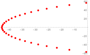
Figure 1: A set of solutions of the Bethe equations (2.31) plotted in the complex $v$ plane for $N=60,s=1,M=31,A=B=0.5$, with corresponding energy $E=30.004$.

2.3 Connection with the Tavis-Cummings model

We briefly note here a mapping of the spin-$s$ homogeneous central spin model to the Tavis-Cummings model [19, 17]. This mapping relies, as in the spin-$\frac{1}{2}$ case [13, 15], on the Holstein-Primakoff transformation [33]:

$$J^{+}=\sqrt{N}a^{\dagger}\sqrt{1-\frac{a^{\dagger}a}{N}}\,,\qquad J^{-}=\left(J^{+}\right)^{\dagger}=\sqrt{N}\sqrt{1-\frac{a^{\dagger}a}{N}}\,a\,,\qquad J^{z}=a^{\dagger}a-\frac{N}{2}\,,$$ (2.38)

where $\left[a\,,a^{\dagger}\right]=1$. Indeed, let us now consider an anisotropic generalization of the Hamiltonian (2.9),

$$H^{(s)}=BS^{z}_{0}+A\left(S^{+}_{0}J^{-}+S^{-}_{0}J^{+}\right)+2\Delta\,S^{z}_{0}J^{z}\,,$$ (2.39)

where $\Delta$ is the anisotropy parameter. Applying the transformation (2.38), and letting $N\rightarrow\infty$, we obtain

$$H^{(s)}\sim(B-\Delta N)S^{z}_{0}+A\sqrt{N}\left(S^{+}_{0}\,a+S^{-}_{0}\,a^{\dagger}\right)+2\Delta S^{z}_{0}\,a^{\dagger}a\,.$$ (2.40)

The case $\Delta=0$ reduces to the Tavis-Cummings model, while the isotropic case $\Delta=A$ corresponds to a generalization of the Tavis-Cummings model.

3 Exact dynamics

We turn now to the question of how states evolve in time for the spin-$s$ homogeneous central spin model (1.2), (2.1). For a generic initial state, this problem appears to pose a formidable challenge, even for a model as simple as this one. However, if the initial state is an eigenstate of $\vec{S}_{0}^{2}$ and $\vec{J}^{2}$, then the symmetries (2.3) and (2.4) significantly constrain the possible intermediate states, and the problem becomes tractable yet nevertheless remains nontrivial.

3.1 Time evolution of a spin coherent state

Following [13, 14], we assume that the bath is initially in a so-called spin coherent state [34, 35]

$$|\theta\rangle=\bigotimes_{j=1}^{N}\left[\cos(\tfrac{\theta}{2})|\tfrac{1}{2},\tfrac{1}{2}\rangle_{j}+\sin(\tfrac{\theta}{2})|\tfrac{1}{2},-\tfrac{1}{2}\rangle_{j}\right]\,,$$ (3.1)

which indeed is an eigenstate of $\vec{J}^{2}$ with $j=\frac{N}{2}$. Moreover, we assume that the central spin is initially “up”, i.e. in the state $|s,s\rangle_{0}$. Thus, the initial state of the system is

$$|\Psi(0)\rangle=|s,s\rangle\otimes|\theta\rangle\,,$$ (3.2)

and our task is to determine its time evolution

$$|\Psi(t)\rangle=e^{-iH^{(s)}t}|\Psi(0)\rangle\,.$$ (3.3)

Expressing the spin coherent state in terms of so-called Dicke states as in [13, 15]

$$|\theta\rangle=\sum_{n=0}^{N}\sqrt{{N\choose n}}\cos^{N-n}(\tfrac{\theta}{2})\sin^{n}(\tfrac{\theta}{2})|n\rangle\,,$$ (3.4)

where $|n\rangle\equiv|\frac{N}{2},\frac{N}{2}-n\rangle$, the problem reduces to computing

$$|\Psi(t)\rangle =\sum_{k=0}^{\infty}\frac{1}{k!}(-iH^{(s)}t)^{k}|\Psi(0)\rangle$$

$$=\sum_{n=0}^{N}\sqrt{{N\choose n}}\cos^{N-n}(\tfrac{\theta}{2})\sin^{n}(\tfrac{\theta}{2})\sum_{k=0}^{\infty}\frac{(-it)^{k}}{k!}(H^{(s)})^{k}\left(|s,s\rangle\otimes|n\rangle\right)\,.$$ (3.5)

Due to the $U(1)$ symmetry (2.4), we know that

$$(H^{(s)})^{k}\left(|s,s\rangle\otimes|n\rangle\right)=\sum_{j=0}^{2s}h^{(s,k)}_{j}|s,s-j\rangle\otimes|n-j\rangle\,,$$ (3.6)

where the coefficients $h^{(s,k)}_{j}$ are still unknown. We show in Appendix A that these coefficients are given by

$$h_{j}^{(s,k)}=\sum_{l=0}^{2s}c_{j,l}^{(s)}(n)\,\left(\omega_{l}^{(s)}(n)\right)^{k}\,,\qquad j=0,1,\ldots,2s\,,$$ (3.7)

see (A.15), and we provide a straightforward recipe for numerically computing $c_{j,l}^{(s)}(n)$ and $\omega_{l}^{(s)}(n)$. Substituting the results (3.6) and (3.7) back into (3.5), we obtain

$$|\Psi(t)\rangle =\sum_{n=0}^{N}\sqrt{{N\choose n}}\cos^{N-n}(\tfrac{\theta}{2})\sin^{n}(\tfrac{\theta}{2})\sum_{j=0}^{2s}\sum_{l=0}^{2s}c_{j,l}^{(s)}(n)\,\sum_{k=0}^{\infty}\frac{(-it)^{k}}{k!}\left(\omega_{l}^{(s)}(n)\right)^{k}|s,s-j\rangle\otimes|n-j\rangle$$

$$=\sum_{n=0}^{N}\sqrt{{N\choose n}}\cos^{N-n}(\tfrac{\theta}{2})\sin^{n}(\tfrac{\theta}{2})\sum_{j,l=0}^{2s}c_{j,l}^{(s)}(n)\,e^{-it\omega_{l}^{(s)}(n)}|s,s-j\rangle\otimes|n-j\rangle\,.$$ (3.8)

For given values of $s$, $N$ and $n$, the frequencies $\{\omega_{0}^{(s)}(n)\,,\ldots\,,\omega_{2s}^{(s)}(n)\}$ are the energies in the sector (see Sec. 2.1) with $j=\frac{N}{2}$ and $m=\frac{N}{2}-n+s$, which has (at most) dimension $2s+1$.

An important check on this result is the verification of unitarity $\langle\Psi(t)|\Psi(t)\rangle=1$. Using the orthonormality of the basis and the fact that $c_{j,l}^{(s)}(n)$ and $\omega_{l}^{(s)}(n)$ are real, we obtain

$$\langle\Psi(t)|\Psi(t)\rangle=\sum_{n=0}^{N}{N\choose n}\cos^{2(N-n)}(\tfrac{\theta}{2})\sin^{2n}(\tfrac{\theta}{2})\sum_{j,l,l^{\prime}=0}^{2s}c_{j,l}^{(s)}(n)\,c_{j,l^{\prime}}^{(s)}(n)\,e^{-it\left(\omega_{l}^{(s)}(n)-\omega_{l^{\prime}}^{(s)}(n)\right)}\,.$$ (3.9)

With the help of the identities (see (B.3) and (B.8))

$$\sum_{j=0}^{2s}c_{j,l}^{(s)}(n)\,c_{j,l^{\prime}}^{(s)}(n)=c_{0,l}^{(s)}(n)\,\delta_{l,l^{\prime}}\,,\qquad\sum_{l=0}^{2s}c_{0,l}^{(s)}(n)=1\,,$$ (3.10)

we see that unitarity is indeed preserved.

The result (3.8) is one of the main results of our paper. We emphasize that this is an exact result. Note that the infinite sum over $k$ in (3.5) has been effectuated, leaving only finite sums to be performed (assuming that $N$ and $s$ are finite). For the special case $s=\frac{1}{2}$, the result (3.8) reduces to a corresponding result in [15]. In the remaining part of this section, we use (3.8) to compute the time evolution of various quantities of physical interest.

3.2 Reduced density matrix

The reduced density matrix for the central spin $\rho(t)$ is defined by

$$\rho(t)=\sum_{\alpha}\langle\alpha|\Psi(t)\rangle\langle\Psi(t)|\alpha\rangle\,,$$ (3.11)

where the trace is performed by summing over an orthonormal basis of the bath $({\cal C}^{2})^{\otimes N}$. Making use of the result (3.8) and the fact

$$\sum_{\alpha}\langle\alpha|n-j\rangle\langle n^{\prime}-j^{\prime}|\alpha\rangle=\delta_{n-j,n^{\prime}-j^{\prime}}\,,$$ (3.12)

we obtain the $(2s+1)\times(2s+1)$ matrix

$$\rho(t)=\sum_{j,j^{\prime}=0}^{2s}\rho_{jj^{\prime}}(t)|s-j\rangle\langle s-j^{\prime}|\,,$$ (3.13)

whose matrix elements are given by

$$\rho_{jj^{\prime}}(t) =\sum_{n,n^{\prime}=0}^{N}\sum_{l,l^{\prime}=0}^{2s}\sqrt{{N\choose n}{N\choose n^{\prime}}}\cos^{2N-n-n^{\prime}}(\tfrac{\theta}{2})\sin^{n+n^{\prime}}(\tfrac{\theta}{2})\,\delta_{n-j,n^{\prime}-j^{\prime}}$$

$$\qquad\qquad\times c_{j,l}^{(s)}(n)\,c_{j^{\prime},l^{\prime}}^{(s)}(n^{\prime})\,e^{-it\left(\omega_{l}^{(s)}(n)-\omega_{l^{\prime}}^{(s)}(n^{\prime})\right)}\,.$$ (3.14)

The matrix (3.14) is manifestly Hermitian, $\rho^{\dagger}=\rho$.

Knowing the reduced density matrix, we can directly compute the von Neumann entanglement entropy $S(t)$

$$S(t)=-\mathop{\rm tr}\nolimits\left[\rho(t)\ln\rho(t)\right]=-\sum_{l=0}^{2s}\lambda_{l}(t)\ln\lambda_{l}(t)\,,$$ (3.15)

and the quantum purity $\gamma(t)$

$$\gamma(t)=\mathop{\rm tr}\nolimits\left[\rho^{2}(t)\right]=\sum_{l=0}^{2s}\lambda_{l}^{2}(t)\,,$$ (3.16)

where $\{\lambda_{l}(t)\}$ are the eigenvalues of $\rho(t)$. An example of the von Neumann entanglement entropy $S(t)$ for $s=1$ is presented in Fig. 2. In contrast with the $s=\frac{1}{2}$ case [15], here $S(t)$ displays rapid irregular oscillations except at the collapsed regions. (See also Fig. 3.)

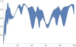
Figure 2: The von Neumann entanglement entropy (3.15) as a function of time for $N=15,s=1,\theta=0.5\pi,A=B=1.0$.

3.3 Spin expectation value

The expectation value of the central spin can be computed using the reduced density matrix

$$\vec{S}(t)=\langle\Psi(t)|\vec{S}|\Psi(t)\rangle=\mathop{\rm tr}\nolimits\left[\vec{S}\,\rho(t)\right]\,.$$ (3.17)

In particular, the so-called spin polarization is given in terms of the diagonal elements of (3.14)

$$S^{z}(t)=\sum_{n=0}^{N}\sum_{j,l,l^{\prime}=0}^{2s}{N\choose n}\cos^{2(N-n)}(\tfrac{\theta}{2})\sin^{2n}(\tfrac{\theta}{2})\,(s-j)\,c_{j,l}^{(s)}(n)\,c_{j,l^{\prime}}^{(s)}(n)\,e^{-it\left(\omega_{l}^{(s)}(n)-\omega_{l^{\prime}}^{(s)}(n)\right)}\,.$$ (3.18)

An example of the spin polarization for $s=1$ is presented in Fig. 3. In contrast with the $s=\frac{1}{2}$ case [15], the duration of collapses quickly tend to zero as $t$ increases. This indicates that the bath is mixing all the states of the central spin. Note also that, for spin $s$, the revival regions consist of up to $2s+1$ revival peaks.

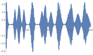
Figure 3: The spin polarization of the central spin (3.18) as a function of time for $N=15,s=1,\theta=0.5\pi,A=B=1.0$.

On the other hand, the so-called coherent factor $S^{-}(t)=\langle\Psi(t)|S^{-}|\Psi(t)\rangle$ involves off-diagonal elements of the reduced density matrix, an example of which is presented in Fig. 4.

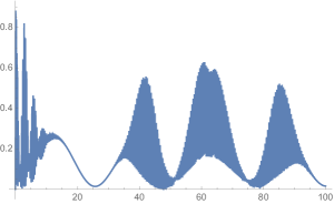
Figure 4: The squared norm coherent factor of the central spin $|S^{-}(t)|^{2}$ as a function of time for $N=15,s=1,\theta=0.5\pi,A=B=1.0$.

3.4 Loschmidt echo

The Loschmidt echo can also be readily computed using the result (3.8)

$$L(t)\equiv|\langle\Psi(0)|\Psi(t)\rangle|^{2}=\left|\sum_{n=0}^{N}{N\choose n}\cos^{2(N-n)}(\tfrac{\theta}{2})\sin^{2n}(\tfrac{\theta}{2})\sum_{l=0}^{2s}c_{0,l}^{(s)}(n)\,e^{-it\omega_{l}^{(s)}(n)}\right|^{2}\,.$$ (3.19)

The fact that $L(0)=1$ is ensured by the second identity in (3.10).

An example of the Loschmidt echo $L(t)$ for $s=1$ is presented in Fig. 5. In contrast with the $s=\frac{1}{2}$ case [15], here $L(t)$ displays rapid irregular oscillations. Notice the appearance of points when $L(t)=0$, at which times the states are completely orthogonal to the initial state.

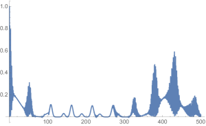
Figure 5: The Loschmidt echo (3.19) as a function of time for $N=15,s=1,\theta=0.5\pi,A=B=1.0$.

4 Conclusions

We have presented two approaches for determining the exact spectrum of the spin-$s$ homogeneous central spin model. The first approach, based on properties of $SU(2)$, leads to the reduced eigenvalue problem (2.13). The second approach, based on integrability, leads to the Bethe ansatz solution (2.30) and (2.31); however, it remains to be understood whether this solution can give the full spectrum.

We have also performed an exact analysis of the time evolution of a spin coherent state, leading to the result (3.8). This allows us to compute the time evolution of various quantities of physical interest, including the entanglement entropy (3.15), spin polarization (3.18) and Loschmidt echo (3.19). For $s>\frac{1}{2}$, we have found interesting differences in comparison with the $s=\frac{1}{2}$ case [15]. While we have restricted for simplicity to the case that the central spin is initially “up”, it should be possible to generalize this analysis to other cases, such as the GHZ [36]-like state $(|s,s\rangle+|s,-s\rangle)/\sqrt{2}$, or states corresponding to entangled states of lower spin. We expect that this model can help usher in the era of tunable quantum metrology.

Appendix A Computation of the coefficients $h^{(s,k)}_{j}$

Here we compute the important coefficients $h^{(s,k)}_{j}$ appearing in (3.6). Our strategy is to determine these coefficients by means of recurrence relations. Acting on both sides of (3.6) with the Hamiltonian $H^{(s)}$, we obtain

$$(H^{(s)})^{k+1}\left(|s,s\rangle\otimes|n\rangle\right) =\sum_{j=0}^{2s}h^{(s,k)}_{j}H^{(s)}\left(|s,s-j\rangle\otimes|n-j\rangle\right)$$

$$=\sum_{j=0}^{2s}h^{(s,k+1)}_{j}|s,s-j\rangle\otimes|n-j\rangle\,.$$ (A.1)

Writing the Hamiltonian in terms of spin raising and lowering operators (2.9) and making use of (2.10), we arrive at a system of recurrence relations

$$h^{(s,k+1)}_{j}=\alpha_{j}^{(s)}\,h^{(s,k)}_{j}+\beta_{j}^{(s)}\,h^{(s,k)}_{j+1}+\beta_{j-1}^{(s)}\,h^{(s,k)}_{j-1}\,,\qquad h^{(s,0)}_{j}=\delta_{j,0}\,,\qquad j=0,1,\ldots,2s\,,$$ (A.2)

whose coefficients are given by

$$\alpha_{j}^{(s)} =B(s-j)+2A(s-j)(\frac{N}{2}+j-n)\,,$$

$$\beta_{j}^{(s)} =A\sqrt{(j+1)(2s-j)(n-j)(N+j+1-n)}\,.$$ (A.3)

In order to solve these recurrence relations, we define the generating functions

$$h_{j}^{(s)}(z)=\sum_{k=0}^{\infty}h^{(s,k)}_{j}z^{k}\,.$$ (A.4)

By virtue of (A.2), these generating functions satisfy a system of linear relations

$$(\alpha_{j}^{(s)}-\frac{1}{z})\,h_{j}^{(s)}(z)+\beta_{j}^{(s)}\,h_{j+1}^{(s)}(z)+\beta_{j-1}^{(s)}\,h_{j-1}^{(s)}(z)=-\frac{1}{z}\delta_{j,0}\,,\qquad j=0,1,\ldots,2s\,,$$ (A.5)

which we can also write in matrix form

$$M^{(s)}(z)\,h^{(s)}(z)=C^{(s)}(z)\,,$$ (A.6)

where we have introduced the column vectors $h^{(s)}(z)=(h_{0}^{(s)}(z),\ldots,h_{2s}^{(s)}(z))^{T}$ and $C^{(s)}(z)=(-\frac{1}{z},0,\ldots,0)^{T}$, and $M^{(s)}(z)$ is the tridiagonal matrix

$$M^{(s)}(z)=\left(\begin{array}[]{ccccccc}\alpha_{0}-\frac{1}{z}&\beta_{0}&0&0&\ldots&0&0\\ \beta_{0}&\alpha_{1}-\frac{1}{z}&\beta_{1}&0&\ldots&0&0\\ 0&\beta_{1}&\alpha_{2}-\frac{1}{z}&\beta_{2}&\ldots&0&0\\ \vdots&\vdots&\vdots&\vdots&&\vdots&\vdots\\ 0&0&0&0&\ldots&\beta_{2s-1}&\alpha_{2s}-\frac{1}{z}\end{array}\right)_{(2s+1)\times(2s+1)}\,.$$ (A.7)

The solutions of the relations (A.5) are given by the following rational functions of $z$

$$h_{j}^{(s)}(z)=\frac{\sum_{l=0}^{2s}n_{l}^{(s,j)}z^{l}}{\sum_{l=0}^{2s+1}d_{l}^{(s)}z^{l}}\,,\qquad j=0,1,\ldots,2s\,.$$ (A.8)

The coefficients in the denominator $d_{l}^{(s)}$ can be read off from an expansion of the determinant of the matrix $M^{(s)}(z)$ (A.7) in inverse powers of $z$,

$$\det\left(M^{(s)}(z)\right)=\sum_{l=0}^{2s+1}\frac{(-1)^{2s+1}}{z^{2s+1-l}}d^{(s)}_{l}\,,\qquad d_{0}^{(s)}=1\,.$$ (A.9)

Note that $d^{(s)}_{l}$ is independent of the value of $j$ in (A.8). The coefficients in the numerator $n_{l}^{(s,j)}$, which do depend on the value of $j$, can be read off from a similar expansion of the minors of the first row of the matrix $M^{(s)}(z)$,

$${\rm minor}_{(1,1+j)}\left(M^{(s)}(z)\right)=\sum_{l=0}^{2s}\frac{(-1)^{2s+j}}{z^{2s-l}}n^{(s,j)}_{l}\,,\qquad n^{(s,j)}_{0}=\delta_{j,0}\,,\qquad j=0,1,\ldots,2s\,.$$ (A.10)

Clearly, both $d^{(s)}_{l}$ and $n_{l}^{(s,j)}$ are expressed in terms of the $\alpha$’s and $\beta$’s (A.3).

Performing a partial fraction decomposition of the solutions $h_{j}^{(s)}(z)$ (A.8), we obtain

$$h_{j}^{(s)}(z)=\sum_{l=0}^{2s}\frac{c_{j,l}^{(s)}}{1-\omega_{l}^{(s)}z}\,,$$ (A.11)

where $\omega_{l}^{(s)}$ is the $(l+1)^{th}$ root of the following polynomial equation of degree $2s+1$

$$\sum_{i=0}^{2s+1}d_{i}^{(s)}\,z^{2s+1-i}=0\,.$$ (A.12)

Moreover, we obtain formulas for $c_{j,l}^{(s)}$ by evaluating the residues of $h_{j}^{(s)}(z)$ (A.8) at $z=1/\omega_{l}^{(s)}$,

$$c_{j,l}^{(s)}=\frac{\sum_{i=0}^{2s}n_{i}^{(s,j)}\left(\omega_{l}^{(s)}\right)^{2s-i}}{\prod_{i=1,i\neq l}^{2s+1}(\omega_{l}^{(s)}-\omega_{i}^{(s)})}\,.$$ (A.13)

In view of the definition (A.4) of the generating functions, the sought-after coefficients $h_{j}^{(s,k)}$ can be obtained from

$$h_{j}^{(s,k)}=\frac{1}{k!}\frac{d^{k}}{dz^{k}}h_{j}^{(s)}(z)\Big{|}_{z=0}\,.$$ (A.14)

Performing this computation using the solution (A.11), we conclude that

$$h_{j}^{(s,k)}=\sum_{l=0}^{2s}c_{j,l}^{(s)}\,\left(\omega_{l}^{(s)}\right)^{k}\,,\qquad j=0,1,\ldots,2s\,.$$ (A.15)

As a consistency check, note that substituting the result (A.15) back into (A.4) and interchanging the order of summations, one obtains

$$h_{j}^{(s)}(z)=\sum_{l=0}^{2s}c_{j,l}^{(s)}\left[\sum_{k=0}^{\infty}\left(\omega_{l}^{(s)}z\right)^{k}\right]\,.$$ (A.16)

Summing the geometric series in (A.16), one recovers the result (A.11).

In short, we have the following recipe for computing the coefficients $h_{j}^{(s,k)}$ appearing in (3.6):

1. Construct the matrix $M^{(s)}(z)$ (A.7), where the $\alpha$’s and $\beta$’s are defined in (A.3).

2. Read off $d_{l}^{(s)}$ and $n_{l}^{(s,j)}$ using (A.9) and (A.10), respectively.

3. Solve the polynomial equation (A.12) to obtain $\omega_{l}^{(s)}$.

4. Obtain $c_{j,l}^{(s)}$ using (A.13).

5. Obtain $h_{j}^{(s,k)}$ using (A.15).

It is straightforward to implement this recipe numerically on a computer.

Note that $\omega_{l}^{(s)}$ and $c_{j,l}^{(s)}$ also depend on $n$, $N$, $A$, and $B$ (through the $\alpha$’s and $\beta$’s), but we have not explicitly displayed these dependences here in order to lighten the notation. However, we do display the dependence on $n$ in the corresponding formula in the body of the paper (3.7), due to the presence there of a summation over $n$.

Appendix B Identities for $c_{j,l}^{(s)}$

We obtain here some useful identities for the coefficients $c_{j,l}^{(s)}$ appearing in $h_{j}^{(s,k)}$ (A.15). We begin by evaluating the generating functions $h_{j}^{(s)}(z)$ at $z=0$ in two different ways: using (A.8) we obtain

$$h_{j}^{(s)}(0)=\frac{n_{0}^{(s,j)}}{d_{0}^{(s)}}=\delta_{j,0}\,,$$ (B.1)

while (A.11) gives

$$h_{j}^{(s)}(0)=\sum_{l=0}^{2s}c_{j,l}^{(s)}\,.$$ (B.2)

We conclude from (B.1) and (B.2) that

$$\sum_{l=0}^{2s}c_{j,l}^{(s)}=\delta_{j,0}\,.$$ (B.3)

Multiplying both sides of (B.3) by $c_{j,l^{\prime}}^{(s)}$ and summing over $j$, we obtain

$$\sum_{j=0}^{2s}\sum_{l=0}^{2s}c_{j,l}^{(s)}\,c_{j,l^{\prime}}^{(s)}=c_{0,l^{\prime}}^{(s)}\,.$$ (B.4)

Let us now evaluate the expression $\sum_{j=0}^{2s}h_{j}^{(s)}(z)\,h_{j}^{(s)}(z^{\prime})$ in two different ways. Using (A.11) we obtain

$$\sum_{j=0}^{2s}h_{j}^{(s)}(z)\,h_{j}^{(s)}(z^{\prime})=\sum_{j=0}^{2s}\sum_{l,l^{\prime}=0}^{2s}\frac{c_{j,l}^{(s)}\,c_{j,l^{\prime}}^{(s)}}{(1-\omega_{l}^{(s)}z)(1-\omega_{l^{\prime}}^{(s)}z^{\prime})}\,.$$ (B.5)

On the other hand, we know from (A.6) that $h^{(s)}(z)=(M^{(s)}(z))^{-1}\,C^{(s)}(z)$. Therefore,

$$\sum_{j=0}^{2s}h_{j}^{(s)}(z)\,h_{j}^{(s)}(z^{\prime})=\frac{1}{zz^{\prime}}\left(M(z)M(z^{\prime})\right)^{-1}_{00}\,.$$ (B.6)

Since $\det(M(z))$ does not vanish at $z=\omega_{l}^{(s)}$ (it vanishes instead at $z=1/\omega_{l}^{(s)}$), and similarly for $\det(M(z^{\prime}))$, we see from (B.6) that $\sum_{j=0}^{2s}h_{j}^{(s)}(z)\,h_{j}^{(s)}(z^{\prime})$ is regular at $z=\omega_{l}^{(s)}\,,z^{\prime}=\omega_{l^{\prime}}^{(s)}$. Evaluating the residues of both sides of (B.5) at $z=\omega_{l}^{(s)}\,,z^{\prime}=\omega_{l^{\prime}}^{(s)}$ with $l\neq l^{\prime}$, we obtain

$$\sum_{j=0}^{2s}c_{j,l}^{(s)}\,c_{j,l^{\prime}}^{(s)}=0\,,\qquad l\neq l^{\prime}\,.$$ (B.7)

Combining this result with (B.4), we conclude that

$$\sum_{j=0}^{2s}c_{j,l}^{(s)}\,c_{j,l^{\prime}}^{(s)}=c_{0,l}^{(s)}\,\delta_{l,l^{\prime}}\,.$$ (B.8)

The main results of this appendix are the identities (B.3) and (B.8).

References

- [1] R. W. Richardson, “A restricted class of exact eigenstates of the pairing-force Hamiltonian,” Phys. Lett 3 (1963) 277–279.
- [2] R. W. Richardson and N. Sherman, “Exact eigenstates of the pairing-force Hamiltonian,” Nucl. Phys. 52 (1964) 221–238.
- [3] M. Gaudin, “Diagonalization of a class of spin Hamiltonians,” J. Physique 37 (1976) 1087–1098.
- [4] M. Gaudin, La fonction d’onde de Bethe. Masson, 1983. English translation by J.-S. Caux, The Bethe Wavefunction, Cambridge University Press, 2014.
- [5] A. V. Khaetskii, D. Loss, and L. Glazman, “Electron spin decoherence in quantum dots due to interaction with nuclei,” Phys. Rev. Lett. 88 (2002) 186802, cond-mat/0201303.
- [6] I. A. Merkulov, A. L. Efros, and M. Rosen, “Electron spin relaxation by nuclei in semiconductor quantum dots,” Phys. Rev. B 65 (2002) 205309, cond-mat/0202271.
- [7] A. V. Khaetskii, D. Loss, and L. Glazman, “Electron spin evolution induced by interaction with nuclei in a quantum dot,” Phys. Rev. B 67 (2003) 195329, cond-mat/0211678.
- [8] S. I. Erlingsson and Y. V. Nazarov, “Evolution of localized electron spin in a nuclear spin environment,” Phys. Rev. B 70 (2004) 205327.
- [9] P.-F. Braun, X. Marie, L. Lombez, B. Urbaszek, T. Amand, P. Renucci, V. K. Kalevich, K. V. Kavokin, O. Krebs, P. Voisin, and Y. Masumoto, “Direct observation of the electron spin relaxation induced by nuclei in quantum dots,” Phys. Rev. Lett. 94 (2005) 116601.
- [10] G. Chen, D. L. Bergman, and L. Balents, “Semiclassical dynamics and long-time asymptotics of the central-spin problem in a quantum dot,” Phys. Rev. B 76 (2007) 045312, cond-mat/0703631.
- [11] M. Bortz and J. Stolze, “Exact dynamics in the inhomogeneous central-spin model,” Phys. Rev. B 76 (2007) 014304, cond-mat/0612382.
- [12] M. Bortz, S. Eggert, C. Schneider, R. Stubner, and J. Stolze, “Dynamics and decoherence in the central spin model using exact methods,” Phys. Rev. B 82 (2010) 161308, 1005.0001.
- [13] S. Dooley, F. McCrossan, D. Harland, M. J. Everitt, and T. P. Spiller, “Collapse and revival and cat states with an -spin system,” Phys. Rev. A 87 (2013) 052323, arXiv:1302.2806 [quant-ph].
- [14] W.-B. He and X.-W. Guan, “Exact results of quantum dynamics of Gaudin models,” in preparation.
- [15] W.-B. He, S. Chesi, H.-Q. Lin and X.-W. Guan, “Exact quantum dynamics of XXZ central spin problems,” arXiv:1810.03012 [quant-ph].
- [16] E. T. Jaynes and F. W. Cummings, “Comparison of quantum and semiclassical radiation theories with application to the beam maser,” Proc. IEEE 51 (1963) 89–109.
- [17] M. O. Scully and M. S. Zubairy, Quantum Optics. Cambridge University Press, 1997.
- [18] N. M. Bogoliubov and P. P. Kulish, “Exactly solvable models of nonlinear quantum optics,” J. Math. Sciences 192 (2013) 14–30.
- [19] M. Tavis and F. W. Cummings, “Exact solution for an N-molecule radiation-field Hamiltonian,” Phys. Rev. 170 (1968) 379–384.
- [20] M. Knap, E. Arrigoni, and W. von der Linden, “Quantum phase transition and excitations of the Tavis-Cummings lattice model,” Phys. Rev. B 82 (2010) 045126.
- [21] M. Youssef, N. Metwally, and A.-S. F. Obada, “Some entanglement features of a three-atom Tavis Cummings model: a cooperative case,” J. Phys. B: At. Mol. Opt. Phys 43 (2010) 095501.
- [22] S. Agarwal, S. M. Hashemi Rafsanjani, and J. H. Eberly, “Tavis-Cummings model beyond the rotating wave approximation: Quasidegenerate qubits,” Phys. Rev. A 85 (2012) 043815.
- [23] E. K. Sklyanin, “Separation of variables in the Gaudin model,” J. Sov. Math. 47 (1989) 2473–2488. [Zap. Nauchn. Semin.164, 151 (1987)].
- [24] K. Hikami, P. P. Kulish, and M. Wadati, “Integrable spin systems with long range interactions,” J. Phys. Soc. Jap. 61 (1992) 3071–3076.
- [25] H.-Q. Zhou, J. Links, R. H. McKenzie, and M. D. Gould, “Superconducting correlations in metallic nanoparticles: Exact solution of the BCS model by the algebraic Bethe ansatz,” Phys. Rev. B 65 (2002) 060502, arXiv:0106390 [cond-mat.supr-con].
- [26] H. M. Babujian, “Exact solution of the isotropic Heisenberg chain with arbitrary spins: thermodynamics of the model,” Nucl. Phys. B215 (1983) 317–336.
- [27] J. Links, “Completeness of the Bethe states for the rational, spin-1/2 Richardson–Gaudin system,” SciPost Phys. 3 (2017) 007, arXiv:1603.03542 [nlin.SI].
- [28] W. Hao, R. I. Nepomechie, and A. J. Sommese, “Completeness of solutions of Bethe’s equations,” Phys. Rev. E88 no. 5, (2013) 052113, arXiv:1308.4645 [math-ph].
- [29] M. Gaudin, “Boundary Energy of a Bose Gas in One Dimension,” Phys. Rev. A4 (1971) 386–394.
- [30] S. Shastry and A. Dhar, “Solution of a generalized Stieltjes problem,” J.Phys. A34 (2001) 6197, arXiv:cond-mat/0101464 [cond-mat].
- [31] X. Guan, K. D. Launey, M. Xie, L. Bao, F. Pan, and J. P. Draayer, “Heine-Stieltjes correspondence and the polynomial approach to the standard pairing problem,” Phys.Rev. C86 (2012) 024313, arXiv:1106.5237 [nucl-th].
- [32] I. Marquette and J. Links, “Generalised Heine-Stieltjes and Van Vleck polynomials associated with degenerate, integrable BCS models,” J.Stat.Mech. P08019 (2012) , arXiv:1206.2988 [nlin.SI].
- [33] T. Holstein and H. Primakoff, “Field dependence of the intrinsic domain magnetization of a ferromagnet,” Phys. Rev. 58 (1940) 1098–1113.
- [34] J. M. Radcliffe, “Some properties of coherent spin states,” J. Phys. A 4 (1971) 313.
- [35] F. T. Arecchi, E. Courtens, R. Gilmore, and H. Thomas, “Atomic coherent states in quantum optics,” Phys. Rev. A 6 (1972) 2211–2237.
- [36] D. M. Greenberger, M. Horne, and A. Zeilinger, “Bell s theorem without inequalities,” Am. J. Phys 58 (1990) 1131.