Topological approach to quantum liquid ground states on geometrically frustrated Heisenberg antiferromagnets

Abstract

We have formulated a twist operator argument for the geometrically frustrated quantum spin systems on the kagome and triangular lattices, thereby extending the application of the Lieb-Schultz-Mattis (LSM) and Oshikawa-Yamanaka-Affleck (OYA) theorems to these systems. The equivalent large gauge transformation for the geometrically frustrated lattice differs from that for non-frustrated systems due to the existence of multiple sublattices in the unit cell and non-orthogonal basis vectors. Our study for the $S=1/2$ kagome Heisenberg antiferromagnet at zero external magnetic field gives a criterion for the existence of a two-fold degenerate ground state with a finite excitation gap and fractionalized excitations. At finite field, we predict various plateaux at fractional magnetisation, in analogy with integer and fractional quantum Hall states of the primary sequence. These plateaux correspond to gapped quantum liquid ground states with a fixed number of singlets and spinons in the unit cell. A similar analysis for the triangular lattice predicts a single fractional magnetization plateau at $1/3$. Our results are in broad agreement with numerical and experimental studies.

I Introduction

Frustrated spin systems have, for several decades, drawn significant attention in the search for exotic ground states. The causes of frustration are several Anderson (1973, 1987); Ceccatto et al. (1992); Kitaev (2006), with special emphasis given to lattices on which the classical Néel ground states of the nearest neighbour (n.n) Heisenberg antiferromagnet cannot be stabilised due to an intrinsic frustration. The kagome and triangular lattices in 2D and the pyrochlore lattice in 3D are classic examples of such systems. A large number of theoretical as well as experimental studies have sought novel ground states such as spin liquids and spin ice Lee (2008); Balents (2010); Norman (2016), as well as states possessing topological order and fractionalized excitations Han et al. (2012). In spite of extensive studies on the $S=1/2$ Heisenberg kagome antiferromagnet (HKA), the nature of the ground state and the existence of a spectral gap remain inconclusive. Some studies support the existence of a gap and short-ranged resonating valence bond (RVB) order Xie et al. (2014); Mei et al. (2017); Jiang et al. (2012); Fu et al. (2015); Yan et al. (2011); Isakov et al. (2006), while others suggest a gapless spectrum and algebraic order Ran et al. (2007); Ryu et al. (2007); Iqbal et al. (2011, 2013, 2014); Liao et al. (2017); He et al. (2017). Another interesting aspect of geometrically frustrated spin systems is that they can possess nontrivial plateaux at zero and fractional magnetisation (see, e.g., Schulenburg et al. (2002); Honecker et al. (2004); Schnack et al. (2018); Zhitomirsky and Tsunetsugu (2004); Nakano and Sakai (2010); Chubokov and Golosov (1991); Hida (2001); Nishimoto et al. (2013); Ishikawa et al. (2015); Alicea et al. (2009); Ono et al. (2003) for triangular and kagome lattices). The existence of such plateaux indicates a finite gap in the energy spectrum and the possibility of ground states with non-trivial topological features analogous to the quantum Hall effects Oshikawa et al. (1997); Kumar et al. (2016, 2015); Tao and Wu (1984). In fact, the ground state wavefunction for the plateau at fractional magnetization $m=7/9$ is known exactly Schulenburg et al. (2002); Zhitomirsky and Tsunetsugu (2004); Changlani et al. (2019).

There exist very few methods that, relying solely on the symmetries of the Hamiltonian, can offer qualitative insight on the nature of the ground state and the low-energy excitation spectrum. One of these is the Lieb-Schultz-Mattis (LSM) theoremLieb et al. (1961). Originally formulated for the spin-$1/2$ n.n. Heisenberg antiferromagnet chain, it was extended to higher dimensions for geometrically non-frustrated systems more recently Affleck (1988); Oshikawa (2000a); Hastings (2004). The theorem relates the existence (or lack) of a spectral gap to the sensitivity of the ground state to adiabatic changes in boundary conditions implemented by a twist operator. A degeneracy of the ground state can also be gauged from the non-commutativity between the lattice translation and twist operators. Recent works have been devoted to extending the applicability of the LSM theorem to systems with a variety of interactions (e.g., extended, anisotropic, bond-alternating, Dzyaloshinskii-Moriya and even frustrating) Nomura et al. (2015); Isoyama and Nomura (2017); Tasaki (2018). This is in broad agreement with some numerical studies of (quasi-)one dimensional systems (e.g., chains and ladders) Florek et al. (2016); Antkowiak et al. (2017); Florek (2018). These works indicate that the minimum requirements for the LSM theorem are spin Hamiltonians possessing $U(1)$ spin symmetry, translation invariance in real space and short-ranged interactions. Importantly, without assuming either a bipartite lattice or a unique ground state, Ref.(Nomura et al. (2015)) extends the LSM theorem to frustrated spin systems in quasi-one dimension where ground states may be degenerate. Further, Oshikawa et al.  Oshikawa et al. (1997) extended the LSM-theorem to the case of finite magnetization (the OYA criterion), using which one can predict possible magnetization plateaux for finite external magnetic field. It is important to note that the OYA-criterion has been extended to quantum antiferromagnetic systems in abitrary spatial dimensions by Tanaka et al. Tanaka et al. (2009); Tanaka and Takayoshi (2015) with the help of effective field theory and renormalisation group (RG) analyses. Further, the OYA-criterion has been successful in predicting plateaux for the $S=1/2$ HKA Fledderjohann et al. (1999); Capponi et al. (2013); Nishimoto et al. (2013). Very recently, two of us have predicted possible magnetization plateau states in $S=1/2$ pyrochlore lattice by using a similar formalism to that presented herePal and Lal (2019). In a RG analysis of the $S=1/2$ HKA on the kagome lattice (Pal et al., 2019), we have also shown that the twist operator we present here is responsible for the formation of the spectral gap that protects the $1/3$ magnetization plateau ground state. This provides important evidence for the origin of the spectral gap assume in the twist operator based analysis.

As presented in Section II, the main goal of the present work is to define the twist operator (also called a large gauge transformation operator Oshikawa (2000a); Paramekanti and Vishwanath (2004)) for geometrically frustrated 2D lattices (e.g., kagome and triangular). The subtlety in the form of the twist operator in such lattices lies in identifying the non-trivial unit cell and the associated basis vectors. Then, from the usual non-commutativity between twist and translation operators, we obtain the possibility of gapped, doubly-degenerate ground states with interpolating fractional excitations for the HKA at zero field in Section III. Further, in sections III and IV, we demonstrate the existence of several plateaux at finite magnetisation from an OYA-like criterion on the kagome and triangular lattices. These compare favourably with results obtained from various numerical methods Nishimoto et al. (2013). The non-saturation plateaux obtained at non-zero field from such spectral flow arguments correspond to quantum liquid ground states in which the unit cells comprise of short-ranged RVBs along with a fixed number of spinon excitations  Altman and Auerbach (1998); Kumar et al. (2015). This should be contrasted with proposals of quantum solid valence bond solid (VBS) ground states Affleck et al. (1987) and $SU(2)$ symmetry broken classical ground states Sachdev (1992) for geometrically frustrated 2D spin systems. We conclude in Section V, presenting some open directions. For the sake of completeness, we present the details of the calculations for the energy cost related to the twist operation and the LSM-like theorem for the kagome lattice in Appendices A and B.

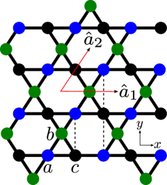
Figure 1: Schamatic diagram of kagome lattice with the basis vectors $\hat{a}_{1}=\hat{x},\hat{a}_{2}=\frac{1}{2}\hat{x}+\frac{\sqrt{3}}{2}\hat{y}$, so the distance between nearest neighbour sites is half. Every triangular unit cell has three different sublattice labelled by $a,b$ and $c$ ( blue, green and black respectively). The dashed lines show the non-zero projection of sites in the $\hat{a}_{2}$ direction along $\hat{a}_{1}$.

II Twist Operator for the kagome lattice

The kagome system has two basis vectors $\hat{a}_{1}$ and $\hat{a}_{2}$ with which the complete lattice can be spanned [Fig.(1)]. The Hamiltonian for $S=\frac{1}{2}$ n.n HKA in a field $h$ is Hermele et al. (2008)

$$H=J\sum_{<\vec{r}\vec{r}^{\prime}>}\vec{S}_{\vec{r}}\cdot\vec{S}_{\vec{r}^{\prime}}-h\sum_{\vec{r}}\hat{S}^{z}_{\vec{r}}~{},$$ (1)

where the spin exchange $J>0$ and sum is over n.n sites. Here $\vec{r}\in(\vec{R},j)$, with $\vec{R}=n_{1}\hat{a}_{1}+n_{2}\hat{a}_{2}$ ($n_{1},n_{2}$ are integer) the lattice vector for a three sub-lattice unit cell (up triangles) and $j\in{(a,b,c)}$ are the three sub-lattices. For $N_{1}$ and $N_{2}$ being the number of each sub-lattice along the $\hat{a}_{1}$ and $\hat{a}_{2}$ directions respectively, the total number of sites in the lattice is $3N_{1}N_{2}$. Below, we will consider periodic boundary conditions (PBC) along $\hat{a}_{1}$ direction. Now, for $\delta$ being the distance between n.n sites, $L_{\hat{a}_{1}}=2\delta N_{1}$ and $L_{\hat{a}_{2}}=2\delta N_{2}$ are the lengths along the $\hat{a}_{1}$ and $\hat{a}_{2}$ directions respectively. Hereafter, we will consider $\delta=1$.

In the LSM theorem Lieb et al. (1961), a twist (i.e., a change in boundary conditions) is equivalent to insertion of an Aharanov-Bohm (AB) flux Oshikawa (2000a); Paramekanti and Vishwanath (2004) that generates a vector potential along the periodic direction. This is analogous to Laughlin’s flux insertion for the quantum Hall effect Laughlin (1981). By this argument, one can extend the LSM theorem to higher dimensions Hastings (2004), with twisting equivalent to a large gauge transformation of the Hamiltonian. We expect an invariance of the spectrum under a large gauge transformation equivalent to the adiabatic insertion of a full flux quanta ($2\pi$, in units $h=c=e=1$). The twisted wavefunction, however, reveals the effect of the flux. Thus, we compute a shift in the crystal momentum by applying a gauge transformation that reverses precisely the shift in the eigenspectrum due to the flux Paramekanti and Vishwanath (2004). This shift is revealed by a non-commutativity between the translation and twist operators.

In applying the LSM theorem on geometrically frustrated lattices, one has to be careful in defining a suitable large gauge transformation. On such lattices, the basis vectors are usually not orthogonal to one another (see Fig.(1) for the kagome lattice). Therefore, spins at different sites along a basis vector (other than that along which the twist is applied) differ in the phase induced by the equivalent AB flux. We place the system shown in Fig.(1) on a cylinder, with PBC along $\hat{x}\equiv\hat{a}_{1}$. Now if we apply an AB-flux along the axis of the cylinder, a time-varying vector potential will be induced along $\hat{a}_{1}$ direction. For a uniform gauge $A(x)=2\pi/L_{\hat{a}_{1}}$ and $A(y)=0$, there will be no change in the phase of spins on sites with the same $y$-coordinate. Given that $\hat{a}_{2}$ does not coincide with $\hat{y}$, the phase acquired by the spins varies along $\hat{a}_{2}$. Below, we account for this subtlety in constructing twist operators for the kagome and triangular lattices.

Given that $[S^{\alpha}_{\vec{r}},S^{\beta}_{\vec{r}^{\prime}}]=0$ for $\vec{r}\neq\vec{r}^{\prime}$, where $\alpha,\beta\in\{x,y,z\}$, we can define separate twist operators for the three sub-lattices ($\hat{O}_{a}$, $\hat{O}_{b}$ and $\hat{O}_{c}$) and combine them for the complete twist operator $\hat{O}=\hat{O}_{a}\hat{O}_{b}\hat{O}_{c}$ . Then, for a flux quantum along $\hat{y}$, the phase difference between spins belonging to the nearest sites of the same sub-lattice and with fixed $n_{2}$ ($n_{1}$) coordinate is given by $2\pi/N_{1}$ ($\pi/N_{1}$); see dashed lines in Fig.(1). Therefore, with the site marked as $a$ in Fig.(1) chosen as the reference site, the twist operator for sub-lattice $a$ ($\hat{O}_{a}$) is given by

$$\hat{O}_{a}=\exp\big{[}i\frac{2\pi}{N_{1}}\sum_{\vec{R}}(n_{1}+\frac{n_{2}}{2})\hat{S}^{z}_{\vec{R},a}\big{]}~{}.$$ (2)

In a given unit cell, the phases acquired by $b$ and $c$ sub-lattices differ by $\frac{1}{4}(2\pi/N_{1})$ and $\frac{1}{2}(2\pi/N_{1})$ respectively with respect to the $a$ sub-lattice. Thus, the twist operator for sub-lattice $b$ is given by

$$\hat{O}_{b} = \exp\big{[}i\frac{2\pi}{N_{1}}\sum_{\vec{R}}(n_{1}+\frac{n_{2}}{2}+\frac{1}{4})\hat{S}^{z}_{\vec{R},b}\big{]}~{},$$ (3)

while $\hat{O}_{c}$ is identical in form, with only the term proportional to $1/4$ in the exponent replaced by one proportional to $1/2$. Combining the three, we obtain the complete twist operator for kagome lattice

$$\hat{O}=\exp\big{[}i\frac{2\pi}{N_{1}}\Big{(}\sum_{\vec{r}}(n_{1}+\frac{n_{2}}{2})\hat{S}^{z}_{\vec{r}}+\sum_{\vec{R}}(\frac{1}{4}\hat{S}^{z}_{\vec{R},b}+\frac{1}{2}\hat{S}^{z}_{\vec{R},c})\Big{)}\big{]}.$$ (4)

This form of the twist operator differs from that obtained for non-frustrated lattices Oshikawa (2000a); Paramekanti and Vishwanath (2004) in two ways. The term proportional to $n_{2}$ appears due to the non-orthogonality of the basis vectors, while the terms proportional to $\hat{S}^{z}_{\vec{R},b}$ and $\hat{S}^{z}_{\vec{R},c}$ arise due to the different phase twists acquired by the sub-lattices of the kagome system. We will use this twist operator to obtain the nature of the ground state and low-energy spectrum for the HKA. In Appendix A, we show that the excitation gap between the ground state and the twisted state vanishes in the thermodynamic limit for a vanishing spin stiffness Hastings (2004); Misguich et al. (2002).

III LSM-like theorem and OYA-like criterion for the kagome lattice

We denote the unit translation operator along $\hat{a}_{1}$ direction as $\hat{T}_{\hat{a}_{1}}$, such that $\hat{T}_{\hat{a}_{1}}\hat{S}^{z}_{n_{1},n_{2},j}\hat{T}^{\dagger}_{\hat{a}_{1}}=\hat{S}^{z}_{n_{1}+1,n_{2},j}$ . For PBC along $\hat{a}_{1}$ direction, we obtain the identity (see Appendix B for a detailed calculation)

$$\hat{T}_{\hat{a}_{1}}\hat{O}\hat{T}^{\dagger}_{\hat{a}_{1}}=\hat{O}\exp\big{[}-i\frac{2\pi}{N_{1}}(\hat{S}^{z}_{Tot}-N_{1}N_{2}\hat{S}^{z}_{\triangle})\big{]}~{},$$ (5)

$N_{2}\hat{S}^{z}_{\triangle}$ is the $z$-component of the vector sum of all spins within the $N_{2}$ unit cells where the total magnetization is given by $\hat{S}^{z}_{Tot}=\sum_{\vec{r}}\hat{S}^{z}_{\vec{r}}$. We obtain the factor $N_{2}\hat{S}^{z}_{\triangle}$ as the $z$-component of the vector sum of all spins within the $N_{2}$ unit cells lying on a line along $\hat{a}_{2}$ (the boundary line Paramekanti and Vishwanath (2004)) by assuming translation invariance along that direction. For the kagome lattice, $S_{\triangle}=1/2,3/2$ such that the eigenvalues of $\hat{S}^{z}_{\triangle}$ are $\pm 1/2,\pm 3/2$. As mentioned earlier, the applicability of the LSM theorem demands a $U(1)$ invariance of the ground state, i.e., it is labelled by the eigenvalue of $\hat{S}^{z}_{Tot}$. For the case of $h=0$, the total number of sites in the lattice ($N_{1}\times N_{2}$) has to be even in order to guarantee the time reversal invariance of the ground state, i.e., $\hat{S}^{z}_{Tot}|\psi_{0}\rangle=0$.

Then, at zero field, the matrix element arising from eqn.(5) becomes

$$\langle\psi_{0}|\hat{T}_{\hat{a}_{1}}\hat{O}\hat{T}^{\dagger}_{\hat{a}_{1}}|\psi_{0}\rangle=\langle\psi_{0}|\hat{O}\exp\big{[}-iN_{2}~{}(\text{mod}~{}\pi)\big{]}|\psi_{0}\rangle.$$ (6)

For $N_{2}\in$ odd and the lowest excited state $|\psi_{1}\rangle=\hat{O}|\psi_{0}\rangle$, eqn.(6) leads to $\langle\psi_{0}|\psi_{1}\rangle=0$, i.e., the ground state and the lowest lying excited state are orthogonal to one another. Therefore, employing the LSM argument used for the $S=1/2$ Heisenberg chain as well as ladder systems  Lieb et al. (1961); Altman and Auerbach (1998); Nakamura and Voit (2002), we find that the $S=1/2$ HKA can have one of two possible ground states. The first possibility is that, without the breaking of any symmetries, there exists a many-body gap separating the excitation spectrum from a two-fold degenerate ground state. This is in agreement with the finding of a small zero-magnetization plateau from numerical investigations of the HKA in Ref.(Nishimoto et al. (2013)). These two ground states are topologically separated from one another: the AB flux threading is equivalent to the insertion of a vison carrying a crystal momentum $\pi$ into the hole of the cylinder Paramekanti and Vishwanath (2004). This is the signature of a $Z_{2}$ fractionalised insulating phase Paramekanti and Vishwanath (2004); Moessner et al. (2001); Senthil and Fisher (2000). The degeneracy in the ground state manifold appears in the thermodynamic limit, along with a spin stiffness that decays exponentially with system size Misguich et al. (2002); Altman and Auerbach (1998). This justifies the adiabatic insertion of the AB flux over timescales much longer than the inverse gap Oshikawa (2000a); Hastings (2004); Paramekanti and Vishwanath (2004). The other possibility is that, in the thermodynamic limit, the excitation spectrum generated by $\hat{O}$ collapses, causing the many body gap to vanish. Indeed, another recent work suggests a $U(1)$ gapless spin liquid ground state in the HKA Chen et al. (2018). Thus, the LSM-like arguments presented above are, by construction, unable to resolve between these two possibilities. On the other hand, for $N_{2}\in$ even, $\langle\psi_{0}|\psi_{1}\rangle\neq 0$ and the approach taken here does not yield any firm conclusions about the presence of a gap or ground state degeneracy.

We will now focus on the properties at non-zero magnetic field. Defining magnetization per site as $m=S^{z}_{Tot}/3N_{1}N_{2}$, eqn.(5) becomes

$$\hat{T}_{\hat{a}_{1}}\hat{O}\hat{T}^{\dagger}_{\hat{a}_{1}}=\hat{O}\exp\big{[}-i2\pi(3N_{2})(m-\frac{\hat{S}^{z}_{\triangle}}{3})\big{]}~{}.$$ (7)

The appearance of magnetisation plateaux can be understood by noting that we can write the odd integer $N_{2}$ as the product of two odd numbers, $N_{2}=(2p+1)(2q+1)$ where $(p,q)$ can be zero or any positive integer. Then, denote $3N_{2}=Q_{m}(2q+1)$, where $Q_{m}=3(2p+1)$ corresponds to the size of a magnetic unit cell. The fundamental unit cell of the kagome lattice (see Fig.(1)) has $p=0$ and $Q_{m}=3$ spins, whereas the simplest enlarged unit cell has $p=1$ and $Q_{m}=9$ spins. We can then derive the OYA-like criterion from eqn.(7) in terms of the fractional magnetisation, $m/m_{s}$ (where $m_{s}=1/2$ is the saturation magnetisation per site), by requiring that the argument of the exponential is an integer $n$ (upto a factor of $2\pi(2q+1)$). This is in analogy with the integer quantum Hall effect Oshikawa et al. (1997). Thus, we obtain

$$\frac{Q_{m}}{2}(\frac{m}{m_{s}}-\frac{1}{3})=n\quad\text{or}\quad\frac{Q_{m}}{2}(\frac{m}{m_{s}}-1)=n~{},$$ (8)

for $S^{z}_{\triangle}=1/2$ and for $S^{z}_{\triangle}=3/2$ respectively.

$Q_{m}$	$m/m_{s}$	$S^{z}_{\triangle}=1/2$	$S^{z}_{\triangle}=3/2$
3	$1/3$	$n=0$	$n=-1$
9	$1/9$	$n=-1$	$n=-4$
	$1/3$	$n=0$	$n=-3$
	$5/9$	$n=1$	$n=-2$
	$7/9$	$n=2$	$n=-1$

Table 1: Plateaux in the fractional magnetization ($m/m_{s}$) and the corresponding $(n,S^{z}_{\triangle},Q_{m})$ values in eqn.(8). The symbols are defined in the text.

The table (1) indicates the positions of various plateaux at fractional magnetisation in the HKA. The location of the plateaux agree with results obtained from numerical and experimental works Nishimoto et al. (2013); Capponi et al. (2013); Ishikawa et al. (2015). Motivated by Ref.(Oshikawa et al. (1997)), equn.(8) reveals an analogy between the magnetisation plateaux for $S^{z}_{\triangle}=3/2$ and quantum Hall ground states. For instance, the plateau $m/m_{s}=1/3$ state arising from a fundamental unit cell ($Q_{m}=3$) is analogous to the integer quantum Hall (IQH) state with filling factor $\nu=1$. This argument extends to a unit cell enlargement of $Q_{m}=3(2p+1)$, e.g., the four plateaux arising from the three-fold enlargement ($Q_{m}=9$) are in analogy with fractional quantum Hall (FQH) states with $\nu=|n|/Q_{m}$ Tao and Wu (1984). Further, these ground states contain a fixed number of spinon excitations and RVB singlets Oshikawa (2000b): the fractional magnetisation $m/m_{s}$, the quantity ($Q_{m}m/m_{s})$ and $|n|$ correspond to the spinon density, spinon number and number of singlets within the magnetic unit cell respectively.

We now turn to the plateaux obtained for $S_{\triangle}=1/2=S^{z}_{\triangle}$. The wavefunctions of an isolated triangle of three spin-1/2s (a fundamental unit cell) in the $S_{\triangle}=1/2=S^{z}_{\triangle}$ sector involve linear combinations of states composed of direct products of a given spin-1/2 and the singlet and triplet states of the other two spin-1/2s (see, e.g., eqn. (16) of Ref.(Dai and Whangbo (2004)). Then, the $1/3$ plateau in $Q_{m}=3$ can be seen to arise from wavefunctions composed entirely of linear combinations of direct products of single spin-1/2 and triplet states of the other two spins (i.e., a singlet bond count for the fundamental unit cell being $|n|=0$). For the three-fold enlarged unit cell of $Q_{m}=9$, the $1/9$ and $5/9$ plateau states possess a wavefunction in which one of the three triangles involves a singlet ($|n|=1$). Similarly, the $1/3$ state has a wavefunction with no singlets in any of the three triangles, while the $7/9$ state has singlets in any two triangles.

IV Magnetisation plateaux for the triangular lattice

We now extend our analysis to the triangular lattice. Although the triangular lattice possesses geometrical frustration, it has a simple unit cell with an invariance of the Hamiltonian due to translation by one lattice site. Further, it has two basis vectors identical to the kagome lattice, but with half the length. Thereby, the twist operator for triangular lattice has the form

$$\hat{O}=\exp\big{[}i\frac{2\pi}{N_{1}}\sum_{\vec{R}}(n_{1}+\frac{n_{2}}{2})\hat{S}^{z}_{\vec{R}}\big{]}~{},$$ (9)

with a notation identical to that used for the kagome lattice. Similarly, the OYA-like criterion for the triangular lattice is found to be

$$\frac{Q_{m}}{2}\big{(}\frac{m}{m_{s}}-1\big{)}=n~{}.$$ (10)

This criterion offer a $1/3$-plateau as the simplest possibility via the enlargement of the magnetic unit cell, i.e., with $Q_{m}=3$ and $n=-1$, and is analogous to the FQH state with $\nu=1/3$. This is consistent with predictions from numerical and experimental works  Chubokov and Golosov (1991); Ono et al. (2003, 2003); Alicea et al. (2009); Takano et al. (2011); Yamamoto et al. (2016).

V Conclusions and Outlook

In conclusion, we have derived the twist operator for the kagome and triangular lattices. Although the form of the twist operator is different from that for non-frustrated lattices, the non-commutativity between twist and translation operator is similar in the sense that it depends only on boundary unit cells. We have shown that the contribution from boundary spins leads to several possibilities for magnetization plateaux in frustrated systems. The plateaux are observed to be analogous to the integer and fractional quantum Hall states, offering insight into quantum liquid ground states with fixed numbers of singlets and spinons in the unit cell. While we have focussed on the case of $N_{2}$ being an odd integer in this work, some results can also be obtained for the case of $N_{2}$ being an even integer. For instance, for $Q_{m}=6$, we obtain magnetisation plateaux at $m/m_{s}=0,1/3$ and $2/3$.

There are several interesting directions that are opened by our work. The first involves an investigation of whether the ground state wavefunctions we have obtained for some of the non-trivial magnetisation plateaux correspond to novel topological field theories. For instance, we have recently shown from a renormalisation group analysis that an effective Hamiltonian can be obtained for a quantum spin liquid phase of the Heisenberg quantum antifferomagnet corresponding to the $m/m_{s}=1/3$ plateau in the kagome lattice Pal et al. (2019). This effective Hamiltonian was reached by the condensation of $SU(2)$ symmetric quantum fluctuations, suggesting that the problem can likely be studied in terms of a a $SU(2)$ non-Abelian lattice gauge theory on the kagome lattice associated with such quantum fluctuations Kogut (1979). A continuum version of such a gauge theory is obtained from a fermionic non-linear sigma model of massive Dirac fermions in $(2+1)$ dimensions coupled to a SU(2) order parameter Abanov and Wiegmann (2000), and found to lead to a quantum disordered ground state protected by a dynamically generated mass gap. Further, the theory is topolgical in nature, possessing a topological Hopf term in the effective action. It appears relevant, therefore, to investigate whether any the ground state wavefunction obtained by us for the plateau at $m/m_{s}=1/3$ in this work could be that for the quantum spin liquid ground state of Ref.Pal et al. (2019).

In a recent work  Pal and Lal (2019), the formalism developed here has been extended to the search for magnetization plateaus in other frustrated lattices, e.g., the pyrochlore in 3D. Any results obtained from a twist-operator based approach can likely provide considerable assistance in the experimental search for quantum spin liquids currently being sought in magnetic materials with frustrated geometries. Finally, we hope that this work will also motivate the search for plateaus that correspond to fractional values of the parameter $n$, in analogy with the fractional quantum Hall effect.

Appendix A Energy cost of the Twisted state

Here we present the calculation for energy different between the ground state ($|\psi_{0}\rangle$) and the twisted state ($|\psi_{1}\rangle$) generated due the application of twist operator on the ground state i.e. $|\psi_{1}\rangle=\hat{O}|\psi_{0}\rangle$

$$\langle\psi_{1}|H|\psi_{1}\rangle=\langle\psi_{0}|\hat{O}^{-1}H\hat{O}|\psi_{0}\rangle~{},$$ (11)

where the twist operator is defined by

$$\hat{O} = \exp\big{[}i\frac{2\pi}{N_{1}}\Big{(}\sum_{\vec{r}}(n_{1}+\frac{n_{2}}{2})\hat{S}^{z}_{\vec{r}}$$ (12)

$$+\sum_{\vec{R}}(\frac{1}{4}\hat{S}^{z}_{\vec{R},b}+\frac{1}{2}\hat{S}^{z}_{\vec{R},c})\Big{)}\big{]}~{}.$$

The meaning of various symbols is as defined in the main text. Using the following operator identities Lieb et al. (1961)

$$\hat{O}^{-1}S^{x}_{\vec{R},a}\hat{O} = S^{x}_{\vec{R},a}\cos A+S^{y}_{\vec{R},a}\sin A~{},$$

$$\hat{O}^{-1}S^{y}_{\vec{R},a}\hat{O} = -S^{x}_{\vec{R},a}\sin A+S^{y}_{\vec{R},a}\cos A~{},$$

$$\hat{O}^{-1}S^{z}_{\vec{R},a}\hat{O} = S^{z}_{\vec{R},a}~{},$$ (13)

$$\hat{O}^{-1}S^{x}_{\vec{R},b}\hat{O} = S^{x}_{\vec{R},b}\cos B+S^{y}_{\vec{R},b}\sin B~{},$$

$$\hat{O}^{-1}S^{y}_{\vec{R},b}\hat{O} = -S^{x}_{\vec{R},b}\sin B+S^{y}_{\vec{R},b}\cos B~{},$$

$$\hat{O}^{-1}S^{z}_{\vec{R},b}\hat{O} = S^{z}_{\vec{R},b}~{},$$ (14)

$$\hat{O}^{-1}S^{x}_{\vec{R},c}\hat{O} = S^{x}_{\vec{R},c}\cos C+S^{y}_{\vec{R},c}\sin C~{},$$

$$\hat{O}^{-1}S^{y}_{\vec{R},c}\hat{O} = -S^{x}_{\vec{R},c}\sin C+S^{y}_{\vec{R},c}\cos C~{},$$

$$\hat{O}^{-1}S^{z}_{\vec{R},c}\hat{O} = S^{z}_{\vec{R},c}~{},$$ (15)

where $a,b,c$ are the three sublattices of the Kagome lattice, we find the angles

$$A=\frac{2\pi}{N_{1}}(n_{1}+\frac{n_{2}}{2})~{}, ~{}B=\frac{2\pi}{N_{1}}(n_{1}+\frac{n_{2}}{2}+\frac{1}{4})$$

$$\text{and}~{}~{}C=\frac{2\pi}{N_{1}} (n_{1}+\frac{n_{2}}{2}+\frac{1}{2})~{}.$$ (16)

Thus, we have

$$\langle\psi_{1}|H|\psi_{1}\rangle = \langle\psi_{0}|H|\psi_{0}\rangle+\langle\psi_{0}|[(\cos\frac{2\pi}{4N_{1}}-1)J\sum_{\vec{R}}(S^{x}_{\vec{R},a}S^{x}_{\vec{R},b}+S^{y}_{\vec{R},a}S^{y}_{\vec{R},b})$$

$$+(\cos\frac{2\pi}{2N_{1}}-1)J\sum_{\vec{R}}(S^{x}_{\vec{R},a}S^{x}_{\vec{R},c}+S^{y}_{\vec{R},a}S^{y}_{\vec{R},c})$$

$$+(\cos\frac{2\pi}{4N_{1}}-1)J\sum_{\vec{R}}(S^{x}_{\vec{R},b}S^{x}_{\vec{R},c}+S^{y}_{\vec{R},b}S^{y}_{\vec{R},c})]|\psi_{0}\rangle$$

$$= \langle\psi_{0}|H|\psi_{0}\rangle+\frac{N_{1}N_{2}}{2}\alpha J\left[2(1-\cos(\frac{2\pi}{4N_{1}}))+(1-\cos(\frac{2\pi}{2N_{1}}))\right]$$

$$\simeq \langle\psi_{0}|H|\psi_{0}\rangle+\frac{N_{2}}{N_{1}}\frac{3\pi^{2}}{8}\alpha J+\mathcal{O}(N_{1}^{-3})~{},$$ (18)

where $J$ denotes the spin exchange constant and the lattice constant (denoted by $\delta$ in the main manuscript) has been set to unity. In the fourth line, we have defined $N_{1}N_{2}\frac{\alpha}{2}=\langle\psi_{0}|\sum_{\vec{R}}(S^{x}_{\vec{R},i}S^{x}_{\vec{R},j}+S^{y}_{\vec{R},i}S^{y}_{\vec{R},j})|\psi_{0}\rangle$ , $(i,j)\in(a,b,c)$, $i\neq j$, as the ground state is a singlet of total spin, possessing rotational as well as translational invariances; it is thus expected to have a spin stiffness of equal expectation value in all spatial directions.

Further, we have expanded the cosine functions in the last line to leading order in $(1/N_{1})$. The factor $0\leq\alpha\leq 1$ denotes the renormalisation of the spin stiffness ($\rho=3\pi^{2}\alpha J/8N_{1}^{2}$), and is expected to vanish ($\alpha\to 0$) in a symmetry-preserved spin liquid Misguich et al. (2002); Hastings (2004). In this regard, we have also demonstrated recently from a RG analysis (Pal et al., 2019) that the twist operator presented here is responsible for the formation of the spectral gap that protects the $1/3$ magnetization plateau ground state of the $S=1/2$ HKA on the kagome lattice. For instance, in a gapped spin liquid displaying topological order, one finds Hastings (2004); Altman and Auerbach (1998)

$$\alpha(L_{\hat{a}_{1}})\sim e^{-L_{\hat{a}_{1}}/\xi}~{},~{}$$ (19)

where $L_{\hat{a}_{1}}=2\delta N_{1}$ is the length along the twist direction ($\hat{a}_{1}$), $\delta$ is the lattice constant and $\xi$ denotes the correlation length. Thus, for isotropic ($N_{2}/N_{1})\sim\mathcal{O}(1)$) spin liquid states in two spatial dimensions, the vanishing of the spin stiffness $\rho$ (due to the vanishing of $\alpha$) leads to $\langle\psi_{1}|H|\psi_{1}\rangle\to\langle\psi_{0}|H|\psi_{0}\rangle$. This ensures that the LSM theorem (based on the twist operator $\hat{O}$) is applicable for the study of spin liquid ground states in Heisenberg quantum antifferomagnets defined on geometrically frustrated lattices in two spatial dimensions. It is important to note that for zero-external magnetic field as the ground state $|\psi_{0}\rangle$ is a singlet of total spin, and therefore rotationally invariant, the expectation value of current-like terms (i.e., $S^{x}_{\vec{R},a}S^{y}_{\vec{R},b}-S^{y}_{\vec{R},a}S^{x}_{\vec{R},b}$ etc.) vanishes Auerbach (2012). Such terms are also expected to have vanishing expectation values for the $U(1)$-symmetric plateau ground states at finite external field, as they are eigenstates of the total $S^{z}$ protected by a gap. Indeed, it can be shown from effective field theory and renormalisation group (RG) methods Tanaka et al. (2009) that, in the presence of magnetic field, the gap responsible for the plateau is robust against such current-like terms.

Appendix B Details of the calculation for the LSM-like theorem for kagome lattice

For PBC along $\hat{a}_{1}$ direction, we have

$$\hat{T}_{\hat{a}_{1}}\hat{O}_{a}\hat{T}^{\dagger}_{\hat{a}_{1}} = \exp[i\frac{2\pi}{N_{1}}\sum_{n_{2}}\{(1+\frac{n_{2}}{2})\hat{S}^{z}_{2,n_{2},a}+(2+\frac{n_{2}}{2})\hat{S}^{z}_{3,n_{2},a}+...+(N_{1}+\frac{n_{2}}{2})\hat{S}^{z}_{N_{1}+1,n_{2},a}\}]$$ (20)

$$= \hat{O}_{a}\exp[-i\frac{2\pi}{N_{1}}(\hat{S}^{z}_{\text{Tot}})_{a}]\exp[i2\pi\sum_{n_{2}}\hat{S}^{z}_{1,n_{2},a}]~{}.$$

Similarly, we find

$$\hat{T}_{\hat{a}_{1}}\hat{O}_{b}\hat{T}^{\dagger}_{\hat{a}_{1}}=\hat{O}_{b}\exp[-i\frac{2\pi}{N_{1}}(\hat{S}^{z}_{\text{Tot}})_{b}]\exp[i2\pi\sum_{n_{2}}\hat{S}^{z}_{1,n_{2},b}]~{},$$ (21)

and

$$\hat{T}_{\hat{a}_{1}}\hat{O}_{c}\hat{T}^{\dagger}_{\hat{a}_{1}}=\hat{O}_{c}\exp[-i\frac{2\pi}{N_{1}}(\hat{S}^{z}_{\text{Tot}})_{c}]\exp[i2\pi\sum_{n_{2}}\hat{S}^{z}_{1,n_{2},c}]~{}.$$ (22)

Then, bringing all these relations together, we find

$$\hat{T}_{\hat{a}_{1}}\hat{O}\hat{T}^{\dagger}_{\hat{a}_{1}} = \hat{T}_{\hat{a}_{1}}\hat{O}_{a}\hat{T}^{\dagger}_{\hat{a}_{1}}\hat{T}_{\hat{a}_{1}}\hat{O}_{b}\hat{T}^{\dagger}_{\hat{a}_{1}}\hat{T}_{\hat{a}_{1}}\hat{O}_{c}\hat{T}^{\dagger}_{\hat{a}_{1}}~{}~{}~{}~{}(\because\hat{T}^{\dagger}_{\hat{a}_{1}}\hat{T}_{\hat{a}_{1}}=\mathbb{I})$$ (23)

$$= \hat{O}_{a}\hat{O}_{b}\hat{O}_{c}\exp[-i\frac{2\pi}{N_{1}}\{(\hat{S}^{z}_{\text{Tot}})_{a}+(\hat{S}^{z}_{\text{Tot}})_{b}+(\hat{S}^{z}_{\text{Tot}})_{c}\}]\exp[i2\pi\sum_{n_{2}}(\hat{S}^{z}_{1,n_{2},a}+\hat{S}^{z}_{1,n_{2},b}+\hat{S}^{z}_{1,n_{2},c})]$$

$$= \hat{O}\exp\big{[}-i\frac{2\pi}{N_{1}}(\hat{S}^{z}_{Tot}-N_{1}N_{2}\hat{S}^{z}_{\triangle})\big{]}~{},$$

where the total magnetization is given by $\hat{S}^{z}_{Tot}=\sum_{\vec{r}}\hat{S}^{z}_{\vec{r}}$, and $N_{2}\hat{S}^{z}_{\triangle}$ is the $z$-component of the vector sum of all spins within the $N_{2}$ unit cells lying on a line along $\hat{a}_{2}$.

References

- Anderson (1973) P. W. Anderson, Materials Research Bulletin 8, 153 (1973).
- Anderson (1987) P. W. Anderson, science 235, 1196 (1987).
- Ceccatto et al. (1992) H. A. Ceccatto, C. J. Gazza, and A. E. Trumper, Phys. Rev. B 45, 7832 (1992).
- Kitaev (2006) A. Kitaev, Annals of Physics 321, 2 (2006).
- Lee (2008) P. A. Lee, Science 321, 1306 (2008).
- Balents (2010) L. Balents, Nature 464, 199 (2010).
- Norman (2016) M. R. Norman, Rev. Mod. Phys. 88, 041002 (2016).
- Han et al. (2012) T.-H. Han, J. S. Helton, S. Chu, D. G. Nocera, J. A. Rodriguez-Rivera, C. Broholm, and Y. S. Lee, Nature 492, 406 (2012).
- Xie et al. (2014) Z. Y. Xie, J. Chen, J. F. Yu, X. Kong, B. Normand, and T. Xiang, Phys. Rev. X 4, 011025 (2014).
- Mei et al. (2017) J.-W. Mei, J.-Y. Chen, H. He, and X.-G. Wen, Phys. Rev. B 95, 235107 (2017).
- Jiang et al. (2012) H.-C. Jiang, Z. Wang, and L. Balents, Nature Physics 8, 902 (2012).
- Fu et al. (2015) M. Fu, T. Imai, T.-H. Han, and Y. S. Lee, Science 350, 655 (2015).
- Yan et al. (2011) S. Yan, D. A. Huse, and S. R. White, Science 332, 1173 (2011).
- Isakov et al. (2006) S. V. Isakov, Y. B. Kim, and A. Paramekanti, Phys. Rev. Lett. 97, 207204 (2006).
- Ran et al. (2007) Y. Ran, M. Hermele, P. A. Lee, and X.-G. Wen, Phys. Rev. Lett. 98, 117205 (2007).
- Ryu et al. (2007) S. Ryu, O. I. Motrunich, J. Alicea, and M. P. A. Fisher, Phys. Rev. B 75, 184406 (2007).
- Iqbal et al. (2011) Y. Iqbal, F. Becca, and D. Poilblanc, Phys. Rev. B 84, 020407 (2011).
- Iqbal et al. (2013) Y. Iqbal, F. Becca, S. Sorella, and D. Poilblanc, Phys. Rev. B 87, 060405 (2013).
- Iqbal et al. (2014) Y. Iqbal, D. Poilblanc, and F. Becca, Phys. Rev. B 89, 020407 (2014).
- Liao et al. (2017) H. J. Liao, Z. Y. Xie, J. Chen, Z. Y. Liu, H. D. Xie, R. Z. Huang, B. Normand, and T. Xiang, Phys. Rev. Lett. 118, 137202 (2017).
- He et al. (2017) Y.-C. He, M. P. Zaletel, M. Oshikawa, and F. Pollmann, Phys. Rev. X 7, 031020 (2017).
- Schulenburg et al. (2002) J. Schulenburg, A. Honecker, J. Schnack, J. Richter, and H.-J. Schmidt, Physical review letters 88, 167207 (2002).
- Honecker et al. (2004) A. Honecker, J. Schulenburg, and J. Richter, Journal of Physics: Condensed Matter 16, S749 (2004).
- Schnack et al. (2018) J. Schnack, J. Schulenburg, and J. Richter, Physical Review B 98, 094423 (2018).
- Zhitomirsky and Tsunetsugu (2004) M. Zhitomirsky and H. Tsunetsugu, Physical Review B 70, 100403 (2004).
- Nakano and Sakai (2010) H. Nakano and T. Sakai, Journal of the Physical Society of Japan 79, 053707 (2010).
- Chubokov and Golosov (1991) A. Chubokov and D. Golosov, Journal of Physics: Condensed Matter 3, 69 (1991).
- Hida (2001) K. Hida, Journal of the Physical Society of Japan 70, 3673 (2001).
- Nishimoto et al. (2013) S. Nishimoto, N. Shibata, and C. Hotta, Nature communications 4, 2287 (2013).
- Ishikawa et al. (2015) H. Ishikawa, M. Yoshida, K. Nawa, M. Jeong, S. Krämer, M. Horvatić, C. Berthier, M. Takigawa, M. Akaki, A. Miyake, M. Tokunaga, K. Kindo, J. Yamaura, Y. Okamoto, and Z. Hiroi, Phys. Rev. Lett. 114, 227202 (2015).
- Alicea et al. (2009) J. Alicea, A. V. Chubukov, and O. A. Starykh, Phys. Rev. Lett. 102, 137201 (2009).
- Ono et al. (2003) T. Ono, H. Tanaka, H. Aruga Katori, F. Ishikawa, H. Mitamura, and T. Goto, Phys. Rev. B 67, 104431 (2003).
- Oshikawa et al. (1997) M. Oshikawa, M. Yamanaka, and I. Affleck, Phys. Rev. Lett. 78, 1984 (1997).
- Kumar et al. (2016) K. Kumar, H. J. Changlani, B. K. Clark, and E. Fradkin, Phys. Rev. B 94, 134410 (2016).
- Kumar et al. (2015) K. Kumar, K. Sun, and E. Fradkin, Phys. Rev. B 92, 094433 (2015).
- Tao and Wu (1984) R. Tao and Y.-S. Wu, Phys. Rev. B 30, 1097 (1984).
- Changlani et al. (2019) H. J. Changlani, S. Pujari, C.-M. Chung, and B. K. Clark, Physical Review B 99, 104433 (2019).
- Lieb et al. (1961) E. Lieb, T. Schultz, and D. Mattis, Annals of Physics 16, 407 (1961).
- Affleck (1988) I. Affleck, Phys. Rev. B 37, 5186 (1988).
- Oshikawa (2000a) M. Oshikawa, Phys. Rev. Lett. 84, 1535 (2000a).
- Hastings (2004) M. B. Hastings, Phys. Rev. B 69, 104431 (2004).
- Nomura et al. (2015) K. Nomura, J. Morishige, and T. Isoyama, Journal of Physics A: Mathematical and Theoretical 48, 375001 (2015).
- Isoyama and Nomura (2017) T. Isoyama and K. Nomura, Progress of Theoretical and Experimental Physics 2017, 103I01 (2017).
- Tasaki (2018) H. Tasaki, Journal of Statistical Physics 170, 653 (2018).
- Florek et al. (2016) W. Florek, M. Antkowiak, and G. Kamieniarz, Phys. Rev. B 94, 224421 (2016).
- Antkowiak et al. (2017) M. Antkowiak, W. Florek, and G. Kamieniarz, Acta Physica Polonica A 131, 890 (2017).
- Florek (2018) W. Florek, Nanosystems-Physics, Chemistry, Mathematics 9, 196 (2018).
- Tanaka et al. (2009) A. Tanaka, K. Totsuka, and X. Hu, Physical Review B 79, 064412 (2009).
- Tanaka and Takayoshi (2015) A. Tanaka and S. Takayoshi, Science and technology of advanced materials 16, 014404 (2015).
- Fledderjohann et al. (1999) A. Fledderjohann, C. Gerhardt, M. Karbach, K.-H. Mütter, and R. Wießner, Physical Review B 59, 991 (1999).
- Capponi et al. (2013) S. Capponi, O. Derzhko, A. Honecker, A. M. Läuchli, and J. Richter, Phys. Rev. B 88, 144416 (2013).
- Pal and Lal (2019) S. Pal and S. Lal, Phys. Rev. B 100, 104421 (2019).
- Pal et al. (2019) S. Pal, A. Mukherjee, and S. Lal, New Journal of Physics 21, 023019 (2019).
- Paramekanti and Vishwanath (2004) A. Paramekanti and A. Vishwanath, Phys. Rev. B 70, 245118 (2004).
- Altman and Auerbach (1998) E. Altman and A. Auerbach, Phys. Rev. Lett. 81, 4484 (1998).
- Affleck et al. (1987) I. Affleck, T. Kennedy, E. H. Lieb, and H. Tasaki, Phys. Rev. Lett. 59, 799 (1987).
- Sachdev (1992) S. Sachdev, Phys. Rev. B 45, 12377 (1992).
- Hermele et al. (2008) M. Hermele, Y. Ran, P. A. Lee, and X.-G. Wen, Phys. Rev. B 77, 224413 (2008).
- Laughlin (1981) R. B. Laughlin, Phys. Rev. B 23, 5632 (1981).
- Misguich et al. (2002) G. Misguich, C. Lhuillier, M. Mambrini, and P. Sindzingre, Eur. Phys. J. B 26, 167 (2002).
- Nakamura and Voit (2002) M. Nakamura and J. Voit, Phys. Rev. B 65, 153110 (2002).
- Moessner et al. (2001) R. Moessner, S. L. Sondhi, and E. Fradkin, Phys. Rev. B 65, 024504 (2001).
- Senthil and Fisher (2000) T. Senthil and M. P. A. Fisher, Phys. Rev. B 62, 7850 (2000).
- Chen et al. (2018) X. Chen, S.-J. Ran, T. Liu, C. Peng, Y.-Z. Huang, and G. Su, Science bulletin 63, 1545 (2018).
- Oshikawa (2000b) M. Oshikawa, Phys. Rev. Lett. 84, 3370 (2000b).
- Dai and Whangbo (2004) D. Dai and M.-H. Whangbo, The Journal of chemical physics 121, 672 (2004).
- Takano et al. (2011) J. Takano, H. Tsunetsugu, and M. Zhitomirsky, in Journal of Physics: Conference Series, Vol. 320 (IOP Publishing, 2011) p. 012011.
- Yamamoto et al. (2016) D. Yamamoto, G. Marmorini, and I. Danshita, Journal of the Physical Society of Japan 85, 024706 (2016).
- Kogut (1979) J. B. Kogut, Rev. Mod. Phys. 51, 659 (1979).
- Abanov and Wiegmann (2000) A. Abanov and P. B. Wiegmann, Nuclear Physics B 570, 685 (2000).
- Auerbach (2012) A. Auerbach, Interacting electrons and quantum magnetism (Springer Science & Business Media, 2012).