dynesty: A Dynamic Nested Sampling Package for Estimating Bayesian Posteriors and Evidences
Abstract
We present dynesty, a public, open-source, Python package to estimate Bayesian posteriors and evidences (marginal likelihoods) using Dynamic Nested Sampling. By adaptively allocating samples based on posterior structure, Dynamic Nested Sampling has the benefits of Markov Chain Monte Carlo algorithms that focus exclusively on posterior estimation while retaining Nested Sampling’s ability to estimate evidences and sample from complex, multi-modal distributions. We provide an overview of Nested Sampling, its extension to Dynamic Nested Sampling, the algorithmic challenges involved, and the various approaches taken to solve them. We then examine dynesty’s performance on a variety of toy problems along with several astronomical applications. We find in particular problems dynesty can provide substantial improvements in sampling efficiency compared to popular MCMC approaches in the astronomical literature. More detailed statistical results related to Nested Sampling are also included in the Appendix.
keywords:
methods: statistical – methods: data analysis1 Introduction
Much of modern astronomy rests on making inferences about underlying physical models from observational data. Since the advent of large-scale, all-sky surveys such as SDSS (York et al., 2000), the quality and quantity of these data increased substantially (Borne et al., 2009). In parallel, the amount of computational power to process these data also increased enormously. These changes opened up an entire new avenue for astronomers to try and learn about the universe using more complex models to answer increasingly sophisticated questions over large datasets. As a result, the standard statistical inference frameworks used in astronomy have generally shifted away from Frequentist methods such as maximum-likelihood estimation (MLE; Fisher, 1922) to Bayesian approaches to estimate the distribution of possible parameters for a given model that are consistent with the data and our current astrophysical knowledge (see, e.g., Trotta, 2008; Planck Collaboration et al., 2016; Feigelson, 2017).
In the context of Bayesian inference, we are interested in estimating the posterior of a set of parameters for a given model conditioned on some data . This can be written into a form commonly known as Bayes Rule to give
| (1) |
where is the likelihood of the data given the parameters of our model, is the prior for the parameters of our model, and
| (2) |
is the evidence (i.e. marginal likelihood) for the data given our model, where the integral is taken over the entire domain of (i.e. over all possible parameter combinations). Throughout the rest of the paper, we will refer to these using shorthand notation
| (3) |
where is the posterior, is the likelihood, is the prior, is the evidence, and the subscript will subsequently be dropped if we are only considering a single model. Here, the posterior tells us about the parameter estimates from a given model while enables us to compare across models marginalized over any particular set of parameters using the Bayes factor:
| (4) |
where is the prior belief in model .
For complicated data and models, the posterior is often analytically intractable and must be estimated using numerical methods. These fall into two broad classes: “approximate” and “exact” approaches. Approximate approaches try to find an (analytic) distribution that is “close” to using techniques such as Variational Inference (Blei et al., 2016). These techniques are not the focus of this work and will not be discussed further in this paper.
Exact approaches try to estimate directly, often by constructing an algorithm that allows us to generate a set of samples that we can use to approximate the posterior as a weighted collection of discrete points
| (5) |
where is the importance weight associated with each and is the Dirac delta function located at .
There is a rich literature (see, e.g., Chopin & Ridgway, 2015) on the approaches used to generate these samples and their associated weights. The most popular method used in astronomy today is Markov Chain Monte Carlo (MCMC), which generates samples “proportional to” the posterior such that . While MCMC has had substantial success over the past few decades (Brooks et al., 2011; Sharma, 2017), the most common implementations (e.g., Plummer, 2003; Foreman-Mackey et al., 2013; Carpenter et al., 2017) tend to struggle when the posterior is comprised of widely-separated modes. In addition, because it only generates samples proportional to the posterior, it is difficult to use those samples to estimate the evidence to compare various models.
Nested Sampling (Skilling, 2004, 2006) is an alternative approach to posterior and evidence estimation that tries to resolve some of these issues.111While there are some hybrid methods that combine Nested Sampling and MCMC (e.g., Diffusive Nested Sampling; Brewer et al., 2009), we will not discuss them further here. By generating samples in nested (possibly disjoint) “shells” of increasing likelihood, it is able to estimate the evidence for distributions that are challenging for many MCMC methods to sample from. The final set of samples can also be combined with their associated importance weights to generate associated estimates of the posterior.222 While conceptually similar, Nested Sampling is different from Sequential Monte Carlo (SMC) methods. See Salomone et al. (2018) for additional discussion.
Since a large portion of modern astronomy relies on being able to perform Bayesian inference, implementing these methods often can serve as the primary bottleneck for testing hypotheses, estimating parameters, and performing model comparisons. As such, packages that implement these approaches serve an important role enabling science by bridging the gap between writing down a model and estimating its associated parameters. These allow users to perform sophisticated analyses without having to implement many of the aforementioned algorithms themselves. Several prominent examples include the MCMC package emcee (Foreman-Mackey et al., 2013) and the Nested Sampling packages MultiNest (Feroz et al., 2009; Feroz et al., 2013) and PolyChord (Handley et al., 2015), which collectively have been used in thousands of papers.
We present dynesty, a public, open-source, Python package that implements Dynamic Nested Sampling. dynesty is designed to be easy to use and highly modular, with extensive documentation, a straightforward application programming interface (API), and a variety of sampling implementations. It also contains a number of “quality of life” features including well-motivated stopping criteria, plotting functions, and analysis utilities for post-processing results.
The outline of the paper is as follows. In §2 we give an overview of Nested Sampling and discuss the method’s benefits and drawbacks. In §3 we describe how Dynamic Nested Sampling is able to resolve some of these drawbacks by allocating samples more flexibly. In §4 we discuss the specific approaches dynesty uses to track and sample from complex, multi-modal distributions. In §5 we examine dynesty’s performance on a variety of toy problems. In §6 we examine dynesty’s performance on several real-world astrophysical analyses. We conclude in §7. For interested readers, more detailed results on many of the methods outlined in the main text are included in Appendix A.
dynesty is publicly available on GitHub as well as on PyPI. See https://dynesty.readthedocs.io for installation instructions and examples on getting started.
2 Nested Sampling
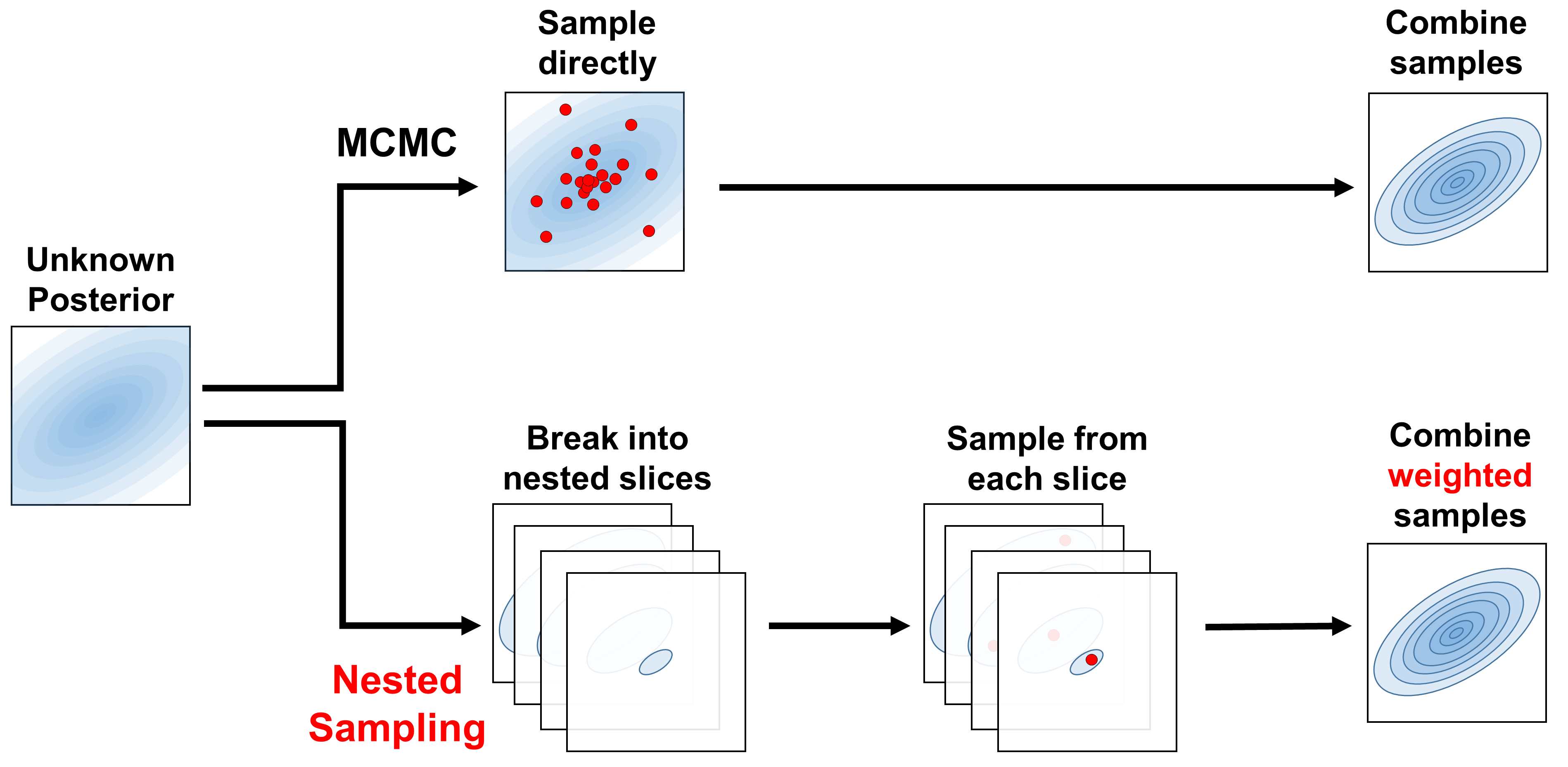
The general motivation for Nested Sampling, first proposed by Skilling (2004) and later fleshed out in Skilling (2006), stems from the fact that sampling from the posterior directly is hard. Methods such as Markov Chain Monte Carlo (MCMC) attempt to tackle this single difficult problem directly. Nested Sampling, however, instead tries to break down this single hard problem into a larger number of simpler problems by:
-
1.
“slicing” the posterior into many simpler distributions,
-
2.
sampling from each of those in turn, and
-
3.
re-combining the results afterwards.
We provide a schematic illustration of this procedure in Figure 1 and give a broad overview of this process below. For additional details, please see Appendix A.
2.1 Overview
Unlike MCMC methods, which attempt to estimate the posterior directly, Nested Sampling instead focuses on estimating the evidence
| (6) |
As this integral is over the entire multi-dimensional domain of , it is traditionally very challenging to estimate.
Nested Sampling approaches this problem by re-factoring this integral as one taken over prior volume of the enclosed parameter space
| (7) |
Here, now defines an iso-likelihood contour (or multiple) defining the edge(s) of the volume , while the prior volume
| (8) |
is the fraction of the prior where the likelihood is above some threshold . Since the prior is normalized, this gives and , which define the bounds of integration for equation (7).
As a rough analogy, we can consider trying to integrate over a spherically-symmetric distribution in 3-D. While it is possible to integrate over directly, it often is significantly easier to instead integrate over differential volume elements as a function of radius :
Parameterizing the evidence integral this way allows Nested Sampling (in theory) to convert from a complicated -dimensional integral over to a simple 1-D integral over .
While it is straightforward to evaluate the likelihood at a given position , estimating the associated prior volume and its differential is substantially more challenging. We can, however, generate noisy estimates of these quantities by employing the procedure described in Algorithm 1. We elaborate further on this procedure and how it works below.
2.2 Generating Samples
A core element of Nested Sampling is the ability to generate samples from the prior subject to a hard likelihood constraint . The most naive algorithm that satisfies this constraint is simple rejection sampling: at a given iteration , generate samples from the prior until .
In practice, however, this simple procedure becomes progressively less efficient as time goes on since the remaining prior volume at each iteration of Algorithm 1 keeps shrinking. We therefore need a way of directly generating samples from the constrained prior:
| (9) |
Sampling from this constrained distribution is difficult for an arbitrary prior since the density can vary drastically from place to place. It is simpler, however, if the prior is standard uniform (i.e. flat from to ) in all dimensions so that the density interior to is constant then behaves more like a typical volume . We can accomplish this through the use of the appropriate “prior transform” function which maps a set of parameters with a uniform prior over the -dimensional unit cube to the parameters of interest .333 In general, there is a uniquely defined prior transform for any given ; see the dynesty documentation for additional details. Taken together, these transform our original hard problem of sampling from the posterior directly to instead the much simpler problem of repeatedly sampling uniformly444Technically this requirement is overly strict, as Nested Sampling can still be valid even if the samples at each iteration are correlated. See Appendix A for additional discussion. within the transformed constrained prior
| (10) |
Throughout the rest of the text we will henceforth assume is a unit cube prior unless otherwise explicitly specified.
Because there is no constraint that this distribution is uni-modal, the constrained prior may define several “blobs” of prior volume that we are interested in sampling from. While sampling from the blob(s) might be hard to do from scratch, because Nested Sampling samples at many different likelihood “levels”, structure tends to emerge over time rather than all at once as we transition away from the prior .
2.3 Estimating the Prior Volume
As shown in Appendix A, generating samples following the strategy in §2.2 based on Algorithm 1 allows us to estimate the (change in) prior volume at a given iteration using the set of “dead” points (i.e. the live points we replaced at each iteration). In particular, it leads to exponential shrinkage such that the (log-)prior volume at each iteration changes by
| (11) |
where is the expectation value (i.e. mean) and we have adopted the notation to emphasize that we have a noisy estimator of the prior volume . Using more live points thus increases our volume resolution by decreasing the rate of this exponential compression. By default, dynesty uses live points, although this should be adjusted depending on the problem at hand.
Once some stopping criterion is reached and sampling terminates after iterations, the remaining set of live points are then distributed uniformly within the final prior volume (see Appendix A). These can be “recycled” into the final set of samples by sequentially adding the live points to the list of “dead” points collected at each iteration in order of increasing likelihood. This leads to uniform shrinkage of the prior volume such that the (fractional) change in prior volume for the th live point added this way is
| (12) |
where is the estimating remaining prior volume at the final th iteration.
2.4 Stopping Criterion
Since Nested Sampling is designed to estimate the evidence, a natural stopping criterion (see, e.g., Skilling, 2006; Keeton, 2011; Higson et al., 2017a) is to terminate sampling when we believe our set of dead points (and optionally the remaining live points) give us an integral that encompasses the vast majority of the posterior. In other words, at a given iteration , we want to terminate sampling if
| (13) |
where is the estimated remaining evidence we have yet to integrate over and determines the tolerance. If the final set of live points are excluded from the set of dead points, dynesty assumes a default value of (i.e. of the evidence remaining). If the final set of live points are included, dynesty instead uses the slightly more permissive .
While the remaining evidence is unknown, we can in theory construct a strict upper bound on it by assigning
| (14) |
where is the maximum-likelihood value across the entire domain and is the prior volume at the current iteration. This is equivalent to treating the remaining likelihood interior to the current sample () as a uniform slab with amplitude .
Unfortunately, neither or is known exactly. However, we can approximate this upper bound by replacing both quantities with associated estimators to get the rough upper bound
| (15) |
where is the maximum value of the likelihood among the live points at iteration and is the estimated (remaining) prior volume.
While this rough upper bound works well in most cases, because we only have access to the best likelihood sampled by the live points at a particular iteration there is always a chance that and that we will terminate early. This can happen if there is an extremely narrow likelihood peak within the remaining prior volume that has not yet been discovered by the live points.
2.5 Estimating the Evidence and Posterior
Once we have a final set of samples , we can estimate the 1-D evidence integral using standard numerical techniques. To ensure approximation errors on the numerical integration estimate are sufficiently small, dynesty uses the 2nd-order trapezoid rule
| (16) |
where and
| (17) |
is the estimated importance weight. By default, dynesty uses the mean values of to compute the mean and standard deviation of following Appendix A, although these values can also be simulated explicitly.
We can also estimate the posterior from the same set of dead points by using the associated importance weights derived above:
| (18) |
By default, dynesty uses the mean values of to compute this posterior estimate, although as with the evidence these values can also be simulated explicitly (see Appendix A).
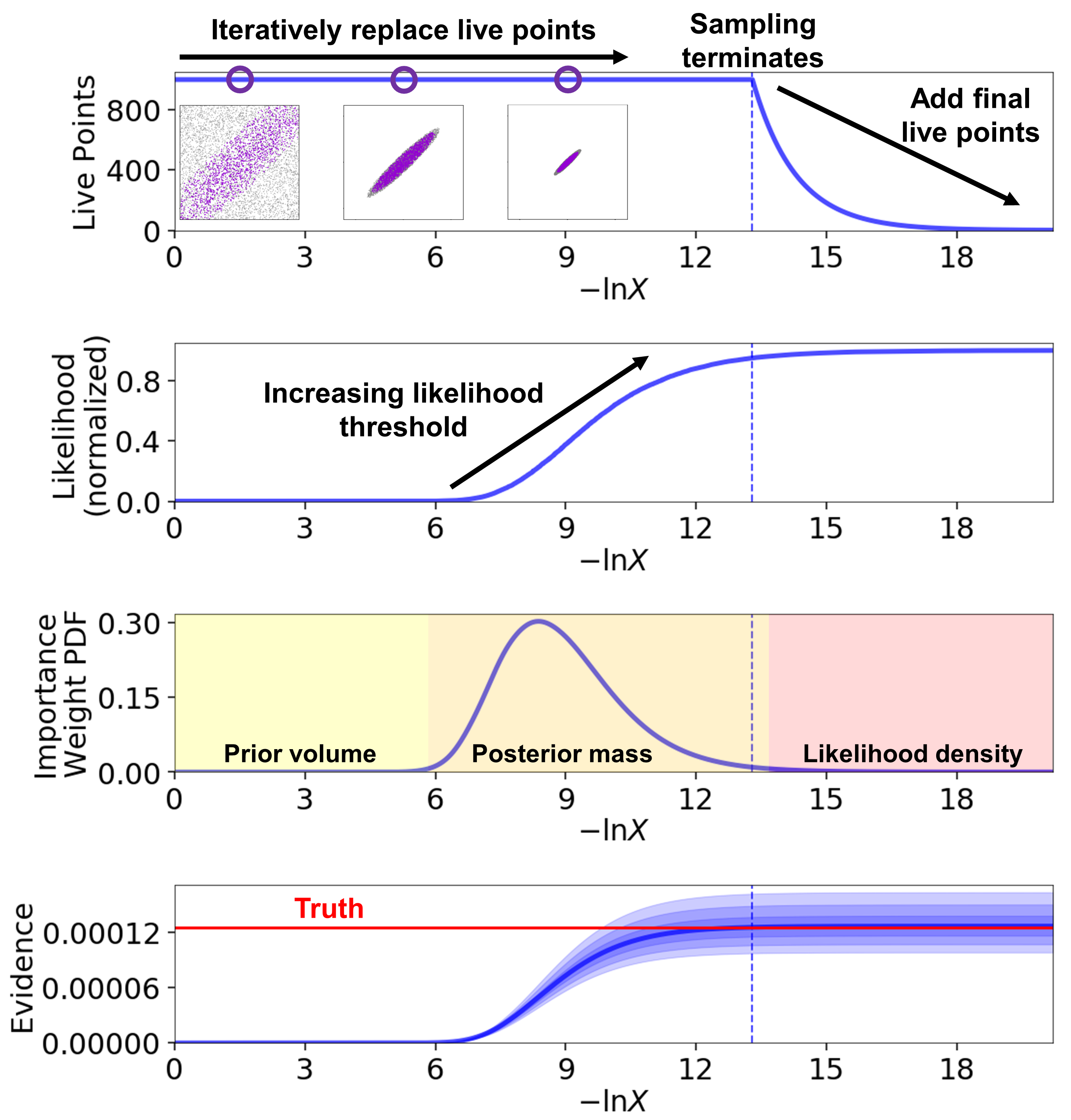
An illustration of a typical Nested Sampling run is shown in Figure 2.
2.6 Benefits of Nested Sampling
Because of its alternative approach to sampling from the posterior, Nested Sampling has a number of benefits relative to traditional MCMC approaches:
- 1.
-
2.
Nested sampling can sample from multi-modal distributions that tend to challenge many MCMC methods.
-
3.
While most MCMC stopping criteria based on effective sample sizes can feel arbitrary, Nested Sampling possesses well-motivated stopping criteria focused on evidence estimation.
-
4.
MCMC methods need to converge (i.e. “burn in”) to the posterior before any samples generated are valid. While optimization techniques can speed up this process, assessing this convergence can be challenging and time-consuming (Gelman & Rubin, 1992; Vehtari et al., 2019). Nested Sampling doesn’t suffer from similar issues because the method smoothly integrates over the posterior starting from the prior .
2.7 Drawbacks
While Nested Sampling has its fair share of benefits that have encouraged its rapid adoption in astronomical Bayesian analyses, it also suffers from a fair share of drawbacks. Most crucially, the standard Nested Sampling implementation outlined in Algorithm 1 focuses exclusively on estimating the evidence ; the posterior is entirely a by-product of the approach. This creates several immediate drawbacks relative to MCMC, which focuses exclusively on sampling the posterior .
First, because most Nested Sampling implementations rely on sampling from uniform distributions (see §2.2), applying them to general distributions requires knowing the appropriate prior transform . While these are straightforward to define when the prior can be decomposed into separable, independent components, they can be more difficult to derive when the prior involves conditional and/or jointly distributed parameters.
Second, because the evidence depends on the amount of prior volume that needs to be integrated over, the overall expected runtime is sensitive to the relative size of the prior. In other words, while estimating the posterior mostly depends on generating samples close to where the majority of the distribution is located (i.e. the “typical set”; Betancourt, 2017), estimating the evidence requires generating samples in the extended tails of the distribution. Using less informative (broader) priors will increase the expected runtime even if the posterior is largely unchanged.
Finally, because the number of live points is constant, the rate at which we integrate over the posterior is the same regardless of where we are. This means that increasing the number of like points , which increases the overall runtime, always improves the accuracy of both the posterior and evidence estimates. In other words, Nested Sampling does not allow users to prioritize between estimating the posterior or the evidence, which is not ideal for many analyses that are mostly interested in using Nested Sampling for either option. We focus on improving this behavior in §3.
As with any sampling method, we strongly advocate that Nested Sampling should not be viewed as being strictly “better” or “worse” than MCMC, but rather as a tool that can be more or less useful in certain problems. There is no “One True Method to Rule Them All”, even though it can be tempting to look for one.
3 Dynamic Nested Sampling
In our overview of Nested Sampling in §2, we highlighted three main drawbacks of basic implementations:
-
1.
They generally require a prior transform.
-
2.
Their runtime is sensitive to the size of the prior.
-
3.
Their rate of posterior integration is always constant.
While the first two drawbacks are essentially inherent to Nested Sampling as sampling strategy, the last is not. Instead, the inability of Algorithm 1 to “prioritize” estimating the evidence or posterior is a consequence of the fact that the number of live points remains constant throughout an entire run, which sets the rate of integration . As a result, we will henceforth call this procedure “Static” Nested Sampling.
To address this issue, Higson et al. (2017b) proposed a deceptively simple modification: let the number of live points vary during runtime. This gives a new “Dynamic” Nested Sampling algorithm whose basic implementation is outlined in Algorithm 2. This simple change is transformative, allowing Dynamic Nested Sampling to focus on sampling the posterior , similar to MCMC approaches, while retaining all the benefits of (Static) Nested Sampling to estimate the evidence and sample from complex, multi-modal distributions. It also possesses well-motivated new stopping criteria for posterior and evidence estimation.
It is important to note that we cannot take advantage of the flexibility offered by Dynamic Nested Sampling, however, without implementing appropriate schemes to specify exactly how live points should be allocated, when to terminate sampling, etc. While dynesty tries to implement a number of reasonable default choices, in practice this inevitably leads to many more tuning parameters that can affect the behavior of a given Dynamic Nested Sampling run.
We provide an illustration of the overall approach in Figure 3 and give a broad overview of the basic algorithm below. For additional details, please see Appendix A.
3.1 Allocating Live Points
The singular defining feature of the Dynamic Nested Sampling algorithm is the scheme we use for determining how the number of live points at a given iteration should vary. Naively, we would like to be larger where we want our resolution to be higher (i.e. a slower rate of integration ) and smaller where we are interested in traversing the current region of prior volume more quickly. This allows us to prioritize adding samples in regions of interest.
In general, we would like the number of live points as a function of prior volume to follow a particular importance function such that
| (19) |
While this function can be completely general, since most users are interested in estimating the posterior and/or evidence more generally, dynesty by default follows Higson et al. (2017b) and considers a function of the form:
| (20) |
where is the relative amount of importance placed on estimating the posterior.
We define the posterior importance function as
| (21) |
where is the now the probability density function (PDF) of the importance weight defined in §2.5. This choice just means that we want to allocate more live points in regions where the posterior mass is higher.
We define the evidence importance function as
| (22) |
where is the evidence integrated up to . This means that we want to allocate more live points when we believe we have not integrated over much of the posterior (i.e. in the prior volume-dominated regime at larger values of ) and fewer as we integrate over larger portions of the posterior mass and become more confident in our estimated value of (see Figure 2).
3.2 Iterative Dynamic Nested Sampling
As in §2.4, we unfortunately do not have access to or directly. We thus need to use noisy estimators to approximate them, which are only available after we have already generated samples from the posterior. In practice then, Dynamic Nested Sampling works as an iterative modification to Static Nested Sampling. We outline this “Iterative” Dynamic Nested Sampling approach, first proposed in Higson et al. (2017b) and implemented in dynesty, in Algorithm 3. It has five main steps:
-
1.
Sample the distribution with Static Nested Sampling to lay down a “baseline run” to get a sense where the posterior mass is located.
-
2.
Evaluate our importance function over the existing set of samples.
-
3.
Use the computed importances to decide where to allocate additional live points/samples.
-
4.
Add a new “batch” of samples in the region of interest using Static Nested Sampling.
-
5.
“Merge” the new batch of samples into the previous set of samples.
We then repeat steps (ii) to (v) until some stopping criterion is met. By default, dynesty uses points for each run, although this should be adjusted depending on the problem at hand.
Allocating points using an existing set of samples is a two-step process. First, we evaluate a noisy estimate of our importance function over the samples:
| (23) |
where we are now using the noisy importance weight to estimate the posterior and the rough upper limit to estimate the remaining evidence. Then, we use these values to define new regions of prior volume to sample. By default, dynesty only samples from a single contiguous range of prior volume which define an associated (flipped) range in iteration and likelihood defined by the simple heuristic
| (24) | ||||
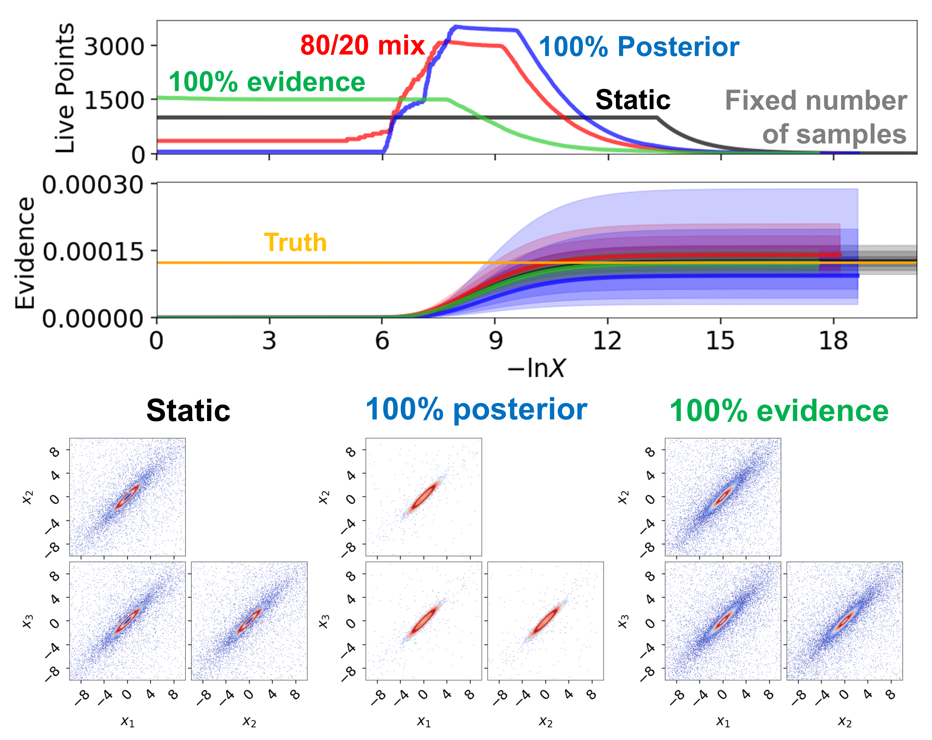
where serves as a threshold relative to the peak value and pads the starting/ending iteration. In other words, we compute the importance values over the existing set of samples, compute the minimum and maximum iterations where the importance is above a threshold relative to the peak, and shift the final values by . By default, dynesty assumes (80% posterior vs 20% evidence), (80% thresholding), and .
Once we have computed , we can then just start a new Static Nested Sampling run that samples from the constrained prior between . In the case where , this is just the original prior and our Static Nested Sampling run is identical to Algorithm 1 except with stopping criteria . If , however, then we are instead starting interior to the prior and thus not fully integrating over it. So while those new samples will improve the relative posterior resolution and thus the posterior estimate , they will not actually improve the evidence estimate .
Finally, we need to “merge” our new set of samples into our original set of samples . This process is straightforward and can be accomplished following the procedure outlined in Appendix A. We are then left with a combined set of samples with new associated prior volumes and a variable number of live points at every iteration.
3.3 Estimating the Prior Volume
As shown in Appendix A, we can reinterpret the results from §2.3 as a consequence of the two different ways Nested Sampling traverses the prior volume. In the first case, where the number of live points increases or stays the same, we know that we have (possibly) added live points and then replaced the one with the lowest likelihood . In this case, the prior volume experiences exponential shrinkage such that
| (25) |
In the second case, where the number of live points strictly decreases, we know that we have removed the live point(s) with the lowest likelihood . For each of the iterations where this continues to occur, the prior volume experiences uniform shrinkage such that
| (26) |
In Static Nested Sampling, these two regimes are cleanly divided, with the main set of dead points traversing the prior volume exponentially and the final set of “recycled” live points traversing it uniformly. In Dynamic Nested Sampling, however, we are constantly switching between exponential and uniform shrinkage as we increase or decrease the number of live points at a given iteration.
3.4 Stopping Criterion
The implementation of Static Nested Sampling outlined in Algorithm 1 generally exclusively targets evidence estimation. This gives a natural stopping criterion (see §2.4) to terminate sampling once we believe that we have integrated over a majority of the posterior such that additional samples will no longer improve our evidence estimate .
In the Dynamic Nested Sampling case, however, we are no longer just interested in computing the evidence. Because we now have the flexibility to vary the number of live points over time, we are also interested in the properties of our integral (and the samples that comprise the integrand) in addition to the question of whether our integral has converged.
This flexibility necessitates the introduction of more complex stopping criteria to assess whether those alternative properties are behaving as expected. Similar to §3.1, we consider a stopping criteria of the form:
| (27) |
where is our tolerance, is the posterior stopping criterion, is the evidence stopping criterion, and is the relative amount of weight given to over .
We define our stopping criterion to be the amount of fractional uncertainty in the current posterior and evidence estimates. For the posterior , we start by defining “posterior noise” to be the Kullback-Leibler (KL) divergence
| (28) | |||
| (29) |
between the posterior estimate from a random hypothetical Nested Sampling run with the same setup and our current estimate . This can be interpreted as the “information loss” due to random noise in our posterior estimate . Our proposed posterior stopping criteria is then
| (30) |
where normalizes the posterior deviation to a desired scale. For the evidence , this is just the estimated fractional scatter between the evidence estimates from random hypothetical Nested Sampling runs with the same setup. Following Higson et al. (2017b), we opt to compute this in log-space for convenience:
| (31) |
where normalizes the evidence deviation to a desired scale.
Unsurprisingly, we do not have access to the distribution of all hypothetical Nested Sampling runs with the same setup to compute these exact estimates. However, as with §2.4 and §3.2, we do have access to noisy estimates of these quantities via procedures described in Higson et al. (2017a) and outlined in Appendix A for simulating Nested Sampling errors. dynesty uses simulated values of these noisy estimates to estimate the stopping criteria as:
| (32) |
where the notation just emphasizes that we are constructing a noisy estimator of our already-noisy estimate . By default, dynesty assumes (100% focused on reducing posterior noise), , , , and .
4 Implementation
Now that we have outlined the basic algorithm and approach behind Dynamic Nested Sampling, we now turn our attention to the problem of generating samples from the constrained prior. dynesty approaches this problem in two parts:
-
1.
constructing appropriate bounding distributions that encompass the remaining prior volume over multiple possible modes and
-
2.
proposing new live points by generating samples conditioned on these bounds.
dynesty contains several options for both constructing bounds and sampling conditioned on them. We provide an broad overview of each of these in turn.
4.1 Bounding Distributions
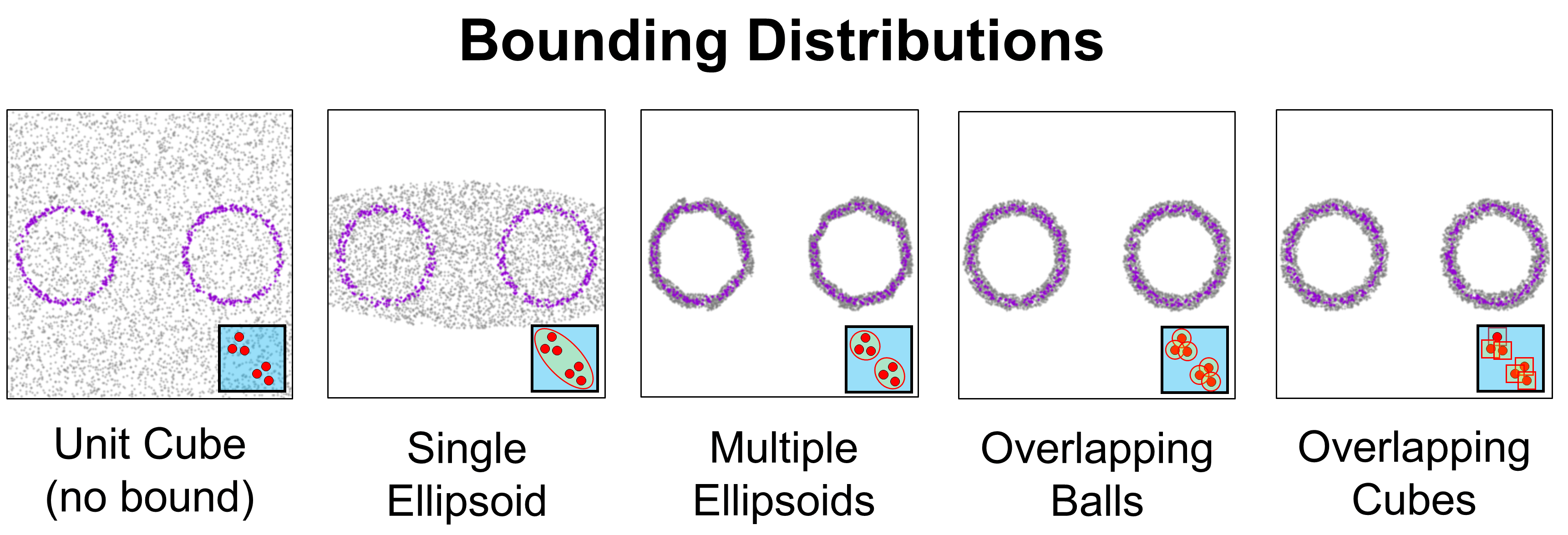
In general, dynesty tries to use the distribution of the current set of live points to try and get a rough idea of the shape and size of the various regions of prior volume that we are currently sampling. These are then used to condition various sampling methods to try and improve the efficiency. There are five bounding methods currently implemented in dynesty:
-
•
no bounds (i.e. the unit cube),
-
•
a single ellipsoid,
-
•
multiple ellipsoids,
-
•
many overlapping balls, and
-
•
many overlapping cubes.
In general, single ellipsoids tend to perform reasonably well at estimating structure when the likelihood is roughly Gaussian and uni-modal. In more complex cases, however, decomposing the live points into separate clusters with their own bounding ellipsoids works reasonably well at locating and tracking structure. In low () dimensions, allowing the live points themselves to define emergent structure through many overlapping balls or cubes can perform better provided the spans similar scales in each of the parameters. Finally, using no bounds at all is only recommended as an option of last resort and is mostly relevant when performing systematics checks or if the number of live points is small relative to the number of possible parameter covariances.
In addition to these various options, dynesty also tries to increase the volume of all bounds by a factor to be conservative about the size of the constrained prior. While this is generally assumed to take a constant value of , it can also be derived “on the fly” using bootstrapping methods following the approach outlined in Buchner (2016). Deriving accurate volume expansion factors are extremely important when sampling uniformly but are less relevant for other sampling schemes that are more robust to the exact sizes of the bounds (see §4.2).
By default, dynesty uses multiple ellipsoids to construct the bounding distribution. A summary of the various bounding methods can be found in Figure 4. We describe these each in turn below.
4.1.1 Unit Cube
The simplest case of using the entire unit cube (i.e. simple rejection sampling over the entire prior with no limits) can be useful in a few edge cases where the number of live points is small compared to the number of dimensions , or where users are interested in performing tests to verify sampling behavior.
4.1.2 Single Ellipsoid
As shown in (Mukherjee et al., 2006), a single bounding ellipsoid can be effective if the posterior is unimodal and roughly Gaussian. dynesty uses a scaled version of the empirical covariance matrix centered on the empirical mean of the current set of live points to determine the size and shape of the ellipsoid, where is set so the ellipsoid encompasses all available live points.
4.1.3 Multiple Ellipsoids
By default, dynesty does not assume the posterior is unimodal or Gaussian and instead tries to bound the live points using a set of (possibly overlapping) ellipsoids. These are constructed using an iterative clustering scheme following the algorithm outlined in Shaw et al. (2007) and Feroz & Hobson (2008) and implemented in the online package nestle.555 dynesty is built off of nestle with the permission of its developer Kyle Barbary. In brief, we start by constructing a bounding ellipsoid over the entire collection of live points. We then initialize 2 -means clusters at the endpoints of the major axes, optimize their positions, assign live points to each cluster, and construct a new pair of bounding ellipsoids for each new cluster of live points. The decomposition is accepted if the combined volume of the subsequent pair of ellipsoids is substantially smaller. This process is then performed recursively until no decomposition is accepted.
By default, dynesty tries to be substantially more conservative when decomposing live points into separate clusters and bounding ellipsoids than alternative approaches used in MultiNest (Feroz & Hobson, 2008; Feroz et al., 2013). This algorithmic choice, which can substantially reduce the overall sampling efficiency, is made in order to avoid “shredding” the posterior into many tiny islands of isolated live point clusters. As shown in Buchner (2016), that behavior can lead to biases in the estimated evidence and posterior .
4.1.4 Overlapping Balls
An alternate approach to using bounding ellipsoids is to allow the current set of live points themselves to define emergent structure. The simplest approach used in dynesty follows Buchner (2016, 2017) by assigning a -dimensional ball (sphere) with radius to each live point, where is set using bootstrapping and/or leave-one-out techniques to encompass other live points. One benefit to this approach over using multiple ellipsoids (which can depend sensitively on the clustering schemes) is that it is almost entirely free of tuning parameters, with the overall behavior only weakly dependent on the number of bootstrap realizations.
4.1.5 Overlapping Cubes
4.2 Sampling Methods
Once a bounding distribution has been constructed, dynesty generates samples conditioned on those bounds. In general, this follows a strategy of
| (33) |
where is the covariance associated with a particular bound (e.g., an ellipsoid), is the starting position, is the final proposed position, and is a scale-factor that is adaptively tuned over the course of a run to ensure optimal acceptance rates.
dynesty implements four main approaches to generating samples:
-
•
uniform sampling,
-
•
random walks,
-
•
multivariate slice sampling, and
-
•
Hamiltonian slice sampling.
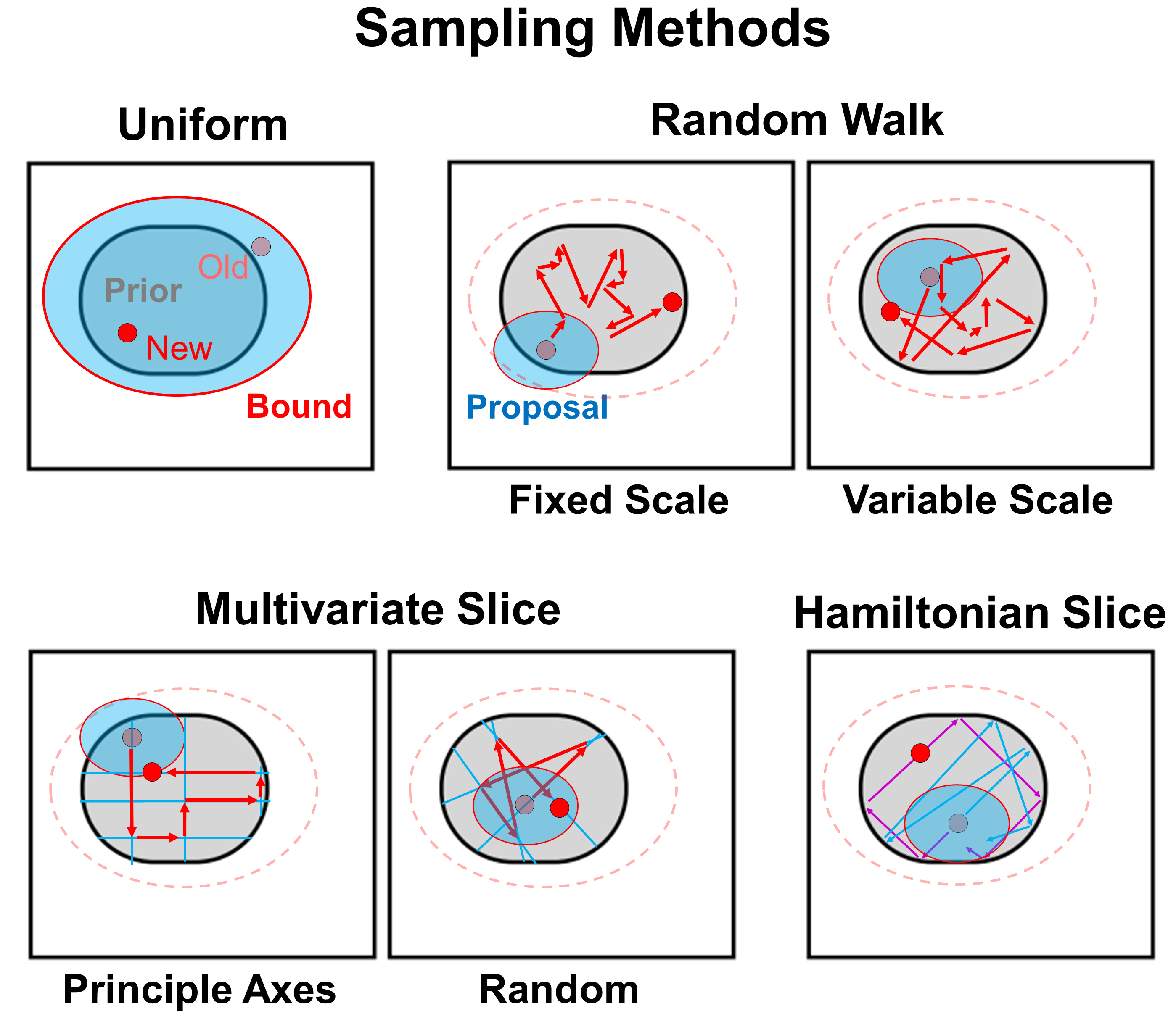
These each are designed for different regimes. Uniform sampling can be relatively efficient in lower dimensions where the bounding distribution can approximate the prior volume better but struggles in higher dimensions since it is extremely sensitive to the size of the bounds. Random walks are less sensitive to the size of the bounding distribution and so tend to work better than uniform sampling in moderate dimensional spaces but still struggle in high-dimensional spaces because of the exponentially increasing amount of volume it needs to explore. Multivariate and Hamiltonain slice sampling often performs better in these high-dimensional regimes by avoiding sampling directly from the volume and taking advantage of gradients, respectively.
In addition to each method’s performance in various regimes, there is also a fundamental qualitative difference between uniform sampling and the other sampling approaches outlined above. Uniform sampling, by construction, can only sample directly from the bounding distribution. This makes it uniquely sensitive to the assumption that the bounds entirely encompass the current prior volume at a given iteration, which is never fully guaranteed (Buchner, 2016). By contrast, the other sampling methods are MCMC-based: they generate samples by “evolving” a current live point to a new position. This allows them to generate samples outside the bounding distribution, making them less sensitive to this assumption.
By default, dynesty resorts to uniform sampling when the number of dimensions , random walks when , and Hamiltonian/multivariate slice sampling when if a gradient is/is not provided. A summary of the various sampling methods can be found in Figure 5. We describe these each in turn below.
4.2.1 Uniform Sampling
If we assume that our bounding distribution encloses the constrained prior , the most direct approach to generating samples from the bounds is to sample from them uniformly. This procedure by construction produces entirely independent samples between each iteration , and tends to work best when the volume of the bounds is roughly the same order of magnitude as the current prior volume (leading to acceptance rates).
In general, the procedure for generating uniform samples from overlapping bounds is straightforward (see, e.g., Feroz & Hobson, 2008; Buchner, 2016):
-
1.
Pick a bound at random with probability proportional to its volume .
-
2.
Sample a point uniformly from the bound.
-
3.
Accept the point with probability , where is the number of bounds lies within.
This approach ensures that any proposed sample will be drawn from the bounding distributing comprised of the union of all bounds, which has a volume that is strictly less than or equal to the sum of the volumes of each individual bound.
Generating samples uniformly from the bounds in §4.1 falls into two cases: cubes and ellipsoids. Generating points from an -cube centered at with half-side-length is trivial and can be accomplished via:
-
1.
Generate iid uniform random numbers from .
-
2.
Set .
Generating points from an ellipsoid centered at with covariance with matrix square-root is also straightforward but slightly more involved:
-
1.
Generate iid standard normal random numbers .
-
2.
Compute the normalized vector .
-
3.
Draw a standard uniform random number and compute .
-
4.
Set .
Step (ii) creates a random vector that is uniformly distributed on the surface of the -sphere. Step (iii) randomly moves to an interior radius based on the fact that the volume of a -sphere scales as . Finally, step (iv) adjusts the scale, shape, and center to match that of the bounding ellipsoid.
4.2.2 Random Walks
An alternative approach to sampling uniformly within the bounding distribution is to instead to try and propose new positions by “evolving” a given live point to a new position. Since at a given iteration by definition, this procedure also guarantees that we will be generating samples exclusively within the constrained prior .
One straightforward approach to “evolving” a live point to a new position is to consider sampling from the constrained prior using a simple Metroplis-Hastings (MH; Metropolis et al., 1953; Hastings, 1970) MCMC algorithm:
-
1.
Propose a new position from the proposal distribution starting from .
-
2.
Move to with probability . Otherwise, stay at .
-
3.
Repeat (i)-(ii) for iterations.
Since the constrained prior is flat (see §2.2), the ratio of the constrained prior values is by definition . Likewise, if we choose a symmetric proposal distribution , then the ratio of the proposal distributions also evaluates to . This procedure then reduces to simply accepting a new point if it is within the constrained prior with and rejecting it otherwise. By default, dynesty takes .
dynesty implements two forms of the proposal . The default option is to propose new positions uniformly from an associated ellipsoid centered on with covariance , where is one of the bounding distributions that encompasses (selected randomly). The second follows the same form as the first, except the covariance is re-scaled at each subsequent proposal by following the procedure outlined in Sivia & Skilling (2006):
| (34) |
where and is the total number of accepted and rejected proposals by iteration , respectively, is the desired acceptance fraction, and . By default, dynesty targets .
4.2.3 Multivariate Slice Sampling
In higher dimensions, rejection sampling-based methods such as the random walk proposals outlined in §4.2.2 can become progressively more inefficient. To remedy this, dynesty includes slice sampling (Neal, 2003) routines designed to sample from the constrained prior . These are based on the “stepping out” method proposed in Neal (2003) and Jasa & Xiang (2012), which works as follows in the single-variable case starting from the position of the th live point:
-
1.
Draw a standard uniform random number .
-
2.
Set the left bound and the right as where is the starting “window”.
-
3.
While , extend the position of the left bound by . Repeat this procedure for .
-
4.
Sample a point uniformly on the interval from to .
-
5.
If , accept . Otherwise, reassign the corresponding bound to be ( if and otherwise) and repeat steps (iv)-(v).
When sampling in higher dimensions, the single-variable update outlined above can be interpreted as a Gibbs sampling update (Geman & Geman, 1987) where instead of drawing directly we instead update each component in turn
| (35) |
where are the set of parameters excluding . We then repeat this procedure for iterations. By default dynesty takes .
This procedure is generally robust, although it can introduce longer correlation times if there are strong covariances between parameters. To mitigate this, dynesty by default executes single-variable slice sampling updates along the principle axes associated with the covariance from a given bound . This allows us to automatically set both the direction and associated scale of the window while trying to reduce the correlations among sets of parameters.
Alternately, instead of executing a full Gibbs update by rotating through the entire set of parameters in turn, we can sample along a random trajectory through the prior instead. This procedure is similar to that implemented in PolyChord (Handley et al., 2015), except that rather than “whitening” the set of live points using the associated we instead draw from the surface of the corresponding bound with covariance . Provided a suitable number of , this procedure also can generate suitably independent new positions .
4.2.4 Hamiltonian Slice Sampling
Over the past two decades, sampling methods have increasingly attempted to incorporate gradients to improve their overall performance, especially in high-dimensional spaces. The most common class of methods are based on Hamiltonian Monte Carlo (HMC; Neal, 2012; Betancourt, 2017), whereby a particle at a given position is assigned a mass matrix and some momentum and allowed to sample from the joint distribution
| (36) |
where
| (37) |
is the Hamiltonian of the system with a “potential energy” and “kinetic energy” , and is the transpose operator. Typically, proposals are generated by sampling the momentum from the corresponding multivariate Normal (Gaussian) distribution
| (38) |
with mean and covariance , evolving the system via Hamilton’s equations from , and then accepting the new position based on the MH acceptance criteria outlined in §4.2.2. In other words, at each iteration we randomly assign a given particle some mass and velocity and then have it explore the potential defined by the (log-)posterior.
As with the previous methods, this approach simplifies dramatically when sampling over the constrained prior . In that case, since the distribution is flat, the momentum remains unchanged until the particle hits the hard likelihood boundary, at which point it reflects so that
| (39) |
where is the gradient at the point of reflection. This version of the algorithm is referred to elsewhere as Galilean Monte Carlo (Skilling, 2012; Feroz & Skilling, 2013) or reflective slice sampling (Neal, 2003).
In practice, since we have to evolve the system discretely, there are a few additional caveats to consider. Most importantly, the use of discrete time-steps means reflection will not occur right at the boundary of the constrained prior but slightly beyond it, which does not guarantee reflections will end up back inside the constrained prior. This behavior, which arises from larger time-steps, “terminates” the particle’s trajectory in that particular direction and leads to inefficient sampling that isn’t able to explore the full parameter space.
On the other hand, using extremely small time-steps means spending the vast majority of time evaluating positions along a straight line, which is also non-optimal. dynesty by default attempts to compromise between these two behaviors by optimizing the time-step so that of total steps are spent moving forward passively instead of reflecting or terminating. In addition, dynesty by default caps the total number of time-steps to to prevent trajectories from being evolved indefinitely.
Similar to algorithms such as the No U-Turn Sampler (NUTS; Hoffman & Gelman, 2011), dynesty also considers trajectories evolved forwards and backwards in time to broaden the range of possible positions explored in a given proposal. While these roughly double the number of overall time-steps, they substantially improve overall behavior by exploring larger regions of the constrained prior.
dynesty employs two additional schemes to try and further mitigate discretization effects on the sampling procedure described above. First, the time-step used at a given iteration is allowed to vary randomly by up to following recommendations from Neal (2012). This helps to suppress resonant behavior that can arise from poor choices of time-steps without substantially impacting overall performance. Second, rather than merely accepting positions at the end of a trajectory, dynesty instead tries to sample uniformly from the entire trajectory by treating it as a set of slices defined by left-inner-right position tuples. New samples are then proposed via the following scheme:
-
1.
Compute the length of each line segment .
-
2.
Selecting a line segment at random proportional to its length.
-
3.
Sample a point uniformly on the line segment defined by .
-
4.
If , accept . Otherwise, reassign the corresponding bound to be ( if is on the line segment and otherwise) and repeat steps (i)-(iv).
While there are a variety of possible approaches to applying HMC-like methods to Nested Sampling other than the basic procedure outlined above, we defer any detailed comparisons between them to possible future work.
5 Tests
Here, we examine dynesty’s performance on a variety of toy problems designed to stress-test various aspects of the code. Additional tests can also be found online.
5.1 Gaussian Shells
One standard problem that tests the efficiency of the ability of bounding distributions to transition between a flat surface to separated, elongated structures is the -dimensional “Gaussian shells” from Feroz & Hobson (2008). The likelihood of the distribution is defined as
| (40) |
where
| (41) |
Following Feroz et al. (2013), we take the centers and of the two positions to be and in the first dimension and in all others, respectively, the radius , and the width . Our prior is defined to be uniform from to encompass the majority of the likelihood and ensure a smooth transition between the uni-modal starting distribution and the multi-modal target distribution.
We illustrate dynesty’s performance in the 2-D case in Figure 6. The default configuration options in dynesty (multiple ellipsoid bounds with uniform sampling) lead to a roughly sampling efficiency over the course of k iterations when using Dynamic Nested Sampling and lead to excellent posterior estimates. We also see that the multi-ellipsoidal decomposition algorithm works as expected, with the total volume of the bounding distribution decreasing dramatically as the live points begin to organize themselves within the two shells.
5.2 Eggbox
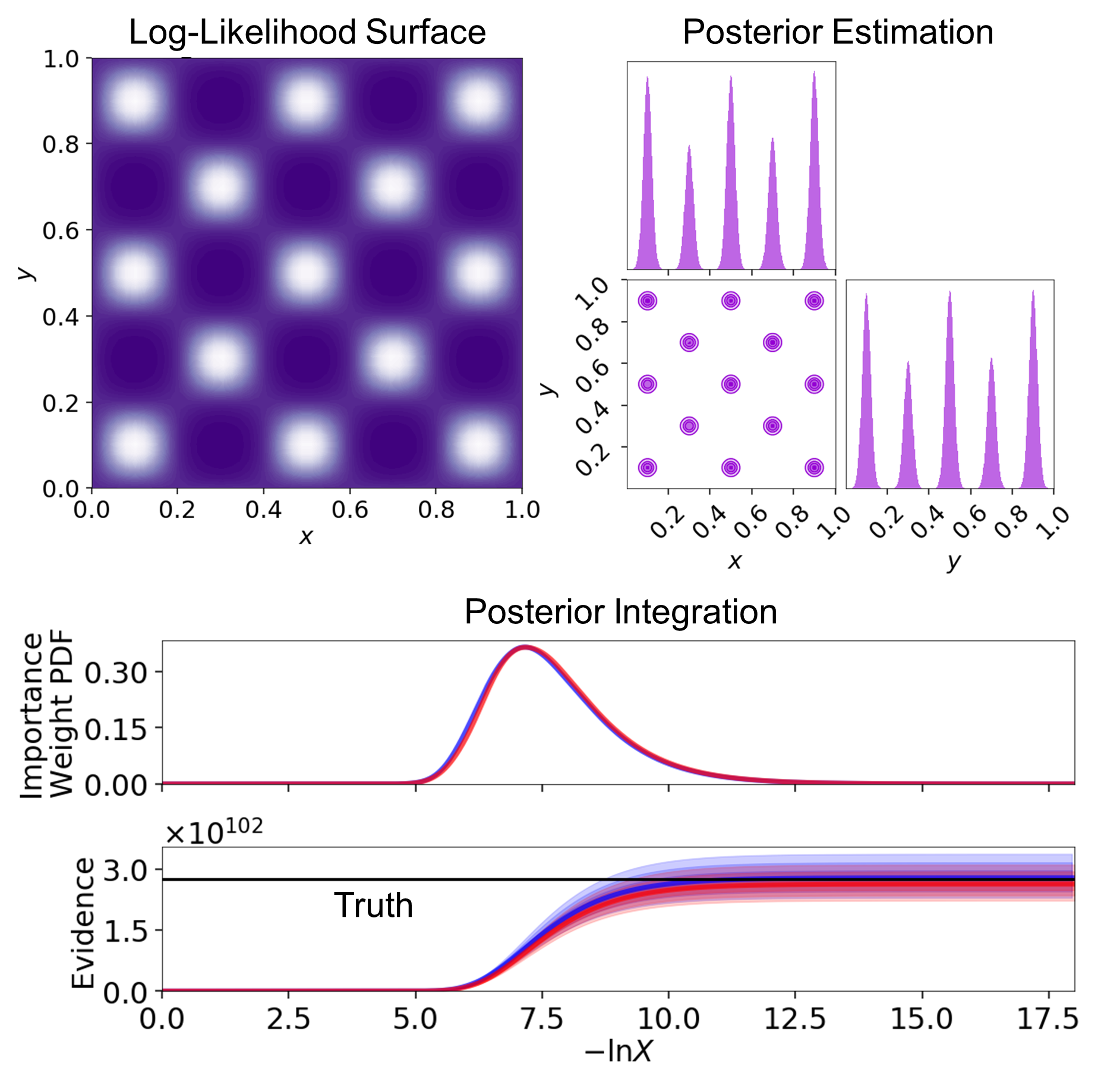
Another distribution we consider to test the ability of dynesty to track and evolve multiple modes is the 2-D “Eggbox” likelihood from Feroz & Hobson (2008), which we defined as
| (42) |
This distribution is periodic over the 2-D unit cube, with 13 localized modes contained within a given period. We take our prior to be standard uniform in and to limit sampling to one period.
The resulting posterior and evidence estimates from several posterior-oriented and evidence-oriented Dynamic Nested Sampling runs are shown in Figure 7. dynesty is able to sample from this distribution quite effectively, with average sampling efficiencies ranging from when sampling uniformly from the multiple ellipsoids or overlapping balls.
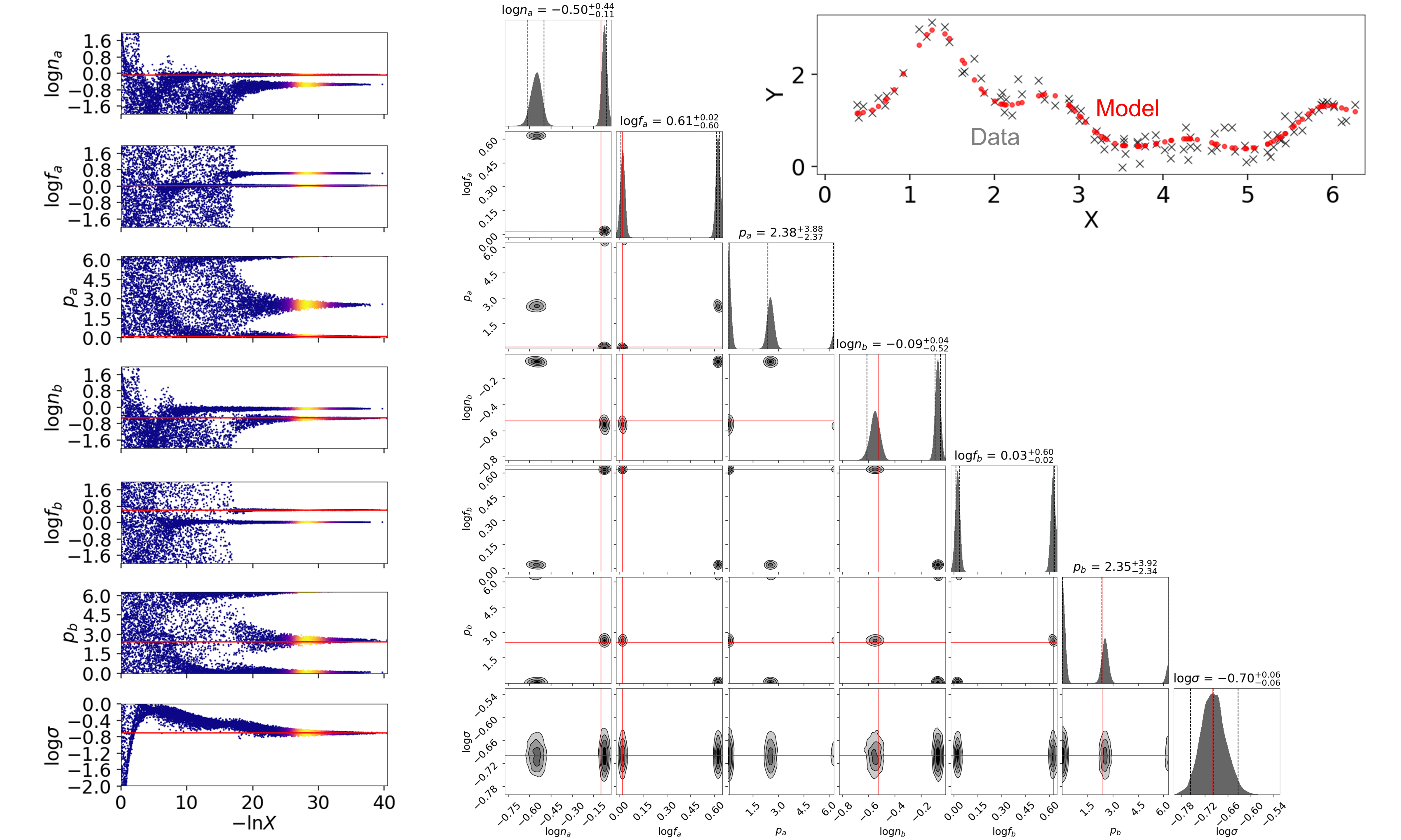
5.3 Exponential Wave
We next apply dynesty to a signal reconstruction problem with multiple modes and periodic boundary conditions. Our model is a transformed periodic single from to :
| (43) |
where we observe noisy data points drawn from
| (44) |
The likelihood for this model is Gaussian over the corresponding observed datapoints such that
| (45) |
and has seven free parameters: two controlling the relevant amplitudes (, ), two controlling the frequencies (, ), two controlling the phases (, ), and one controlling the scatter .
We take our true model parameters to be , , , , , , and so that a solution is close to the boundary. We assign our prior to be uniform or log-uniform in all parameters with , , , , , , and , where the priors in and are periodic.
We illustrate dynesty’s performance on this problem in Figure 8. We find dynesty is able to robustly recover both modes in this problem, including the solution near the boundary.
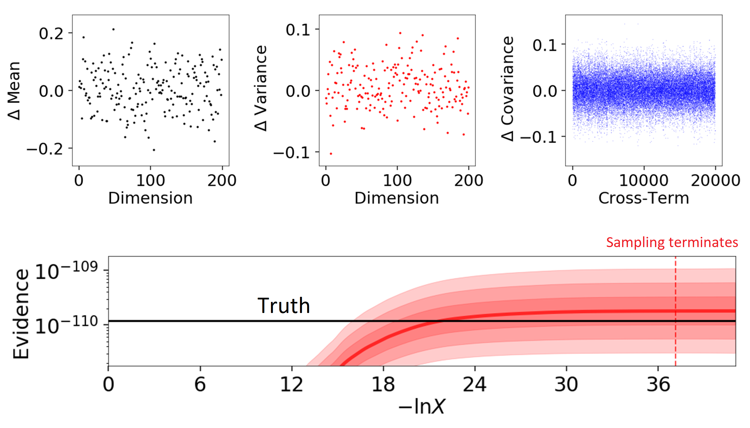
5.4 200-D Gaussian
We next examine dynesty’s behavior in higher dimensions by testing its performance on a 200-D multivariate Gaussian likelihood with mean and covariance where is the identity matrix. We assign an identical prior (iid Gaussian with and ), such that the posterior will also be iid Gaussian with mean but with covariance .
We sample from this distribution using Hamiltonian Slice Sampling with the analytic log-likelihood gradient. To further highlight the efficiency of these proposals to explore the posterior, we use a small () number of live points so that we are highly undersampled relative to the 200-D space. Since dynesty by default uses the empirical covariance (i.e. the MLE estimate) to construct any bounding ellipsoids, this process is dominated by shot noise that can substantially affect the covariance. We consequently impose no bounding distribution (which happens to also be optimal for this problem).
As shown in Figure 9, we find dynesty is able to achieve unbiased recovery of the mean, covariance, and evidence under these conditions. The typical sampling efficiency we achieve for this problem is roughly (i.e. 1000 likelihood calls per iteration), which translates to roughly 5 per dimension.
5.5 Comparison to MCMC
Nested Sampling and MCMC sampling are different tools designed for different types of problems. Here we perform a limited comparison to highlight the advantages/disadvantages of each methodology.
We consider a simple linear regression problem where our model is
| (46) |
and we observe noisy data from
| (47) |
where is the measured variance and corresponds to an additional fractional systematic uncertainty that we would like to infer in addition to and . The likelihood is again Gaussian:
| (48) |
This problem is unimodal and only has three parameters, making it very tractable to both Nested Sampling and MCMC methods.
We choose our priors to be uniform so that , , and , which are substantially broader than the likelihood distribution but not so broad that the runtime of dynesty will be dominated merely integrating over the prior.
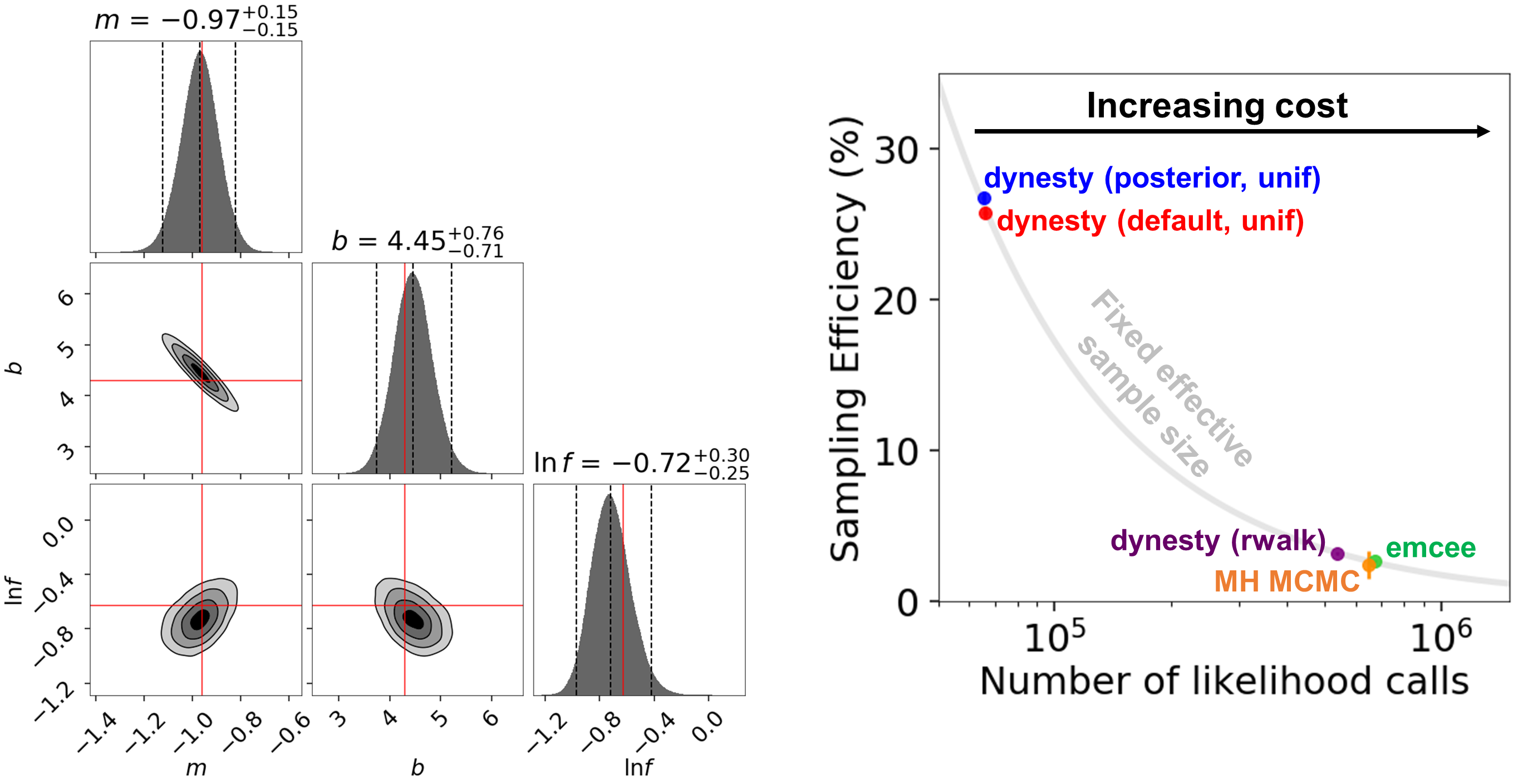
We run dynesty in three configurations to sample from this posterior distribution, using the default settings whenever possible to highlight performance in a “typical” use case. First, we set the weight function to give the posterior 100% of the importance when allocating live points in order to imitate MCMC-like behavior. Then, we revert to the default 80%/20% posterior/evidence weighting scheme to see how much our posterior estimate degrades as we spend a larger fraction of runtime trying to improve our evidence estimates. Finally, we switch out the default sampling mode (uniform sampling) for random walks to forcibly decrease the overall sampling efficiency.
We compare these results to two MCMC alternatives. The first is emcee (Foreman-Mackey et al., 2013), which is a common MCMC sampler used in astronomical analyses today. We opt to run it in its default configuration, which uses the “stretch move” from (Goodman & Weare, 2010) to make proposals, with walkers. We initialize the walkers around the maximum-a-posteriori (MAP) solution based on the estimated covariance. We remove the first 300 samples from the chain to account for burn-in but do not count these “wasted” samples when computing the overall sampling efficiency.
The second alternative is a standard MH MCMC sampler with a Gaussian proposal distribution. We take the covariance to be the same as that of the posterior distribution determined from the final set of weighted dynesty samples to create a relatively optimal proposal distribution. We then run with an identical setup to emcee (i.e. chains initialized around MAP solution) to maintain consistency between approaches.
The metric we use to compare between methods is the overall “sampling efficiency”, which we define to be the ratio of the estimated effective sample size (ESS) relative to the number of likelihood calls :
| (49) |
For dynesty, since the samples are all independent but assigned varying importance weights, we choose to estimate the ESS by counting the number of unique samples after using systematic resampling to redraw a set up equally-weighted samples.666 Using multinomial resampling, which introduces additional sampling noise (Douc et al., 2005; Hol et al., 2006), reduces the relative ESS by roughly 25% but does not affect our overall conclusions.
For the MCMC approaches, we use the standard definition of ESS as
| (50) |
where is the auto-correlation averaged over all the chains. Since is computed for each parameter, to be conservative we set the value used to compute the ESS to be the maximum value. These choices tend to decrease the ESS by relative to more optimistic ones but does not affect our overall conclusions.
We compare the five different cases above and summarize the results from 25 independent trials in Figure 10. In all cases, we try to generate enough samples to give similar ESS between each approach based on dynesty’s default stopping criterion, which gives . We see that dynesty with uniform sampling within multiple bounding ellipsoids is roughly an order of magnitude more efficient at generating independent samples in this problem than MH MCMC and emcee. dynesty using random walks (i.e. running MH MCMC internally) gives efficiencies that are much more comparable to the two MCMC implementations.
As discussed earlier, all methods experience some amount of overhead transitioning from the prior-dominated to posterior-dominated region. While this leads to of samples being discarded for burn-in for the MCMC cases, it leads to a reduction in the ESS of for dynesty. The fact that dynesty performs well even in this case illustrates how important Dynamic Nested Sampling is for ensuring samples are efficiently allocated during runtime.
This result highlights the basic argument first outlined in §2, illustrating that using Nested Sampling to sample from many simpler distributions in turn can sometimes be more effective than trying to sample from the posterior distribution directly with MCMC. In general, Nested Sampling performs well in cases like these where the likelihood varies smoothly in a given region and the prior has reasonable bounds. In other cases where the prior is large or fewer samples from the posterior are needed, MCMC methods are more than sufficient.
6 Applications
In addition to the toy problems in §5, dynesty has also been applied in several packages and ongoing studies and shown to perform well when applied to real astronomical analyses. These include applications analyzing gravitational waves (Ashton et al., 2018), exoplanets (Diamond-Lowe et al., 2018; Espinoza et al., 2018; Günther et al., 2019), transients (Guillochon et al., 2018), galaxies (Leja et al., 2018a; Leja et al., 2018b), and 3-D dust mapping (Zucker et al., 2018, 2019). We highlight two of these applications below that the author has been personally involved in.
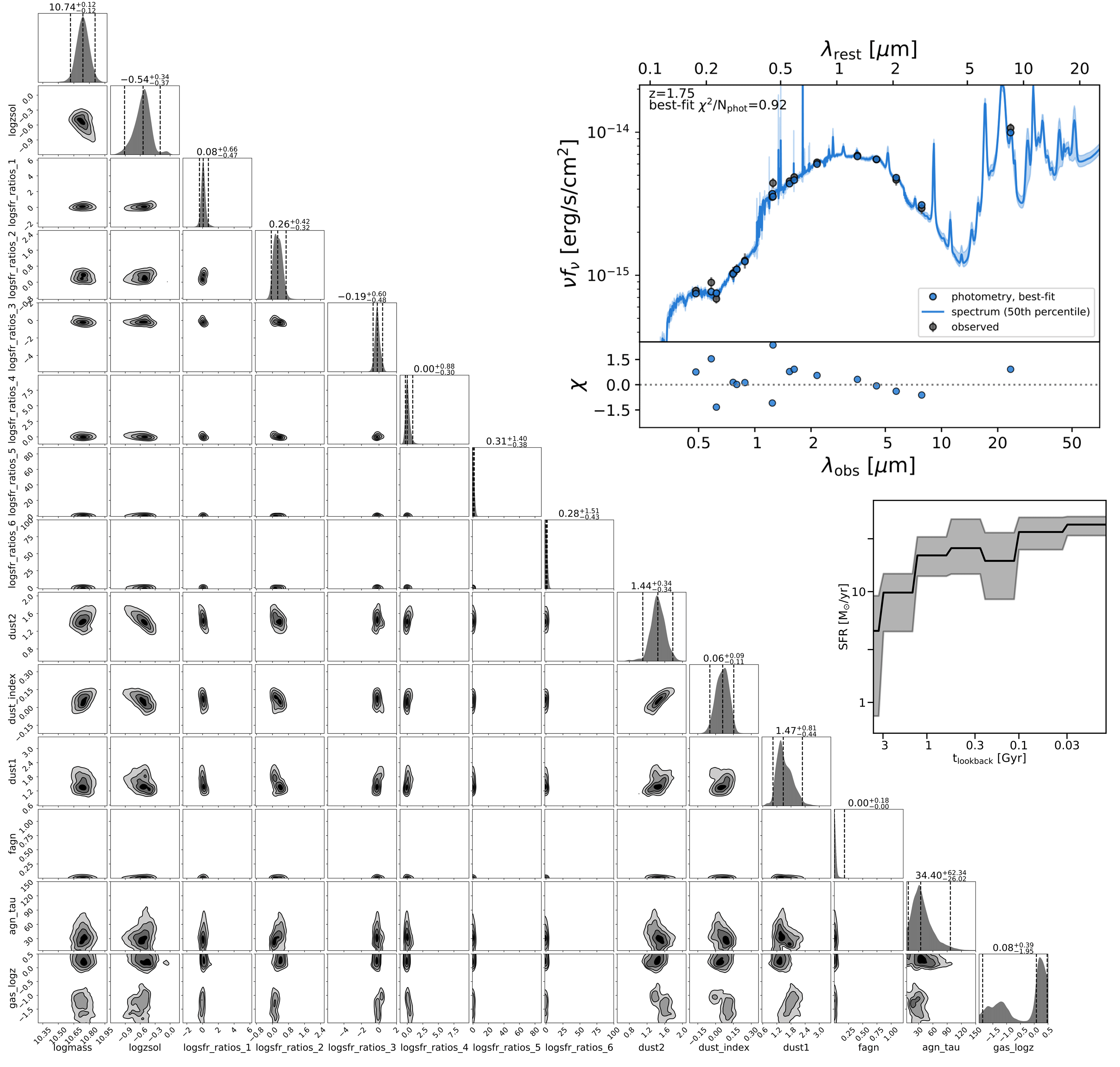
In Leja et al. (2018b), the authors modeled roughly 60k galaxy spectral energy distributions (SEDs) from the 3D-HST survey (Brammer et al., 2012) over a redshift range of . To conduct this analysis, they used the Bayesian SED fitting code Prospector (Johnson et al. in prep.), utilizing dynesty as their primary sampler, to sample from a 14-parameter model involving stellar mass, a non-parametric star formation history, stellar and gas metallicites, dust properties, and contributions from possible Active Galactic Nuclei. Compared to previous studies where emcee had been used to sample from the posterior (Leja et al., 2017, 2018c), the authors found that dynesty provided over an order of magnitude more efficient sampling and was able to characterize a wide variety of posteriors. The results for a typical galaxy are shown in Figure 11.
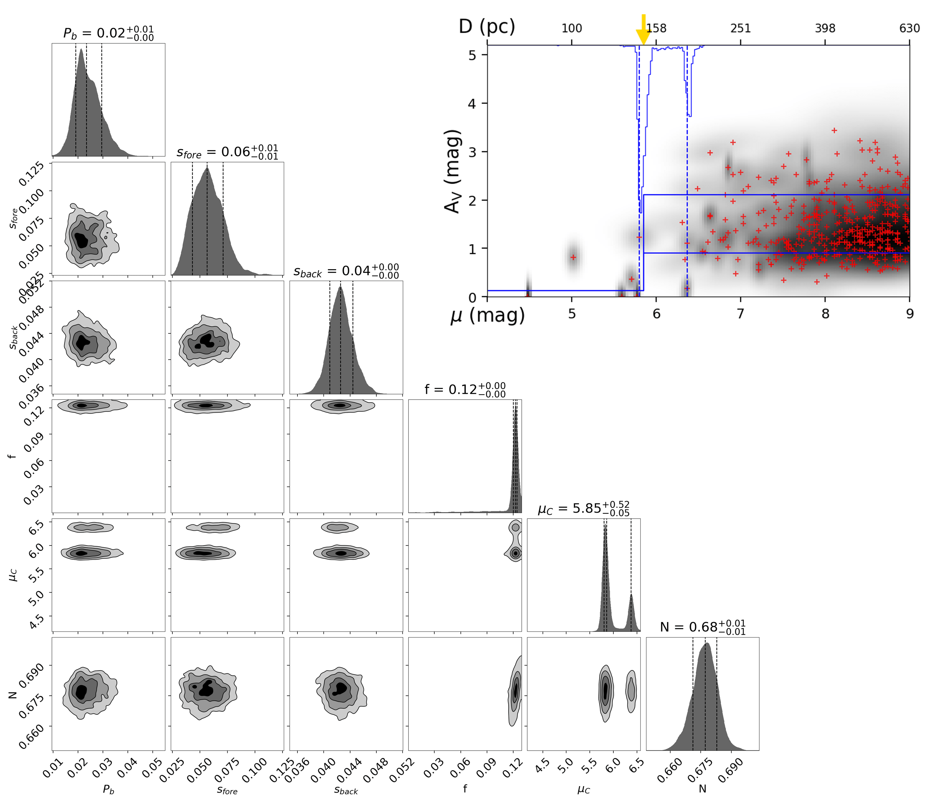
In Zucker et al. (2019), the authors used a combination of distance and reddening estimates to nearby stars from SED modeling (Speagle et al. in prep.) and Gaia parallax measurements (Gaia Collaboration et al., 2018) to derive distances to dozens of local molecular clouds. The distances to these clouds, however, are sensitive to the number and distribution of stars immediately in front of them as these stars help constrain the location of the “jump” in dust extinction associated with the cloud. In cases where there are only a small number of foreground stars, this constraint can be quite weak, leading to extended posteriors with multi-modal solutions. This, along with the overall performance illustrated in Figure 10, motivated the use of dynesty to sample from the 6-parameter cloud distance model used in the analysis. We highlight one such multi-modal case in Chameleon in Figure 12.
These examples, along with others listed earlier, are large-scale professional applications of dynesty that illustrate dynesty can work well in theory and in practice.
7 Conclusion
With Bayesian inference techniques now a large part of modern astronomical analyses, it has become increasingly important to develop and provide tools to the community that can help to “bridge the gap” between writing the underlying model and estimating the corresponding posterior . Tools such as emcee, MultiNest, and PolyChord, which provide Markov Chain Monte Carlo and Nested Sampling implementations, have been heavily used and highly cited.
In this paper we presented an overview of dynesty, a public, open-source, Python package that implements Dynamic Nested Sampling to enable flexible Bayesian inference over complex, multi-modal distributions. Building on previous work in the literature, we described the basics behind the Dyamic Nested Sampling approaches employed in the code, how we implement them, and how we use a variety of bounding and sampling methods to enable efficient inference. We then showcased dynesty’s performance on several toy problems as well as real astronomical application, highlighting its ability to estimate challenging posterior distributions both in theory and in practice.
While we have shown dynesty can perform similarly or better than existing MCMC approaches in one simple case, the real test for any package is based on users applying it to their analysis problems. We hope that dynesty will prove useful to the community and help facilitate exciting new science over the coming years.
Acknowledgements
JSS is grateful to Rebecca Bleich for her support and patience.
This project is the culmination of many individual efforts, not all of whom can be thanked here. First and foremost, JSS would like to thank Daniel Eisenstein, Charlie Conroy, and Doug Finkbeiner for their patience while he pursued this project, Catherine Zucker for her constant stream of feedback during development, and Johannes Buchner for incredibly insightful and inspiring conversations. JSS would also like to thank Johannes Buchner, Hannah Diamond-Lowe, Daniel Eisenstein, Daniel Foreman-Mackey, Will Handley, Ben Johnson, Joel Leja, Locke Patton, and Catherine Zucker for feedback on early drafts that substantially improved the quality of this work. JSS would further like to thank Johannes Buchner, Phil Cargile, Ben Cook, James Guillochon, and Ben Johnson for their direct and indirect contributions to the dynesty codebase, as well as Kyle Barbary and collaborators for their contributions to nestle (upon which dynesty was initially based). JSS is also grateful to many beta-testers who provided invaluable feedback during dynesty’s development and suffered through many bugfixes, including (but not limited to) Gregory Ashton, Ana Bonaca, Phil Cargile, Tansu Daylan, Hannah Diamond-Lowe, Philipp Eller, Jonathan Fraine, Maximilian Günther, Daniela Huppenkothen, Joel Leja, Sandro Tacchella, Ashley Villar, Catherine Zucker, and Joe Zuntz.
References
- Ashton et al. (2018) Ashton G., et al., 2018, arXiv e-prints, p. arXiv:1811.02042
- Betancourt (2017) Betancourt M., 2017, arXiv e-prints, p. arXiv:1701.02434
- Blei et al. (2016) Blei D. M., Kucukelbir A., McAuliffe J. D., 2016, arXiv e-prints,
- Blitzstein & Hwang (2014) Blitzstein J., Hwang J., 2014, Introduction to Probability. Chapman & Hall/CRC Texts in Statistical Science, CRC Press/Taylor & Francis Group, https://books.google.com/books?id=ZwSlMAEACAAJ
- Borne et al. (2009) Borne K., et al., 2009, in astro2010: The Astronomy and Astrophysics Decadal Survey. p. P6 (arXiv:0909.3892)
- Brammer et al. (2012) Brammer G. B., et al., 2012, The Astrophysical Journal Supplement Series, 200, 13
- Brewer et al. (2009) Brewer B. J., Pártay L. B., Csányi G., 2009, arXiv e-prints, p. arXiv:0912.2380
- Brooks et al. (2011) Brooks S., Gelman A., Jones G., Meng X.-L., 2011, Handbook of Markov Chain Monte Carlo. CRC press
- Buchner (2016) Buchner J., 2016, Statistics and Computing, 26, 383
- Buchner (2017) Buchner J., 2017, arXiv e-prints, p. arXiv:1707.04476
- Carpenter et al. (2017) Carpenter B., et al., 2017, Journal of Statistical Software, Articles, 76, 1
- Chopin & Ridgway (2015) Chopin N., Ridgway J., 2015, preprint, (arXiv:1506.08640)
- Chopin & Robert (2010) Chopin N., Robert C. P., 2010, Biometrika, 97, 741
- Diamond-Lowe et al. (2018) Diamond-Lowe H., Berta-Thompson Z., Charbonneau D., Kempton E. M. R., 2018, AJ, 156, 42
- Douc et al. (2005) Douc R., Cappé O., Moulines E., 2005, arXiv e-prints, p. cs/0507025
- Efron (1979) Efron B., 1979, Ann. Statist., 7, 1
- Espinoza et al. (2018) Espinoza N., Kossakowski D., Brahm R., 2018, arXiv e-prints, p. arXiv:1812.08549
- Feigelson (2017) Feigelson E. D., 2017, in Brescia M., Djorgovski S. G., Feigelson E. D., Longo G., Cavuoti S., eds, IAU Symposium Vol. 325, Astroinformatics. pp 3–9 (arXiv:1612.06238), doi:10.1017/S1743921317003453
- Feroz & Hobson (2008) Feroz F., Hobson M. P., 2008, MNRAS, 384, 449
- Feroz & Skilling (2013) Feroz F., Skilling J., 2013, in von Toussaint U., ed., American Institute of Physics Conference Series Vol. 1553, American Institute of Physics Conference Series. pp 106–113 (arXiv:1312.5638), doi:10.1063/1.4819989
- Feroz et al. (2009) Feroz F., Hobson M. P., Bridges M., 2009, MNRAS, 398, 1601
- Feroz et al. (2013) Feroz F., Hobson M. P., Cameron E., Pettitt A. N., 2013, preprint, (arXiv:1306.2144)
- Fisher (1922) Fisher R. A., 1922, Philosophical Transactions of the Royal Society of London Series A, 222, 309
- Foreman-Mackey (2016) Foreman-Mackey D., 2016, The Journal of Open Source Software, 24
- Foreman-Mackey et al. (2013) Foreman-Mackey D., Hogg D. W., Lang D., Goodman J., 2013, PASP, 125, 306
- Gaia Collaboration et al. (2018) Gaia Collaboration et al., 2018, A&A, 616, A1
- Gelman & Rubin (1992) Gelman A., Rubin D. B., 1992, Statistical Science, 7, 457
- Geman & Geman (1987) Geman S., Geman D., 1987, in Fischler M. A., Firschein O., eds, , Readings in Computer Vision. Morgan Kaufmann, San Francisco (CA), pp 564 – 584, doi:https://doi.org/10.1016/B978-0-08-051581-6.50057-X, %****␣dynesty.bbl␣Line␣175␣****http://www.sciencedirect.com/science/article/pii/B978008051581650057X
- Goodman & Weare (2010) Goodman J., Weare J., 2010, Communications in Applied Mathematics and Computer Science, 5, 65
- Guillochon et al. (2018) Guillochon J., Nicholl M., Villar V. A., Mockler B., Narayan G., Mandel K. S., Berger E., Williams P. K. G., 2018, The Astrophysical Journal Supplement Series, 236, 6
- Günther et al. (2019) Günther M. N., et al., 2019, arXiv e-prints, p. arXiv:1903.06107
- Handley et al. (2015) Handley W. J., Hobson M. P., Lasenby A. N., 2015, MNRAS, 450, L61
- Hastings (1970) Hastings W., 1970, Biometrika, 57, 97
- Heavens et al. (2017) Heavens A., Fantaye Y., Mootoovaloo A., Eggers H., Hosenie Z., Kroon S., Sellentin E., 2017, arXiv e-prints, p. arXiv:1704.03472
- Higson et al. (2017a) Higson E., Handley W., Hobson M., Lasenby A., 2017a, arXiv e-prints, p. arXiv:1703.09701
- Higson et al. (2017b) Higson E., Handley W., Hobson M., Lasenby A., 2017b, arXiv e-prints, p. arXiv:1704.03459
- Higson et al. (2019) Higson E., Handley W., Hobson M., Lasenby A., 2019, MNRAS, 483, 2044
- Hoffman & Gelman (2011) Hoffman M. D., Gelman A., 2011, arXiv e-prints, p. arXiv:1111.4246
- Hol et al. (2006) Hol J. D., Schon T. B., Gustafsson F., 2006, in 2006 IEEE Nonlinear Statistical Signal Processing Workshop. pp 79–82, doi:10.1109/NSSPW.2006.4378824
- Hunter (2007) Hunter J. D., 2007, Computing in Science Engineering, 9, 90
- Jasa & Xiang (2012) Jasa T., Xiang N., 2012, Acoustical Society of America Journal, 132, 3251
- Keeton (2011) Keeton C. R., 2011, MNRAS, 414, 1418
- Lartillot & Philippe (2006) Lartillot N., Philippe H., 2006, Systematic Biology, 55, 195
- Leja et al. (2017) Leja J., Johnson B. D., Conroy C., van Dokkum P. G., Byler N., 2017, ApJ, 837, 170
- Leja et al. (2018a) Leja J., Carnall A. C., Johnson B. D., Conroy C., Speagle J. S., 2018a, arXiv e-prints, p. arXiv:1811.03637
- Leja et al. (2018b) Leja J., et al., 2018b, arXiv e-prints, p. arXiv:1812.05608
- Leja et al. (2018c) Leja J., Johnson B. D., Conroy C., van Dokkum P., 2018c, ApJ, 854, 62
- Metropolis et al. (1953) Metropolis N., Rosenbluth A. W., Rosenbluth M. N., Teller A. H., Teller E., 1953, J. Chem. Phys., 21, 1087
- Mukherjee et al. (2006) Mukherjee P., Parkinson D., Liddle A. R., 2006, ApJ, 638, L51
- Nagaraja (2006) Nagaraja H. N., 2006, Order Statistics from Independent Exponential Random Variables and the Sum of the Top Order Statistics. Birkhäuser Boston, Boston, MA, pp 173–185, doi:10.1007/0-8176-4487-3_11, https://doi.org/10.1007/0-8176-4487-3_11
- Neal (2003) Neal R. M., 2003, Ann. Statist., 31, 705
- Neal (2012) Neal R. M., 2012, arXiv e-prints, p. arXiv:1206.1901
- Oliphant (2007) Oliphant T. E., 2007, Computing in Science Engineering, 9, 10
- Planck Collaboration et al. (2016) Planck Collaboration et al., 2016, A&A, 594, A20
- Plummer (2003) Plummer M., 2003, in Proceedings of the 3rd International Workshop on Distributed Statistical Computing.
- Salomone et al. (2018) Salomone R., South L. F., Drovandi C. C., Kroese D. P., 2018, arXiv e-prints, p. arXiv:1805.03924
- Sharma (2017) Sharma S., 2017, Annual Review of Astronomy and Astrophysics, 55, 213
- Shaw et al. (2007) Shaw J. R., Bridges M., Hobson M. P., 2007, MNRAS, 378, 1365
- Sivia & Skilling (2006) Sivia D., Skilling J., 2006, Data analysis: a Bayesian tutorial. Oxford science publications, Oxford University Press, https://books.google.com/books?id=6O8ZAQAAIAAJ
- Skilling (2004) Skilling J., 2004, in Fischer R., Preuss R., Toussaint U. V., eds, American Institute of Physics Conference Series Vol. 735, American Institute of Physics Conference Series. pp 395–405, doi:10.1063/1.1835238
- Skilling (2006) Skilling J., 2006, Bayesian Anal., 1, 833
- Skilling (2012) Skilling J., 2012, in Goyal P., Giffin A., Knuth K. H., Vrscay E., eds, American Institute of Physics Conference Series Vol. 1443, American Institute of Physics Conference Series. pp 145–156, doi:10.1063/1.3703630
- Trotta (2008) Trotta R., 2008, Contemporary Physics, 49, 71
- Vehtari et al. (2019) Vehtari A., Gelman A., Simpson D., Carpenter B., Bürkner P.-C., 2019, arXiv e-prints, p. arXiv:1903.08008
- York et al. (2000) York D. G., et al., 2000, AJ, 120, 1579
- Zucker et al. (2018) Zucker C., Schlafly E. F., Speagle J. S., Green G. M., Portillo S. K. N., Finkbeiner D. P., Goodman A. A., 2018, ApJ, 869, 83
- Zucker et al. (2019) Zucker C., Speagle J. S., Schlafly E. F., Green G. M., Finkbeiner D. P., Goodman A. A., Alves J., 2019, arXiv e-prints, p. arXiv:1902.01425
- van der Walt et al. (2011) van der Walt S., Colbert S. C., Varoquaux G., 2011, Computing in Science Engineering, 13, 22
Appendix A Detailed Nested Sampling Results
While we presented a broad overview of Nested Sampling in the main text, we glossed over much of the statistical background. We include more detailed results and discussion below.
The outline of these results are as follows. In §A.1 we outline the basic setup for Nested Sampling. In §A.2 we derive statistical properties in the single live point case. In §A.3 we discuss the process of utilizing multiple live points. In §A.4 we derive properties in the many live point case. In §A.5 we extend these results to encompass varying numbers of live points. Finally, in §A.6 we discuss various error properties of Nested Sampling as well as schemes to estimate them.
A.1 Setup
Following Skilling (2006), Feroz et al. (2013), and others, we start by (re-)defining Bayes Rule
| (51) |
where is the posterior, is the likelihood, is the prior, and
| (52) |
is the evidence.
To evaluate this integral, Nested Sampling seeks to transform it from one over position to one over prior volume where
| (53) |
defines the prior volume within a given iso-likelihood contour of level , assuming our priors are integrable, and
| (54) |
is the constrained prior. Note that since the integral over the entire prior is while the value as should approach if the maximum-likelihood value is a singular point.
Since , this allows us to redefine the evidence integral as
| (55) |
Provided the inverse of exists (i.e. there are no flat “slabs” of likelihood anywhere, only contours), we can rewrite this integral in terms of the prior volume associated with a particular iso-likelihood contour:
| (56) |
This is now a 1-D integral over that we can approximate using a discrete set of points using, e.g., a Riemann sum
| (57) |
where and is the (un-normalized) importance weight. These values can also be used to approximate the posterior:
| (58) |
A.2 Using a Single Live Point
Unfortunately, the exact value of at a given likelihood level is unknown. We can, however, construct an estimator with a known statistical distribution. Looking back at the definition of the prior volume , we see that it defines a cumulative distribution function (CDF) over . We can then define the associated probability density function (PDF) for as
| (59) |
Assuming we can sample from its PDF , we can use the Probability Integral Transform (PIT) to subsequently constrain the distribution of . In other words:
| (60) |
where notation implies the random variable is drawn from and is the standard Uniform distribution (i.e. flat from to ). This can be directly extended to cases where we are interested in sampling relative to a given threshold as
| (61) |
While this does not appear to make things any easier, it actually helps us out enormously. That’s because, at fixed , is actually a CDF over the constrained prior . That means we can bypass and altogether and just sample from directly to satisfy the PIT:
| (62) |
Various methods for sampling from the constrained prior subject to a suitable prior transform (see §2.2) are outlined in §4.
Before moving on, we want to quickly note that while the above scheme is sufficient for generating values of it is by no means necessary. As a counter-example, we can imagine a function that traces out a singular path through the distribution with support over . Let us furthermore assume that we construct such that we spend more “time” where the likelihood PDF is higher so that the PDF . Finally, let’s define the constrained function to simply be the portion of the path with . While this path by no means encompasses the prior, it is clear that
| (63) |
This result proves we can in theory satisfy the PIT for Nested Sampling using correlated samples provided they probe enough of the local portion of the prior to obtain sufficient coverage over the range of possible likelihoods (see also Salomone et al., 2018). It also provides support for why Nested Sampling works so well in practice even when samples are not fully independent.
For a given prior volume associated with a given likelihood level after iterations of this procedure, this implies the current prior volume will be
| (64) |
where
| (65) |
are independent and identically distributed (iid) random variables drawn from the standard Uniform distribution and we have taken . As we do not actually know the values of , we consider to be a noisy estimator of .
While sampling, we obviously need to assign a value for to determine, e.g., whether to stop. While we can easily simulate random values of , if we want these values to be consistent then a reasonable choice is the expectation value (arithmetic mean):
| (66) |
Alternately, we might also be interested in the expectation value of (geometric mean):
| (67) |
where we have used the fact that
| (68) |
where is the standard Exponential distribution and
| (69) |
A.3 Combining Live Points
Following Higson et al. (2017a), let’s consider the case where we have two independent live points following the basic sampling approach described above. These each form a set of samples with increasing likelihood
where the superscript notation indicates the index of the associated live point. We now want to “merge” these two sets of ordered samples together to get a single hypothetical ordered list:
where .
Independently, we know that the prior volume at a given iteration for each live point is just
What we want to know, however, is the distribution of of the merged list. Considering each sample independently implies and follow the same distribution (i.e. the first sampled prior volume for each run is similarly distributed). However, considering them together (based on the merged list) implies is strictly less than since . This tells us that cannot follow the same distribution from the associated independent runs that comprise it.
With this finding in hand, we now consider an approach for sampling from the prior volume using two live points. At each iteration , we remove the one with the lowest likelihood and replace it with a new point sampled from the constrained prior . After iterations, we will end up with a sorted list of likelihoods . If, however, we look at each live point individually (i.e. ignoring the other live point), we would find that each live point’s evolution would comprise a list of independent samples with ordered likelihoods that would each be identical to and , respectively! Therefore, we see that this procedure for sampling with two live points is identical to combining two sets of independent samples derived using one live point each.
A.4 Using Many Live Points
Now that we have established a procedure for running Nested Sampling with live points, we need to characterize how this affects our estimates of the prior volume. At any given iteration , we know that the current set of prior volumes associated with our live points are uniformly distributed within the prior volume from the previous iteration so that
| (70) |
where
| (71) |
We are now want to replace the live point with the lowest likelihood corresponding to the largest prior volume. This means we are now interested in the ordered list of prior volumes
| (72) |
where now indicates the position in the ordered list (from smallest to largest) rather than the live point index and
| (73) |
is the th standard uniform order statistic, where selects the th smallest point (so is the smallest and is the largest).
Using the Renyí Representation, it can be shown that we can represent the joint distribution of our standard uniform order statistics such that (Nagaraja, 2006):
| (74) |
where
| (75) |
The marginal distribution for is then (Blitzstein & Hwang, 2014):
| (76) |
where is the Beta distribution.
Using these results, we see that the prior volume based on live points at iteration evolves as
| (77) |
where are iid draws of the th standard uniform order statistic with marginal distribution . The arithmetic mean is
| (78) |
The geometric mean is
| (79) |
As discussed in §2.3, after we terminate sampling we can add the final set of live points to our set of samples. These will then just follow the final set of standard uniform order statistics relative to with an arithmetic mean
| (80) |
and geometric mean
| (81) |
where is the digamma function.
A.5 Using a Varying Number of Live Points
As discussed in §3, there’s no inherent reason why the number of number of live points must remain constant from iteration to iteration. Indeed, we can interpret adding the final set of live points to the list of samples from §A.4 as simply allowing the nested sampling run to continue while continually decreasing the number of live points. From this viewpoint, we have live points over iteration to , but only live points at iteration .
The change in the number of live points also changes the overall behavior of the Nested Sampling run before and after adding the final set of live points. We can highlight these by rewriting the results from §A.4 as:
| (82) |
This neatly decomposes the two “modes” in which Nested Sampling can traverse the prior. While “replacing” the worst live point (i.e. ), the prior volume shrinks exponentially by a constant factor at each iteration. However, when “removing” live points (i.e. ), we instead shrink uniformly by a variable factor at each iteration.
We can now generalize this behavior to the case where is allowed to vary at each iteration (Higson et al., 2017b). This now generates two distinct classes of behavior. When , we add live points to our existing set of live points, after which we replace the one with the worst likelihood . This then gives a distribution for the prior volume shrinkage of .
If , on the other hand, we instead have removed live points from the previous set of live points. The expected shrinkage is then based on the associated standard uniform order statistic from the initial set of values. Although in theory we should consider cases where the number of live points can decrease by an arbitrary amount, in practice when following iterative schemes such as the one outlined in Algorithm 3 we only need to consider the case where .
Taken together, these two types of behavior then give a mean estimate of:
| (83) | |||
where is the number of contiguous samples for which either exponential or uniform shrinkage dominates, is the total number of iterations that have occurred up to that point, and is the number of contiguous regions prior to iteration where one mode of shrinkage dominates. Note that for illustrative purposes here we have assumed the final samples are experiencing uniform shrinkage.
To summarize, varying the number of live points at each iteration simply involves dynamically switching between exponential and uniform shrinkage over the course of a Nested Sampling run. While this adds additional bookkeeping, it remains straightforward to estimate the prior volume at any particular iteration.
A.6 Nested Sampling Errors
We now turn our attention to characterizing various error properties of Nested Sampling, following the basic approach of Higson et al. (2017a, 2019). Similar to other sampling approaches, we expect some amount of “sampling noise” in our evidence and posterior estimates arising from the fact that we are approximating a continuous distribution (and smooth integral) with a discrete set of samples. We expect that as the number of live points at each iteration such that change in prior volume and the total number of samples , these sampling errors will become negligible.
Unlike other sampling approaches such as Markov Chain Monte Carlo (MCMC), however, Nested Sampling, contains an additional source of noise arising from our use of noisy estimators of the prior volume at a given iteration (Skilling, 2006). This “statistical noise” translates to a noisy estimator of the importance weight , which in turn gives noisy estimators for our previous evidence estimate
| (84) |
and our previous posterior estimate
| (85) |
Similar with the sampling noise, we also expect the statistical noise to become negligible as the number of live points at each iteration such that our estimate and the total number of samples .
We can highlight the decomposition of these two noise sources by considering trying to evaluate the expectation value of a target function with respect to the posterior (Chopin & Robert, 2010; Higson et al., 2017a):
| (86) |
where
| (87) |
is the expectation value of on the associated iso-likelihood contour with respect to the prior . Using the same Riemann sum approximation as §A.1, Nested Sampling would approximate this integral as:
| (88) | ||||
| (89) | ||||
| (90) |
We can see the two error types enter in cleanly through the final two approximations. In equation (89), we introduce sampling noise by replacing , which is averaged over the entire iso-likelihood contour, with the estimate evaluated at a single point. Then, in equation (90), we replace the true importance weight at a given prior volume with its noisy estimate based on our noisy estimators for the prior volume .
A.6.1 Statistical Uncertainties
In §A.2, §A.4, and §A.5, we derived the analytic distribution for our prior volume estimator at iteration under a variety of assumptions. While the distribution for and is not analytic, it is straightforward to draw from them. First, we simulate values of the prior volumes
| (91) |
by drawing a combination of -distributed random variables (when ) and standard uniform order statistics (when ) and iteratively computing each using the procedures outlined earlier. Then, we simply compute the corresponding evidence and posterior estimates.
While we can simulate the prior volumes and trace their impact on and explicitly, it is also helpful to derive a rough estimate of their impact. Since the posterior can be arbitrarily complex, we will focus on the evidence for which this analysis is more tractable.
There have previously been two main approaches for deriving the uncertainty, which focus either on trying to derive (Keeton, 2011) or (Skilling, 2006). Here we will focus on the latter, which gives a cleaner (if less precise) result.
We first start with the Static Nested Sampling case using a constant number of live points . To estimate the evidence , we must integrate over the unnormalized posterior . This occurs after a certain number of iterations have passed given a fixed stopping criterion.
There are two factors that contribute to the overall . The first is the rate of integration: at any given iteration , the prior volume decreases by . As a result, it must be the case that .
The second is the total amount of prior volume that needs to be integrated over. This roughly scales as the Kullback-Leibler (KL) divergence (i.e. “information gain”) between the prior and posterior
| (92) | ||||
| (93) |
Since is a discrete number that is typically large, it is reasonable to assume that it follows a Poisson distribution such that
| (94) |
This leads to a rough uncertainty in of
| (95) |
We now extend this result to encompass a variable number of live points at each iteration. We first rewrite our estimate of the variance as
| (96) |
where the final approximation assumes the distribution of evidence updates is independent at each iteration and . If we further assume that the distribution of the actual evidence estimates themselves are roughly independent at each iteration and that the number of live points changes sufficiently slowly such that , we find
| (97) |
Substituting this in to our original expression and taking then gives a modified error estimate
| (98) |
While the modified estimator in equation (98) is less reliable that our original estimate, it is somewhat reassuring that in the special case it reduces to the original estimator derived in equation (95).
A.6.2 Sampling Uncertainties
Unlike the statistical uncertainties on the prior volume estimator , we do not have analytic expression or ways to explicitly simulate from the distribution characterized by our sampling uncertainties. In fact, it is doubtful we will ever have access to these except in special cases, since they rely on having access to the distribution of all possible paths (or varying lengths) live points can take through the distribution over the course of a Nested Sampling run.
This however, does not mean we cannot attempt to construct an estimate of this distribution. To do this, we follow Higson et al. (2017a) and turn to bootstrapping, which serves as a generic and robust tool for attempting to simulate the impact of sampling uncertainties with limited support (Efron, 1979). Since in most cases we have many thousands of samples from our distribution and sample with live points, Nested Sampling is almost always in a regime where bootstrapping should be viable.
Naively, we might expect to simply be able simulate values of, e.g., by just bootstrapping the underlying set of live points. However, this leads to three immediate complications:
-
1.
This approach creates multiple samples at the same position. It is unclear how these points need to be ordered to assign them associated prior volumes.
-
2.
This approach conserves the total number of samples , which clearly must be allowed to change if we really want to simulate from all possible live point paths (with varying path-lengths).
-
3.
This approach can leave out samples initially drawn from the prior. These points are crucial for establishing the normalization needed to estimate the evidence, and so removing them drastically distorts our evidence estimates.
We address each of these in turn.
First, the ambiguous ordering, while at first glance a serious issue, is actually a non-concern since the impact on any derived quantity is actually completely insensitive to the ordering. For the evidence, since the likelihood is identical among the points, their contribution to will remain unchanged. Likewise, because they occupy the same position , their contribution to the posterior estimate is also unchanged. This implies that any ordering scheme (e.g., random) will suffice.
To resolve the second issue, we now turn to the problem of simulating all possible live point paths along with their possibly varying path-lengths. Bootstrapping over all the samples by construction destroys this information by ignoring the paths of each individual live point. Analogous to the discussion in §A.3, we can characterize these individual paths as being the collection of lists of positions traversed by each live point. Sampling from the space of all possible live point paths thus is equivalent to bootstrapping from these individual “strands” and then merging the resampled strands into a new Nested Sampling run.
Unfortunately, this procedure still can run afoul of the third issue when the number of live points is not constant. Going back to the discussion in §A.3 and the Iterative Dynamic Nested Sampling scheme outlined in Algorithm 3, we see that increasing the number of live points at some iteration means that those additional live points were sampled interior to the prior at some associated likelihood threshold . Since these live points provide no information about the overall normalization (only the normalization relative to ), they are totally uninformative on their own when it comes to estimating the evidence .
To account for this, we need to perform a stratified bootstrap over the set of “interior” strands (i.e. strands with starting positions interior to the prior) and “anchor” strands (i.e. strands sampled directly from the prior that “anchor” the interior strands). Once the set of interior strands and strands have been resampled, we can then merge the new collection into a new Nested Sampling run. Following this scheme is then sufficient for simulating the evidence and posterior estimates, where we have used notation to indicate a we used bootstrapping rather than prior volume simulation.
Note that one interesting corollary of our bootstrap estimates is that we expect the total number of samples to change. For a sufficient number of live points, this distribution is likely to be roughly Poisson. Assuming that the associated and from our bootstrapped Nested Sampling run are similar to the original, this immediately leads us to an estimate of identical to that in equation (98). Although it has the exact same form, note that this error term is completely independent from the previous case.
A.6.3 Combined Uncertainties
The full uncertainties associated with a given Nested Sampling run involve both the statistical uncertainties described in §A.6.1 and the sampling uncertainties described in §A.6.2. Simulating from this combined error distribution is straightforward and can be done by the following procedure:
-
1.
Resample the set of underlying anchor and interior strands using stratified bootstrap resampling.
-
2.
Merge the resampled strands into a single run.
-
3.
Simulate the values of the prior volumes.
We can then calculate the evidence and posterior estimates accordingly. The combined uncertainty on the evidence that we estimate from both sources is then roughly
| (99) |
based on the identical error estimates derived in §A.6.1 and §A.6.2.