Towards the routine use of subdominant harmonics in gravitational-wave inference:
re-analysis of GW190412 with generation X waveform models

Abstract

We re-analyse the gravitational-wave event GW190412 with state-of-the-art phenomenological waveform models. This event, which has been associated with a black hole merger, is interesting due to the significant contribution from subdominant harmonics. We use both frequency-domain and time-domain waveform models. The PhenomX waveform models constitute the fourth generation of frequency-domain phenomenological waveforms for black hole binary coalescence; they have more recently been complemented by the time-domain PhenomT models, which open up new strategies to model precession and eccentricity, and to perform tests of general relativity with the phenomenological waveforms approach. Both PhenomX and PhenomT have been constructed with similar techniques and accuracy goals, and due to their computational efficiency this “generation X” model family allows the routine use of subdominant spherical harmonics in Bayesian inference. We show the good agreement between these and other state-of-the-art waveform models for GW190412, and discuss the improvements over the previous generation of phenomenological waveform models. We also discuss practical aspects of Bayesian inference such as run convergence, variations of sampling parameters, and computational cost.

I Introduction

The analysis of gravitational wave (GW) data from compact binary coalescences (CBCs) has long focused on the dominant quadrupole spherical harmonics, and the use of sub-dominant spherical harmonics has only recently started to play a prominent role for observational results Abbott et al. (2020a, b); Abbott and et. al. (2020a, b) with the ground-based detectors Advanced LIGO Aasi et al. (2015) and Advanced Virgo Acernese et al. (2015). The use of waveform models including sub-dominant harmonics can often break degeneracies between source parameters and improve the overall parameter estimation results even if the content of sub-dominant harmonics is weak for the most likely set of parameters, since the additional harmonics help to exclude parameter-space regions which are not consistent with the data under the more complete models.

Here we argue that models including subdominant harmonics should now be used routinely in GW parameter estimation, and how this is facilitated by the computational efficiency and accuracy of the “generation X” of phenomenological waveform models: the frequency-domain IMRPhenomX models Pratten et al. (2020a); García-Quirós et al. (2020, 2020); Pratten et al. (2020b), and the complementary time-domain IMRPhenomT models Estellés et al. (2020); Estellés and et. al. (2020). In particular we demonstrate the capability of the generation X waveform family to deliver a suite of Bayesian inference results both quickly, and with relatively low total computational cost. One interesting application is on measuring the source distance, where breaking the degeneracy with the binary’s inclination through inclusion of subdominant harmonics significantly improves accuracy Kalaghatgi et al. (2020); Abbott et al. (2020a). A quick turnaround on such precise distance measurements is particularly important in the context of electromagnetic counterparts, which have recently become more interesting also in the context of binary black hole (BBH) mergers, as discussed in connection with the discovery of GW190521 Abbott and et. al. (2020a, b). Moreover, being able to efficiently compare posteriors for multiple models from the same family including different amount of physics (aligned spins only vs. precession, dominant modes only vs. inclusion of subdominant modes) allows detailed studies of waveform modelling systematics, increasing the confidence in the final parameter estimates for an event.

To provide a guide to the routine use of subdominant harmonics in practical parameter estimation and to demonstrate the capabilities of the “generation X” phenomenological waveform models on a specific example, in this paper we present improved parameter estimation results for the event GW190412 first published in Abbott et al. (2020a). GW190412 is special among the CBC observations reported by LIGO and Virgo to date Abbott et al. (2019a, 2020c, 2020a, 2020b); Abbott and et. al. (2020a) as the first BBH signal with clear evidence for significantly unequal component masses. Since the effect of sub-dominant spherical harmonic modes is stronger in unequal-mass systems, this event also provided the first observational evidence for their presence. On the other hand, as for previous BBH detections, only limited amounts of information about the spins of the black holes could be extracted in Abbott et al. (2020a). The event is of astrophysical interest as the unusual mass ratio hints at a more diverse population of merging BBHs in the Universe than the ‘vanilla’ events previously observed Abbott et al. (2019a, b) and starts to provide discriminating evidence between possible formation channels for these systems Abbott et al. (2020a); Mandel and Fragos (2020); Di Carlo et al. (2020); Olejak et al. (2020); Hamers and Safarzadeh (2020); Rodriguez et al. (2020); Gerosa et al. (2020); De Luca et al. (2020); Safarzadeh and Hotokezaka (2020); Kimball et al. (2020).

In general, the measurement of CBC source properties through matched filtering and Bayesian inference relies crucially on the quality of the waveform models used as the templates. Waveform models are typically synthesized from perturbative results (notably the post-Newtonian Blanchet (2006) and effective-one-body Damour (2001); Damour et al. (2013); Cotesta et al. (2018) frameworks and results for the ringdown frequencies of Kerr black holesBerti et al. (2006)), and catalogues of numerical relativity (NR) simulations, such as the large catalogue of waveforms from the SXS collaboration SXS Collaboration (2019); Boyle et al. (2019). Several such models of varying complexity have been used in Abbott et al. (2020a) to measure the source properties of GW190412. None of those models includes orbital eccentricity, but two of them include both precession and subdominant harmonics: the frequency-domain model IMRPhenomPv3HM Khan et al. (2020) and the time-domain model SEOBNRv4PHM Ossokine et al. (2020). Both are members of families of models which also include simpler models without precession or subdominant harmonics, which have been used for model comparison to determine the evidence for the presence of these effects in the data. Systematic errors in such waveform models, in particular regarding precession and sub-dominant harmonics, are not yet well understood, and the high computational cost for both the IMRPhenomPv3HM and SEOBNRv4PHM models is one reason why investigations of potential systematics are challenging. None of the models used to analyze GW190412 in Abbott et al. (2020a) is calibrated to precessing NR waveforms, and only in SEOBNRv4PHM have the subdominant harmonics been calibrated to NR, with IMRPhenomPv3HM using approximate scalings to include their effects.

Our re-analysis of GW190412 focuses on the IMRPhenomX family of inspiral-merger-ringdown waveform models Pratten et al. (2020a); García-Quirós et al. (2020, 2020); Pratten et al. (2020b) which constitute a thorough upgrade of previous versions of the family of frequency-domain phenomenological waveform models Husa et al. (2016); Khan et al. (2016); Hannam et al. (2014); Bohé et al. (2016); London et al. (2018); Khan et al. (2019, 2020) that is currently routinely used in CBC data analysis, including the IMRPhenomPv3HM model mentioned above. In addition we study this event with the new IMRPhenomT family of phenomenological time-domain waveforms (with the versions currently implemented in the LALSuite LIGO Scientific Collaboration (2020) package not yet including precession). An alternative re-analysis focusing on the NRSur7dq4 Varma et al. (2019a) model has been presented in Islam et al. (2020). NRSur7dq4 is based on reduced-order-modelling (ROM) Pürrer (2014) and has been calibrated to numerical relativity waveforms. It does however not span a sufficiently wide frequency range to cover the entire LIGO and Virgo bands for the mass range of GW190412, and Islam et al. (2020) studies variations of the lower cutoff frequency.

None of the IMRPhenomX models have yet been calibrated to precessing NR waveforms, but IMRPhenomXHM, IMRPhenomXPHM and IMRPhenomTHM are calibrated to sub-dominant harmonics from NR waveforms. The modularity and flexibility of the model family allows to compare different approximations for the effects of spin precession and different choices for the final spin of the remnant black hole. Furthermore the drastically reduced computational cost of the new waveforms allows us to test in detail the impact of varying some of the settings of the Bayesian sampling algorithms we use Ashton et al. (2019); Smith et al. (2019); Romero-Shaw et al. (2020). We find that by replacing IMRPhenomPv3HM with our upgraded precessing higher-modes model IMRPhenomXPHM, the disagreement between the frequency and time-domain models observed in Abbott et al. (2020a) can be reduced significantly, and the uncertainty intervals for key parameters can be tightened. The agreement between frequency and time-domain models is further improved when assuming that the source does not show significant spin-precession, which we confirm to be consistent with the observational data. A summary of our parameter estimation results and a comparison with the results from Abbott et al. (2020a) can be found in Table 1 and is discussed below.

The paper is organized as follows. In Sec. II we collect preliminaries: remarks on notation, a summary of the results found in Abbott et al. (2020a) on the event GW190412 and brief descriptions of the different waveform models and Bayesian inference methods used there and in the present paper. We then present our main parameter estimation results on GW190412 in Sec. III, further investigations on systematic and sampling errors in Sec. IV, and a summary and our conclusions in Sec. V. Further comparisons are presented in appendices: while all our main results are obtained with the parallel Bilby code Ashton et al. (2019); Smith et al. (2019); Romero-Shaw et al. (2020), in appendix A we also compare these results with comparison runs of the LALInference code Veitch et al. (2015). And in appendix B we compare our main Bilby runs, which have been obtained with marginalisation over distance in order to improve convergence, with runs that do not use this approximation. Different IMRPhenomX implementations of precession and approximations for the spin of the merger remnant are studied in appendix C. Finally, we compare results in more detail against the IMRPhenomPv3HM model in appendix D and study the impact of alternative spin priors in appendix E.

Posterior samples from our preferred run for each waveform model are released in Colleoni et al. (2020).

II Preliminaries

II.1 Notation and conventions

We will report all masses in units of the solar mass $M_{\odot}$. Masses are reported both in the detector frame, where they appear redshifted, and in the source frame, assuming a standard cosmology Planck Collaboration et al. (2016) (see Appendix B of Abbott et al. (2019a)). We will report source-frame masses with a superscript $\mathrm{s}$, as in $m_{1}^{\mathrm{s}}$ to denote the mass of the larger black hole in the source frame. We will drop the superscript to denote masses in the detector frame, and to represent general relations between different mass parameters. Individual component masses are denoted by $m_{i}$, the total mass is $M=m_{1}+m_{2}$, and the chirp mass by $\mathcal{M}=(m_{1}\,m_{2})^{3/5}M^{-1/5}$. The mass ratio is defined as $q=m_{2}/m_{1}\leq 1$.

We also define two effective spin parameters which are commonly used in waveform modelling and parameter estimation. First, the parameter $\chi_{\rm{eff}}$ Damour (2001); Ajith et al. (2011); Santamaria et al. (2010) is defined as

$$\chi_{\mathrm{eff}}=\frac{m_{1}\chi_{1}+m_{2}\chi_{2}}{m_{1}+m_{2}},$$ (1)

where the $\chi_{i}$ are the projections of the spin vectors of the individual black holes onto the orbital angular momentum. Second, the effective spin precession parameter $\chi_{p}$ Schmidt et al. (2015) has been designed to capture the dominant effect of precession. It corresponds to an approximate average over many precession cycles of the spin in the precessing orbital plane, and is defined in terms of the average spin magnitude $S_{p}$, Hannam et al. (2014); Schmidt et al. (2015)

$$S_{p} =\frac{1}{2}\left(A_{1}S_{1,\perp}+A_{2}S_{2,\perp}+|A_{1}S_{1,\perp}-A_{2}S_{2,\perp}|\right),$$ (2)

$$={\rm{max}}\left(A_{1}S_{1,\perp},A_{2}S_{2,\perp}\right),$$ (3)

where $A_{1}=2+3/(2q)$, and $\chi_{p}$ is then defined as

$$\chi_{p} =\frac{S_{p}}{A_{1}m^{2}_{1}}.$$ (4)

Both $\chi_{\mathrm{eff}}$ and $\chi_{p}$ are dimensionless and thus independent of the frame (source or detector).

Throughout this work we will employ waveforms with several multipoles beyond the quadrupolar contribution. Unless otherwise stated, we will consider pairs of both positive and negative modes when referring to a particular multipole. For example, to refer to a set of multipoles $(l,m)=(2,\pm 2),(2,\pm 1)$ we will use the simplified notation $(l,|m|)=(2,2),(2,1)$ or simply $(2,2),(2,1)$.

II.2 Summary of the event GW190412

Table 1: Inferred parameter values for GW190412 and their 90% credible intervals, obtained using precessing models including higher multipoles. Columns 2–4 correspond to the results from the LVC analyses Abbott et al. (2020a), the fifth column gives the new results from our preferred inference run, which is run 26 from Table 3 with the precessing higher-modes model IMRPhenomXPHM, and the last column combines the LVC SEOBNRv4PHM results with IMRPhenomXPHM in the same way that they were combined with IMRPhenomPv3HM in Abbott et al. (2020a).

parameter	SEOBNRv4PHM	IMRPhenomPv3HM	LVC Combined	IMRPhenomXPHM	Combined
$m_{1}^{\mathrm{s}}/M_{\odot}$	$31.7_{-3.5}^{+3.6}$	$28.1_{-4.3}^{+4.8}$	$29.7_{-5.3}^{+5.0}$	$30.0^{+5.2}_{-4.3}$	$30.9^{+4.3}_{-4.4}$
$m_{2}^{\mathrm{s}}/M_{\odot}$	$8.0_{-0.7}^{+0.9}$	$8.8_{-1.1}^{+1.5}$	$8.4_{-1.0}^{+1.8}$	$8.4^{+1.3}_{-1.1}$	$8.2^{+1.2}_{-0.9}$
$M^{\mathrm{s}}/M_{\odot}$	$39.7_{-2.7}^{+3.0}$	$36.9_{-2.9}^{+3.7}$	$38.1_{-3.7}^{+4.0}$	$38.4^{+4.2}_{-3.2}$	$39.1^{+3.6}_{-3.3}$
$\mathcal{M}^{\mathrm{s}}/M_{\odot}$	$13.3_{-0.3}^{+0.3}$	$13.2_{-0.3}^{+0.5}$	$13.3_{-0.3}^{+0.4}$	$13.3^{+0.5}_{-0.4}$	$13.3^{+0.4}_{-0.3}$
$q$	$0.25_{-0.04}^{+0.06}$	$0.31_{-0.07}^{+0.12}$	$0.28_{-0.06}^{+0.13}$	$0.28^{+0.09}_{-0.07}$	$0.27^{+0.09}_{-0.06}$
$M_{\mathrm{f}}/M_{\odot}$	$38.6_{-2.8}^{+3.1}$	$35.7_{-3.0}^{+3.8}$	$37.0_{-3.9}^{+4.1}$	$37.2_{-3.3}^{+4.3}$	$38.0^{+3.5}_{-3.3}$
$\chi_{\mathrm{f}}$	$0.68_{-0.04}^{+0.04}$	$0.67_{-0.07}^{+0.07}$	$0.67_{-0.07}^{+0.05}$	$0.67_{-0.05}^{+0.05}$	$0.67^{+0.05}_{-0.04}$
$m_{1}/M_{\odot}$	$36.5_{-4.2}^{+4.2}$	$32.3_{-5.2}^{+5.7}$	$34.2_{-6.5}^{+5.7}$	$34.4^{+6.2}_{-5.1}$	$35.5^{+5.2}_{-5.1}$
$m_{2}/M_{\odot}$	$9.2_{-0.7}^{+0.9}$	$10.1_{-1.2}^{+1.6}$	$9.7_{-1.1}^{+1.8}$	$9.6^{+1.4}_{-1.2}$	$9.4^{+1.3}_{-0.9}$
$M/M_{\odot}$	$45.7_{-3.3}^{+3.5}$	$42.5_{-3.7}^{+4.4}$	$43.9_{-4.7}^{+4.6}$	$44.1^{+5.0}_{-3.7}$	$44.9^{+4.3}_{-3.8}$
$\mathcal{M}/M_{\odot}$	$15.3_{-0.2}^{+0.1}$	$15.2_{-0.2}^{+0.3}$	$15.3_{-0.2}^{+0.2}$	$15.3^{+0.4}_{-0.2}$	$15.3^{+0.3}_{-0.2}$
$\chi_{\rm eff}$	$0.28_{-0.08}^{+0.06}$	$0.22_{-0.11}^{+0.08}$	$0.25_{-0.11}^{+0.08}$	$0.25^{+0.1}_{-0.1}$	$0.26^{+0.08}_{-0.09}$
$\chi_{\mathrm{p}}$	$0.31_{-0.15}^{+0.14}$	$0.31_{-0.17}^{+0.24}$	$0.30_{-0.15}^{+0.19}$	$0.23^{+0.20}_{-0.13}$	$0.27^{+0.17}_{-0.15}$
$\chi_{1}$	$0.46_{-0.15}^{+0.12}$	$0.41_{-0.24}^{+0.22}$	$0.43_{-0.26}^{+0.16}$	$0.39^{+0.16}_{-0.17}$	$0.43^{+0.14}_{-0.17}$
$D_{\mathrm{L}}/\textrm{Mpc}$	$740_{-130}^{+120}$	$740_{-190}^{+150}$	$730_{-170}^{+140}$	$734^{+161}_{-187}$	$737^{+141}_{-159}$
$z$	$0.15_{-0.02}^{+0.02}$	$0.15_{-0.04}^{+0.03}$	$0.15_{-0.03}^{+0.03}$	$0.15_{-0.04}^{+0.03}$	$0.15_{-0.03}^{+0.03}$
$\hat{\theta}_{JN}$	$0.71_{-0.21}^{+0.23}$	$0.71_{-0.27}^{+0.39}$	$0.73_{-0.24}^{+0.34}$	$0.75^{+0.36}_{-0.28}$	$0.73^{+0.31}_{-0.24}$
$\rho_{\mathrm{H}}$	$9.5_{-0.2}^{+0.1}$	$9.5_{-0.3}^{+0.2}$	$9.5_{-0.3}^{+0.1}$	$9.4^{+0.2}_{-0.3}$	$9.4^{+0.2}_{-0.3}$
$\rho_{\mathrm{L}}$	$16.2_{-0.2}^{+0.1}$	$16.1_{-0.3}^{+0.2}$	$16.2_{-0.3}^{+0.1}$	$16.1^{+0.2}_{-0.3}$	$16.2^{+0.2}_{-0.3}$
$\rho_{\mathrm{V}}$	$3.7_{-0.5}^{+0.2}$	$3.6_{-1.0}^{+0.3}$	$3.6_{-1.0}^{+0.3}$	$3.6^{+0.3}_{-0.8}$	$3.7^{+0.3}_{-0.7}$
$\rho_{\mathrm{HLV}}$	$19.1_{-0.2}^{+0.2}$	$19.0_{-0.3}^{+0.2}$	$19.1_{-0.3}^{+0.1}$	$18.9_{-0.3}^{+0.2}$	$19.0_{-0.4}^{+0.2}$

GW190412 is the first BBH detection from the O3 observing run published Abbott et al. (2020a) by the LIGO-Virgo Collaboration (LVC). It was observed by all three detectors, with a network signal-to-noise ratio (SNR) of $19.1_{-0.3}^{+0.1}$ from the final coherent Bayesian analysis reported in Abbott et al. (2020a). In briefly summarizing the event properties, we concentrate here on the results from Bayesian inference using the Bilby Ashton et al. (2019); Smith et al. (2019); Romero-Shaw et al. (2020), LALInference Veitch et al. (2015) and RIFT Lange et al. (2018); Wysocki et al. (2019) packages and the SEOBNRv4PHM Ossokine et al. (2020) and IMRPhenomPv3HM Khan et al. (2020) waveform models. These LVC estimates of the properties of GW190412’s source are listed in Table 1 together with our own results.

In summary, GW190412 came from a BBH with individually unremarkable source-frame masses $m_{1}^{\mathrm{s}}\approx 30M_{\odot}$ and $m_{2}^{\mathrm{s}}\approx 8M_{\odot}$, but the mass ratio $q=m_{2}/m_{1}\approx 0.3$ ($<0.5$ at 99% probability) is much lower than inferred for any previous detection. The system’s effective spin parameter appears to be low, but significantly different from zero: $\chi_{\mathrm{eff}}=0.25_{-0.11}^{+0.08}$ when combining results from both waveforms. The effective precession parameter has also been constrained, but more weakly, to $\chi_{\mathrm{p}}=0.31_{-0.16}^{+0.19}$. While there is some information gain compared to the prior on this quantity, and the posterior is peaked away from zero, it prefers lower values than the prior. The results from SEOBNRv4PHM and IMRPhenomPv3HM agree within 90% uncertainties for all quantities reported in Abbott et al. (2020a), but do show some qualitative differences – for example,

the IMRPhenomPv3HM posteriors tend to less unequal $q$ together with lower $\chi_{\mathrm{eff}}$.

Additional inference runs were also reported in Abbott et al. (2020a) for several waveform models with reduced physics content (see their Table I and references therein), with the goal of estimating the evidence for the presence of precession and HMs in the observed signal. Clear and robust evidence was found for the presence of HMs, with $\log_{10}$ Bayes factors between 3.0 and 4.1 in favour of models including HMs over those only including $\ell=2$ modes, depending on the waveform model family, sampling method and whether precession was also included at the same time. On the other hand, there was no clear evidence for or against precession, with the obtained Bayes factors for that hypothesis test remaining within systematic uncertainties for each waveform model family. We summarise Bayes factors listed in the LVC publication, together with those obtained from our own analysis, in Table 4.

The main astrophysical conclusions that Abbott et al. (2020a) drew from GW190412 include that the event’s properties, especially its mass ratio, are somewhat unexpected for draws from a BBH population as inferred from the previous two observing runs Abbott et al. (2019a, b), but not in clear tension with it. Furthermore, the formation of the source system challenges some astrophysical models that mostly predict mergers with near-equal masses, but GW190412 is still compatible with most versions of both isolated binary evolution and dynamical assembly Postnov and Yungelson (2014); Benacquista and Downing (2013). Implications for specific formation scenarios have since been the topic of many studies Mandel and Fragos (2020); Di Carlo et al. (2020); Olejak et al. (2020); Hamers and Safarzadeh (2020); Rodriguez et al. (2020); Gerosa et al. (2020); De Luca et al. (2020); Safarzadeh and Hotokezaka (2020), and more accurate and robust inference of the system’s mass and spin parameters can be crucial in further constraining these channels.

Additional PE analyses of GW190412 have also been reported by Zevin et al. (2020), focusing on the impact of alternative spin priors, and recently by Islam et al. (2020), focusing on the NRSur7dq4 model and the effect of varying the lower cutoff frequency.

II.3 Waveform models used

Table 2: Waveform models used in this paper. We indicate which models include precession and which multipoles are included for each model. For precessing models, the multipoles correspond to those in the co-precessing frame.

family	full name	precession	multipoles $(\ell,\,|m|)$	ref.
EOBNR	SEOBNRv4HM_ROM	$\times$	(2, 2)	Bohé et al. (2017)
	SEOBNRv4_ROM	$\times$	(2, 2), (2,1), (3, 3), (4, 4), (5,5)	Cotesta et al. (2018, 2020)
	SEOBNRv4P	✓	(2, 2), (2, 1)	Ossokine et al. (2020); Babak et al. (2017); Pan et al. (2014)
	SEOBNRv4PHM	✓	(2, 2), (2, 1), (3, 3), (4, 4), (5,5)	Ossokine et al. (2020); Babak et al. (2017); Pan et al. (2014)
Phenom - Gen. 3	IMRPhenomD	$\times$	(2, 2)	Husa et al. (2016); Khan et al. (2016)
	IMRPhenomHM	$\times$	(2, 2), (2, 1), (3, 3), (3, 2), (4,4), (4, 3)	London et al. (2018)
	IMRPhenomPv2	✓	(2, 2)	Hannam et al. (2014); Bohé et al. (2016)
	IMRPhenomPv3	✓	(2, 2)	Khan et al. (2019)
	IMRPhenomPv3HM	✓	(2, 2), (2, 1), (3, 3), (3, 2),(4, 4), (4, 3)	Khan et al. (2020)
NR surrogate	NRHybSur3dq8	$\times$	$\ell\leq 4$, (5, 5) but not (4, 0), (4, 1)	Varma et al. (2019b)
PhenomX	IMRPhenomXAS	$\times$	(2, 2)	Pratten et al. (2020a)
	IMRPhenomXHM	$\times$	(2, 2), (2, 1), (3, 3), (3, 2), (4,4)	García-Quirós et al. (2020, 2020)
	IMRPhenomXP	✓	(2, 2)	Pratten et al. (2020b)
	IMRPhenomXPHM	✓	(2, 2), (2, 1), (3, 3), (3, 2),(4, 4)	Pratten et al. (2020b)
PhenomT	IMRPhenomT	$\times$	(2, 2)	Estellés et al. (2020)
	IMRPhenomTHM	$\times$	(2, 2), (2, 1), (3, 3), (4,4), (5,5)	Estellés and et. al. (2020)

CBC parameter estimation currently mostly uses waveform models from three different families:

• Models constructed within the effective-one-body (EOB) framework Damour (2001); Damour et al. (2013); Pan et al. (2014); Cotesta et al. (2018). In a first stage these are constructed as time-domain models, where Hamiltonians and GW fluxes are calibrated to NR simulations, and the ordinary differential equations resulting from the Hamiltonian equations are solved numerically for the inspiral, and carried through the merger and ringdown with phenomenological models. One of two models used in Abbott et al. (2020a) and describing both precession and subdominant harmonics, SEOBNRv4PHM Ossokine et al. (2020), and its restriction to the dominant quadrupole content, SEOBNRv4P, belong to this family. These models are typically computationally expensive, thus it is common to produce reduced-order-models (ROMs) to accelerate the evaluation of the waveforms. Two such models have been used in Abbott et al. (2020a): SEOBNRv4_ROM, which describes non-precessing systems including HMs, and SEOBNRv4HM_ROM, which corresponds to the $l=|m|=2$ content. Several generations of these models have been built, and Abbott et al. (2020a) uses the fourth generation (“v4”).

• Phenomenological models, which are constructed as piecewise closed-form expressions that are calibrated to post-Newtonian or EOB inspiral descriptions and NR waveforms, and which can be evaluated very rapidly. As for the EOB models, several generations of such models have been built, with the generation used in Abbott et al. (2020a) all constructed from the baseline IMRPhenomD model for the $l=|m|=2$ modes of non-precessing binaries. Analytical approximate maps are used to model the HM content and precession. We will refer to the phenomenological models used in Abbott et al. (2020a) as the third generation (counting IMRPhenomA Ajith et al. (2007) as the first generation, and IMRPhenomB Ajith et al. (2011), IMRPhenomC Santamaria et al. (2010) and IMRPhenomP Hannam et al. (2014) as the second generation). The IMRPhenomX family constitutes the next generation and current state of the art for such models, and corresponds to an update of essentially all aspects of the model. We will provide further details on how it relates to the third generation below. While previous phenomenological waveform models have all been constructed in the frequency domain, IMRPhenomX is complemented by the new IMRPhenomT time-domain models Estellés et al. (2020); Estellés and et. al. (2020). Currently, only non-precessing versions of IMRPhenomT have been implemented in LALSuite LIGO Scientific Collaboration (2020) and can be used for the analysis presented here (see however Estellés et al. (2020) for a Mathematica implementation lacking sub-dominant harmonics).

• Finally, ROMs have also been successfully applied directly to interpolate between NR or hybrid waveforms in the time domain. Hybrids are built from appropriately “gluing” NR waveforms to an early inspiral described by an EOB model. The latest models of this kind are the non-precessing NRHybSur3dq8 Varma et al. (2019c), which has been used in Abbott et al. (2020a), and the precessing NRSur7dq4 Varma et al. (2019a), which has not been used in that original discovery paper, since it does not span a sufficiently wide frequency range to cover the entire LIGO and Virgo bands for the mass range of GW190412. See however Islam et al. (2020) for results obtained more recently with NRSur7dq4, and studies on varying the lower cutoff frequency.

For a complete list of all the waveform models used in Abbott et al. (2020a) and the present paper see Table 2. We now turn to describing the new IMRPhenomX and IMRPhenomT families in more detail.

The starting point of the IMRPhenomX family is IMRPhenomXAS Pratten et al. (2020a), which models the $(\ell,|m|)=(2,2)$ modes of signals from non-precessing BBHs, and has been extended to include the $(\ell,|m|)=(2,1),(3,3),(3,2),(4,4)$ modes by IMRPhenomXHM. All these modes have been calibrated to around 500 numerical waveforms, as reported in García-Quirós et al. (2020), whereas for the third generation of Phenom waveforms only the dominant $(\ell,|m|)=(2,2)$ modes had been calibrated to 19 NR waveforms in 2015 Husa et al. (2016); Khan et al. (2016). IMRPhenomXPHM Pratten et al. (2020b) is our most complete state-of-the-art phenomenological waveform model for quasi-circular precessing signals including the same modes as IMRPhenomXHM, and IMRPhenomXP is the corresponding precessing version of the dominant-mode IMRPhenomXAS.

Following the paradigm Schmidt et al. (2011, 2012); Hannam et al. (2014) adopted by previous phenomenological models, the precessing versions are obtained by extending the non-precessing waveforms by an approximate map, which identifies the non-precessing spherical harmonic modes with the precessing modes in a non-inertial co-precessing frame. We refer to this procedure as “twisting up”. For a detailed discussion of the procedure and the conventions employed to describe precessing waveforms in the frequency domain see Pratten et al. (2020b). The twisting construction relies on a prescription for the three frequency-dependent Euler angles which rotate the modes in the non-inertial frame into the intertial frame, which is used for gravitational wave data analysis. These angles encode the amplitude and phase modulations determined by the precession dynamics and are by default computed following the double spin multiple-scale-analysis (MSA) prescription Chatziioannou et al. (2017), although the model has the option to instead evolve them at next-to-next-to-leading order (NNLO) in the post-Newtonian approximation as a function of an effective single spin. The MSA prescription is similar to that used in IMRPhenomPv3, and the NNLO prescription to what is used in IMRPhenomPv2. The mode content of IMRPhenomXPHM in the co-precessing frame can be freely specified, with the full set comprising the modes $(\ell,|m|)=(2,2),(2,1),(3,3),(3,2),(4,4)$. Note also that the modelling of the co-precessing $(3,|2|)$ mode incorporates mode-mixing effects. Another notable feature of IMRPhenomXPHM is its use of the multibanding interpolation method introduced by Vinciguerra et al. (2017), implemented in an improved way as described in García-Quirós et al. (2020). The algorithm is applied to the evaluation of both the aligned-spin waveforms and the precession angles, with default thresholds that can be further relaxed by the user to allow for even quicker exploratory runs. In Sec. III.4, we will discuss the benefits of multibanding for parameter estimation studies.

The “twisting-up” procedures adopted by IMRPhenomPv3HM and IMRPhenomXPHM are almost equivalent, as both models adopt by default the MSA prescription. However, IMRPhenomXPHM by default falls back to NNLO angles when MSA failures are encountered. This feature is advantageous in parameter estimation studies as, with no fallback in place, samplers may get stuck in regions of parameter space where the MSA equations become numerically unstable. IMRPhenomXPHM offers several options to set the precession prescription, with the default version (also called version 223) being the one just described. Another relevant version for this work will be version 102, which instead enforces the use of NNLO angles. IMRPhenomX also allows to choose among four final-spin formulas, with the default version using a precession-averaged equation inspired by the MSA formalism (“FS version 3”), see Pratten et al. (2020b) for details. Alternative versions attach the in-plane spins to the larger mass, either relying on the usual effective precession spin $\chi_{p}$ (version 0, which is adopted by all third generation Phenom models), or by taking the norm of the in-plane spin vectors at the reference frequency (version 2). We will discuss the impact of these settings on parameter estimation in appendix C.

A further important element distinguishing IMRPhenomXPHM from its predecessor IMRPhenomPv3HM is the calibration of the underlying aligned-spin higher modes (HM) to NR waveforms. It has been already shown in García-Quirós et al. (2020) that this results in an increased faithfulness both with respect to NR and to NRSur7dq4. We will study the impact of this HM calibration on parameter estimation in appendix D.

Thanks to the modular way that IMRPhenomXHM and IMRPhenomXPHM are constructed from the baseline dominant-mode model IMRPhenomXAS, their LALSuite implementations when called with the dominant $(2,2)$ modes only will reproduce the IMRPhenomXAS and IMRPhenomXP models respectively. This approach has the added advantage of providing multibanding speedup, and we used it for most of the dominant-mode PE runs included in this paper. For clarity those runs are usually referred to as “IMRPhenomX(P)HM (2,2)” (or shortened versions of this) in the following.

Recently, IMRPhenomX models have been complemented by the new IMRPhenomT time-domain models Estellés et al. (2020); Estellés and et. al. (2020). IMRPhenomT and IMRPhenomTHM model the $(\ell,|m|)=(2,2),(2,1),(3,3),(4,4),(5,5)$ modes of non-precessing signals, while IMRPhenomTP describes the $\ell=2$ sector of precessing signals applying the “twisting-up” procedures to the dominant mode $(\ell,|m|)=(2,2)$ described by IMRPhenomT. Like the corresponding non-precessing models of the IMRPhenomX family, IMRPhenomT and IMRPhenomTHM have been calibrated to around 500 numerical waveforms. Model construction follows a similar design as in other phenomenological models, describing the inspiral region of the signal through a post-Newtonian quasi-circular approximant, TaylorT3 Buonanno et al. (2009), extended to higher pseudo-PN orders calibrated with numerical waveforms, providing phenomenological descriptions of the merger signal and including a calibrated ringdown description based on the quasinormal mode expansion of the signal Damour and Nagar (2014).

II.4 Methodology for our parameter estimation analysis

For this reanalysis, we use v2 of the strain data GW Open Science Center (2020) for GW190412 released through the Gravitational Wave Open Science Center (GWOSC) Vallisneri et al. (2015); Abbott et al. (2019c), with a default sampling rate of 16384 Hz, for consistency with the official LVC study. This version has non-linear subtraction Vajente et al. (2020) of 60 Hz power lines applied to it. We also use the power spectral densities (PSDs) Littenberg and Cornish (2015); Chatziioannou et al. (2019) and calibration uncertainties Sun et al. (2020) included in v11 of the posterior sample release LIGO Scientific and Virgo Collaborations (2020) for the event. We analyse 8 s of strain data from each of the Hanford, Livingston and Virgo detectors around the trigger time of the event, as reported in GraceDB LIGO Scientific Collaboration and Virgo Collaboration (2020).

We have carried out most of our Bayesian parameter estimation runs using the python-based package pBilby Smith et al. (2020); Ashton et al. (2019); Smith et al. (2016) with static nested sampling Skilling (2004) as implemented in the dynesty Python code Speagle (2020). We use the default parameters of the dynesty implementation in Bilby, apart from the following more important parameters: We vary the number of nested sampling live points ($n_{\mathrm{live}}$) and the minimum length of the chain, in terms of multiples ($n_{\mathrm{act}}$) of its auto-correlation length. We also set a minimal ($walks$) and maximal ($maxmcmc$) number of Markov-Chain Monte Carlo (MCMC) steps. All parallel Bilby runs are carried out with four statistically independent sampling runs, usually referred to as “seeds”.

The lower and upper cutoff frequencies for the likelihood integration were taken to be 20 Hz and 2048 Hz respectively. We adopted the same “tight” priors as employed for the LVC pBilby runs, with narrow bounds based on initial exploratory runs. Explicit prior settings are listed in appendix E. We have also examined the impact of alternative spin priors, as explained in appendix E. Besides custom post-processing scripts, the PESummary Hoy and Raymond (2020) package was also used for comparisons of multiple runs.

In order to claim confidence in our results, we need to check how posteriors change when refining our sampler settings. To this end we have varied the number of live points $n_{\mathrm{live}}$ and the number $n_{\mathrm{act}}$ of autocorrelation times to use before accepting a point. Our main series of runs, summarized in Table 3, uses marginalisation over the distance parameter and then a reconstruction of the distance posterior as discussed in Romero-Shaw et al. (2020); Thrane and Talbot (2019) to accelerate the convergence of nested sampling. In Sec. B we compare the distance-marginalised results with a series of simulations that do not use distance marginalisation (listed in Table 8).

Some additional comparison runs as listed in Table 7 were performed with the C library LALInference (LI) Veitch et al. (2015), using both MCMC and nested sampling, since the parallel Bilby code is still relatively new. The LALInference runs do not use distance (or other types of) marginalisation and they are compared with our default series of runs in appendix A.

Approximant	Run $nº$	Modes (l,|m|)	PV	FS	PMB	MB	Prior	$n_{\mathrm{live}}$	$n_{\mathrm{act}}$	CPU h	L. eval.	Cost/L. eval. [ms]
IMRPhenomXHM	1	(2,2)	-	-	-	D	Aligned spin	2048	10	1186	$1.10\times 10^{8}$	38.96
	2	(2,2)	-	-	-	D	Aligned spin	2048	50	5819	$5.48\times 10^{8}$	38.26
	3	(2,2)	-	-	-	$10^{-1}$	Aligned spin	2048	10	1171	$1.09\times 10^{8}$	38.83
	4	(2,2)	-	-	-	$10^{-2}$	Aligned spin	2048	10	1166	$1.09\times 10^{8}$	38.43
	5	D	-	-	-	D	Aligned spin	2048	10	1666	$1.29\times 10^{8}$	46.39
	6	D	-	-	-	D	Aligned spin	2048	50	7918	$6.38\times 10^{8}$	44.71
	7	D	-	-	-	$10^{-1}$	Aligned spin	2048	10	1501	$1.29\times 10^{8}$	41.78
	8	D	-	-	-	$10^{-2}$	Aligned spin	2048	10	1494	$1.28\times 10^{8}$	42.15
IMRPhenomTHM	9	(2,2)	-	-	-	-	Aligned spin	1024	10	874	$5.06\times 10^{7}$	62.22
	10	(2,2)	-	-	-	-	Aligned spin	2048	10	1649	$1.02\times 10^{8}$	58.00
	11	D	-	-	-	-	Aligned spin	1024	10	1226	$6.19\times 10^{7}$	71.27
	12	D	-	-	-	-	Aligned spin	2048	10	2332	$1.22\times 10^{8}$	68.69
IMRPhenomXPHM	13	(2,2)	D	D	D	D	Precessing	2048	10	1375	$1.11\times 10^{8}$	44.30
	14	(2,2)	D	D	D	D	Precessing	2048	50	6681	$5.54\times 10^{8}$	43.42
	15	(2,2)	D	D	$10^{-1}$	$10^{-1}$	Precessing	2048	10	1319	$1.11\times 10^{8}$	42.40
	16	(2,2)	D	D	$10^{-1}$	$10^{-2}$	Precessing	2048	10	1320	$1.13\times 10^{8}$	41.89
	17	(2,2)	D	D	$10^{-2}$	$10^{-1}$	Precessing	2048	10	1297	$1.11\times 10^{8}$	42.00
	18	(2,2)	D	D	$10^{-2}$	$10^{-2}$	Precessing	2048	10	1296	$1.31\times 10^{8}$	41.54
	19	D	D	D	D	D	Precessing	512	10	679	$3.02\times 10^{7}$	80.84
	20	D	D	D	D	D	Precessing	512	50	3002	$1.36\times 10^{8}$	79.47
	21	D	D	D	D	D	Precessing	1024	10	1318	$6.11\times 10^{7}$	77.62
	22	D	D	D	D	D	Precessing	1024	50	6129	$3.01\times 10^{8}$	73.20
	23	D	D	D	D	D	Precessing	2048	10	2670	$\mathbf{1.32\times 10^{8}}$	72.95
	24	(2,2),(2,1)	D	D	D	D	Precessing	2048	10	1580	$1.19\times 10^{8}$	47.77
	25	(2,2),(2,1),(3,2),(3,3)	D	D	D	D	Precessing	2048	10	2325	$1.04\times 10^{8}$	80.44
	26	D	D	D	D	D	Precessing	2048	50	13530	$\mathbf{6.61\times 10^{8}}$	73.64
	27	D	D	D	D	D	Precessing	4096	10	5718	$2.79\times 10^{8}$	73.79
	28	D	D	D	$10^{-1}$	$10^{-1}$	Precessing	2048	10	1900	$1.31\times 10^{8}$	52.01
	29	D	D	D	$10^{-1}$	$10^{-2}$	Precessing	2048	10	1984	$1.33\times 10^{8}$	53.70
	30	D	D	D	$10^{-2}$	$10^{-1}$	Precessing	2048	10	1989	$1.32\times 10^{8}$	54.19
	31	D	D	D	$10^{-2}$	$10^{-2}$	Precessing	2048	10	2001	$1.32\times 10^{8}$	54.63
	32	D	223	0	D	D	Precessing	2048	10	2679	$1.31\times 10^{8}$	73.80
	33	D	223	1	D	D	Precessing	2048	10	2711	$1.03\times 10^{8}$	94.83
	34	D	223	2	D	D	Precessing	2048	10	2647	$1.31\times 10^{8}$	72.52
	35	D	102	0	D	D	Precessing	2048	10	2217	$1.29\times 10^{8}$	61.49
	36	D	102	1	D	D	Precessing	2048	10	2160	$1.28\times 10^{8}$	60.79
	37	D	102	2	D	D	Precessing	2048	10	2230	$1.30\times 10^{8}$	61.68

Table 3: This table lists all the runs we have performed with parallel Bilby and distance marginalisation on open data for GW190412. For each run, we indicate the LALSuite waveform approximant called along with various waveform settings: the mode content, precessing prescription (PV), final spin version (FS), and multibanding thresholds applied to the evaluation of the Euler angles (PMB) and of the aligned-spin modes (MB); as well as the prior used and the chosen sampler settings ($n_{\mathrm{live}}$ and $n_{\mathrm{act}}$). We also provide the computational cost of each run, the number of likelihood evaluations and the mean cost of each evaluation. Two runs are highlighted in boldface: run 26 is our preferred IMRPhenomXPHM run for astrophysical results, while the cheaper but essentially equally accurate run 23 serves as a comparison baseline for alternative model choices and sampler settings.

To quantify the differences between results which use different sampler settings, we also compute their Jensen-Shannon (JS) divergence Majtey et al. (2005) and analyze the results in Sec. III.4. This quantity measures the distance between two probability distributions as a value in [0,1], where 0 means that both distributions are exactly alike and 1 means maximal divergence. The JS divergence between two distributions $p(x)$ and $q(x)$ is defined as

$$D_{\mathrm{JS}}(p|q)=\frac{1}{2}\bigg{[}D_{\mathrm{KL}}\bigg{(}p\bigg{\rvert}\frac{1}{2}(p+q)\bigg{)}+D_{\mathrm{KL}}\bigg{(}\frac{1}{2}(p+q)\bigg{\rvert}q\bigg{)}\bigg{]},$$ (5)

where the Kullback-Leibler divergence $D_{\mathrm{KL}}$ Kullback and Leibler (1951) is defined as

$$D_{\mathrm{KL}}(p|q)=\int p(x)\log_{2}\left(\frac{p(x)}{q(x)}\right)dx.$$ (6)

III PE results for GW190412

III.1 Analysis with IMRPhenomXPHM

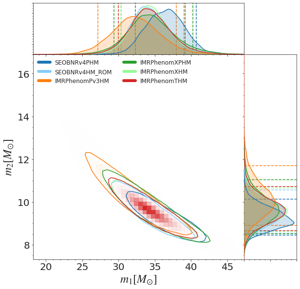
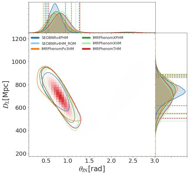
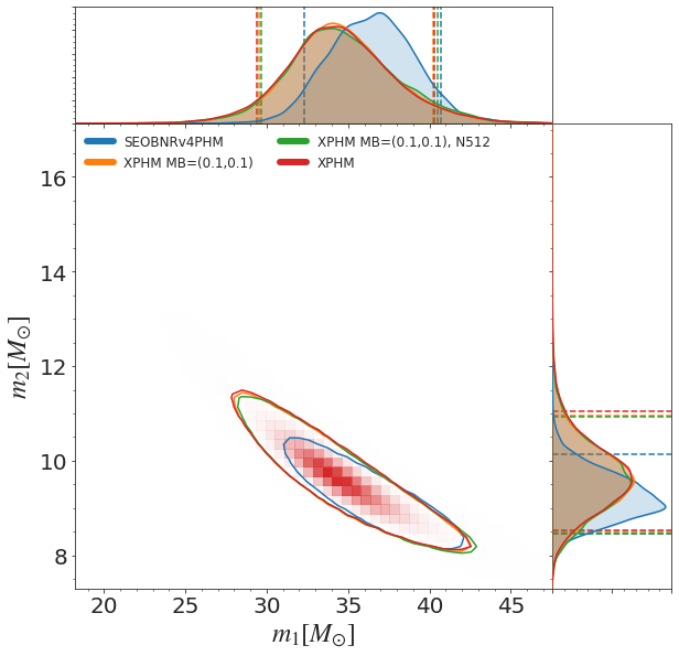
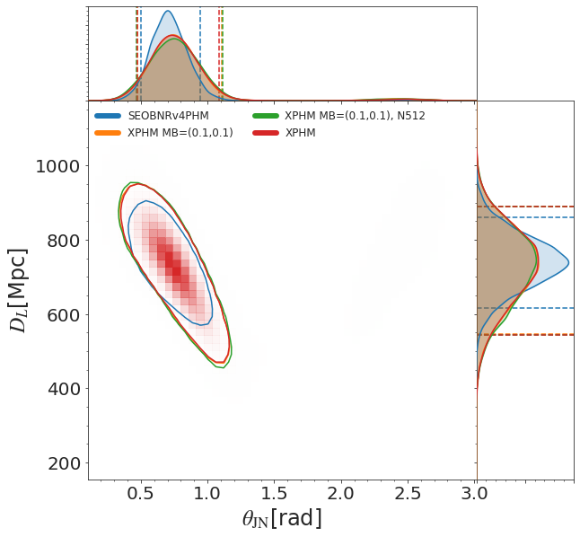
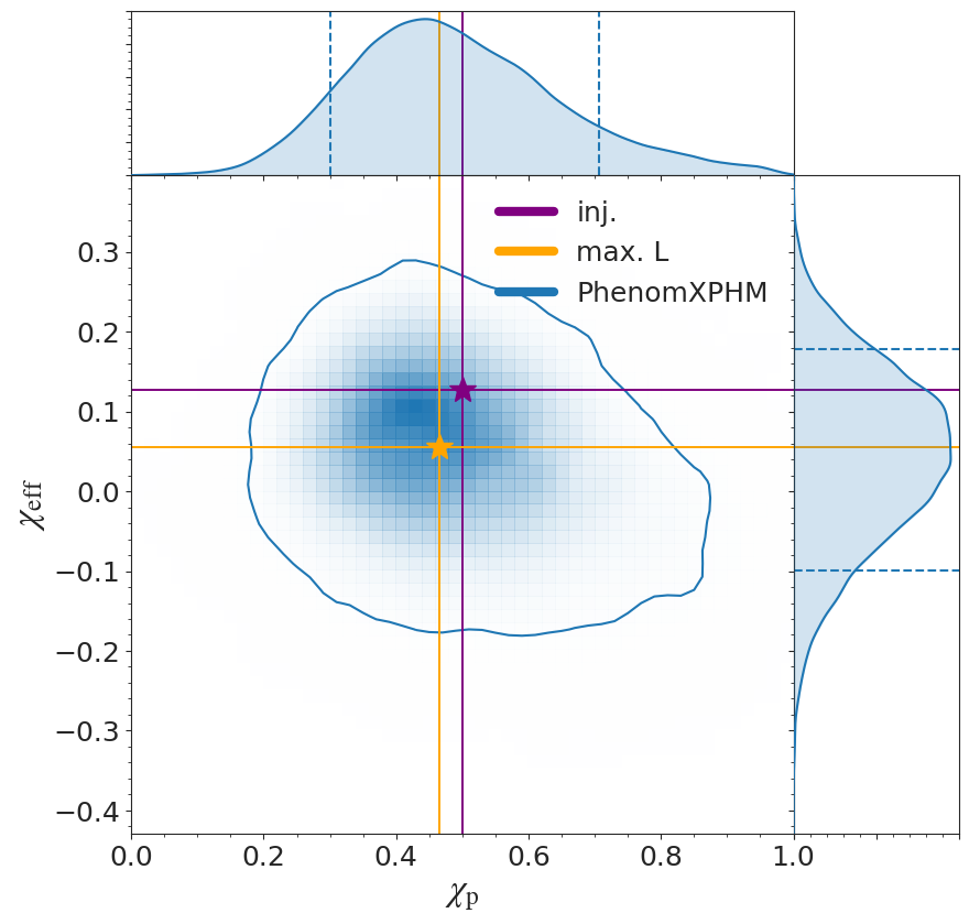
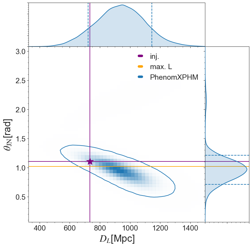
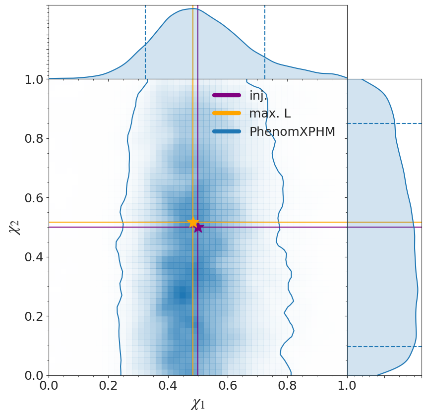
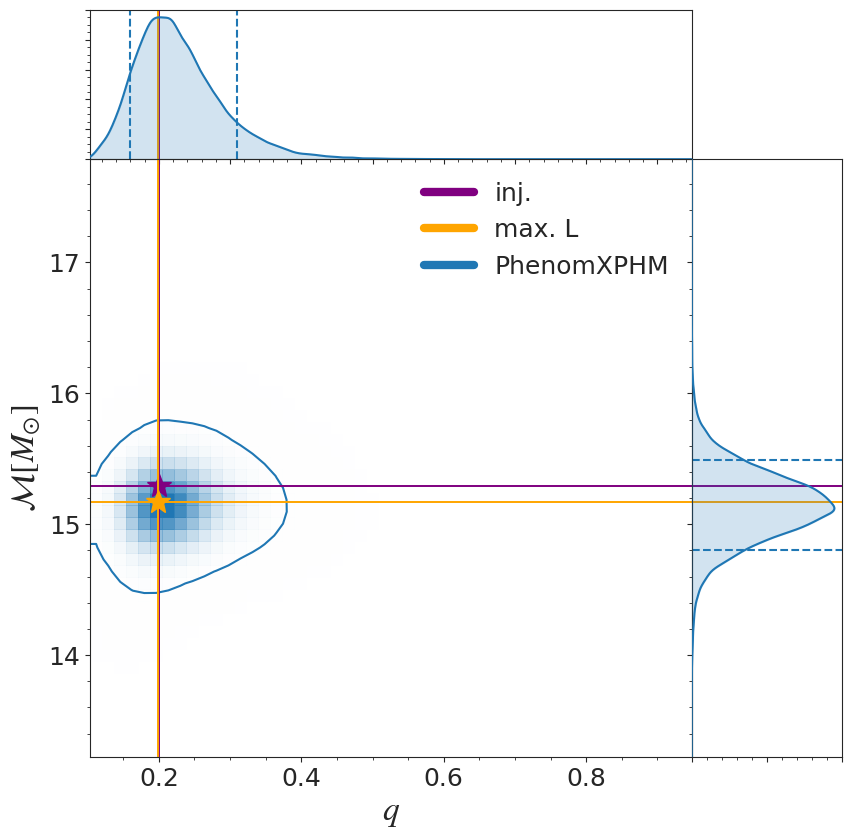
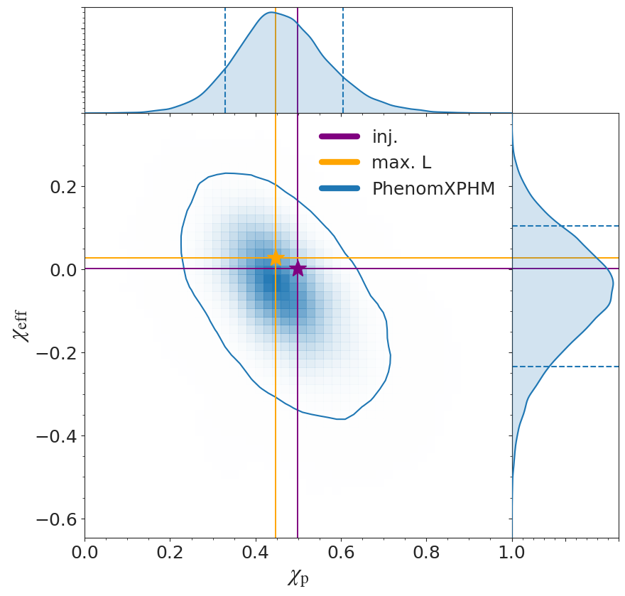
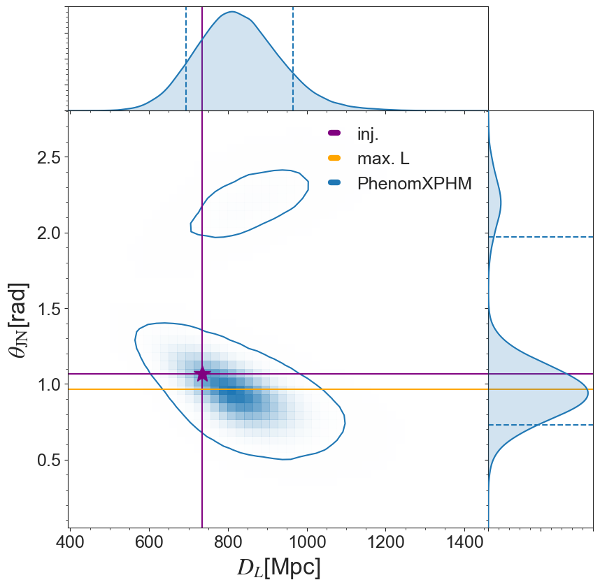
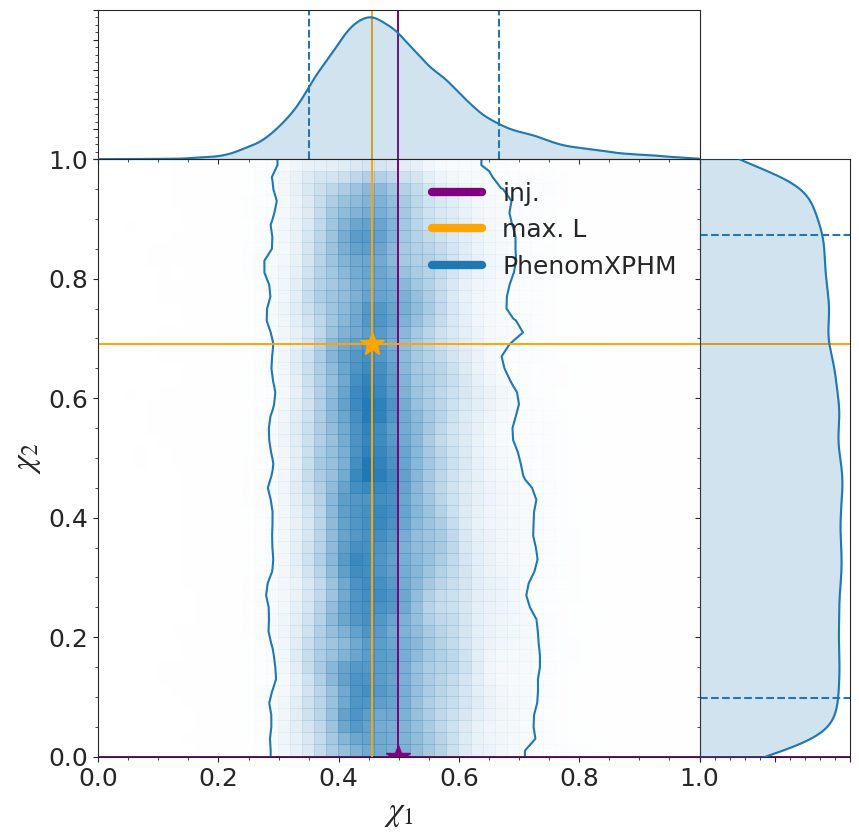
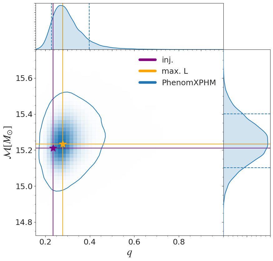
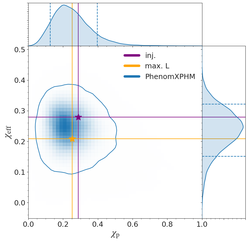
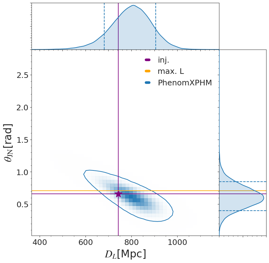
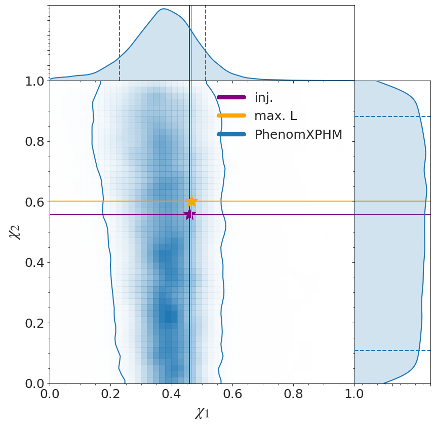
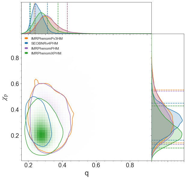
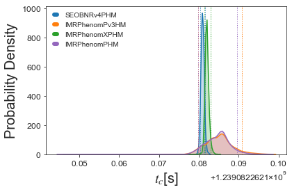
We first compare posterior distributions for the two precessing models used in the LVC paper Abbott et al. (2020a), SEOBNRv4PHM and IMRPhenomPv3HM, with our IMRPhenomXPHM model in Fig. 1. The posterior results for SEOBNRv4PHM and IMRPhenomPv3HM are taken from the official LVC release samples, while those shown for IMRPhenomXPHM correspond to our preferred run (run 26, shown in bold, in Table 3), which uses $n_{\mathrm{live}}=2048$ and $n_{\mathrm{act}}=50$.

Figure 1: Posterior distributions for the masses, effective spin parameters, distance and inclination of GW190412, as estimated with SEOBNRv4PHM (blue), IMRPhenomPv3HM (orange) and IMRPhenomXPHM (green) (using run 26 from Table  3). For each pair of parameters, the square central panel shows the 2D joint posteriors with contours marking 90% credible regions; while the top and right side-panels show one-dimensional distributions for the individual parameters, with dashed lines indicating 90% credible intervals.

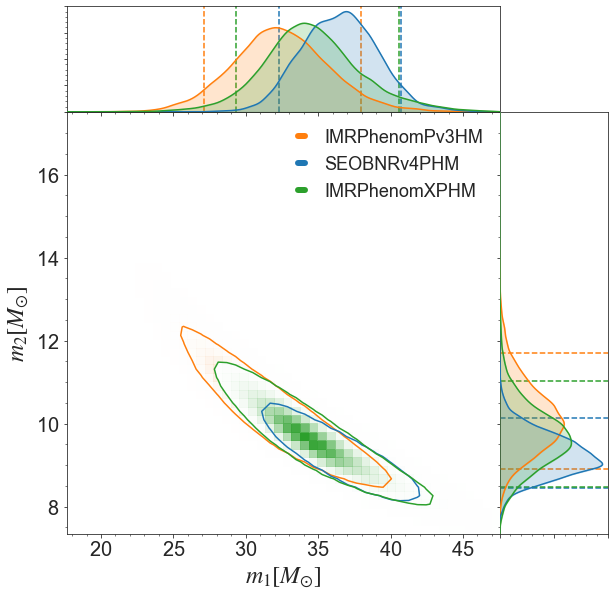
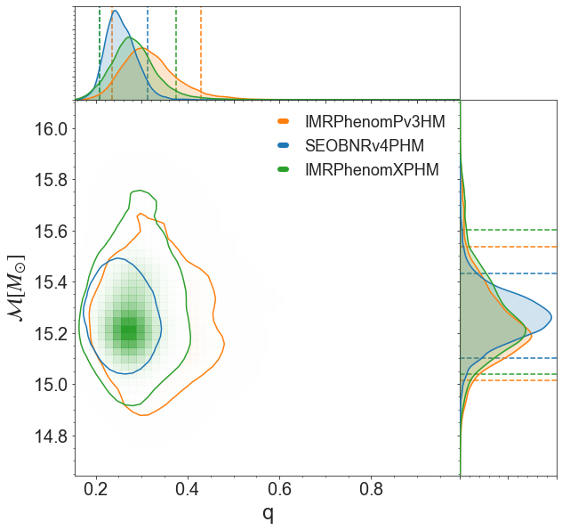
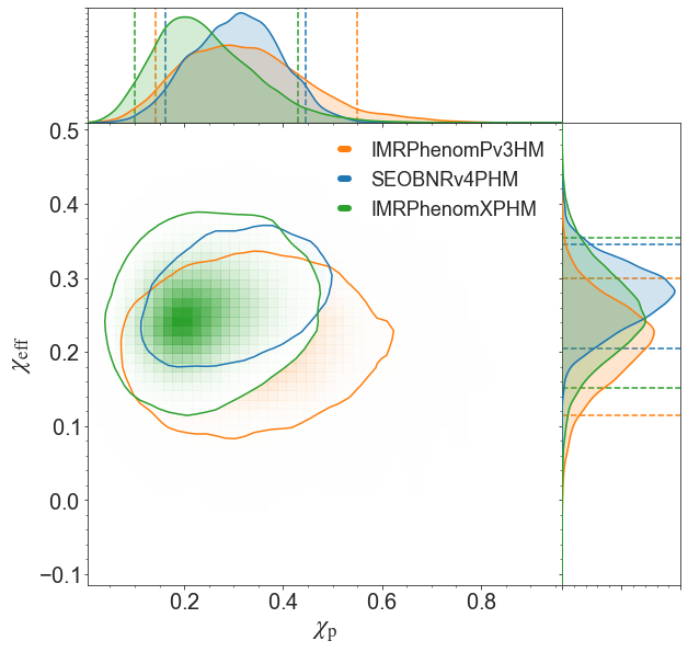
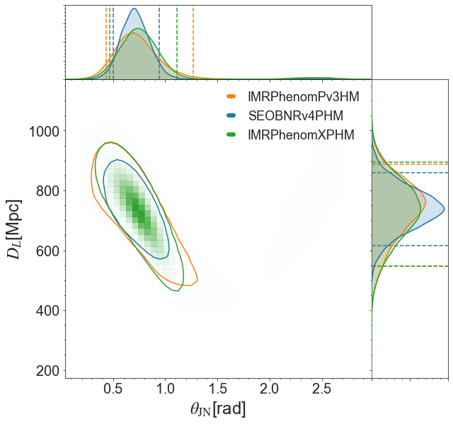
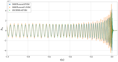
The parameters recovered with the three models considered here are broadly consistent, as can be seen by inspecting the joint posterior distributions for some of the key source properties (Fig. 1) as well as the corresponding maximum-likelihood waveforms (Fig. 2).

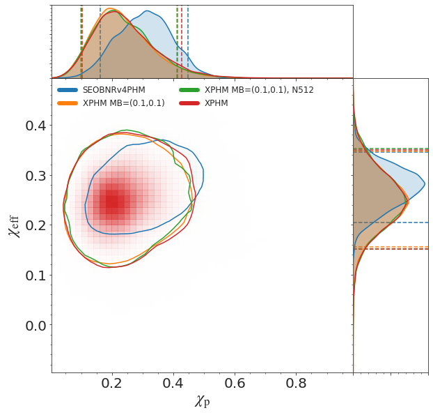
While all these models agree fairly well on the estimated distance and inclination of the source, differences are clearly visible in the mass and spin parameters. The component masses estimated with IMRPhenomXPHM lie in between those estimated with SEOBNRv4PHM and IMRPhenomPv3HM. We notice that IMRPhenomPv3HM tends to return broader posteriors than the other models, which appear to be somewhat more consistent with each other. We also see that SEOBNRv4PHM is favouring more asymmetric masses and higher $\chi_{\mathrm{eff}}$ and $\chi_{\mathrm{p}}$, while IMRPhenomXPHM prefers lower values of $\chi_{p}$, consistently with our analysis of Bayes factors, which will be presented in the next section.

Given the better agreement between the SEOBNRv4PHM and IMRPhenomXPHM models, we compute their combined posterior as our best estimate of the source parameters, and list the estimated source parameters and error estimates in Table 1. These improvements of the LVC estimates which combine SEOBNRv4PHM and IMRPhenomPv3HM posteriors constitute our main astrophysical result.

Figure 2: Waveforms ($h_{+}$ polarization as a function of time) corresponding to the maximum-likelihood samples for IMRPhenomXPHM (blue), IMRPhenomPv3HM (orange) and SEOBNRv4PHM (green). The models show good agreement during the inspiral, while larger differences can be appreciated around merger. The maximum-likelihood sample for IMRPhenomXPHM is taken from run 26.

Figure 3: Comparison of posterior distributions for the component masses, distance and inclination of GW190412, using SEOBNRv4PHM (dark blue), SEOBNRv4_ROM (light blue), IMRPhenomPv3HM (orange), IMRPhenomXPHM (dark green), IMRPhenomXHM (light green) and IMRPhenomTHM (red).

III.2 Comparison with models of reduced content

To investigate support in the GW190412 data for the presence of subdominant modes and precession, we compare a reference run using the full IMRPhenomXPHM model (23 in Table 3) against additional runs with equal sampler settings but using the models IMRPhenomT, IMRPhenomXAS, IMRPhenomXP which drop either one or both of these additional aspects. As discussed above, in fact we called IMRPhenomXHM and IMRPhenomXPHM with $(2,2)$-modes only instead of the named XAS / XP LALSuite approximants.

Our main tool to compare how well each model fits the data are Bayes factors, i.e. ratios of the marginal likelihoods of the models to be compared. If we indicate by $\mathcal{Z}_{A}$ the marginal likelihood of model A and by $\mathcal{Z}_{B}$ that of model B, the Bayes factor will take the form

$$\mathcal{B_{B/A}}=\frac{\mathcal{Z}_{B}}{\mathcal{Z}_{A}},$$ (7)

with $\log_{10}{\mathcal{B}_{B/A}}>1$ indicating that model B is strongly preferred over model A. In Table 4 we list $\log_{10}{\mathcal{B}_{B/A}}$ for two sets of hypotheses, namely whether the signal is best described 1) by an aligned-spin or precessing model and 2) by a quadrupole-only or higher-mode model. Error bars are computed using error propagation, from the uncertainties associated to the evidence integral for each run.

We find strong evidence ($\log_{10}\mathcal{B}>3$) for the presence of higher modes, consistent with the results from Abbott et al. (2020a). On the other hand, there is no actual evidence from the data to infer the presence of precession effects over aligned-only spins, neither when limiting to dominant multipoles or when including the subdominant harmonics. This second result is also consistent with Abbott et al. (2020a) where no numerical $\log_{10}\mathcal{B}$ were reported for this comparison, since they were within numerical and systematic uncertainties – matching our results which are very close to zero.

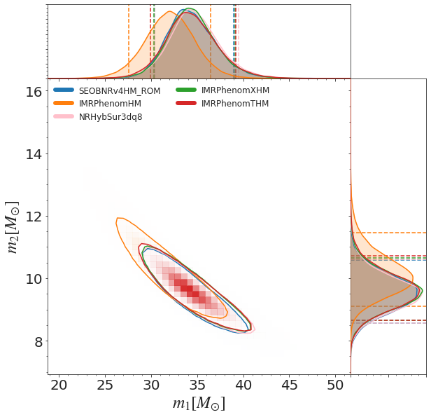
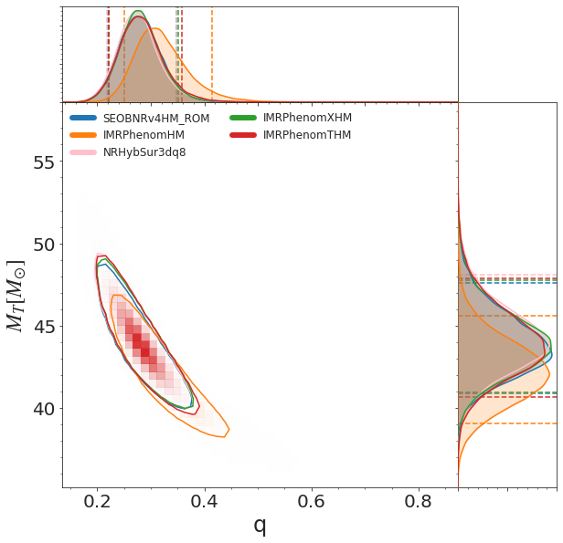
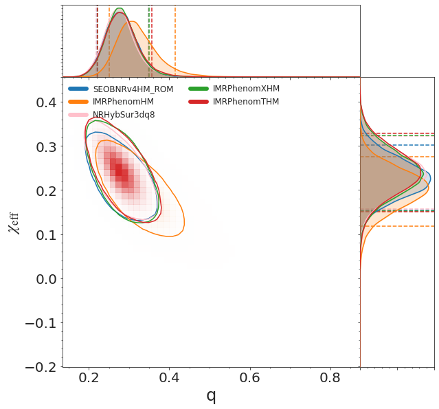
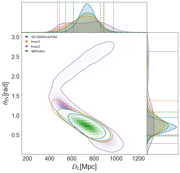
To explore in more detail the differences between the parameters inferred using these models, we compare some of the estimated source parameters for aligned-spin vs precessing models in Fig. 3 and for dominant-mode-only vs. higher-mode models in Fig. 4. One can see here that the inclusion of precession alone does not significantly affect the posterior distributions, while much tighter constraints follow from including higher multipoles, in line with previous studies Shaik et al. (2020); Kumar et al. (2019); Usman et al. (2019). In Fig. 5 we also show comparisons of our own aligned-spin results against those from SEOBNRv4_ROM, NRHybSur3dq8 and IMRPhenomHM, finding excellent agreement with the first two, while IMRPhenomHM is an outlier due to its higher modes not being directly calibrated to NR.

Hypotheses	Model properties	EOB	Phenom	PhenomX	PhenomT
HM vs $\ell=2=|m|$	aligned	3.5	3.4	$3.5\pm 0.1$	$3.4\pm 0.1$
	precessing	4.1	3.6	$3.3\pm 0.1$	-
prec. vs aligned	dominant multipoles	-	-	$0.0\pm 0.1$	-
	higher multipoles	-	-	$0.3\pm 0.1$	-

Table 4: Comparison of Bayes factors $\log_{10}\mathcal{B}$ between EOBNR, Phenom, PhenomX and PhenomT families for two hypothesis tests: (i) whether the signal contains higher or only dominant multipoles, (ii) whether spin precession is present or not. The multipoles test is performed for both aligned and precessing waveforms, and the test for precession both when including only dominant multipoles or also the higher multipoles. No $\log_{10}\mathcal{B}$ numbers are quoted for “prec. vs aligned“ from EOBNR and Phenom because in Abbott et al. (2020a) these were only noted to be not significant in comparison with statistical and systematic error bars.

Figure 4: Comparison of some estimated source parameters, using aligned (pink and purple) and precessing (light and dark green) waveform models from the IMRPhenomX family. Light green and pink correspond to runs where only the quadrupole mode has been activated (note that, for the precessing model, this corresponds to the mode-content in the co-precessing frame). The inclusion of higher multipoles helps to break the degeneracy between distance and inclination, as seen in the plot on the right.

Figure 5: Posterior distributions for the masses, spin parameters, distance and inclination of GW190412, as estimated with aligned-spin waveform models (SEOBNRv4_ROM: blue, NRHybSur3dq8: pink, IMRPhenomHM: orange, IMRPhenomXHM: green, IMRPhenomTHM: red). Models with multipoles individually calibrated to NR (SEOBNRv4_ROM, IMRPhenomXHM and IMRPhenomTHM) are in excellent agreement with the numerical relativity surrogate NRHybSur3dq8, while IMRPhenomHM returns visibly shifted posteriors.

III.3 Contributions from subdominant harmonics

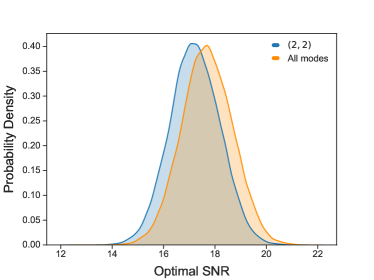
In order to quantify the strength of higher multipoles in GW190412, we consider the posterior samples obtained by analysing the event with IMRPhenomXHM (using run number 5 in Table 3) and compute the SNR distribution corresponding to each mode. The optimal SNR for one mode is defined as

$$\mathrm{\rho^{lm}_{opt}}=\sqrt{(h^{lm}|h^{lm})},$$ (8)

where $(\>|\>)$ refers to the usual noise-weighted inner product

$$(a|b):=\mathrm{Re}\int_{0}^{f_{max}}\frac{\tilde{a}(f)\tilde{b}^{\ast}(f)}{S_{n}(f)}df$$ (9)

and $h^{lm}$ denotes the contribution of a given mode to the strain measured by the detector:

$$h^{lm} =F_{+}h_{+}^{lm}+F_{\times}h_{\times}^{lm},$$ (10)

$$h_{+}^{lm}-ih_{\times}^{lm} =h_{lm}\,{}_{-2}Y_{lm}+h_{l-m}\,{}_{-2}Y_{l-m}.$$ (11)

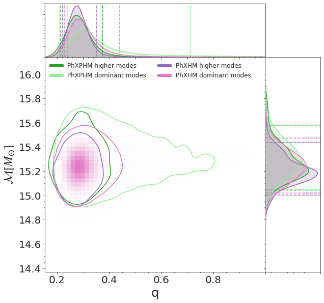
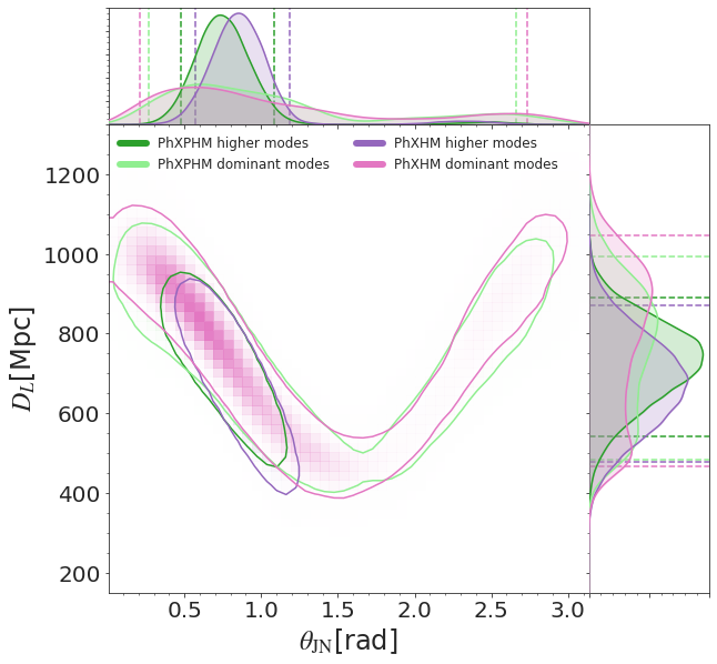
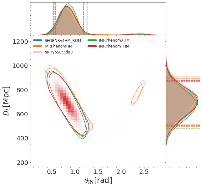
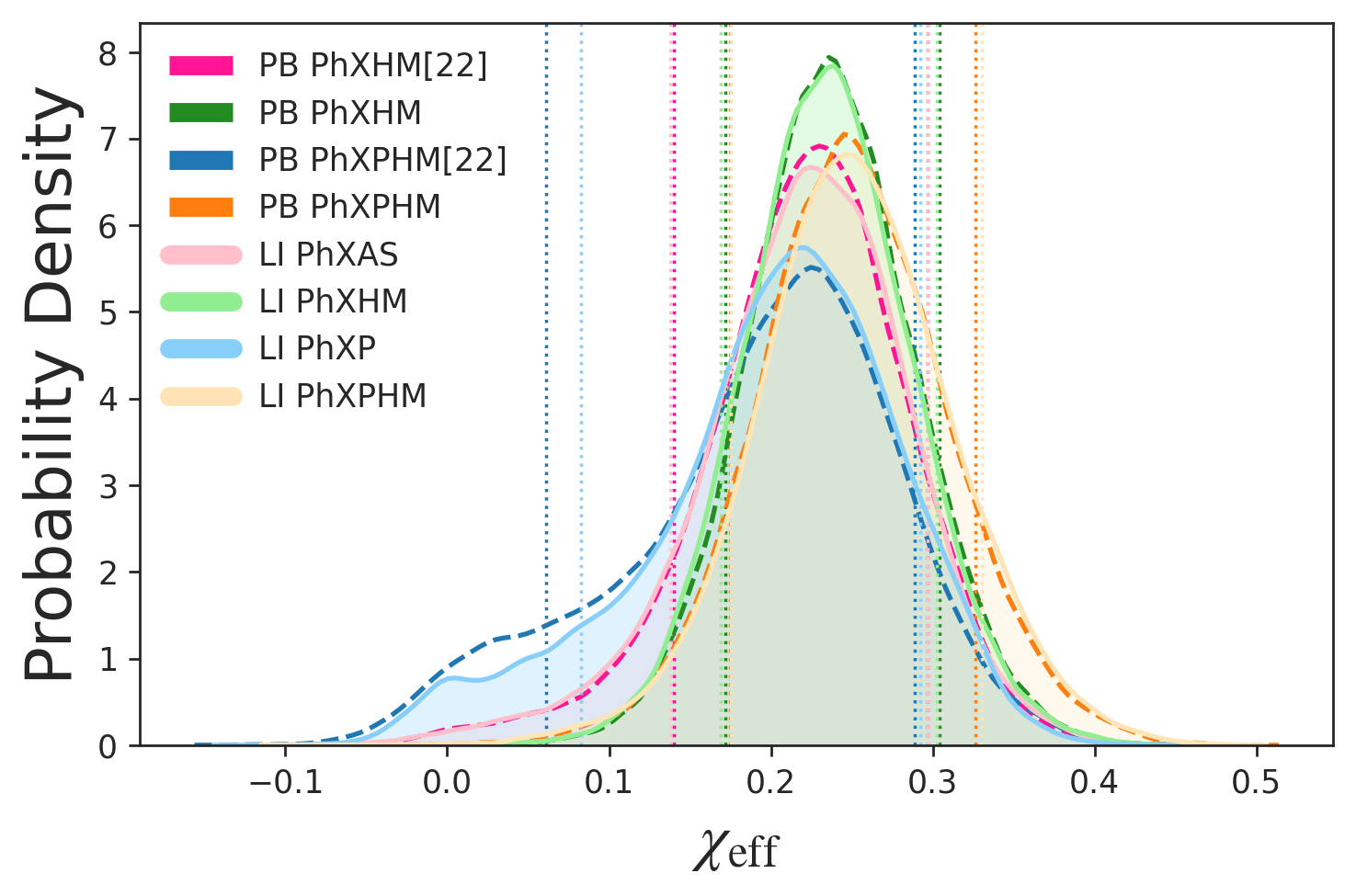
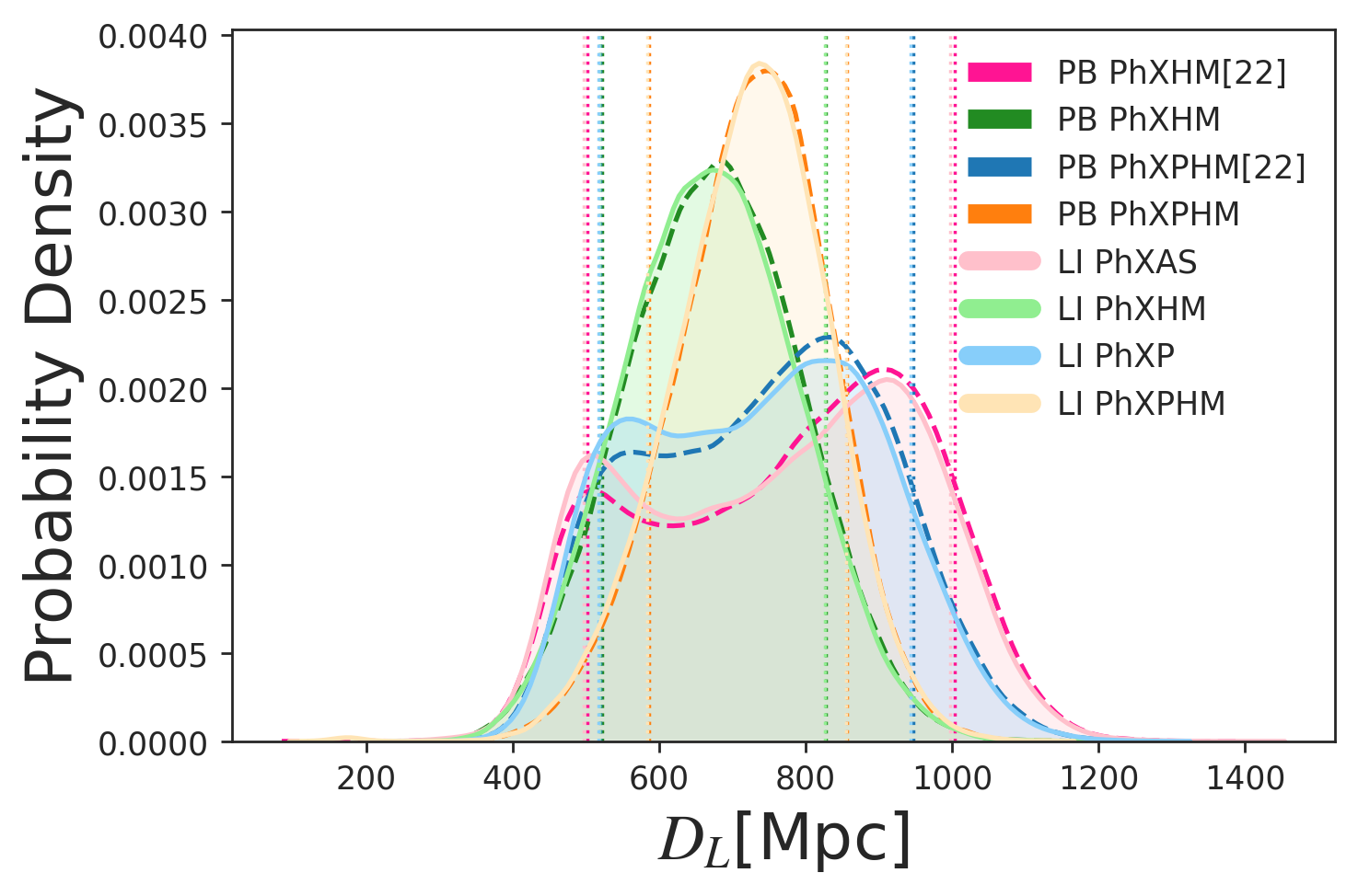
Fig. 6 summarizes our results. In the top panel, we compare the SNR distributions for the subdominant multipoles available in IMRPhenomXHM, and find that the strongest contribution comes from the $(3,3)$ mode, in line with Abbott et al. (2020a) . In the lower panel, we compare the full optimal SNR distribution to that of the quadrupole mode only. As expected, the $(2,2)$ is by far the strongest mode, however, the contribution of subdominant harmonics is clearly non-negligible. This is also illustrated in Fig. 7, where we show the estimated luminosity distance and inclinations obtained when activating only the $\ell=2$ and $\ell\leq 3$ modes and compare them with the results of a standard run, for which $\ell_{\mathrm{max}}=4$. One can clearly see that increasing the mode content of the model results in tighter constraints on the source location. We note also the addition of the $(4,4)$ mode alone, which is the second-strongest subdominant mode, has a visible effect on the posteriors.

Figure 6: Top panel: Optimal SNR distributions for higher multipoles, when recovering the signal with IMRPhenomXHM. The waveform used to compute the SNR contains just one single mode. Bottom panel: SNR distribution for the dominant $(2,2)$ mode only waveform and the whole multimode waveform.

Figure 7: Joint posterior distributions for luminosity distance and inclination of GW190412, as estimated with SEOBNRv4PHM (blue), IMRPhenomXPHM with its full mode-content (green) and IMRPhenomXPHM with only the $\ell=2$ (purple) or $\ell\leq 3$ modes activated.

III.4 Convergence, computational efficiency and cost

One of the main advantages of IMRPhenomXPHM is its computational efficiency, which makes it a potential workhorse for large scale parameter estimation studies, and an ideal tool for convergence tests and systematic studies of sampler settings. This is particularly important considering that future sensitivity improvements of the LIGO-Virgo detector network will result in an increased detection rate Abbott et al. (2018). The modularity of IMRPhenomXPHM, and in particular the possibility to relax the multibanding thresholds, naturally lends itself to a hierarchical PE workflow, where computationally cheap runs can be set up to find optimal choices of priors, while more expensive runs are reserved for final data releases.

Our strategy here has been to select a default configuration with 2048 nested sampling live points ($n_{\mathrm{live}}$) and ($n_{\mathrm{act}}=10$), corresponding to run 23 in Table 3. As we report below, from all our tests this configuration gives robust results when compared both with more expensive settings (increasing $n_{\mathrm{live}}$ and $n_{\mathrm{act}}$), and with computationally cheaper settings. This justifies to use our default setting for comparisons of different choices of precession treatment in appendices C and D, and for comparisons with runs that reduce the physics content in the model to non-precessing spins or the dominant quadrupole in Sec. III.2. We will also show here that configurations with drastically reduced computational cost still reproduce the posteriors of more accurate runs rather well, and are sufficient for fast exploratory runs, e.g. to determine prior settings, or to obtain rapid accurate distance measurements that take advantage of precession and higher harmonics.

Table 3 summarizes all the runs performed with parallel Bilby and distance marginalisation switched on, with different models of the IMRPhenomX family as well as IMRPhenomTHM. Additional parallel Bilby runs without distance marginalisation are listed in Table 8. Most of our runs were performed on IntelXeon Platinum CPUs with 2.1GHz clock-rate (BSC MareNostrum), except for some runs in Table 8, which have been performed on Intel Xeon E5-2670 CPUs with 2.6GHz clock-rate (Picasso machine). All the runs of Table 3 used the master branch of LALsuite, with git hash f253e1307b9c19b0fa974fe627651db483f38170, compiled with gcc version 5.4.0 (BSC MareNostrum) and 4.9.4 (Picasso). The cost of a full higher-mode precessing run with $n_{\mathrm{live}}=2048,n_{\mathrm{act}}=10$ can be as low as $\approx$ 1300 cpu hrs per seed, using aggressive multibanding thresholds and distance marginalization, which translates into a total sampling time of roughly 13 hrs when using 96 CPU-cores. The cost can be further decreased by lowering the number of live points: the fastest run in our analysis, using $n_{\mathrm{live}}=512,n_{\mathrm{act}}=10$ had a computational cost of less than 700 CPU h per seed. We should stress the fact that the computational costs reported here correspond to the analysis of 8 s of data and will be therefore even lower for BBH events with high total masses, for which segment lengths of 4 s are appropriate.

Fig. 8 compares some estimated source parameters obtained with IMRPhenomXPHM, for different combinations of multibanding thresholds and sampler settings. Even for the most aggressive settings, with moderately high multibanding thresholds and $n_{\mathrm{live}}=512$, one cannot appreciate large differences with respect to our default run.

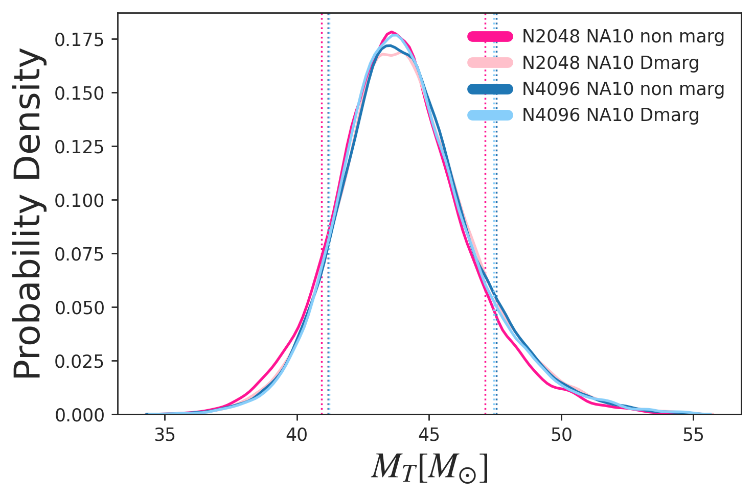
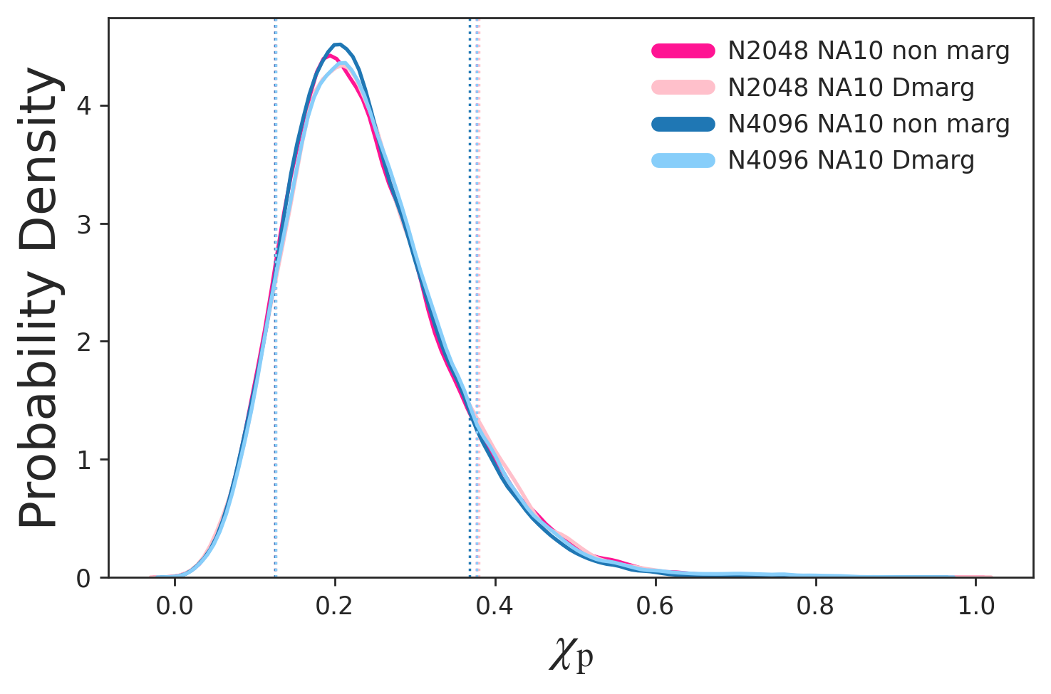
To quantify the robustness of results under changes of sampler settings, we have computed the JS divergences (see definition in Sec. II.4) between IMRPhenomXPHM runs employing different numbers of $n_{\mathrm{live}}$ and/or $n_{\mathrm{act}}$. Our results are summarised in Table 6. For comparison Table 5 lists JS divergences between runs with different models.

Among the divergences of runs with different sampler settings but the same IMRPhenomXPHM model, statistically significant discrepancies (defined as $JS\geq 0.002$, according to the same criterion adopted in Romero-Shaw et al. (2020)), occur more frequently for the cheapest configurations ($n_{\mathrm{live}}=512$), as expected. We also observe that $n_{\mathrm{live}}=2048,n_{\mathrm{act}}=10$ gives already entirely satisfactory results when compared with more expensive settings and could be therefore considered a safe configuration for productions runs on this event.

XAS	-
XHM	$JS_{\phi_{c}}=0.2929$	-
XP	$JS_{t_{1}}=0.6689$	$JS_{t_{1}}=0.6863$	-
XPHM	$JS_{t_{1}}=0.6691$	$JS_{t_{1}}=0.68791$	$JS_{\psi}=0.2659$	-
	XAS	XHM	XP	XPHM

Table 5: Maximum Jensen-Shannon (JS) divergence values between the posterior distributions of GW190412 estimated with IMRPhenomXAS, IMRPhenomXHM, IMRPhenomXP and IMRPhenomXPHM.

N512 NA10	-
N512 NA50	$JS_{t_{1}}=0.0010$	-
N1024 NA10	$JS_{t_{2}}=0.0032$	$JS_{t_{2}}=0.0023$	-
N1024 NA50	$JS_{t_{1}}=0.0008$	$JS_{ra}=0.0007$	$JS_{ra}=0.0019$	-
N2048 NA10	$JS_{ra}=0.0020$	$JS_{ra}=0.0020$	$JS_{t_{2}}=0.0010$	$JS_{ra}=0.0017$	-
N2048 NA50	$JS_{\phi_{JL}}=0.0015$	$JS_{\phi_{JL}}=0.0016$	$JS_{t_{2}}=0.0014$	$JS_{a_{2}}=0.0017$	$JS_{\phi_{JL}}=0.0013$	-
N4096 NA10	$JS_{ra}=0.0023$	$JS_{ra}=0.0027$	$JS_{\theta_{JN}}=0.0030$	$JS_{\theta_{JN}}=0.0018$	$JS_{\theta_{JN}}=0.0033$	$JS_{\theta_{JN}}=0.0020$	-
	N512 NA10	N512 NA50	N1024 NA10	N1024 NA50	N2048 NA10	N2048 NA50	N4096 NA10

Table 6: Maximum Jensen-Shannon (JS) divergence values between the posterior distributions of GW190412 estimated with IMRPhenomXPHM using different sampler settings. In this table, N is short for $n_{\mathrm{live}}$ and NA is short for $n_{\mathrm{act}}$. We report here only values larger than 0.001.

Figure 8: Comparison of some estimated source parameters obtained with SEOBNRv4PHM (blue) and IMRPhenomXPHM, with different combinations of multibanding thresholds and sampler settings (red for the default version, orange with aggressive multibanding thresholds for both the aligned-spin waveforms and precession angles, green with aggressive multibanding and $n_{\mathrm{live}}=512$).

IV Further waveform systematics studies

IV.1 Matches for low total-mass binaries

Waveform systematics can be further investigated by computing noise weighted frequency-domain overlaps between model and signal waveforms:

$$\Braket{h_{\mathrm{M}},h_{\mathrm{S}}}=4\Re\int_{f_{\min}}^{f_{\max}}\frac{\tilde{h}_{\mathrm{M}}(f)\>\tilde{h}^{*}_{\mathrm{S}}(f)}{S_{\mathrm{n}}(f)},$$ (12)

where $S_{\mathrm{n}}(f)$ is the one-sided PSD of the detector noise. In what follows, we will take IMRPhenomXPHM as the model and assume that the signal is given either by a NR or SEOBNRv4PHM waveform. We will quantify the agreement between model and signal by means of the match function:

$$\mathcal{M}(h_{\mathrm{M}},h_{\mathrm{S}})=\max_{t_{c},\phi_{0},\psi_{0}}\frac{\Braket{h_{\mathrm{M}},h_{\mathrm{S}}}}{\sqrt{\Braket{h_{\mathrm{M}},h_{\mathrm{M}}}}\sqrt{\Braket{h_{\mathrm{S}},h_{\mathrm{S}}}}},$$ (13)

where we optimize the overlap between normalized waveforms over polarization angle $\psi_{0}$, coalescence time $t_{c}$ and reference phase $\phi_{0}$. In general, the definition of the spin configuration at the reference frequency will not be the same for the model and the signal. To account for this, we also optimize the match over rotations of the initial in-plane spins. We use the Advanced-LIGO Aasi et al. (2015) design sensitivity Zero-Detuned-High-Power PSD Barsotti et al. (2018) with $f_{\mathrm{min}}=$20 Hz and $f_{\mathrm{max}}=$2048 Hz.

Match calculations are far cheaper than a fully fledged Bayesian analysis and can be leveraged for extensive explorations in parameter space. We extended our previous results Pratten et al. (2020b) and specifically targeted low total-mass binaries similar to GW190412.

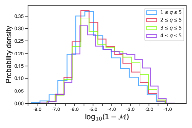
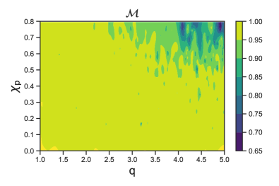
We computed the match between SEOBNRv4PHM and IMRPhenomXPHM waveforms for 20000 random configurations with mass ratios uniformly distributed in the interval $q\in\left[1,5\right]$, spins isotropically distributed on the unit sphere and total mass varying between 30$M_{\odot}$ and 50$M_{\odot}$ in bins of 5$M_{\odot}$ width. Our results are illustrated in Fig. 9. The top panel shows the normalized probability distribution of $\log(1-\mathcal{M})$. Overall, the two models agree very well, with $\approx$ 90% of the configurations achieving $\mathcal{M}\geq 95\%$; however, it can be seen that matches tend to degrade for higher mass ratios. The lower panel shows instead the match $\mathcal{M}$ as a function of the mass ratio $q$ and the effective precession spin $\chi_{\mathrm{p}}$. We notice that the two models can show fairly large disagreement when it comes to strongly precessing, high mass ratio systems.

Figure 9: Matches between IMRPhenomXPHM and SEOBNRv4PHM waveforms. The top panel shows the distribution of mismatches for different ranges in mass-ratio $q$. The lower panel shows the match as a function of the mass ratio $q$ and effective precession spin $\chi_{\mathrm{p}}$. Light green (dark blue) areas indicate good (poor) agreement between the two models. The worst matches correspond to strongly precessing, high mass-ratio binaries.

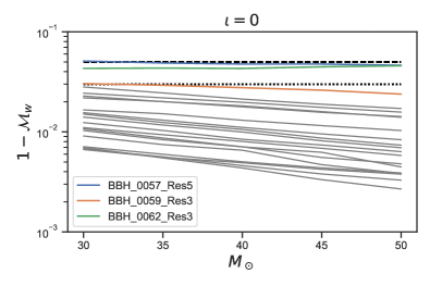
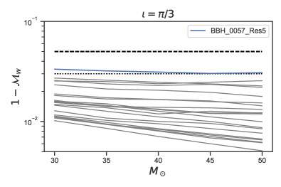
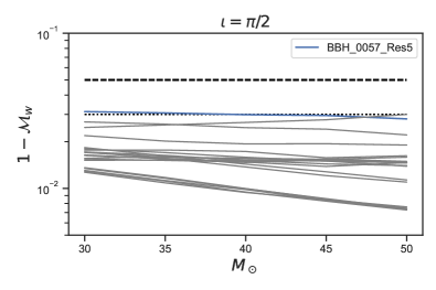
We have also checked the agreement between the model and NR for low total mass binaries. The NR simulations considered here are all public SXS precessing waveforms available in the lvcnr catalog Schmidt et al. (2017). For simplicity, we focused on systems with $q\in[2,5]$, as all the precessing higher mode models considered here tend to exclude mass ratios outside of this range for GW190412. In this case we quantify the agreement between model and signal (NR) through the SNR-weighted match $\mathcal{M}_{\mathrm{w}}$  Harry et al. (2016)

$$\mathcal{M}_{\mathrm{w}}=\left(\frac{\sum_{i}\mathcal{M}_{i}^{3}\Braket{h_{i,\mathrm{NR}},h_{i,\mathrm{NR}}}^{3/2}}{\sum_{i}{\Braket{h_{i,\mathrm{NR}},h_{i,\mathrm{NR}}}^{3/2}}}\right)^{1/3},$$ (14)

where the subscript $i$ goes over different polarization and reference phases of the signal. Fig. 10 shows our results: coloured lines correspond to simulations for which the maximum mismatch $1-\mathcal{M_{\mathrm{w}}}$ is above 3% in the mass range considered. The three outliers with mismatches above this threshold are SXS:0057, SXS:0059 and SXS:0062, which all correspond to $q=5$ binaries. These result confirm the conclusions drawn in Pratten et al. (2020b). Overall, SEOBNRv4PHM and IMRPhenomXPHM show good agreement over most of the parameter space and are expected to deliver comparable estimates for typical BBH events. However, exceptional events with very asymmetric masses and/or strong precession might require a more in-depth analysis, which we leave for future work. Further insight on waveform systematics can be found in previous works on the IMRPhenomX family models Pratten et al. (2020a); García-Quirós et al. (2020, 2020); Pratten et al. (2020b) where extensive comparisons through matches with previous waveform models and NR simulations are carried out.

Figure 10: SNR-weighted mismatches between IMRPhenomXPHM and precessing SXS waveforms with $q\in[2,5]$. The dotted and dashed lines in each panel denote thresholds of 3% and 5%, respectively. Cases for which the maximum mismatch exceeds the 3% threshold are shown with coloured lines and listed in the legends.

IV.2 Injection study

In order to assess the accuracy of our measurements, in particular of the precessing spin, we injected into a Hanford-Livingston-Virgo detector network three synthetic signals and recovered their parameters with IMRPhenomXPHM. Two of these signals are based on NR simulations with moderately high $\chi_{p}$, while the third one makes use of a SEOBNRv4PHM waveform, corresponding to the maximum-likelihood sample of the LVC release. We injected the signals in zero noise, but we fed into the likelihood estimation the PSDs used to analyse GW190412. For the NR signals, the total mass and luminosity distance were chosen so as to achieve a network SNR comparable to that of GW190412. In all cases, we set the reference frequency to be the same as the minimum frequency, i.e. $f_{\mathrm{ref}}=f_{\mathrm{low}}$ in our setup.

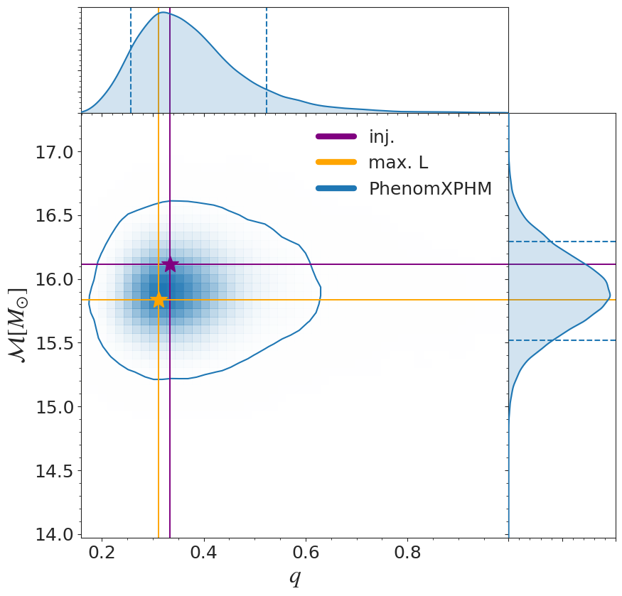
The first injection made use of the public NR waveform SXS:BBH:0049, corresponding to a $q=3$ binary with $\chi_{\mathrm{p}}\approx 0.5$. We simulated a binary with right ascension ra$=3.81$ rad, declination dec$=0.63$ rad, and geocentric time equal to the trigger time reported in GraceDB LIGO Scientific Collaboration and Virgo Collaboration (2020). We used a minimum frequency of 25.7 Hz, due to the limited length of the NR waveform. In Fig. 11 we present posteriors for detector-frame masses, $\chi_{\mathrm{eff}}$, $\chi_{\mathrm{p}}$, luminosity distance, $\theta_{\mathrm{JN}}$, as well as the individual adimensional spin magnitudes $a_{1}$ and $a_{2}$. Overall, we observe a very good agreement between the recovered parameters and the injected values, which always lie within the $90\%$ credible intervals of the posterior distributions. In particular, the spin magnitude of the primary is very well constrained, similarly to what happens for GW190412.

Figure 11: Posterior distributions for some of the intrinsic and extrinsic parameters of a synthetic signal obtained starting from the public SXS waveform SXS:BBH0049. Purple and orange stars mark the values of the injected and maximum-likelihood parameters, respectively. Dashed lines indicate the $90\%$ credible intervals of the individual posterior distributions.

In Fig. 12 we present the results of our second NR injection, that took as input the public SXS waveform SXS:BBH0058, corresponding to a $q=5$ binary with $\chi_{\mathrm{p}}\approx 0.5$. The simulated event was assumed to have the same celestial coordinates and geocentric time as the previous mock signal. The total mass of the system was taken to be $50.5M_{\odot}$ in the detector frame, and we used a minimum frequency of 20.5 Hz. We can see that, even in this case, all the recovered parameters are consistent with the ones of the injected signal.

Figure 12: Posterior distributions for some of the intrinsic and extrinsic parameters of a synthetic signal obtained starting from the public SXS waveform SXS:BBH0058. Purple and orange stars mark the values of the injected and maximum-likelihood parameters, respectively. Dashed lines indicate the $90\%$ credible intervals of the individual posterior distributions.

Finally, we injected in zero-noise the maximum-likelihood waveform for the SEOBNRv4PHM sample. The injected signal had a total mass of $46.66M_{\odot}$ in detector frame, celestial coordinates $\mbox{ra}\approx 3.81$ rad and $\mbox{dec}\approx 0.64$ rad, and geocentric time of approximately $1239082262.18$ s. Fig. 13 summarizes our main results. IMRPhenomXPHM recovers well all the parameters of the injected signal. We therefore conclude that IMRPhenomXPHM appears to deliver robust estimates of the source properties for events similar to GW190412.

Figure 13: Posterior distributions for some of the intrinsic and extrinsic parameters of a synthetic signal obtained from the SEOBNRv4PHM maximum-likelihood parameters for GW190412. Purple and orange stars mark the values of the injected and maximum-likelihood parameters, respectively. Dashed lines indicate the $90\%$ credible intervals of the individual posterior distributions.

V Conclusions

We have re-analysed the event GW190412 with the newest generation of phenomenological waveform models: the frequency-domain model IMRPhenomXPHM, which includes precession and higher modes, and the time-domain model IMRPhenomTHM, which includes higher modes, but not yet precession. Both models have been constructed with similar techniques and accuracy goals, and we refer to them (and several versions with reduced physics content) jointly as “generation X”.

The principal code we have used for performing Bayesian inference is parallel Bilby Smith et al. (2019), which allows us to work in traditional high performance computing environments and to obtain results on a time scale of hours. In Sec. III.4 we have described some tests varying sampling parameters to convince us that our parallel Bilby runs have converged to reliable results. In appendix B we further test that our main runs, which use distance marginalisation, agree with runs that do not use it, and we study the difference in the number of likelihood evaluations and computational cost. Since parallel Bilby is a relatively new code, we also report our cross-checks with the more established LALInference code Veitch et al. (2015) in appendix A, and find excellent agreement.

For the non-precessing sector, we find excellent agreement between all waveform models where sub-dominant harmonics have been calibrated to numerical waveforms, i.e. SEOBNRv4HM, NRHybSur3dq8, IMRPhenomXHM and IMRPhenomTHM (see e.g. Fig. 5). However we find significant differences for IMRPhenomHM, where higher modes have been constructed by an approximate map in terms of the dominant quadrupole mode, which was calibrated to a much smaller set of NR waveforms than IMRPhenomXAS. It is to be expected that in the future, EOB and phenomenological models will also be calibrated to numerical relativity waveforms for the precessing sector, and will thus reach similar levels of agreement.

When adding precession we find that the agreement between phenomenological waveforms and the EOB model improves for some quantities, notably the masses and source location. Not surprisingly, for the effective precession spin this is not the case, although the posterior width for IMRPhenomXPHM is closer to SEOBNRv4PHM than IMRPhenomPv3HM. Both SEOBNRv4PHM and the frequency-domain phenomenological waveforms use a version of the “twisting-up” approximate map between non-precessing and precessing waveforms Hannam et al. (2014), however the current frequency domain phenomenological waveforms employ the stationary phase approximation (SPA) in addition to the approximations inherent in the twisting-up (for a recent discussion of these approximations see Ramos-Buades et al. (2020)). An improved accuracy for precession is thus expected from the extension of the LALSuite implementation of IMRPhenomT to include precession following Estellés et al. (2020). Strategies for extending the twisting-up procedure for frequency-domain waveforms beyond the SPA approximation have been discussed in Marsat and Baker (2018). In appendix C we compare the two different descriptions of the Euler angles used in the twisting-up procedure implemented in IMRPhenomXPHM (single-spin and double-spin), and only find small differences, mainly in the effective precession spin parameter $\chi_{p}$. Not surprisingly we find that the double-spin description is closer to the results that have been reported for SEOBNRv4PHM in Abbott et al. (2020c). In the same section we also compare different prescriptions for the spin of the merger remnant in precessing mergers, and we find no significant differences for GW190412. In appendix D we compare directly against an alternative “twisting-up” of the older IMRPhenomHM aligned-spin model implemented within the IMRPhenomXPHM framework, finding consistent results with the original IMRPhenomPv3HM (which is based on IMRPhenomHM), thus cleanly demonstrating that our improved results mostly derive from the updated underlying aligned-spin model IMRPhenomXHM with its calibration of subdominant modes to NR. We have also shown that the use of the multibanding algorithm leads to a dramatic reduction of the computational cost of parameter estimation runs, nearly halving the cost of non-multibanded runs.

Additional studies presented in this paper include investigations into possible remaining systematic differences between waveforms, including waveform match comparisons and injection studies in Sec. IV. The tested injections include SXS waveforms with parameters consistent with GW190412 as well as the SEOBNRv4PHM maximum-likelihood waveform, finding no significant systematic issues with IMRPhenomXPHM in this part of the parameter space. We also test the impact of different spin priors in appendix E, finding that PE results for GW190412 are generally consistent when changing from the standard LVC prior to a volumetric one, and confirming the results of Zevin et al. (2020) that the standard assumption of allowing for a spinning heavier BH component is preferred over runs with a prior that restricts spin to the less massive BH only.

One of the key properties of the IMRPhenomX waveform family is its computational efficiency. We demonstrate that even the most complete IMRPhenomXPHM model, when making use of the pBilby sampler and a strong HPC cluster, allows for extremely fast-turn-around exploratory runs (few hours) and still very fast high-fidelity runs like the ones we report as the main results (see e.g. Fig. 1, with the plotted IMRPhenomXPHM run taking 2670 CPU hours total and finishing after 28 hours wall-clock time). The time-domain IMRPhenomTHM model is also quite competitive in run time despite being a native time domain model, having only 50 more CPU cost per likelihood evaluation than IMRPhenomXHM. More details on computational cost for different model versions and sampler settings are found in Table 3 (for the runs with distance marginalization) and Table ,8 (for the runs without distance marginalization). As expected, the use of distance marginalization brings significant computational cost savings: this can be readily appreciated by comparing otherwise equivalent runs from the two tables (e.g. run 23 in Table 3 and run 20 in Table 8).

In summary, the studies presented here demonstrate the robustness and efficiency of the “generation X” phenomenological waveform models in a real-world application, and point out how systematic runs with varied settings can be used both to study the physics of an individual detection in detail, and to achieve accuracy requirements at bounded computational cost. We hope these results will help to advance the routine use of subdominant harmonics in the parameter estimation for compact binary mergers, leading to both more accurate parameter estimates, and the availability of accurate posterior estimates on the time scale of a few hours.

Posterior samples from our preferred run for each waveform model are released in Colleoni et al. (2020).

Appendix A Comparison between pBilby and LALInference

In order to cross-validate our parallel Bilby results, we perform the runs listed in Table 7 using the Bayesian parameter estimation package LALInference (LI) Veitch et al. (2015). The runs that make use of nested sampling employ five different seeds, 2048 live points, and a maximum chain length of 5000. Those that use MCMC sampling, utilize eight parallel tempering temperatures and 24 parallel chains.

In Fig. 14 we compare the standard runs of Table 3 using $n_{\mathrm{live}}=2048$ and $n_{\mathrm{act}}=10$ (dashed) with the default LI runs (solid). All posteriors are well recovered, and we find generally good agreement between pBilby and LI runs. We also observe that the agreement is better in the presence of higher modes. A possible explanation is that the breaking of degeneracies due to higher modes reduces the posterior volume and thus benefits better sampling.

Approximant	Run $nº$	Modes (l,|m|)	PV	FS	PMB	MB	Prior	Sampler	nlive	max. mcmc	nparallel	ntemps
IMRPhenomXAS	1	(2,2)	-	-	-	-	Aligned spin	Nested	2048	5000	5	-
IMRPhenomXHM	2	D	-	-	-	D	Aligned spin	Nested	2048	5000	5	-
IMRPhenomXP	3	(2,2)	D	D	D	D	Precessing	Nested	2048	5000	5	-
	4	(2,2)	102	D	D	D	Precessing	Nested	2048	5000	5	-
IMRPhenomXPHM	5	D	D	D	D	D	Precessing	MCMC	-	-	24	8
	6	D	102	D	D	D	Precessing	MCMC	-	-	24	8
	7	D	102	D	D	D	Precessing	Nested	2048	5000	5	-

Table 7: List of all LALInference runs we performed on open data for GW190412 using the IMRPhenomX family. For each run, we indicate the LALSuite waveform approximant called along with along with various waveform settings: the mode content, precessing prescription (PV), final spin version (FS), and multibanding thresholds applied to the evaluation of the Euler angles (PMB) and of the aligned-spin modes (MB); as well as the prior used. We also denote the sampler used (Nested or MCMC) and its corresponding settings such as number of live points (nlive), maximum chain length (max. mcmc), parallel chains (nparallel) and the number of parallel tempering temperatures (ntemps).

Figure 14: Posterior distributions of several source parameters comparing the LALInference (LI) runs as listed in Table 7 (solid) and the standard parallel Bilby runs from Table 3 using $n_{\mathrm{live}}=2048$ and $n_{\mathrm{act}}=10$ (dashed).

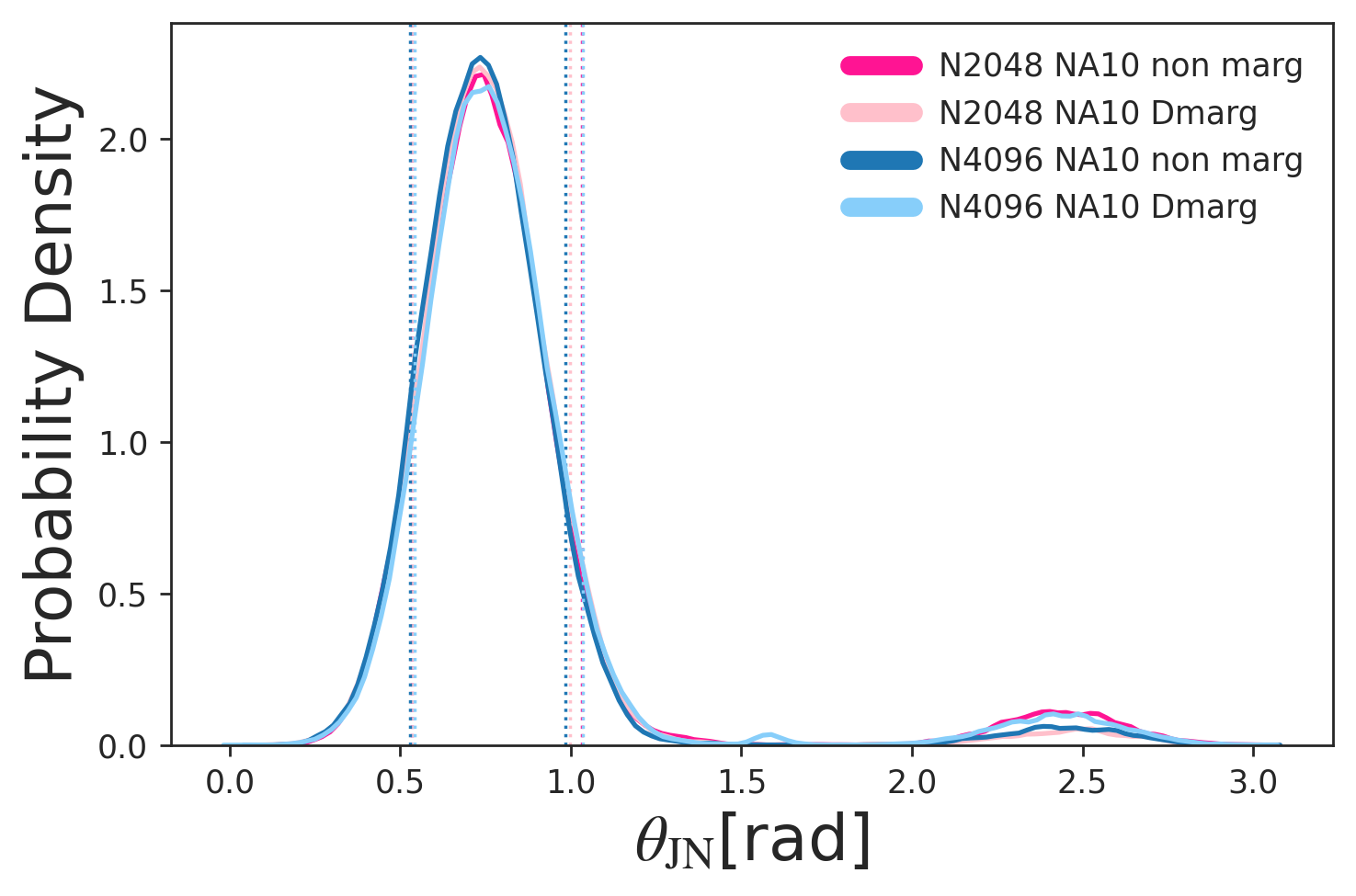
Appendix B Comparison of runs with and without distance marginalisation

We report in Table 8 the complete list of pBilby runs performed on GW190412 without using distance marginalisation (prior to a bugfix in the distance marginalisation algorithm). We find excellent agreement and show a comparison in Fig. 15 for some key quantities.

Approximant	Run $nº$	Modes (l,|m|)	PV	FS	PMB	MB	Prior	$n_{\mathrm{live}}$	$n_{\mathrm{act}}$	CPU h	L. eval.	Cost/L. eval. [ms]
IMRPhenomXAS	1	(2,2)	-	-	-	-	Aligned spin	2048	20	2650	$2.23\times 10^{8}$	42.77
IMRPhenomXHM	2	D	-	-	-	D	Aligned spin	2048	20	4734	$2.90\times 10^{8}$	58.67
IMRPhenomXP	3	(2,2)	102	0	-	-	Precessing	2048	5	1042	$6.57\times 10^{7}$	57.13
	4	(2,2)	D	D	-	-	Precessing	2048	5	1273	$6.32\times 10^{7}$	72.45
IMRPhenomXPHM	5	D	D	D	D	D	Precessing	512	5	1566	$1.99\times 10^{7}$	283.60
	6	D	D	D	D	D	Precessing	1024	5	1531	$3.61\times 10^{7}$	152.55
	7	D	D	D	D	D	Precessing	1024	20	3362	$1.31\times 10^{8}$	92.16
	8	D	D	D	D	D	Uniform $m_{1}$-$m_{2}$	1024	30	7082	$2.05\times 10^{8}$	124.17
	9	D	D	D	D	D	Uniform $m_{1}$-$m_{2}$	1024	50	8362	$3.34\times 10^{8}$	90.10
	10	D	D	D	D	D	Precessing	1024	60	3696	$1.68\times 10^{8}$	79.33
	11	D	D	D	D	D	Precessing	1500	50	5041	$2.31\times 10^{8}$	78.43
	12	D	D	D	D	D	Precessing	2048	5	1804	$7.15\times 10^{7}$	90.85
	13	D	D	D	$10^{-2}$	D	Precessing	2048	5	1295	$7.19\times 10^{7}$	64.85
	14	D	D	D	$10^{-2}$	D	Precessing *	2048	5	1690	$7.18\times 10^{7}$	84.73
	15	D	102	2	D	D	Precessing	2048	5	1336	$7.09\times 10^{7}$	67.83
	16	D	102	0	D	D	Precessing	2048	5	1354	$7.10\times 10^{7}$	68.61
	17	D	223	2	D	D	Precessing	2048	5	1732	$7.24\times 10^{7}$	86.13
	18	No $(3,2)$	D	D	D	D	Precessing	2048	5	1465	$7.21\times 10^{7}$	73.11
	19	D	D	D	D	D	Volumetric spin	2048	5	2216	$7.77\times 10^{7}$	102.68
	20	D	D	D	D	D	Precessing	2048	10	4275	$1.54\times 10^{8}$	99.44
	21	D	D	D	D	D	Precessing	2048	20	6795	$2.66\times 10^{8}$	91.79
	22	D	D	D	D	D	Uniform $m_{1}$-$m_{2}$	2048	30	9070	$4.22\times 10^{8}$	77.25
	23	D	D	D	D	D	Precessing	4096	5	3434	$1.46\times 10^{8}$	84.47
	24	D	D	D	D	D	Precessing	4096	10	6377	$2.89\times 10^{8}$	79.43
	25	D	102	D	D	D	Precessing	4096	10	5132	$2.85\times 10^{8}$	64.75
	26	D	D	D	D	D	Precessing	4096	20	11438	$5.71\times 10^{8}$	72.08
	27	D	D	D	D	D	Uniform $m_{1}$-$m_{2}$	4096	30	20187	$9.49\times 10^{8}$	76.57
	28	D	D	D	D	D	Precessing	8192	5	8921	$2.95\times 10^{8}$	108.94
	29	D	D	D	D	D	Precessing, $\chi_{1}=0$	2048	5	1863	$6.95\times 10^{7}$	96.47
	30	D	D	D	D	D	Aligned, $\chi_{1}=0$	2048	5	1726	$6.31\times 10^{7}$	98.40

Table 8: List of the runs performed on GW190412 open data with parallel Bilby without distance marginalisation, using different models of the IMRPhenomX family. For each run, we indicate the LALSuite waveform approximant called along with various waveform settings: the mode content, precessing prescription (PV), final spin version (FS), and multibanding thresholds applied to the evaluation of the Euler angles (PMB) and of the aligned-spin modes (MB); as well as the prior used and the chosen sampler settings ($n_{\mathrm{live}}$ and $n_{\mathrm{act}}$). We also provide the computational cost of each run, the number of likelihood evaluations and the mean cost of each evaluation. We use 4kHz GWOSC data for all runs in this table, except for the one marked with an asterisk, which employs 16kHz data.

Figure 15: Comparison between some key posterior distributions obtained with and without distance marginalisation, using two sets of sampler settings ($n_{\mathrm{live}}=2048$ and $n_{\mathrm{act}}=10$ vs. $n_{\mathrm{live}}=4096$ and $n_{\mathrm{act}}=10$).

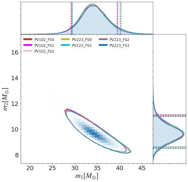
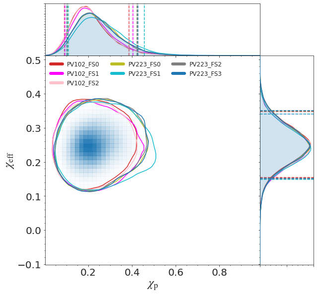
Appendix C Comparison of IMRPhenomX precession and final spin versions

We have performed several IMRPhenomXPHM runs with non-default waveform options to study the robustness of our results under changes of the precession prescription and final spin version. We compare posterior distributions for the default and non-default runs in Fig. 16. Mass parameters appear to be insensitive to changing these settings, while we observe minor differences in the spin parameters, with the MSA prescription returning slightly broader posteriors.

Figure 16: 1D and 2D posterior distributions for detector-frame masses and spin parameters of GW190412 obtained with three versions of IMRPhenomXPHM that implement different precessing prescriptions (102 for NNLO angles and 223 for MSA) and final spin formulae (FS0, FS2, FS3, see main text for more details). The two NNLO results are plotted in red (FS0) and purple (FS2), while the default MSA results is plotted in green. Dashed (solid) lines in the 1D (2D) plots indicate 90% credible intervals (regions).

Appendix D Comparison with IMRPhenomPv3HM

As we observed in the previous subsection, there are visible differences in the posterior distributions obtained with IMRPhenomPv3HM and IMRPhenomXPHM. We mean to quantify here the effect of the underlying aligned-spin model on those results. This can be easily done with IMRPhenomXPHM, which has an in-built option allowing to twist-up the GW modes returned by the older model IMRPhenomHM (we will refer to this configuration as “IMRPhenomPHM”) instead of IMRPhenomXHM. Using this option, one can cleanly separate the effects of the HM calibration from all the details of the precessing extension. Fig. 17 compares previous results with the IMRPhenomPHM run described above.

Figure 17: Left panel: 1D and 2D posterior distributions for the mass ratio and precession spin of the signal recovered with IMRPhenomPv3HM (orange), SEOBNRv4PHM (blue), IMRPhenomXPHM in its default version (green) and its “IMRPhenomPHM” version (purple, see main text for details). Dashed (solid) lines indicate 90% credible intervals (regions). Right panel: posterior distributions for the geocentric time of the event, as estimated with the same models shown in the top panel.

It can be seen that the shifts observed in the posteriors can be ascribed to the different underlying aligned-spin models, as, despite the use of independent precessing extensions, IMRPhenomPv3HM and IMRPhenomPHM return equivalent results. Comparing both against the default IMRPhenomXPHM, we observe in particular a marked difference in the recovery of the geocentric time of the event, due to the improved time-alignment provided by the IMRPhenomX models.

Appendix E Investigating different spin priors

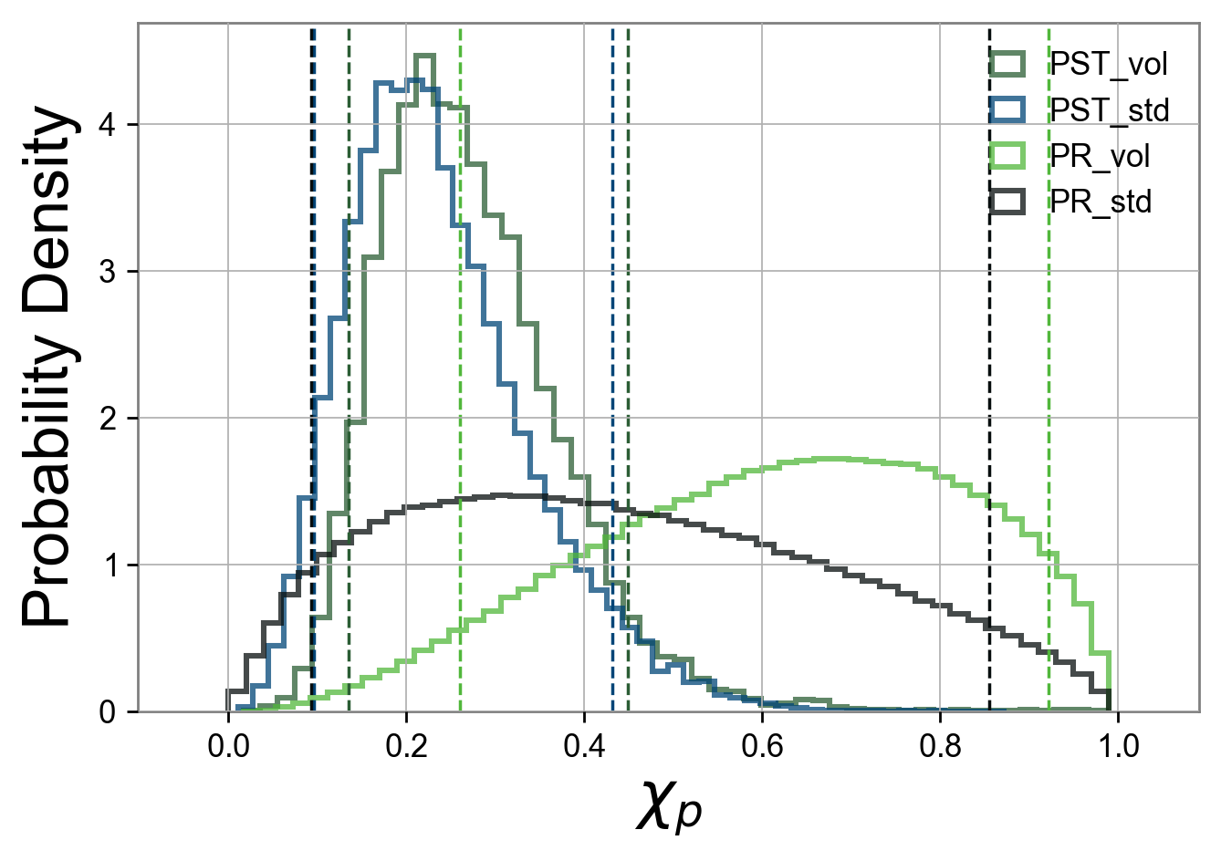
For the vast majority of our runs we adopted the same priors employed in the LVC analysis Abbott et al. (2020a). Specifically, we choose uniform priors for detector-frame mass ratio $0.125\leq q\leq 1$ and chirp mass $13\leq\mathcal{M}\leq 18$, with masses constrained to lie in the interval $5\leq m_{1,2}\leq 60$. We use a power law prior with exponent 2 for the luminosity distance, with a lower bound of 100 Mpc and uniform priors for phase and polarization angle. We also investigate the effect of different spin priors on the posterior estimates, in particular on the $\chi_{\mathrm{p}}$ parameter whose interpretation is subtle. Our default prior for precessing runs, in keeping with the LVC standard (defined as prior “P1" in appendix C.1 of Abbott et al. (2019a) and also used in the analysis of GW190412 Abbott et al. (2020a)), employs uniform distributions in the dimensionless component spin magnitudes ($a_{i}\in[0.0,0.99]$) and isotropically distributed spin tilts (uniform in $\cos(\theta_{i})$). Another common prior choice is a “volumetric spin” prior, where the magnitudes follow a power law with exponent 2 (prior “P2” in appendix C.1 of Abbott et al. (2019a)).

As shown in Fig. 18, the induced prior on $\chi_{\mathrm{p}}$ from the volumetric prior prefers higher values than for the standard prior. We compare two IMRPhenomXPHM runs with these two prior choices, both with 2048 live points, $n_{\mathrm{act}}=5$ and without distance marginalisation (runs 12 and 19 in Table 8). We find a slight shift of the inferred $\chi_{\mathrm{p}}$ towards higher values: $\chi_{\mathrm{p}}=0.26_{-0.12}^{+0.19}$ from the run with a volumetric prior vs. $\chi_{\mathrm{p}}=0.22_{-0.13}^{+0.21}$ from the run with the default prior. However the resulting estimate is still lower than those reported in Abbott et al. (2020a) (e.g. $\chi_{\mathrm{p}}=0.31_{-0.15}^{+0.14}$ for SEOBNRv4PHM). Other relevant parameters like $\chi_{\mathrm{eff}}$ show no noticeable change under this prior.

Figure 18: Induced prior on the effective precessing spin parameter $\chi_{\mathrm{p}}$ for two different priors on the component spins: uniform in magnitudes (default prior for this paper) and volumetric (power law with exponent 2 in the spin magnitudes). These correspond to priors “P1" and “P2" in appendix C.1 of Abbott et al. (2019a). Also shown are the posteriors on $\chi_{\mathrm{p}}$ from two IMRPhenomXPHM runs with the two different prior choices and otherwise identical settings (runs 12 and 19 in Table 8).

While the Bayes factor for precession against the corresponding IMRPhenomXHM run is indecisive for the default prior ($\Delta\log_{10}B=0.06$), for the volumetric prior precession is actually slightly disfavoured ($\Delta\log_{10}B=-0.84$). Since the volumetric prior gives more weight to high $\chi_{\mathrm{p}}$, this result is consistent with the overall picture of no support in the GW190412 data for strongly precessing spins .

In conclusion, the effect of different standard spin prior choices on GW190412 inference is small, with the main conclusions robust against such a change.

We also briefly consider another spin prior as suggested by Mandel and Fragos (2020). They argue that if GW190412 formed from the isolated binary evolution channel Postnov and Yungelson (2014); Bavera et al. (2020), the more massive component BH should have low (or even zero) spin but the secondary BH could have high aligned spin. This suggestion and the effect of spin priors on GW190412 has already been considered in detail by Zevin et al. (2020). Here we report on two additional IMRPhenomXPHM runs with the same settings as above (2048 live points, $n_{\mathrm{act}}=5$ and without distance marginalisation) but with priors that (i) fix $a_{1}=0$, leaving $a_{2}$ and the tilt angles unchanged; (ii) fix $a_{1}=0$ and the secondary spin to be positive aligned ($a_{2}$ uniform in [0.0,0.99], tilt $\theta_{2}=0$). These are runs 29 and 30 in Table 8.

As suggested by Mandel and Fragos (2020) based on reweighting the original LVC posteriors, and first confirmed by Zevin et al. (2020) from full PE runs, our results also show that it is possible to fit the GW190412 data with zero primary spin, and that the posteriors then prefer a high value for the secondary spin magnitude: $a_{2}>0.52$ or $a_{2}>0.54$ at 90% for the two runs respectively, with both posteriors railing against the upper prior limit. However, this alternative configuration is actually a somewhat worse fit to the data than the standard interpretation of nonzero primary spin: while the run with the same settings and default prior (run no. 12 in Table 8) reaches network matched filter SNRs of $18.80_{-0.3}^{+0.19}$, for the two modified prior runs these are only $18.52_{-0.34}^{+0.23}$ and $18.53_{-0.3}^{+0.19}$. Correspondingly, we find clear preference against the first and mild preference against the second alternative, with $\log_{10}\mathcal{B}$ of $1.7\pm 0.2$ and $1.0\pm 0.2$ in favour of the standard interpretation. Hence, our result is consistent with the findings of Zevin et al. (2020) for other waveforms: also with IMRPhenomXPHM there appears to be no preference for the scenario of Mandel and Fragos (2020) from the GW190412 data, since the reduced prior volume cannot make up for the worse fit to the data of waveforms without primary spin.

References

- Abbott et al. (2020a) R. Abbott et al. (LIGO Scientific, Virgo), Phys. Rev. D 102, 043015 (2020a), arXiv:2004.08342 [astro-ph.HE] .
- Abbott et al. (2020b) R. Abbott, T. D. Abbott, S. Abraham, F. Acernese, K. Ackley, C. Adams, R. X. Adhikari, V. B. Adya, C. Affeldt, M. Agathos, and et al., The Astrophysical Journal 896, L44 (2020b).
- Abbott and et. al. (2020a) R. Abbott and et. al. (LIGO Scientific Collaboration and Virgo Collaboration), Phys. Rev. Lett. 125, 101102 (2020a).
- Abbott and et. al. (2020b) R. Abbott and et. al., The Astrophysical Journal 900, L13 (2020b).
- Aasi et al. (2015) J. Aasi et al. (LIGO Scientific), Class. Quant. Grav. 32, 074001 (2015), arXiv:1411.4547 [gr-qc] .
- Acernese et al. (2015) F. Acernese et al. (VIRGO), Class. Quant. Grav. 32, 024001 (2015), arXiv:1408.3978 [gr-qc] .
- Pratten et al. (2020a) G. Pratten, S. Husa, C. García-Quirós, M. Colleoni, A. Ramos-Buades, H. Estellés, and R. Jaume, Phys. Rev. D 102, 064001 (2020a).
- García-Quirós et al. (2020) C. García-Quirós, M. Colleoni, S. Husa, H. Estellés, G. Pratten, A. Ramos-Buades, M. Mateu-Lucena, and R. Jaume, Phys. Rev. D 102, 064002 (2020).
- García-Quirós et al. (2020) C. García-Quirós, S. Husa, M. Mateu-Lucena, and A. Borchers, ArXiv e-prints (2020), arXiv:2001.10897 [gr-qc] .
- Pratten et al. (2020b) G. Pratten et al., arXiv e-prints (2020b), arXiv:2004.06503 [gr-qc] .
- Estellés et al. (2020) H. Estellés, A. Ramos-Buades, S. Husa, C. García-Quirós, M. Colleoni, L. Haegel, and R. Jaume, “IMRPhenomTP: A phenomenological time domain model for dominant quadrupole gravitational wave signal of coalescing binary black holes,” (2020), arXiv:2004.08302 [gr-qc] .
- Estellés and et. al. (2020) H. Estellés and et. al., “IMRPhenomTHM,” (2020), in preparation.
- Kalaghatgi et al. (2020) C. Kalaghatgi, M. Hannam, and V. Raymond, Phys. Rev. D 101, 103004 (2020).
- Abbott et al. (2019a) B. P. Abbott et al. (LIGO Scientific, Virgo), Phys. Rev. X9, 031040 (2019a), arXiv:1811.12907 [astro-ph.HE] .
- Abbott et al. (2020c) B. Abbott et al. (LIGO Scientific, Virgo), Astrophys. J. Lett. 892, L3 (2020c), arXiv:2001.01761 [astro-ph.HE] .
- Abbott et al. (2019b) B. Abbott et al. (LIGO Scientific, Virgo), Astrophys. J. 882, L24 (2019b), arXiv:1811.12940 [astro-ph.HE] .
- Mandel and Fragos (2020) I. Mandel and T. Fragos, Astrophys. J. Lett. 895, L28 (2020), arXiv:2004.09288 [astro-ph.HE] .
- Di Carlo et al. (2020) U. N. Di Carlo et al., Monthly Notices of the Royal Astronomical Society (2020), 10.1093/mnras/staa2286, arXiv:2004.09525 [astro-ph.HE] .
- Olejak et al. (2020) A. Olejak, M. Fishbach, K. Belczynski, D. Holz, J.-P. Lasota, M. Miller, and T. Bulik, Astrophys. J. 901, L39 (2020), arXiv:2004.11866 [astro-ph.HE] .
- Hamers and Safarzadeh (2020) A. S. Hamers and M. Safarzadeh, Astrophys. J. 898, 99 (2020), arXiv:2005.03045 [astro-ph.HE] .
- Rodriguez et al. (2020) C. L. Rodriguez et al., Astrophys. J. Lett. 896, L10 (2020), arXiv:2005.04239 [astro-ph.HE] .
- Gerosa et al. (2020) D. Gerosa, S. Vitale, and E. Berti, Phys. Rev. Lett. 125, 101103 (2020), arXiv:2005.04243 [astro-ph.HE] .
- De Luca et al. (2020) V. De Luca, G. Franciolini, P. Pani, and A. Riotto, JCAP 06, 044 (2020), arXiv:2005.05641 [astro-ph.CO] .
- Safarzadeh and Hotokezaka (2020) M. Safarzadeh and K. Hotokezaka, Astrophys. J. Lett. 897, L7 (2020), arXiv:2005.06519 [astro-ph.HE] .
- Kimball et al. (2020) C. Kimball, C. Talbot, C. P. L. Berry, M. Carney, M. Zevin, E. Thrane, and V. Kalogera, The Astrophysical Journal 900, 177 (2020).
- Blanchet (2006) L. Blanchet, Living Rev. Rel. 9, 4 (2006).
- Damour (2001) T. Damour, Phys. Rev. D64, 124013 (2001).
- Damour et al. (2013) T. Damour, A. Nagar, and S. Bernuzzi, Phys. Rev. D87, 084035 (2013), arXiv:1212.4357 [gr-qc] .
- Cotesta et al. (2018) R. Cotesta, A. Buonanno, A. Bohé, A. Taracchini, I. Hinder, and S. Ossokine, Phys. Rev. D98, 084028 (2018), arXiv:1803.10701 [gr-qc] .
- Berti et al. (2006) E. Berti, V. Cardoso, and C. M. Will, Physical Review D 73 (2006), 10.1103/physrevd.73.064030.
- SXS Collaboration (2019) SXS Collaboration, “SXS Gravitational Waveform Database,” https://www.black-holes.org/waveforms (2019).
- Boyle et al. (2019) M. Boyle et al., Class. Quant. Grav. 36, 195006 (2019), arXiv:1904.04831 [gr-qc] .
- Khan et al. (2020) S. Khan, F. Ohme, K. Chatziioannou, and M. Hannam, Phys. Rev. D101, 024056 (2020), arXiv:1911.06050 [gr-qc] .
- Ossokine et al. (2020) S. Ossokine et al., Phys. Rev. D 102, 044055 (2020), arXiv:2004.09442 [gr-qc] .
- Husa et al. (2016) S. Husa, S. Khan, M. Hannam, M. Pürrer, F. Ohme, X. Jiménez Forteza, and A. Bohé, Phys. Rev. D93, 044006 (2016), arXiv:1508.07250 [gr-qc] .
- Khan et al. (2016) S. Khan, S. Husa, M. Hannam, F. Ohme, M. Pürrer, X. Jiménez Forteza, and A. Bohé, Phys. Rev. D93, 044007 (2016), arXiv:1508.07253 [gr-qc] .
- Hannam et al. (2014) M. Hannam, P. Schmidt, A. Bohé, L. Haegel, S. Husa, et al., Phys.Rev.Lett. 113, 151101 (2014), arXiv:1308.3271 [gr-qc] .
- Bohé et al. (2016) A. Bohé, M. Hannam, S. Husa, F. Ohme, M. Puerrer, and P. Schmidt, PhenomPv2 - Technical Notes for LAL Implementation, Tech. Rep. LIGO-T1500602 (LIGO Project, 2016).
- London et al. (2018) L. London, S. Khan, E. Fauchon-Jones, C. García, M. Hannam, S. Husa, X. Jiménez-Forteza, C. Kalaghatgi, F. Ohme, and F. Pannarale, Phys. Rev. Lett. 120, 161102 (2018), arXiv:1708.00404 [gr-qc] .
- Khan et al. (2019) S. Khan, K. Chatziioannou, M. Hannam, and F. Ohme, Phys. Rev. D100, 024059 (2019), arXiv:1809.10113 [gr-qc] .
- LIGO Scientific Collaboration (2020) LIGO Scientific Collaboration, “LIGO Algorithm Library - LALSuite,” free software (GPL), https://doi.org/10.7935/GT1W-FZ16 (2020).
- Varma et al. (2019a) V. Varma, S. E. Field, M. A. Scheel, J. Blackman, D. Gerosa, L. C. Stein, L. E. Kidder, and H. P. Pfeiffer, Phys. Rev. Research. 1, 033015 (2019a), arXiv:1905.09300 [gr-qc] .
- Islam et al. (2020) T. Islam, S. E. Field, C.-J. Haster, and R. Smith, (2020).
- Pürrer (2014) M. Pürrer, Classical and Quantum Gravity 31, 195010 (2014).
- Ashton et al. (2019) G. Ashton et al., Astrophys. J. Suppl. 241, 27 (2019), arXiv:1811.02042 [astro-ph.IM] .
- Smith et al. (2019) R. Smith, G. Ashton, A. Vajpeyi, and C. Talbot, arXiv e-prints (2019), arXiv:1909.11873 [gr-qc] .
- Romero-Shaw et al. (2020) I. Romero-Shaw et al., Monthly Notices of the Royal Astronomical Society (2020), 10.1093/mnras/staa2850, arXiv:2006.00714 [astro-ph.IM] .
- Veitch et al. (2015) J. Veitch et al., Phys. Rev. D91, 042003 (2015), arXiv:1409.7215 [gr-qc] .
- Colleoni et al. (2020) M. Colleoni, M. Mateu-Lucena, H. Estellés, C. García-Quirós, D. Keitel, G. Pratten, A. Ramos-Buades, and S. Husa, “Data release for paper ‘Towards the routine use of subdominant harmonics in gravitational-wave inference: re-analysis of GW190412 with generation X waveform models’,” Zenodo.org deposit (2020).
- Planck Collaboration et al. (2016) Planck Collaboration, P. A. R. Ade, N. Aghanim, M. Arnaud, M. Ashdown, J. Aumont, C. Baccigalupi, A. J. Banday, R. B. Barreiro, J. G. Bartlett, et al., A&A 594, A13 (2016), arXiv:1502.01589 [astro-ph.CO] .
- Ajith et al. (2011) P. Ajith, M. Hannam, S. Husa, Y. Chen, B. Brügmann, N. Dorband, D. Müller, F. Ohme, D. Pollney, C. Reisswig, L. Santamaría, and J. Seiler, Physical Review Letters 106, 241101 (2011).
- Santamaria et al. (2010) L. Santamaria, F. Ohme, P. Ajith, B. Bruegmann, N. Dorband, M. Hannam, S. Husa, P. Moesta, D. Pollney, E. L. Reisswig, et al., Phys. Rev. D82, 064016 (2010).
- Schmidt et al. (2015) P. Schmidt, F. Ohme, and M. Hannam, Phys. Rev. D91, 024043 (2015), arXiv:1408.1810 [gr-qc] .
- Lange et al. (2018) J. Lange, R. O’Shaughnessy, and M. Rizzo, arXiv e-prints (2018), arXiv:1805.10457 [gr-qc] .
- Wysocki et al. (2019) D. Wysocki, R. O’Shaughnessy, J. Lange, and Y.-L. L. Fang, Phys. Rev. D 99, 084026 (2019), arXiv:1902.04934 [astro-ph.IM] .
- Postnov and Yungelson (2014) K. A. Postnov and L. R. Yungelson, Living Rel. Rev. 17, 3 (2014).
- Benacquista and Downing (2013) M. J. Benacquista and J. M. B. Downing, Living Rel. Rev. 16, 4 (2013).
- Zevin et al. (2020) M. Zevin, C. P. Berry, S. Coughlin, K. Chatziioannou, and S. Vitale, Astrophys. J. Lett. 899, L17 (2020), arXiv:2006.11293 [astro-ph.HE] .
- Bohé et al. (2017) A. Bohé et al., Phys. Rev. D95, 044028 (2017), arXiv:1611.03703 [gr-qc] .
- Cotesta et al. (2020) R. Cotesta, S. Marsat, and M. Pürrer, Phys. Rev. D 101, 124040 (2020), arXiv:2003.12079 [gr-qc] .
- Babak et al. (2017) S. Babak, A. Taracchini, and A. Buonanno, Phys. Rev. D95, 024010 (2017), arXiv:1607.05661 [gr-qc] .
- Pan et al. (2014) Y. Pan, A. Buonanno, A. Taracchini, L. E. Kidder, A. H. Mroué, H. P. Pfeiffer, M. A. Scheel, and B. Szilágyi, Phys. Rev. D89, 084006 (2014), arXiv:1307.6232 [gr-qc] .
- Varma et al. (2019b) V. Varma, S. E. Field, M. A. Scheel, J. Blackman, L. E. Kidder, and H. P. Pfeiffer, Phys. Rev. D99, 064045 (2019b), arXiv:1812.07865 [gr-qc] .
- Ajith et al. (2007) P. Ajith, S. Babak, Y. Chen, M. Hewitson, B. Krishnan, J. T. Whelan, B. Brügmann, P. Diener, J. Gonzalez, M. Hannam, and et al., Classical and Quantum Gravity 24, S689–S699 (2007).
- Varma et al. (2019c) V. Varma, S. E. Field, M. A. Scheel, J. Blackman, L. E. Kidder, and H. P. Pfeiffer, Physical Review D 99 (2019c), 10.1103/physrevd.99.064045.
- Schmidt et al. (2011) P. Schmidt, M. Hannam, S. Husa, and P. Ajith, Phys. Rev. D84, 024046 (2011), arXiv:1012.2879 [gr-qc] .
- Schmidt et al. (2012) P. Schmidt, M. Hannam, and S. Husa, Phys. Rev. D86, 104063 (2012), arXiv:1207.3088 [gr-qc] .
- Chatziioannou et al. (2017) K. Chatziioannou, A. Klein, N. Yunes, and N. Cornish, Phys. Rev. D95, 104004 (2017), arXiv:1703.03967 [gr-qc] .
- Vinciguerra et al. (2017) S. Vinciguerra, J. Veitch, and I. Mandel, Class. Quant. Grav. 34, 115006 (2017), arXiv:1703.02062 [gr-qc] .
- Buonanno et al. (2009) A. Buonanno, B. R. Iyer, E. Ochsner, Y. Pan, and B. S. Sathyaprakash, Physical Review D 80 (2009), 10.1103/physrevd.80.084043.
- Damour and Nagar (2014) T. Damour and A. Nagar, Physical Review D 90 (2014), 10.1103/physrevd.90.024054.
- GW Open Science Center (2020) GW Open Science Center, “GW190412 strain data release v2,” https://doi.org/10.7935/20yv-ka61 (2020).
- Vallisneri et al. (2015) M. Vallisneri, J. Kanner, R. Williams, A. Weinstein, and B. Stephens, Proceedings, 10th International LISA Symposium: Gainesville, Florida, USA, May 18-23, 2014, J. Phys. Conf. Ser. 610, 012021 (2015), arXiv:1410.4839 [gr-qc] .
- Abbott et al. (2019c) R. Abbott et al. (LIGO Scientific, Virgo), ArXiv e-prints (2019c), arXiv:1912.11716 [gr-qc] .
- Vajente et al. (2020) G. Vajente, Y. Huang, M. Isi, J. C. Driggers, J. S. Kissel, M. J. Szczepanczyk, and S. Vitale, Phys. Rev. D 101, 042003 (2020), arXiv:1911.09083 [gr-qc] .
- Littenberg and Cornish (2015) T. B. Littenberg and N. J. Cornish, Phys. Rev. D 91, 084034 (2015).
- Chatziioannou et al. (2019) K. Chatziioannou, C.-J. Haster, T. B. Littenberg, W. M. Farr, S. Ghonge, M. Millhouse, J. A. Clark, and N. Cornish, Phys. Rev. D 100, 104004 (2019).
- Sun et al. (2020) L. Sun et al., Classical and Quantum Gravity (2020), 10.1088/1361-6382/abb14e, arXiv:2005.02531 [astro-ph.IM] .
- LIGO Scientific and Virgo Collaborations (2020) LIGO Scientific and Virgo Collaborations, “GW190412 posterior samples data release,” https://dcc.ligo.org/P190412/public (2020).
- LIGO Scientific Collaboration and Virgo Collaboration (2020) LIGO Scientific Collaboration and Virgo Collaboration, “Gravitational-Wave Candidate Event Database,” (2020).
- Smith et al. (2020) R. J. E. Smith, G. Ashton, A. Vajpeyi, and C. Talbot, Monthly Notices of the Royal Astronomical Society 498, 4492 (2020), https://academic.oup.com/mnras/article-pdf/498/3/4492/33798799/staa2483.pdf .
- Smith et al. (2016) R. Smith, S. E. Field, K. Blackburn, C.-J. Haster, M. Pürrer, V. Raymond, and P. Schmidt, Phys. Rev. D 94, 044031 (2016).
- Skilling (2004) J. Skilling, in 24th International Workshop on Bayesian Inference and Maximum Entropy Methods in Science and Engineering, AIP Conf. Proc., Vol. 735, edited by R. Fischer, R. Preuss, and U. V. Toussaint (2004) pp. 395–405.
- Speagle (2020) J. S. Speagle, Monthly Notices of the Royal Astronomical Society 493, 3132 (2020), https://academic.oup.com/mnras/article-pdf/493/3/3132/32890730/staa278.pdf .
- Hoy and Raymond (2020) C. Hoy and V. Raymond, ArXiv e-prints (2020), arXiv:2006.06639 [astro-ph.IM] .
- Thrane and Talbot (2019) E. Thrane and C. Talbot, Publ. Astron. Soc. Austral. 36, e010 (2019), arXiv:1809.02293 [astro-ph.IM] .
- Majtey et al. (2005) A. Majtey, P. W. Lamberti, M. T. Martin, and A. Plastino, The European Physical Journal D - Atomic, Molecular, Optical and Plasma Physics 32, 413 (2005).
- Kullback and Leibler (1951) S. Kullback and R. A. Leibler, Ann. Math. Statist. 22, 79 (1951).
- Shaik et al. (2020) F. H. Shaik, J. Lange, S. E. Field, R. O’Shaughnessy, V. Varma, L. E. Kidder, H. P. Pfeiffer, and D. Wysocki, Phys. Rev. D 101, 124054 (2020).
- Kumar et al. (2019) P. Kumar, J. Blackman, S. E. Field, M. Scheel, C. R. Galley, M. Boyle, L. E. Kidder, H. P. Pfeiffer, B. Szilagyi, and S. A. Teukolsky, Phys. Rev. D 99, 124005 (2019).
- Usman et al. (2019) S. A. Usman, J. C. Mills, and S. Fairhurst, The Astrophysical Journal 877, 82 (2019).
- Abbott et al. (2018) B. Abbott et al. (KAGRA, LIGO Scientific, VIRGO), Living Rev. Rel. 21, 3 (2018), arXiv:1304.0670 [gr-qc] .
- Barsotti et al. (2018) L. Barsotti, P. Fritschel, M. Evans, and S. Gras, The updated Advanced LIGO design curve, Tech. Rep. LIGO-T1800044 (LIGO Project, 2018).
- Schmidt et al. (2017) P. Schmidt, I. W. Harry, and H. P. Pfeiffer, ArXiv e-prints (2017), arXiv:1703.01076 [gr-qc] .
- Harry et al. (2016) I. Harry, S. Privitera, A. Bohé, and A. Buonanno, Phys. Rev. D 94, 024012 (2016).
- Ramos-Buades et al. (2020) A. Ramos-Buades, P. Schmidt, G. Pratten, and S. Husa, Phys. Rev. D 101, 103014 (2020), arXiv:2001.10936 [gr-qc] .
- Marsat and Baker (2018) S. Marsat and J. G. Baker, ArXiv e-prints (2018), arXiv:1806.10734 [gr-qc] .
- LIGO Scientific Collaboration, Virgo Collaboration (2019) LIGO Scientific Collaboration, Virgo Collaboration, “Gravitational Wave Open Science Center,” https://www.gw-openscience.org (2019).
- Bavera et al. (2020) S. S. Bavera, T. Fragos, Y. Qin, E. Zapartas, C. J. Neijssel, I. Mandel, A. Batta, S. M. Gaebel, C. Kimball, and S. Stevenson, Astron. Astrophys. 635, A97 (2020), arXiv:1906.12257 [astro-ph.HE] .