Assessing and marginalizing over compact binary coalescence waveform systematics with RIFT

Abstract

As Einstein’s equations for binary compact object inspiral have only been approximately or intermittently solved by analytic or numerical methods, the models used to infer parameters of gravitational wave (GW) sources are subject to waveform modeling uncertainty. Using a simple scenario, we illustrate these differences, then introduce a very efficient technique to marginalize over waveform uncertainties, relative to a pre-specified sequence of waveform models. Being based on RIFT, a very efficient parameter inference engine, our technique can directly account for any available models, including very accurate but computationally costly waveforms. Our evidence- and likelihood-based method works robustly on a point-by-point basis, enabling accurate marginalization for models with strongly disjoint posteriors while simultaneously increasing the re-usability and efficiency of our intermediate calculations.

I Introduction

Since the first gravitational wave detection GW150914 Abbott et al. (2016) (The LIGO Scientific Collaboration and the Virgo Collaboration), the Advanced Laser Interferometer Gravitational Wave Observatory (LIGO)  LIGO Scientific Collaboration et al. (2015) and Virgo Accadia and et al (2012); Acernese et al. (2015) detectors have continued to discover gravitational waves (GW) from coalescing binary black holes (BBHs) and neutron stars. The properties of each source are inferred by comparing each observation to some estimate(s) for the GW emitted when a BBH merge, commonly called an approximant. As illustrated most recently by GW190521 The LIGO Scientific Collaboration et al. (2020a, b), GW190814 The LIGO Scientific Collaboration et al. (2020c), GW190412 The LIGO Scientific Collaboration et al. (2020d), and the discussion in GWTC-2 The LIGO Scientific Collaboration et al. (2020e), these approximations disagree more than enough to produce noticable differences, consistent with prior work Shaik et al. (2019); Williamson et al. (2017); Pürrer and Haster (2020). Despite ongoing generation of new waveforms with increased accuracy Hannam et al. (2014); Khan et al. (2019); Bohé et al. (2017); Varma et al. (2019); Pratten et al. (2020); Ossokine et al. (2020), these previous investigations suggest that waveform model systematics can remain a limiting factor in inferences about individual events Shaik et al. (2019) and populations Wysocki et al. (2019a); Pürrer and Haster (2020).

Recently, Ashton and Khan Ashton and Khan (2020) described and illustrated marginalizing between a discrete set of waveform models in a fully Bayesian way. In this procedure, the waveform-marginalized posterior is the weighted average of the posteriors $p_{k}(\theta)$ derived from each waveform model $k$ alone, weighted by the evidence $Z_{k}$ for (and prior $p_{k}$ for) each model $k$: $p(\theta)=[\sum_{k}p_{k}(\theta)p_{k}Z_{k}]/\sum_{q}p_{q}Z_{q}$. This extremely simple procedure faces one obvious limitation: analysis must be performed for every waveform model of interest. Unfortunately, as many of the most accurate time-domain waveform models incur exceptionally high evaluation costs, and as most conventional parameter estimation (PE) engines like LALInference Veitch et al. (2015) or BILBY Ashton et al. (2019) are limited by this cost, the universe of possible waveforms must often omit the most expensive and accurate waveform models. As the RIFT parameter inference engine circumvents several issues associated with waveform evaluation cost Lange et al. (2018); Wysocki et al. (2019b), despite retaining the original waveform implementation (i.e., no surrogate generation), in this work we examine novel extensions of this waveform-marginalization technique which are uniquely adapted to RIFT’s algorithm. Using a simple toy model, we demonstrate the pernicious effects of model systematics, then show how our technique efficiently mitigates them.

This paper is organized as follows. In Section II, we review the use of RIFT for parameter inference; the two waveform models used in this work; the use of probability-probability (PP) plots to diagnose systematic error with noise; the use of zero-noise PE to isolate the systematic uncertainty between waveforms; and our waveform marginalization technique. In Section III, we use two well-studied waveform models to demonstrate the impact of contemporary model systematics, then marginalize over them. We emphasize that all calculations in this section adopt signal amplitudes and masses consistent with current observations. In Section V, we summarize our results and discuss their potential applications to future GW source and population inference.

II Methods

II.1 RIFT review

A coalescing compact binary in a quasicircular orbit can be completely characterized by its intrinsic and extrinsic parameters. By intrinsic parameters we refer to the binary’s masses $m_{i}$, spins, and any quantities characterizing matter in the system. For simplicity and reduced computational overhead, in this work we assume all compact object spins are aligned with the orbital angular momentum. By extrinsic parameters we refer to the seven numbers needed to characterize its spacetime location and orientation. We will express masses in solar mass units and dimensionless nonprecessing spins in terms of cartesian components aligned with the orbital angular momentum $\chi_{i,z}$. We will use $\lambda,\theta$ to refer to intrinsic and extrinsic parameters, respectively.

RIFT Lange et al. (2018) consists of a two-stage iterative process to interpret gravitational wave data $d$ via comparison to predicted gravitational wave signals $h(\lambda,\theta)$. In one stage, for each $\lambda_{\alpha}$ from some proposed “grid” $\alpha=1,2,\ldots N$ of candidate parameters, RIFT computes a marginal likelihood

$${\cal L}_{\rm marg}\equiv\int{\cal L}(\bm{\lambda},\theta)p(\theta)d\theta$$ (1)

from the likelihood ${\cal L}(\bm{\lambda},\theta)$ of the gravitational wave signal in the multi-detector network, accounting for detector response; see the RIFT paper for a more detailed specification. In the second stage, RIFT performs two tasks. First, it generates an approximation to ${\cal L}(\lambda)$ based on its accumulated archived knowledge of marginal likleihood evaluations $(\lambda_{\alpha},{\cal L}_{\alpha})$. This approximation can be generated by gaussian processes, random forests, or other suitable approximation techniques. Second, using this approximation, it generates the (detector-frame) posterior distribution

$$p_{\rm post}=\frac{{\cal L}_{\rm marg}(\bm{\lambda})p(\bm{\lambda})}{\int d\bm{\lambda}{\cal L}_{\rm marg}(\bm{\lambda})p(\bm{\lambda})}.$$ (2)

where prior $p(\bm{\lambda})$ is the prior on intrinsic parameters like mass and spin. The posterior is produced by performing a Monte Carlo integral: the evaluation points and weights in that integral are weighted posterior samples, which are fairly resampled to generate conventional independent, identically-distributed “posterior samples.” For further details on RIFT’s technical underpinnings and performance, see Lange et al. (2018); Wysocki et al. (2019b); Lange (2020).

II.2 Waveform models

In this work, we employ two well-studied models for non-precessing binaries, whose differences are known to be significant. We use SEOBNRv4 Bohé et al. (2017), an effective-one-body model for quasi-circular inspiral, and IMRPhenomD Husa et al. (2016); Khan et al. (2016a), a phenomenological frequency-domain inspiral-merger-ringdown model.

The effective-one-body (EOB) approach models the inspiral and spin dynamics of coalescing binaries via an ansatz for the two-body Hamiltonian Taracchini et al. (2012), whose corresponding equations of motion are numerically solved in the time domain. For non-precessing binaries, outgoing gravitational radiation during the inspiral phase is generated using an ansatz for resumming the post-Newtonian expressions for outgoing radiation including non-quasicircular corrections, for the leading-order $\ell=2$ subspace. For the merger phase of non-precessing binaries, the gravitational radiation is generated via a resummation of many quasinormal modes, with coefficients chosen to ensure smoothness. The final BH’s mass and spin, as well as some parameters in the non-precessing inspiral model, are generated via calibration to numerical relativity simulations of BBH mergers.

The IMRPhenomD model is a part of an approach that attempts to approximate the leading-order ($\ell=2$) gravitational wave radiation using phenomenological fits to the Fourier transform of the gravitational wave strain, computed from numerical relativity simulations and post-newtonian calculation Ajith et al. (2007); Santamaría et al. (2010); Hannam et al. (2014). Also using information about the final BH state, this phenomenological frequency-domain approach matches standard approximations for the post-Newtonian gravitational wave phase to an approximate, theoretically-motivated spectrum characterizing merger and ringdown.

II.3 Fiducial synthetic sources and PP tests

We will only explore the impact of systematics over a limited fiducial population. Specifically, we consider a universe of synthetic signals for 3-detector networks, with masses drawn uniformly in $m_{i}$ in the region bounded by ${\cal M}/M_{\odot}\in[30,60]$ and $\eta\in[0.2,0.25]$ and with extrinsic parameters drawn uniformly in sky position and isotropically in Euler angles, with source luminosity distances drawn proportional to $d_{L}^{2}$ between $1.5{\rm Gpc}$ and $4{\rm Gpc}$. These bounds are expressed in terms of ${\cal M}=(m_{1}m_{2})^{3/5}/(m_{1}+m_{2})^{1/5}$ and $\eta=m_{1}m_{2}/(m_{1}+m_{2})^{2}$, and encompass the detector-frame parameters of many massive binary black holes seen in GWTC-1 The LIGO Scientific Collaboration et al. (2019) and GWTC-2 The LIGO Scientific Collaboration et al. (2020e). All our sources have non-precessing spins, with each component assumed to be uniform between $[-1,1]$. (For complete reproducibility, we use SEOBNRv4 and IMRPhenomD, starting the signal evolution at $18{\rm Hz}$ but the likelihood integration at $20{\rm Hz}$, performing all analysis with $4096{\rm Hz}$ timeseries in Gaussian noise with known advanced LIGO design PSDs LIGO Scientific Collaboration (2018). For each synthetic event and for each interferometer, the same noise realization is used for both waveform approximations. Ensuring convergence of the analyses, the differences between them therefore arise solely due to waveform systematics. For context, Figure 1 shows the cumulative SNR distribution of one specific synthetic population generated from this distribution. Though a small fraction have substantial signal amplitudes, most events are near or below the level of typical detecton candidates. By using a very modest-amplitude population to assess the impact of waveform systematics, we demonstrate their immediate impact on the kinds of analyses currently being performed on real observations, let alone future studies.

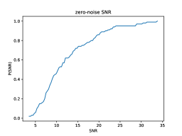
Figure 1: Cumulative SNR distribution for a synthetic population of 100 events drawn from the fiducial BBH population described in Section II.3. To avoid ambiguity, this figure shows the expected SNR (i.e., the SNR evaluated using a zero-noise realization).

One way to assess the performance of parameter inference is a probability-probability plots (usually denoted PP plot) Cook et al. (2012). Using RIFT on each source $k$, with true parameters $\mathbf{\lambda}_{k}$, we estimate the fraction of the posterior distributions which is below the true source value $\lambda_{k,\alpha}$ [$\hat{P}_{k,\alpha}(<\lambda_{k,\alpha})$] for each intrinsic parameter $\alpha$, again assuming all sources have zero spin. After reindexing the sources so $\hat{P}_{k,\alpha}(\lambda_{k,\alpha})$ increases with $k$ for some fixed $\alpha$, the top panel of Figure 3 shows a plot of $k/N$ versus $\hat{P}_{k}(\lambda_{k,\alpha})$ for all binary parameters. For the top panel, both injections and inference are performed with the same model, and the recovered probability distribution is consistent with $P(<p)=p$, as expected.

II.4 Zero noise runs to assess systematic biases

Our synthetic data consists of expected detector responses $h(t)$ superimposed on detector noise realization $n(t)$. The recovered posterior distribution’s properties and in particular maximum-likelihood parameters depend on the specific noise realization used. To disentangle the deterministic effects of waveform systematics from the stochastic impact of different noise realizations, we also repeat our analyses with the ”zero noise” realization: $n(t)=0$.

II.5 Model-model mismatch

Several previous investigations (e.g., Lindblom et al. (2008); Read et al. (2009); Lindblom et al. (2010); Cho et al. (2013); Hannam et al. (2010); Kumar et al. (2016); Pürrer and Haster (2020) and references therein) have phenomenologically argued that the magnitude of systematic biases are related to the model-model mismatch, a simple inner-product-based estimate of waveform similarity between two model predictions $h_{1}(\lambda)$ and $h_{2}(\lambda)$ at identical model parameters $\lambda$:

$${\cal M}(\lambda)=1-\max_{t_{c},\phi_{c}}\frac{|\left\langle h_{1}|e^{i(2\pi ft_{c}+\phi_{c})}h_{2}\right\rangle|}{|h_{1}||h_{2}|}$$ (3)

In this expression, the inner product $\langle a|b\rangle_{k}\equiv\int_{-\infty}^{\infty}2df\tilde{a}(f)^{*}\tilde{b}(f)/S_{h,k}(|f|)$ is implied by the k^th detector’s noise power spectrum $S_{h,k}(f)$, which for the purposes of waveform similarity is assumed to be the advanced LIGO instrument, H1. In practice we adopt a low-frequency cutoff $f_{\rm min}$ so all inner products are modified to

$$\langle a|b\rangle_{k}\equiv 2\int_{|f|>f_{\rm min}}df\frac{[\tilde{a}(f)]^{*}\tilde{b}(f)}{S_{h,k}(|f|)}.$$ (4)

Figure 2 shows the distribution of mismatches for our synthetic population, where $h_{1}$ is generated using SEOBNRv4 and $h_{2}$ with IMRPhenomD. For simplicity, we regenerate all signals at zero inclination, to avoid polarization-related effects associated with the precise emission direction. For our fiducial compact binary population, the mismatches between these two models are typically below $10^{-2}$, consistent with previous reports on systematic differences between these two waveforms and with their similarity to even more accurate models and simulations Bohé et al. (2017); Khan et al. (2016b); Pürrer and Haster (2020)

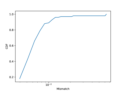
Figure 2: Cumulative Mismatch Distribution for population: For all the synthetic sources in our population, we evaluate the GW strain along the $z$ axis using SEOBNRv4 and IMRPhenomD, then compute the mismatch between them. This figure shows the cumulative distribution of these mismatches, most of which are slightly less than $10^{-2}$.

II.6 Marginalizing over waveform systematics

Suppose we have two models $A$ and $B$ for GW strain, and use them to interpret a particular GW source. We have prior probabilities $p(A|\lambda)$ and $p(B|\lambda)$, characterizing our relative confidence in these two models for a source with parameters $\lambda$. Suppose we have produced a RIFT analysis with each model for this event, and have marginal likelihood functions ${\cal L}_{A}(\lambda)$ and ${\cal L}_{B}(\lambda)$ evaluated at a single point $\lambda$. We can therefore construct the marginal likelihood for $\lambda$ by averaging over both models:

$${\cal L}_{av}(\lambda)=p(A|\lambda){\cal L}_{A}(\lambda)+p(B|\lambda){\cal L}_{B}(\lambda)$$ (5)

For simplicity the calculations in this work always adopt $p(A|\lambda)=p(B|\lambda)=1/2$. We can therefore transparently integrate multi-model inference into RIFT as follows. We assume we have a single grid of points $\lambda_{k}$ such that both $(\lambda_{k},{\cal L}_{A}(\lambda_{k})$ and $(\lambda_{k},{\cal L}_{B}(\lambda_{k})$ can be interpolated to produce reliable likelihoods and thus posterior distributions $p_{A}(\lambda)$ and $p_{B}(\lambda)$, respectively. At each point $\lambda_{k}$ we therefore construct ${\cal L}_{av}(\lambda_{k})$ by the above procedure. We then interpolate to approximate $\hat{\cal L}(\lambda)$ versus the continuous parameters $\lambda$.

Operationally speaking, we construct model-averaged marginal likelihoods by the following procedure. First, we construct a fiducial grid for models A and B, for example by joining the grids used to independently analyze A and B. We use ILE to evaluate ${\cal L}_{A}(\lambda_{k})$ and ${\cal L}_{B}(\lambda_{k})$ on this grid. We construct ${\cal L}_{av}(\lambda_{k})$ as above. We use the combinations $(\lambda_{k},{\cal L}_{av})$ with CIP, to construct a model-averaged posterior distribution.

Our procedure bears considerable resemblance to the approach suggested by Ashton and Khan, but we have organized the calculation differently. In that approach, AK used the evidences $Z_{A}=\int{\cal L}_{A}p(\lambda)d\lambda$ and $Z_{B}$ for the two waveform models. While we can compute both quantities with very high accuracy, we prefer to directly average between waveform models at the same choice of intrinsic parameters (i.e., via Eq. (5)) , to insure that marginalization over waveform models is completely decoupled from the interpolation techniques used to construct $\hat{{\cal L}}$ from the sampled data.

III Results

Using our fiducial BBH population, we generated 100 synthetic signals using IMRPhenomD, and another 100 synthetic signals with SEOBNRv4. For each signal, we performed parameter inference with both IMRPhenomD and SEOBNRv4. These inferences allow us both to assess the impact of waveform systematics in our fiducial population, and mitigate them.

III.1 Demonstrating and quantifying waveform systematics

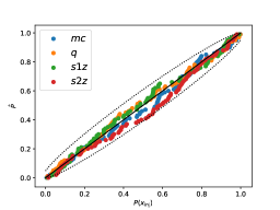
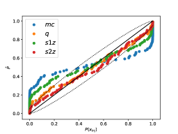
Figure 3: PP-plot of events injected with SEOBNRv4 and recovered with SEOBNRv4 (top panel) and IMRPhenomD (bottom panel) waveform. The dashed line indicates the 90% credible interval expected for a cumulative distribution drawn from 100 uniformly-distributed samples.

The PP plot provides the most compelling demonstration of waveform systematics’ pernicious impact. Ideally, when recovering a known model and a known population, we expect to recover the injected values as often as they occur, producing a diagonal PP plot. The top panel of Figure 3 shows precisely what we expect, when we inject and recover with the same model (here, SEOBNRv4). By contrast, the bottom panel shows a PP plot generated using inference from IMRPhenomD on the same SEOBNRv4 injections. The PP plot is considerably non-diagonal, reflecting frequent and substantial parameter biases in our fiducial population.

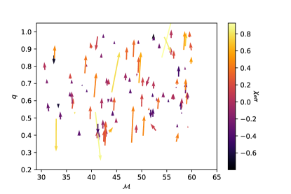
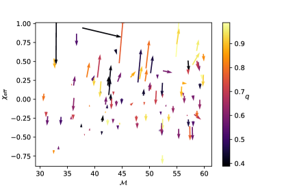
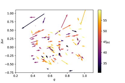
Figure 4: Vector plot showing amplitude-scaled offsets between SEOBNRv4 and IMRPhenomD for parameters $\mathcal{M}$ and $q$ (top panel), $\mathcal{M}$ and $\chi_{\rm eff}$ (middle panel) and $q$ and $\chi_{\rm eff}$ (bottom panel) as a function of the respective parameters with color map being the value of the parameter mentioned on the color scale.

Parameter biases introduced by waveform systematics vary in magnitude and direction over the parameter space. To illustrate these offsets for the parameters $x={\cal M},q,\chi_{\rm eff}$, we’ve evaluated the parameter shift $\Delta x$ between the mean inferred with IMRPhenomD and the mean inferred with SEOBNRv4, relative to $\sigma\rho$, which is a product of $\rho$ (the signal-to-noise ratio, a measure of the signal amplitude) and the statistical error (as measured by the standard deviation $\sigma$ of the posterior of the parameter $x$ in question). [The combination $\sigma\rho$ is approximately independent of signal amplitude, allowing us to measure the effect of waveform systematics for a fiducial amplitude.] Figure 4 shows a vector plot of these scaled offsets $\Delta x/\rho\sigma$, as a function of two of the parameters at a time. The length of the arrow corresponds to the scaled shifts in the parameters $\mathcal{M}$, $q$ and $\chi_{\rm eff}$, plotted against the injected parameter values. The color scale shows the remaining parameter. The top two panels show that shifts in $q=m_{2}/m_{1}$, $\chi_{\rm eff}=(m_{1}\chi_{1,z}+m_{2}\chi_{2,z})/(m_{1}+m_{2})$ are substantial. Parameter shifts for $q$ generally increase with $\chi_{\rm eff}$. Shifts in $\chi_{\rm eff}$ are generally positive for positive $\chi_{\rm eff}$, negative for negative $\chi_{\rm eff}$, and strongly dependent on mass ratio, with more substantial shifts at either comparable mass or at very high mass ratio, respectively. In both cases, chirp mass ${\cal M}$ has modest impact, with somewhat larger shifts occurring at somewhat larger values of chirp mass. Most extreme waveform systematics seem to be associated with large mass ratio.

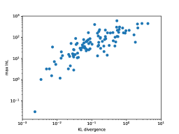
Figure 5: Figure showing KL-divergences between the two waveform models versus the log of the maximum likelihood for the combined posteriors of $\mathcal{M}$, $\it{q}$ and $\chi_{\rm eff}$.

Relative differences in mean value only imperfectly captures the differences between the two posteriors. As a sharper diagnostic that includes parameter correlations, we use the mean and covariance of each distribution in ${\cal M},q,\chi_{\rm eff}$ to generate a local gaussian approximation for each posterior, and then compute the KL divergence between these two gaussian approximations Lange et al. (2018). We expect more substantial differences and thus larger KL divergence for stronger signals, whose posteriors are more sharply constrained. To corroborate our intuition, Figure 5 shows a scatterplot, with these KL divergences on the horizontal axis and the largest value of $\ln{\cal L}$ on the vertical axis. As expected, for the strongest signals, differences between the two waveform models are the most pronounced.

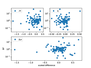
Figure 6: Figure showing Bayes factor (BF) for SEOBNRv4 versus IMRPhenomD plotted against differences between the SEOBNRv4 and IMRPhenomD waveforms for parameters $\mathcal{M}$, $\it{q}$ and $\chi_{\rm eff}$.

One might expect that large parameter offsets are more likely to occur when the data favors one model or another. While conceivably true asymptotically, for our specific synthetic population, we don’t find a strong correlation between the Bayes factor ($\mathcal{Z}_{\textsc{SEOBNRv4}}/\mathcal{Z}_{\textsc{IMRPhenomD}}$) and any parameter offsets. Figure 6 shows this Bayes factor (BF) plotted versus the scaled parameter offsets in ${\cal M},q,\chi_{\rm eff}$. Large offsets can occur without the data more strongly favoring one model or the other, and vice versa.

III.2 A PP plot test for marginalizing over waveform errors

We test our model-averaged waveform procedure using a full synthetic PP plot procedure. Specifically, we use the $n_{s}=100$ synthetic source parameters. For each source, we pick one waveform model $A,B$ with probabilities $p(A),p(B)$, and use it to generate the signal. We then analyze the signal using the model-averaged procedure described above.

As a concrete example, the top panel of Figure 7 shows our analysis of one fiducial event in our synthetic sample. The colored points show likelihood evaluations, with color scale corresponding to the marginalized likelihood evaluated with IMRPhenomD. The blue and black contours show the 90% credible intervals for SEOBNRv4 and IMRPhenomD, respectively; the two posteriors differ substantially, illustrating the impact of model systematics on parameter inference. The green contour shows our model-marginalized posterior. For comparison, the cross shows the injected source parameters, and the model was IMRPhenomD.

The bottom panel of Figure 7 shows one PP plot corresponding to applying our model-marginalized procedure to a population where each source is randomly selected from either IMRPhenomD or SEOBNRv4. The dotted line shows a 90% frequentist interval for the largest of four random cumulative distributions. This figure shows our PP plots are consistent with the diagonal, as desired.

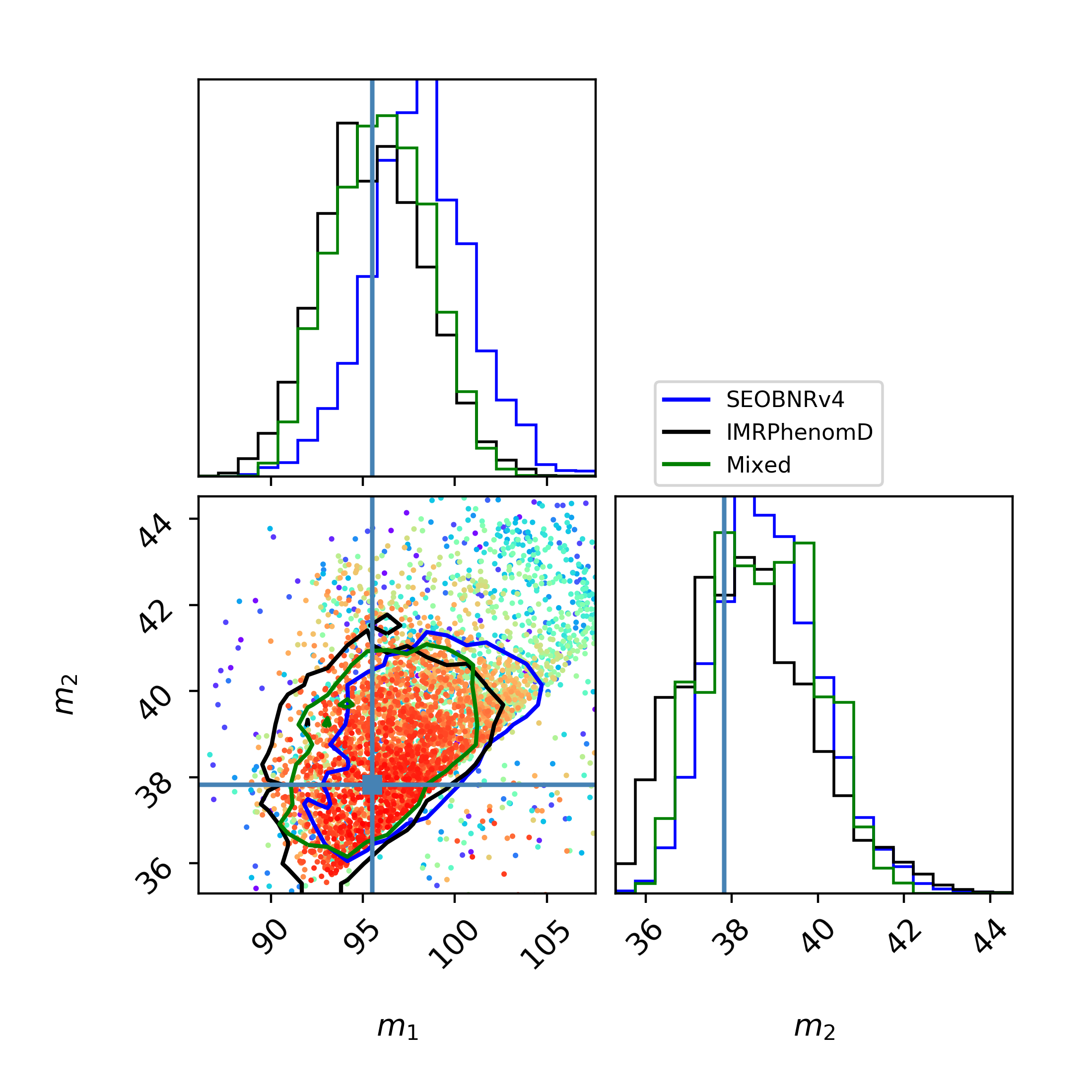
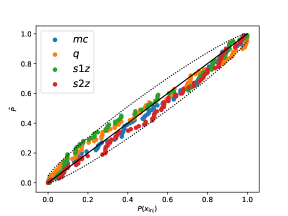
Figure 7: Top panel: example of a model averaged result. The blue and black curves show the 1D marginal distributions and 2D 90% credibles for SEOBNRv4 and IMRPhenomD inferences, respectively. The green curves show the corresponding model-averaged result. Bottom panel: PP plot test for our model-marginalized procedure.

IV Discussion

In this work, we performed simple tests which reproduce significant differences between the models SEOBNRv4 and IMRPhenomD, and can be extended to other available waveforms easily using RIFT, an efficient parameter estimation engine. The probability-probability (PP) plot test, a commonly used statistical test, can be used to confirm differences between waveform models and as shown in Fig. 3, parameter estimation performed using a model different from the injected model, gives a non-diagonal pp-plot for most parameters. We calculated the magnitude and direction of the offsets introduced due to using a waveform model different to the injected model, and these differences are higher for extreme case scenarios, as expected. A linear correlation between the KL divergence computed for the two models and the log of the maximum likelihood of the injected model, shows that high-SNR signal will have larger differences in the inferred parameter from various models. Because the most informative signals exhibit the largest parameter biases, waveform systematics have the potential to strongly contaminate population inference. Most importantly, we also demonstrated a method to mitigate these waveform systematics by marginalizing over the models used for parameter estimation analyses.

Our method requires as input some prior probabilities $p(X_{k}|\lambda)$ for different waveform models $X_{k}$. One way these prior probabilities could be selected is by waveform faithfulness studies between models and numerical relativity simulations. These fidelity studies inevitably suggest waveform models vary in reliability over their parameter space (e.g. Kumar et al. (2014, 2015)), suggesting $p(X_{k}|\lambda)$ will depend nontrivially on $\lambda$. Operationally, these model priors propagate into each model’s posterior inferences as if parameter inferences for model $X$ are performed using a model-dependent prior $\propto p_{\rm prior}(\lambda)p(X_{k}|\lambda)$, instead of a common prior for all models. RIFT can seamlessly perform these calculations at minimal added computational expense, while simultaneously returning results for each model derived from the conventional prior alone.

V Conclusions

Many waveform models exist currently that describe compact binary coalescences. Even though these are derived by solving Einstein’s equations, the various analytical or numerical approximation considered bring in differences and affect the parameter estimation process leading to biased interpretation of results. Averaging over the waveform models can mitigate these biases. Building on prior directly comparable work Ashton and Khan (2020), we have demonstrated an efficient method to perform such model marginalization.

Other techniques have been proposed to marginalize over waveform model systematics. Notably, several groups have proposed using the error estimates provided by their model regressions (e.g., the gaussian process error) Chua et al. (2020). Relative to regression-based methods, our method has two notable advantages. Our method can be immediately generalized to include multiple waveform models. Critically, we plan to introduce parameter-dependent weighting of the likelihood from a waveform, since different waveforms are accurate in different regimes. No other model-marginalization technique can presently provide this level of control.