Simulating the Cosmic Neutrino Background using Collisionless Hydrodynamics

Abstract

The cosmic neutrino background is an important component of the Universe that is difficult to include in cosmological simulations due to the extremely large velocity dispersion of neutrino particles. We develop a new approach to simulate cosmic neutrinos that decomposes the Fermi-Dirac phase space into shells of constant speed and then evolves those shells using hydrodynamic equations. These collisionless hydrodynamic equations are chosen to match linear theory, free particle evolution and allow for superposition. We implement this method into the information-optimized cosmological $N$-body code CUBE and demonstrate that neutrino perturbations can be accurately resolved to at least $k\sim 1$ $h\$Mpc^-1. This technique allows for neutrino memory requirements to be decreased by up to $\sim 10^{3}$ compared to traditional $N$-body methods.

1 Introduction

The cosmic neutrino background (C$\nu$B) has been robustly detected by observations of the cosmic microwave background perturbations (CMB) (Planck Collaboration et al., 2018). At $z\sim 1100$ when the primary CMB perturbations are set the neutrinos are highly relativistic; however, observations of neutrino oscillations (de Salas et al., 2018) suggest that at least one species of neutrino has mass $m_{\nu}\gtrsim 0.05$ eV and so should be non-relativistic today. Measuring the properties of the non-relativistic C$\nu$B has become one of the chief goals of upcoming cosmological experiments. Of principle importance is a measurement of the total neutrino mass $M_{\nu}=\sum m_{\nu}$ which, in conjunction with oscillation experiments, may also resolve the neutrino hierarchy and whether any neutrinos are massless. Currently cosmological constraints (e.g. Planck Collaboration et al. (2018); Palanque-Delabrouille et al. (2019)) of $M_{\nu}$ are significantly better than terrestrial ones (Aker et al., 2019).

The C$\nu$B is distinct in that it becomes massive but still remains quite hot and so does not cluster nearly as much on small scales as the dominant cold dark matter (CDM). The principle effect of this lack of clustering is a modulation of the matter power spectrum in a way that is sensitive to the neutrino energy density $\Omega_{\nu}$. If standard cosmology holds, where neutrinos are the only hot species and have the standard decoupling temperature $T_{\nu}=(4/11)^{1/3}T_{\rm CMB}$, then $\Omega_{\nu}h^{2}=M_{\nu}/93.14$ (Mangano et al., 2005). This technique for determining $M_{\nu}$ is a substantial challenge both because the modulation is small and because we principally measure not the underlying matter field but rather biased tracers of it such as galaxies. If $M_{\nu}$ is minimal, forecasts for DESI, EUCLID and CMB-S4 suggest that near future detections of the C$\nu$B using the matter power spectrum will be at most around $3\sigma$ (Brinckmann et al., 2019). Finding other observables sensitive to neutrinos is therefore critical to improve the robustness of the non-relativistic C$\nu$B detection. Alternatives that have been suggested include void statistics (Massara et al., 2015; Banerjee and Dalal, 2016a; Kreisch et al., 2019), the relative velocity effect (Zhu et al., 2014, 2016; Inman et al., 2015, 2017; Zhu and Castorina, 2019), scale-dependent halo bias (LoVerde, 2014; Chiang et al., 2018, 2019; Banerjee et al., 2019), differential neutrino condensation (Yu et al., 2017), and via galaxy spins (Yu et al., 2019).

It is therefore critical to accurately model the effects of neutrinos on large scale structure. The C$\nu$B has been included in simulations in a number of ways. The most straightforward methods invoke linear theory, either interpolating between precomputed results (Brandbyge and Hannestad, 2009) or integrating alongside the simulation (Ali-Haïmoud and Bird, 2013). These methods are quite fast and lead to the correct modulation of the matter power spectrum, but do not accurately resolve neutrino dynamics. The standard method to obtain correct neutrino behaviour is to use N-body particles which have large thermal velocities drawn from the Fermi-Dirac distribution, e.g. Brandbyge et al. (2008); Viel et al. (2010); Zennaro et al. (2017). The chief downside of this style of simulation is that the random velocities are so large that they introduce significant randomness into the neutrino density field that substantially erases the true perturbations on small scales. The effects of this Poisson noise can be suppressed through the use of many particles (Emberson et al., 2017) or through the use of hybrid methods where part of the evolution is linear (Brandbyge and Hannestad, 2010; Inman et al., 2015; Bird et al., 2018).

There are two methods employed in the literature that are Poisson noise free. The first is to use neutrino particles, but introduce regularity in the thermal velocities such that random clustering does not occur (Banerjee et al., 2018). In practice, this involves utilizing many particles per grid cell, with each cell having the same sampling of random velocities. The second is to instead solve the Boltzmann moment equations on a grid, which has no Poisson noise by construction. The difficulty here is that the Boltzmann moment equations are an infinite hierarchy of equations with no known truncation scheme consistent with the neutrino distribution. One approach is to close the hierarchy by utilizing linear theory for the stress terms in the momentum equation (Dakin et al., 2017) which works well provided that the pressure is always correlated with the density field. The other method is to use N-body particles for closure by using them to estimate the stress terms (instead of the density) (Banerjee and Dalal, 2016a).

In this paper we also solve the Boltzmann moment equations; however we do so by using a closure scheme that does not rely on either external transfer functions or N-body particles. We do this by decomposing the neutrino phase space into shells of uniform speed, for which a straightforward linear closure scheme exists. It is conceptually quite similar to the multiflow description of Dupuy and Bernardeau (2014, 2015), although we consider particles with the same speed rather than the same velocity. We show slices comparing our method and standard N-body in Fig. 1. The lack of Poisson noise is immediately evident. In Section 2 we motivate the closure scheme for the velocity shells. In Section 3 we discuss our numerical implementation of the method into the CUBE code (Yu et al., 2018). We then show results of these simulations, including comparisons to standard N-body methods, in Section 4. We discuss future optimizations and extensions in Sections 5 and 6.

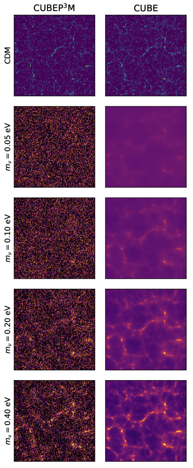
Figure 1: Slices of CDM (top row) and C$\nu$B (bottom four rows) density fields computed using CUBEP³M (left) and CUBE (right). The slices are 350 $h^{-1}$Mpc in width and 0.7 $h^{-1}$Mpc in depth. The hydrodynamic method used in CUBE is free from Poisson noise.

2 Theory

2.1 Vlasov Equation and Boltzmann Moment Equations

The phase space, $f(t,x^{i},v^{i})$, of collisionless particles is described by the Vlasov equation:

$$\frac{\partial f}{\partial t}+v^{i}\frac{\partial f}{\partial x^{i}}+g^{i}\frac{\partial f}{\partial v^{i}}=0,$$ (1)

also known as the collisionless Boltzmann equation. In an expanding Universe with scalefactor $a$, $t$ is the Newtonian time ($a^{2}dt=dt_{p}$), $x^{i}$ is the comoving coordinate ($adx^{i}=dx^{i}_{p}$), $v^{i}$ is the conjugate velocity ($v^{i}=dx^{i}/dt$) and $g^{i}$ is the gravitational acceleration field ($g^{i}=-a^{2}\partial\phi/\partial x^{i}$ where $\phi$ is the Newtonian potential) (Bertschinger, 1995; Inman and Pen, 2017). The initial conditions for the C$\nu$B is the relativistic Fermi-Dirac distribution:

$$\bar{f}_{\nu}=\frac{\beta^{3}}{6\pi\zeta(3)}\frac{1}{\exp[\beta v]+1}$$ (2)

where $\beta=m_{\nu}/T_{\nu}$ and the normalization is chosen such that the mean density is unity: $\bar{\rho}=\int d^{3}v\bar{f}(v)=1$.

Eq. 1 can be converted into a hierarchy of moment equations. We denote coarse-grained fields with the notation $\langle A(t,x^{i},v^{i})\rangle=\int d^{3}vAf$. We will concern ourselves with the the density, $\rho=\langle 1\rangle$, the momentum $\rho V^{i}=\langle v^{i}\rangle$, the stress-energy tensor $\rho\Sigma^{ij}=\langle v^{i}v^{j}\rangle$ and the third order heat tensor $\rho Q^{ijk}=\langle v^{i}v^{j}v^{k}\rangle$. The stress-energy tensor is often expanded as $\rho\Sigma^{ij}=\rho V^{i}V^{j}+\rho\sigma^{ij}$ where $V^{i}$ is the velocity field and $\sigma^{ij}=\rho^{-1}\langle(v^{i}-V^{i})(v^{j}-V^{j})\rangle$ is the velocity dispersion. $\rho Q^{ijk}$ can be expanded as $\rho Q^{ijk}=\rho V^{i}V^{j}V^{k}+\rho V^{i}\sigma^{jk}+\rho V^{j}\sigma^{ik}+\rho V^{k}\sigma^{ij}+\rho q^{ijk}$ where $\rho q^{ijk}=\langle(v^{i}-V^{i})(v^{j}-V^{j})(v^{k}-V^{k})\rangle$ is heat flux tensor with associated heat flux $(1/2)\rho q^{iik}$.

By integrating Eq. 1 over velocity we can obtain their equations of motion. These are the continuity equation:

$$\frac{\partial}{\partial t}\rho+\frac{\partial}{\partial x^{k}}\rho V^{k}=0,$$ (3)

the momentum equation:

$$\frac{\partial}{\partial t}\rho V^{i}+\frac{\partial}{\partial x^{k}}\rho\Sigma^{ik}=\rho g^{i}$$ (4)

and the stress-energy equation

$$\frac{\partial}{\partial t}\rho\Sigma^{ij}+\frac{\partial}{\partial x^{k}}\rho Q^{ijk}=\rho V^{i}g^{j}+\rho V^{j}g^{i}.$$ (5)

2.2 Hydrodynamic Equations

We wish to re-express these equations in terms of hydrodynamic variables. To that end, we expand the velocity dispersion in terms of primitive variables $\rho\sigma^{ij}=P\delta^{ij}+\pi^{ij}$ where $P$ is the pressure and $\pi^{ij}$ is the shear stress, which is traceless, $\pi^{ii}=0$, and symmetric, $\pi^{ij}=\pi^{ji}$. We now require equations of motion for $P$ and $\pi^{ij}$ which can be obtained from Eq. 5. Instead of using the stresses directly, it is convenient to use the energy, $E$, and anisotropic stress, $\tau^{ij}$. The energy is related to the trace of the stress-energy tensor

$$E =\frac{1}{2}\rho\Sigma^{ii}$$

$$=\frac{1}{2}\rho V^{2}+\frac{3}{2}P$$

$$=\frac{1}{2}\rho V^{2}+\frac{P}{\gamma-1}$$ (6)

which matches the definition of the energy of an ideal fluid with $\gamma=5/3$ (Mitchell et al., 2013). The anisotropic stress is then the traceless component:

$$\tau^{ij} =\rho\Sigma^{ij}-\frac{1}{3}\rho\Sigma^{kk}\delta^{ij}$$ (7)

$$=\rho V^{i}V^{j}-\frac{1}{3}\rho V^{2}\delta^{ij}+\pi^{ij}.$$

The equations of motion in terms of the conservative variables are then

$$\frac{\partial}{\partial t}\rho V^{i}+\frac{\partial}{\partial x^{k}}\left[\rho V^{i}V^{k}+P\delta^{ik}+\pi^{ik}\right]=\rho g^{i},$$ (8)

$$\frac{\partial}{\partial t}E+\frac{\partial}{\partial x^{k}}\left[EV^{k}+PV^{k}+V^{l}\pi^{lk}+\frac{1}{2}\rho q^{iik}\right]=\rho V^{k}g^{k}$$ (9)

and

$$\frac{\partial}{\partial t}\tau^{ij} +\frac{\partial}{\partial x^{k}}\left[\tau^{ij}V^{k}+PV^{i}\delta^{jk}+PV^{j}\delta^{ik}-\frac{2}{3}PV^{k}\delta^{ij}\right.$$

$$\left.+V^{i}\pi^{jk}+V^{j}\pi^{ik}-\frac{2}{3}V^{l}\pi^{lk}\delta^{ij}+\rho q^{ijk}-\frac{1}{3}\rho q^{llk}\delta^{ij}\right]$$

$$=\rho V^{i}g^{j}+\rho V^{j}g^{i}-\frac{2}{3}\rho V^{k}g^{k}\delta^{ij}$$ (10)

2.3 Closing the Hierarchy

Solving these equations is exceptionally challenging due to the non-trivial stresses and heat tensor which are present even in linear theory. Strategies that have been employed to estimate the higher moments include linear theory (Dakin et al., 2017), using N-body particles to estimate higher moments (Pueblas and Scoccimarro, 2009; Banerjee and Dalal, 2016b), or the “Zero Heat Flux” approximation which sets $\rho q^{ijk}=0$ (Vorobyov and Theis, 2006; Mitchell et al., 2013).

An alternate approach is to try to deduce a (potentially nonlinear) equation of state for the heat flux which depends only on the hydrodynamic variables (see, e.g., Hammett and Perkins (1990); Chust and Belmont (2006); Wang et al. (2015)). To do this we will consider two test problems: the free evolution of particles and the linearized evolution of phase space.

2.3.1 Free Evolution of Particles

We first consider the free evolution ($g^{i}=0$) of collisionless particles. In this case, the exact solution to Eq. 1 is given in Fourier space by:

$${\rm FT}[f]={\rm FT}[f(t_{i})]\exp[-ik^{j}v^{j}(t-t_{i})].$$ (11)

If we now consider an initial distribution consisting solely of particles with the same velocity: $f(t_{i})\propto\rho(t_{i},x^{i})/(4\pi v^{2})\delta_{D}(v-u)$ the density field is given by:

$${\rm FT}[\rho]={\rm FT}[\rho(t_{i},x^{i})]j_{0}(ku(t-t_{i})).$$ (12)

The inverse Fourier transform of $j_{0}(ku(t-t_{i}))$ is $\delta_{D}(r-u(t-t_{i}))/(4\pi r^{2})$ and so this can be thought of as the convolution of the initial density field with the inverse square law. In general, Eq. 12 satisfies the wave-like spherical Bessel equation in real space:

$$\frac{\partial^{2}}{\partial t^{2}}\rho+\frac{2}{t-t_{i}}\frac{\partial}{\partial t}\rho-u^{2}\frac{\partial^{2}}{\partial x^{i}\partial x^{i}}\rho=0.$$ (13)

The C$\nu$B is initially homogeneous, $\rho(t_{i},x^{i})=1$, and so no direct convolution needs to be performed.

2.3.2 Linearized Vlasov Equation

We next consider the Vlasov equation linearized about some initial homogeneous and isotropic velocity distribution $f(t_{i},x,v)=\bar{f}(v)$:

$$\frac{\partial f}{\partial t}+v^{i}\frac{\partial f}{\partial x^{i}}+g^{i}\frac{\partial\bar{f}}{\partial v^{i}}=0.$$ (14)

We first remark that “linearized” is a misnomer in our particular application: since neutrinos are a small component ($f_{\nu}\ll 1$) the Vlasov equation is already approximately linear as $g^{i}$ is approximately independent of neutrino density. Instead, we are replacing a derivative term with a source term. This is precisely why the “linear response” method does not produce accurate neutrino power spectra despite neutrinos remaining linear (e.g. $\delta_{\nu}\ll 1$) at all times. Nonetheless, we will use the standard terminology throughout. The linear response solution to this equation is given in Fourier space by (Gilbert, 1966; Ali-Haïmoud and Bird, 2013):

$${\rm FT}[f]=\int_{t_{i}}^{t}dt^{\prime}(-{\rm FT}[g^{i}])\frac{\partial\bar{f}}{\partial v^{i}}\exp[-ik^{j}v^{j}(t-t^{\prime})].$$ (15)

The moments are then given by:

$${\rm FT}[\rho] =\int_{0}^{\infty}dv4\pi v^{2}\bar{f}(v)\int_{t_{i}}^{t}dt^{\prime}(-ik^{j}{\rm FT}[g^{j}])(t-t^{\prime})j_{0}(kv(t-t^{\prime}))$$ (16)

$$ik^{i}{\rm FT}[\rho V^{i}] =\int_{0}^{\infty}dv4\pi v^{2}\bar{f}(v)\int_{t_{i}}^{t}dt^{\prime}(ik^{j}{\rm FT}[g^{j}]\cos[kv(t-t^{\prime})]$$ (17)

$$ik^{i}ik^{j}{\rm FT}[\rho\Sigma^{ij}] =\int_{0}^{\infty}dv4\pi v^{2}\bar{f}(v)v^{2}k^{2}\int_{t_{i}}^{t}dt^{\prime}(-ik^{j}{\rm FT}[g^{j}])(t-t^{\prime})j_{0}(kv(t-t^{\prime}))$$ (18)

$$ik^{i}ik^{j}ik^{k}{\rm FT}[\rho Q^{ijk}] =\int_{0}^{\infty}dv4\pi v^{2}\bar{f}(v)v^{2}k^{2}\int_{t_{i}}^{t}dt^{\prime}(ik^{j}{\rm FT}[g^{j}]\cos[kv(t-t^{\prime})]$$ (19)

where we have omitted the homogeneous terms. It is immediately clear that density fields can be composed as sums over velocity shells. That is, if the background distribution with $\bar{f}_{u}=1/(4\pi v^{2})\delta_{D}(v-u)$ has moments such as $\rho_{u}$, then a more general distribution function $\bar{f}$ has $\rho=\int_{0}^{\infty}du4\pi u^{2}\bar{f}\rho_{u}$ (Inman and Pen, 2017). Furthermore, these shells have simple higher moments. In particular, the stress-energy tensor can be written entirely as an isotropic pressure $\rho\Sigma^{ij}=\rho\sigma^{ij}=P\delta^{ij}=\rho u^{2}\delta^{ij}$ and so the density satisfies the wave equation:

$$\frac{\partial^{2}}{\partial t^{2}}\rho-u^{2}\frac{\partial^{2}}{\partial x^{i}\partial x^{i}}\rho=-\frac{\partial}{\partial x^{i}}g^{i}.$$ (20)

Substituting this relationship and the linearized Eq. 3 into the linearized Eq. 5 leads to:

$$\frac{\partial}{\partial x^{k}}Q^{ijk} =\frac{\partial}{\partial x^{k}}(u^{2}V^{k}\delta^{ij})$$

$$=\frac{\partial}{\partial x^{k}}\left[u^{2}(V^{i}\delta^{jk}+V^{j}\delta^{ik}+V^{k}\delta^{ij})+q^{ijk}\right]$$ (21)

or

$$\frac{\partial}{\partial x^{k}}q^{ijk} =\frac{\partial}{\partial x^{k}}\left[-u^{2}V^{i}\delta^{jk}-u^{2}V^{j}\delta^{ik}\right]$$

$$=-u^{2}\frac{\partial V^{i}}{\partial x^{j}}-u^{2}\frac{\partial V^{j}}{\partial x^{i}}.$$ (22)

Linear velocity fields are curl free and can be written in terms of a velocity potential $V^{i}=\partial\phi_{v}/\partial x^{i}$ which leads to

$$\frac{\partial}{\partial x^{k}}q^{ijk} =-2u^{2}\frac{\partial^{2}\phi_{v}}{\partial x^{i}\partial x^{j}}.$$ (23)

The symmetric form of $q^{ijk}$ satisfying this is then given by:

$$q^{ijk} =-2u^{2}\frac{\partial}{\partial x^{i}}\frac{\partial}{\partial x^{j}}\frac{\partial}{\partial x^{k}}\nabla^{-2}\phi_{v}$$ (24)

$$=-\frac{2}{3}u^{2}\nabla^{-2}\left[\frac{\partial}{\partial x^{i}}\frac{\partial}{\partial x^{j}}V^{k}+\frac{\partial}{\partial x^{i}}\frac{\partial}{\partial x^{k}}V^{j}+\frac{\partial}{\partial x^{j}}\frac{\partial}{\partial x^{k}}V^{i}\right]$$ (25)

where $\nabla^{-2}$ denotes the inverse Laplacian.

2.3.3 Shell Equations of Motion

Unfortunately, it is unclear how to best generalize the linear heat flux of a shell once nonlinear evolution occurs. Simply using Eq. 2.3.2 for the heat tensor leads to an energy flux of $(P-\bar{\rho}u^{2})V^{k}+\pi^{ij}$ which could be $0$, the nonlinear fluctuation of $P$ or something else entirely. Lacking a nonlinear scheme, we instead opt for a particularly simple closure choice that allows for the shell equations to be independent of $u$:

$$\frac{\partial}{\partial x^{k}}\rho q^{ijk}=\frac{\partial}{\partial x^{k}}\left(-\rho\sigma^{ik}V^{j}-\rho\sigma^{jk}V^{i}\right)$$ (26)

which yields the much simplified continuity equations for stress-energy:

$$\frac{\partial}{\partial t}E+\frac{\partial}{\partial x^{k}}EV^{k} =\rho V^{k}g^{k}$$ (27)

$$\frac{\partial}{\partial t}\tau^{ij}+\frac{\partial}{\partial x^{k}}\tau^{ij}V^{k} =\rho V^{i}g^{j}+\rho V^{j}g^{i}-\frac{2}{3}\rho V^{k}g^{k}\delta^{ij}.$$ (28)

The complete set of equations for a shell is therefore: Eqs. 3, 8, 27 and 28. In the absence of gravity, these equations collapse down to wave dynamics. We note that the wave equation allows for superposition which resembles shell crossing. In this work we make one further simplification and neglect the shear stress entirely, $\pi^{ij}=0$, leading to ideal collisionless hydrodynamics. This simplification is still consistent with linear theory but allows us to save substantial resources by not solving Eq. 28. We consider two alternative schemes, the isothermal and ideal gas approximations, in the Appendix.

Let us lastly comment on the difference between this approach and linear response. In linear response approximations are made to the gravitational terms, i.e. $\rho g^{i}\rightarrow\bar{\rho}g^{i}$. In Eqs. 27 and 28 we have made approximations to the hydrodynamic fluxes, but kept gravitational terms fully intact. We therefore expect this approach to work significantly better as it retains linearity in the neutrino perturbations themselves.

3 Methods

In this section we describe our implementation of the neutrino solver into the CUBE code (Yu et al., 2018). CUBE is a refactored version of CUBEP³M (Harnois-Déraps et al., 2013) designed to use the minimum amount of memory possible: 6 bytes per particle. It features a three level force decomposition: a “coarse” particle mesh force over $n_{c}$ cells where the only global FFT is performed, a “fine” particle mesh force with resolution $n_{f}=4n_{c}$ where local FFTs are performed, and a direct particle-particle (PP) force at the cell level. CUBE is parallelized with both OpenMP and co-array Fortran. Both CUBE and CUBEP³M are publicly available.

3.1 Single-Shell Hydrodynamics

In principle, any method to solve the hydrodynamical equations can be used for collisionless hydrodynamics. For our purposes, we have opted for a simple dimensionally split Eulerian grid method. Overall, the code is very similar to the example code of Trac and Pen (2003), except with the relaxing algorithm replaced by an HLL approximate Riemann solver (Harten et al., 1983). While we don’t expect neutrinos to require particularly high spatial resolution, we allow for it by using a piecewise linear flux calculation with a nonlinear flux limiter. The gravitational force is considered as a source term, and coupled to the N-body code in the same way as the magnetohydrodynamics code was coupled to CUBEP³M. This means that density is conserved to machine precision, but momentum and energy are not. Since the hydrodynamic grid need not have the same number of cells as the gravitational grid, we simply interpolate the values of all gravitational forces computed within a hydrodynamical cell. If the grid is coarser than $n_{f}/2$ or $n_{c}/2$ this introduces force artifacts on the fine/coarse grid scale since only one cell is ever buffered. Since this is, by construction, subgrid for the neutrinos, and indeed the neutrino perturbations are themselves highly suppressed anyways, we have not encountered any issues.

3.2 Cosmic Neutrino Background

Utilizing this technique for the the C$\nu$B requires the simulation of multiple velocity shells, each with density $\rho_{u}$, which can then be integrated over to obtain the neutrino density: $\rho_{\nu}=\int_{0}^{\infty}du4\pi u^{2}\bar{f}_{\nu}\rho_{u}$. The shell densities can be computed using the methods of Subsection 3.1. Optimally performing this integration was studied by Lesgourgues and Tram (2011) who found that Gauss-Laguerre integration is the best choice. We therefore use this quadrature strategy and find that only three integration points provide accurate results. The proper shell velocities are then $\{418,2310,6320\}\times(1+z)(0.05{\rm eV}/m_{\nu})$ km s^-1 with the fastest shell becoming non-relativistic at $z\sim 50(m_{\nu}/0.05{\rm eV})$ km s^-1.

Since CDM perturbations are typically set at $z\sim 100$ and we do not want to be evolving neutrinos until they are safely non-relativistic, we employ the “late start” approach developed in Inman et al. (2015). Specifically, CDM perturbations are generated at some intermediate redshift $z_{\nu}$ and then propagated backwards to the initial redshift $z_{i}$ with a growth factor that assumes neutrinos are homogeneous: $D_{+}\sim(a_{i}/a_{\nu})^{1-3f_{\nu}/5}$ (Bond et al., 1980). The forward evolution proceeds in two phases: between $z_{i}$ and $z_{\nu}$ the CDM evolves alone (i.e. $\delta_{\nu}=0$). This precisely undoes the modified growth factor on linear scales whereas on nonlinear scales the neutrino perturbations are negligible anyways. After $z_{\nu}$ both the CDM and the C$\nu$B are simultaneously evolved.

Since the shell velocities are quite large, the neutrino timestep is required to be quite small. We allow each velocity shell to have its own grid size which allows faster shells to be coarser and hence have shorter timesteps. A future optimization is to allow neutrinos to take multiple timesteps between each CDM one. It may also be possible to allow shells to start at different redshifts, e.g., when their perturbations become dynamically relevant for the simulation.

3.3 Initial Conditions

Since we do not have transfer functions for individual momenta (although in principle these can be extracted from Boltzmann codes), we opt for approximate initial conditions for each velocity shell. To determine an approximate solution for each shell, we first consider their linear equations of motion, Eq. 20 (this can also be seen by differentiating Eq. 16 twice):

$$\frac{\partial^{2}\delta_{u}}{\partial t^{2}}+k^{2}u^{2}\delta_{u}=a^{2}(-k^{2}\phi).$$ (29)

On large scales, where $k$ is small, the second term is negligible and $\delta_{u}\simeq\delta_{c}$. On small scales, the fluid responds instantaneously and the solution is $\delta_{u}\simeq(k/k_{u})^{2}\delta_{c}$ where $k_{u}=\sqrt{(3/2)\Omega_{m}a}H_{0}/u$ is the free streaming scale of the shell (Inman and Pen, 2017). We utilize the following approximation:

$$\rho_{u}=1+\delta_{u}=1+\delta_{c}\frac{1}{1+\lambda k/k_{u}+(k/k_{u})^{2}}.$$ (30)

The corresponding velocity field is obtained via the continuity equation:

$$V^{i}_{u}=V^{i}_{c}\frac{1+1.5\lambda k/k_{u}+2(k/k_{u})^{2}}{(1+\lambda k/k_{u}+(k/k_{u})^{2})^{2}}.$$ (31)

In the simulations used in this paper we used $\lambda=1.$ which is appropriate for $z_{\nu}=0$; however, we have subsequently solved for the optimal value of $\lambda$ and find that $\lambda=0.75,0.76,0.77,$ and $0.82$ for $m_{\nu}=0.05,0.10,0.20$ and $0.40$ at $z_{\nu}=10$. These values are are rather unchanged at $z_{\nu}=5$ but increase towards $1$ at $z_{\nu}=0$. Utilizing a constant $\lambda=0.75$ at either $z_{\nu}=10$ or $5$ produces neutrino density and velocity transfer functions accurate to around 10% regardless of neutrino mass.

When computing the initial momentum density we opt to include the second order term, i.e. $\rho V^{k}=(1+\delta_{u})V_{u}^{k}$ rather than just $V_{u}^{k}$. Likewise, the initial energy is therefore

$$E_{u}=\rho_{u}\left[\frac{1}{2}V_{u}^{2}+\frac{u^{2}}{\gamma-1}\right]$$ (32)

with the kinetic term included.

4 Results

We run simulations of neutrinos of masses 0.05 eV, 0.10 eV, 0.20 eV and 0.40 eV using both CUBE and CUBEP³M. We keep the initial Gaussian noise realization equivalent between the two simulations and use the same number of particles, but otherwise allow them to run independently. Because the neutrinos are not coupled to the particle-particle force, we run CUBE without the direct force. Importantly, this means that the CUBEP³M simulations have better force resolution as they include the pairwise force on small scales. For cosmological parameters, we match those of Cataneo et al. (2019) so that we can compare to the high resolution results computed in that work. Specifically, we use a flat universe with fixed $1-\Omega_{\Lambda}=\Omega_{m}=\Omega_{c}+\Omega_{b}+\Omega_{\nu}=0.291$, $\Omega_{b}=0.047$, $h=0.6898$, and implicitly varying $\Omega_{c}$ via $\Omega_{\nu}=m_{\nu}/93.14/h^{2}$. For initial conditions we use $A_{s}=2.442\times 10^{-9}$ and $n_{s}=0.969$. In all cases we use $256^{3}$ CDM particles and simulate only a single massive neutrino species. In CUBEP³M the C$\nu$B is resolved by $256^{3}$ N-body particles, whereas in CUBE they are resolved by three fluids with grid resolution of $256^{3}$. The only exception is for the $m_{\nu}=0.05$ eV case where we used $128^{3}$ grid cells for the fastest shell. In this simulation we also decreased the CFL condition from 0.7 to 0.5 as we noticed some slight oscillations on small scales in the output. In all simulations for both codes we use $z_{i}=100$ and $z_{\nu}=10$. We show slices of CDM and C$\nu$B density fields in Fig. 1 which demonstrate well the lack of Poisson noise in the hydrodynamic simulations.

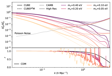
Figure 2: (Top) Ratio of C$\nu$B power spectra to the CDM one from hydrodynamics (solid), N-body (dashed) and linear theory (dotted). Also shown are the theoretical Poisson noise (dotted grey) and results from high resolution N-body simulations from Cataneo et al. (2019) (solid bands). (Bottom) The correlation coefficient between CUBE and CUBEP³M. The black band is the coefficient between CDM in the neutrinoless simulations.

We show the ratio of the C$\nu$B power spectra to the CDM one in the top panel of Fig. 2. Solid lines utilize the collisionless hydrodynamics approach, dashed lines the particles, dotted lines are linear theory results computed using CAMB (Lewis et al., 2000), and bands are the high-resolution simulations from Cataneo et al. (2019). For the lighter neutrino species the hydrodynamic simulations provide significantly better resolution due to lack of Poisson noise, whereas for the heavier ones it is merely comparable (although a lack of power seems preferable to an artificial enhancement). In the bottom panel we show the correlation coefficient between the two codes, defined as the ratio of the crosspower spectrum to the square root of the geometric mean of the autopower spectra. In general, this would go to zero when Poisson noise kicks in. To cancel shot noise in the power spectrum, we divide the neutrino particles randomly into two groups and compute the cross power as described in Inman et al. (2015). For $m_{\nu}<0.2$ eV this is very noisy due to the low particle number. However, for the heavier neutrino species it does do quite well and we find the hydrodynamics approach is well correlated to at least $k\sim 1$ $h^{-1}$Mpc.

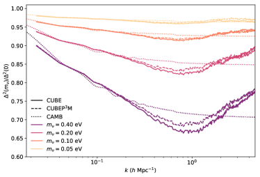
Figure 3: The suppression of the matter power spectrum as a function of neutrino mass. Dotted lines are linear theory from CAMB, dashed are computed using CUBEP³M, and solid are from CUBE.

The modulation of the matter power spectrum is shown in Fig. 3. CUBE yields the same result as CUBEP³M, matching linear theory on large scales but with an enhanced dip on nonlinear ones. On nonlinear scales CUBE and CUBEP³M very slightly disagree. We suspect that this is due to the difference in force calculation between the codes which results in slightly different power spectra.

5 Discussion

In an ideal simulation method neutrinos would increase memory and computation time by $\mathcal{O}(f_{\nu})$. Our method can satisfy the first criterion easily. As an example, we consider the hypothetical requirements to run a TianNu scale simulation (Emberson et al., 2017) with the CUBE code. TianNu evolved nearly three trillion particles, mostly neutrinos, in a cubic volume of width 1200 $h^{-1}$Mpc. Due to Poisson noise, TianNu only resolved neutrino perturbations to $k\sim 1$ $h\$Mpc^-1 which generically requires a grid with $\sim 1024$ cells per dimension to resolve. With our new hydrodynamical method, this would require $3\times 5\times 1024^{3}$ floating point numbers. This may be compared to the number required in TianNu, $6\times 13824^{3}$ floating point numbers, a savings of approximately $\sim 10^{3}$. The memory usage could be further decreased if faster shells are allowed to be less resolved. CUBE also has a significant CDM memory compression scheme which allows CDM memory reduction to as low as 6 bytes per particle (from 28 in CUBEP³M). In total, the TianNu simulation could be run utilizing around 40 times less memory to store particles.

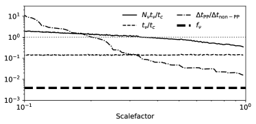
Figure 4: Relative time taken in neutrino and CDM computations from the $0.05$ eV simulation. The dashed line is the ratio of the physical time per timestep spent in the neutrino hydrodynamic subroutines to the CDM subroutines. The solid black line is the hypothetical ratio if individual timesteps are used for the neutrinos. The dash-dotted line is the ratio of the PP timestep to non-PP timesteps in a CDM only simulation.

In our current implementation the neutrino computations are quite fast compared to the CDM ones, however the total computation time is extended well beyond an $\mathcal{O}(f_{\nu})$ increase due to the short time step required by the neutrinos. Nonetheless, we are optimistic that this can be resolved by individual timestepping, where neutrinos take many more short timesteps than CDM. To obtain an idea of how much improvement can be obtained, we extract various timing quantities at each timestep: the time taken in the CDM subroutines ($t_{c}$ - note that this includes the force calculation, which has some neutrino operations as well), the time taken in the neutrino hydrodynamic routines ($t_{\nu}$), the required CDM timestep ($\Delta t_{c}$) and the required neutrino timestep ($\Delta t_{\nu}$) utilizing CFL=0.5. The number of neutrino steps that can be taken per CDM one is then given by $N_{\nu}=\Delta t_{c}/\Delta t_{\nu}$.

In Fig. 4 we show the ratio of the time necessary for neutrino calculations $N_{\nu}t_{\nu}$ compared to the time needed for CDM ones $t_{c}$ for the most challenging $0.05$ eV case. At high redshifts, the neutrino computations are substantial; however, at lower redshifts they quickly become subdominant. Bird et al. (2018) demonstrated that neutrinos with velocities $\gtrsim 100$ km s^-1 can be treated with linear response down to $z\sim 1$ and so we expect that we can always set $z_{\nu}$ such that neutrinos are subdominant. Indeed when the subgrid pairwise force, which requires a much smaller timestep as well, is also used the neutrinos may even become a negligible fraction. We ran a single CDM only simulation using CUBE with the PP force enabled with an extended range of one fine cell. The dash-dotted line in Fig. 4 shows the ratio of the timestep required for the PP force compared to other non-PP timesteps, giving an estimate of the scaling when subgrid forces are included. CUBE is currently undergoing optimizations for upcoming large scale simulations, and we hope to include individual timestepping in a subsequent update.

6 Conclusion

We have solved the Vlasov equation for the C$\nu$B using a novel technique based on decomposing the homogeneous phase space into velocity shells which are then evolved via a closed set of Boltzmann moment equations. We have found this approach to accurately model the neutrino perturbations well into the nonlinear regime. This method does not have Poisson noise, which plagues the more common particle based methods.

To model the C$\nu$B we have been interested in subsonic shells ($V\ll u$). A natural extension is to look for approximate closure schemes in the supersonic regime, which could be useful for warm or cold dark matter. When simulated with particles warm dark matter is known to exhibit artificial fragmentation (Wang and White, 2007) which may be ameliorated through the use of hydrodynamic equations. Of course, while the equations we employed are consistent with CDM linear evolution, and do allow for some level of shell crossing, it would be quite shocking if they provided a useful model of CDM. It is intriguing, however, to consider the closure relation for a known system, the Schrödinger equation, which approximates CDM above the de Broglie wavelength. For the coarse-grained Wigner approximation, the exact solution is given by $q^{ijk}=\hbar^{2}/(4m^{2})\nabla^{i}\nabla^{j}\nabla^{k}\phi_{v}$ (Uhlemann et al., 2014), which is very analogous to Eq. 24 with the “momentum” transformed to a quantum operator: $\sqrt{8}mu\rightarrow-i\hbar\nabla$. This is simply due to the fact that linear theory and the Schrödinger method both have velocity potentials, but nonetheless the similar form of the heat flux could provide a starting point for further investigations. It may also be more natural to treat potential dark matter interactions with hydrodynamic equations (e.g. Kummer et al. (2019)).

Appendix A Isothermal and Ideal Gas Approximations

In this section we test to what extent the isothermal and ideal gas approximations can be used to model the shells. For the isothermal gas, we assume that $P=\rho u^{2}$ at all times, with soundspeed $c_{s}=u$. We show the results in Fig. 5. In the top panel the solid coloured lines show the isothermal approximation, whereas the solid black lines show the collisionless hydrodynamics result. The bottom panel shows the difference in correlation coefficient between the isothermal gas and the collisionless hydrodynamics, i.e. negative values indicate collisionless hydrodynamics is better correlated. We find that the isothermal approximation appears to overpredict neutrino perturbations, but remains well correlated with the particle field.

Figure 5: (Top) Ratio of C$\nu$B power spectra, calculated using the isothermal gas approximation, to the CDM one. Black curves are the results from Fig. 2. (Bottom) Difference in correlation coefficient between iosthermal gas and N-body, and collisionless hydrodynamics and N-body.

For the ideal gas approximation, we employ the ideal gas energy equation:

$$\frac{\partial}{\partial t}E+\frac{\partial}{\partial x^{k}}\left[(E+P)V^{k}\right]=\rho V^{k}g^{k}.$$ (A1)

Because the flux $(E+P)V^{k}$ is simply proportional to $V^{k}$ upon linearization, the same as in collisionless hydrodynamics, we expect that we can reproduce linear evolution by simply changing the initial energy to:

$$E_{u}=\rho_{u}\left[\frac{1}{2}V_{u}^{2}+\frac{u^{2}}{\gamma(\gamma-1)}\right]$$ (A2)

and the sound speed is the standard $\sqrt{\gamma P/\rho}$. We show the result in Fig. 6 which shows that the ideal gas approximation slightly underpredicts neutrino perturbations. Again, this does not result in a substantially worsened correlation coefficient.

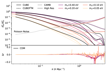
Figure 6: Same as Fig. 6 but using the ideal gas approximation.

We conclude that both approximations are sufficient to model the C$\nu$B, although perhaps slightly less accurate than collisionless hydrodynamics. As both isothermal and ideal gases are commonly included in cosmological codes it is therefore straightforward for these codes to include Poisson-noise free neutrino perturbations provided they can simulate multiple fluids simultaneously.

References

- Planck Collaboration et al. (2018) Planck Collaboration, N. Aghanim, Y. Akrami, M. Ashdown, J. Aumont, C. Baccigalupi, M. Ballardini, A. J. Banday, R. B. Barreiro, N. Bartolo, et al., arXiv e-prints arXiv:1807.06209 (2018), 1807.06209.
- de Salas et al. (2018) P. F. de Salas, D. V. Forero, C. A. Ternes, M. Tortola, and J. W. F. Valle, Phys. Lett. B782, 633 (2018), 1708.01186.
- Palanque-Delabrouille et al. (2019) N. Palanque-Delabrouille, C. Yèche, N. Schöneberg, J. Lesgourgues, M. Walther, S. Chabanier, and E. Armengaud, arXiv e-prints arXiv:1911.09073 (2019), 1911.09073.
- Aker et al. (2019) M. Aker, K. Altenmüller, M. Arenz, M. Babutzka, J. Barrett, S. Bauer, M. Beck, A. Beglarian, J. Behrens, T. Bergmann, et al., arXiv e-prints arXiv:1909.06048 (2019), 1909.06048.
- Mangano et al. (2005) G. Mangano, G. Miele, S. Pastor, T. Pinto, O. Pisanti, and P. D. Serpico, Nuclear Physics B 729, 221 (2005), hep-ph/0506164.
- Brinckmann et al. (2019) T. Brinckmann, D. C. Hooper, M. Archidiacono, J. Lesgourgues, and T. Sprenger, J. Cosmology Astropart. Phys 2019, 059 (2019), 1808.05955.
- Massara et al. (2015) E. Massara, F. Villaescusa-Navarro, M. Viel, and P. M. Sutter, J. Cosmology Astropart. Phys 2015, 018 (2015), 1506.03088.
- Banerjee and Dalal (2016a) A. Banerjee and N. Dalal, J. Cosmology Astropart. Phys 2016, 015 (2016a), 1606.06167.
- Kreisch et al. (2019) C. D. Kreisch, A. Pisani, C. Carbone, J. Liu, A. J. Hawken, E. Massara, D. N. Spergel, and B. D. Wandelt, MNRAS 488, 4413 (2019), %****␣ms.bbl␣Line␣125␣****1808.07464.
- Zhu et al. (2014) H.-M. Zhu, U.-L. Pen, X. Chen, D. Inman, and Y. Yu, Phys. Rev. Lett. 113, 131301 (2014), 1311.3422.
- Zhu et al. (2016) H.-M. Zhu, U.-L. Pen, X. Chen, and D. Inman, Phys. Rev. Lett. 116, 141301 (2016), 1412.1660.
- Inman et al. (2015) D. Inman, J. D. Emberson, U.-L. Pen, A. Farchi, H.-R. Yu, and J. Harnois-Déraps, Phys. Rev. D 92, 023502 (2015), 1503.07480.
- Inman et al. (2017) D. Inman, H.-R. Yu, H.-M. Zhu, J. D. Emberson, U.-L. Pen, T.-J. Zhang, S. Yuan, X. Chen, and Z.-Z. Xing, Phys. Rev. D 95, 083518 (2017).
- Zhu and Castorina (2019) H.-M. Zhu and E. Castorina, arXiv e-prints arXiv:1905.00361 (2019), 1905.00361.
- LoVerde (2014) M. LoVerde, Phys. Rev. D 90, 083530 (2014), 1405.4855.
- Chiang et al. (2018) C.-T. Chiang, W. Hu, Y. Li, and M. LoVerde, Phys. Rev. D 97, 123526 (2018), 1710.01310.
- Chiang et al. (2019) C.-T. Chiang, M. LoVerde, and F. Villaescusa-Navarro, Phys. Rev. Lett. 122, 041302 (2019), 1811.12412.
- Banerjee et al. (2019) A. Banerjee, E. Castorina, F. Villaescusa-Navarro, T. Court, and M. Viel, arXiv e-prints arXiv:1907.06598 (2019), 1907.06598.
- Yu et al. (2017) H.-R. Yu, J. D. Emberson, D. Inman, T.-J. Zhang, U.-L. Pen, J. Harnois-Déraps, S. Yuan, H.-Y. Teng, H.-M. Zhu, X. Chen, et al., Nature Astronomy 1, 0143 (2017), 1609.08968.
- Yu et al. (2019) H.-R. Yu, U.-L. Pen, and X. Wang, Phys. Rev. D 99, 123532 (2019), 1810.11784.
- Brandbyge and Hannestad (2009) J. Brandbyge and S. Hannestad, J. Cosmology Astropart. Phys 2009, 002 (2009), 0812.3149.
- Ali-Haïmoud and Bird (2013) Y. Ali-Haïmoud and S. Bird, MNRAS 428, 3375 (2013), 1209.0461.
- Brandbyge et al. (2008) J. Brandbyge, S. Hannestad, T. Haugbølle, and B. Thomsen, J. Cosmology Astropart. Phys 2008, 020 (2008), 0802.3700.
- Viel et al. (2010) M. Viel, M. G. Haehnelt, and V. Springel, J. Cosmology Astropart. Phys 2010, 015 (2010), 1003.2422.
- Zennaro et al. (2017) M. Zennaro, J. Bel, F. Villaescusa-Navarro, C. Carbone, E. Sefusatti, and L. Guzzo, MNRAS 466, 3244 (2017), 1605.05283.
- Emberson et al. (2017) J. D. Emberson, H.-R. Yu, D. Inman, T.-J. Zhang, U.-L. Pen, J. Harnois-Déraps, S. Yuan, H.-Y. Teng, H.-M. Zhu, X. Chen, et al., Research in Astronomy and Astrophysics 17, 085 (2017), 1611.01545.
- Brandbyge and Hannestad (2010) J. Brandbyge and S. Hannestad, J. Cosmology Astropart. Phys 2010, 021 (2010), 0908.1969.
- Bird et al. (2018) S. Bird, Y. Ali-Haïmoud, Y. Feng, and J. Liu, MNRAS 481, 1486 (2018), 1803.09854.
- Banerjee et al. (2018) A. Banerjee, D. Powell, T. Abel, and F. Villaescusa-Navarro, J. Cosmology Astropart. Phys 2018, 028 (2018), 1801.03906.
- Dakin et al. (2017) J. Dakin, J. Brandbyge, S. Hannestad, T. Haugbølle, and T. Tram, ArXiv e-prints (2017), 1712.03944.
- Dupuy and Bernardeau (2014) H. Dupuy and F. Bernardeau, J. Cosmology Astropart. Phys 2014, 030 (2014), 1311.5487.
- Dupuy and Bernardeau (2015) H. Dupuy and F. Bernardeau, J. Cosmology Astropart. Phys 2015, 053 (2015), 1503.05707.
- Yu et al. (2018) H.-R. Yu, U.-L. Pen, and X. Wang, ApJS 237, 24 (2018), 1712.06121.
- Bertschinger (1995) E. Bertschinger, Cosmological dynamics (1995), astro-ph/9503125.
- Inman and Pen (2017) D. Inman and U.-L. Pen, Phys. Rev. D 95, 063535 (2017), 1609.09469.
- Mitchell et al. (2013) N. L. Mitchell, E. I. Vorobyov, and G. Hensler, MNRAS 428, 2674 (2013), 1210.5246.
- Pueblas and Scoccimarro (2009) S. Pueblas and R. Scoccimarro, Phys. Rev. D 80, 043504 (2009), 0809.4606.
- Banerjee and Dalal (2016b) A. Banerjee and N. Dalal, J. Cosmology Astropart. Phys 11, 015 (2016b), 1606.06167.
- Vorobyov and Theis (2006) E. I. Vorobyov and C. Theis, MNRAS 373, 197 (2006), astro-ph/0609250.
- Hammett and Perkins (1990) G. W. Hammett and F. W. Perkins, Phys. Rev. Lett. 64, 3019 (1990), URL https://link.aps.org/doi/10.1103/PhysRevLett.64.3019.
- Chust and Belmont (2006) T. Chust and G. Belmont, Physics of Plasmas 13, 012506 (2006), https://doi.org/10.1063/1.2138568, URL https://doi.org/10.1063/1.2138568.
- Wang et al. (2015) L. Wang, A. H. Hakim, A. Bhattacharjee, and K. Germaschewski, Physics of Plasmas 22, 012108 (2015), 1409.0262.
- Gilbert (1966) I. H. Gilbert, ApJ 144, 233 (1966).
- Harnois-Déraps et al. (2013) J. Harnois-Déraps, U.-L. Pen, I. T. Iliev, H. Merz, J. D. Emberson, and V. Desjacques, MNRAS 436, 540 (2013), 1208.5098.
- Trac and Pen (2003) H. Trac and U.-L. Pen, PASP 115, 303 (2003), astro-ph/0210611.
- Harten et al. (1983) A. Harten, P. D. Lax, and B. v. Leer, SIAM review 25, 35 (1983).
- Lesgourgues and Tram (2011) J. Lesgourgues and T. Tram, J. Cosmology Astropart. Phys 9, 032 (2011), 1104.2935.
- Bond et al. (1980) J. R. Bond, G. Efstathiou, and J. Silk, Phys. Rev. Lett. 45, 1980 (1980).
- Cataneo et al. (2019) M. Cataneo, J. D. Emberson, D. Inman, J. Harnois-Deraps, and C. Heymans, arXiv e-prints arXiv:1909.02561 (2019), 1909.02561.
- Lewis et al. (2000) A. Lewis, A. Challinor, and A. Lasenby, ApJ 538, 473 (2000), astro-ph/9911177.
- Wang and White (2007) J. Wang and S. D. M. White, MNRAS 380, 93 (2007), astro-ph/0702575.
- Uhlemann et al. (2014) C. Uhlemann, M. Kopp, and T. Haugg, Phys. Rev. D 90, 023517 (2014), 1403.5567.
- Kummer et al. (2019) J. Kummer, M. Brüggen, K. Dolag, F. Kahlhoefer, and K. Schmidt-Hoberg, MNRAS 487, 354 (2019), 1902.02330.
- van der Walt et al. (2011) S. van der Walt, S. C. Colbert, and G. Varoquaux, Computing in Science and Engineering 13, 22 (2011), 1102.1523.
- Hunter (2007) J. D. Hunter, Computing in Science and Engineering 9, 90 (2007).
- Jones et al. (2001–) E. Jones, T. Oliphant, P. Peterson, et al., SciPy: Open source scientific tools for Python (2001–), URL http://www.scipy.org/.