Cosmic neutrinos: dispersive and non-linear

Abstract

We present a description of cosmic neutrinos as a dispersive fluid. In this approach, the neutrino phase space is reduced to density and velocity fields alongside a scale-dependent sound speed. This sound speed depends on redshift, the initial neutrino phase space density and the cold dark matter gravitational potential. The latter is a new coupling between neutrinos and large scale structure not described by previous fluid approaches. We compute the sound speed in linear theory and find that it asymptotes to constants at small and large scales regardless of the gravitational potential. By comparing with neutrino N-body simulations, we measure the small scale sound speed and find it to be lower than linear theory predictions. This allows for an explanation of the discrepency between N-body and linear response predictions for the neutrino power spectrum: neutrinos are still driven predominantly by the cold dark matter, but the sound speed on small scales is not stable to perturbations and decreases. Finally, we present a calibrated model for the neutrino power spectrum that requires no additional integrations outside of standard Boltzmann codes.

I Introduction

Neutrinos are an important part of both the Standard Model of Particle Physics and the Standard Model of Cosmology. However, many of their properties, such as mass and chirality, have yet to be determined. One way to probe neutrinos is through large scale structure surveys which measure tracers of the density field. The principal effect of neutrinos on the density field is a suppression of the total matter power (including CDM, baryons and neutrinos) on small scales caused by the fast thermal motions of neutrinos.

Since CDM gravitational dynamics are very non-linear, simulations including neutrinos must be performed. A variety of strategies have been used to include neutrinos. The most accurate is to include them as a separate N-body particle Viel et al. (2010). However, due to the Poisson noise from their thermal motions, many neutrino particles are needed and most of the simulation memory is used in storing neutrinos, despite their small effects. A vastly more efficient way is to treat neutrinos as a linear response to the cold dark matter (CDM) and only compute their transfer function at each timestep Ali-Haimoud and Bird (2012). While this approach correctly obtains the suppression in power, there is a consistent deficit seen in the neutrino power spectrum compared to the N-body simulations. This deficit occurs even though the CDM is computed fully non-linearly indicating that neutrinos are not accurately described by first order perturbation theory.

A variety of approaches have been developed to treat neutrinos beyond linear theory. In Führer and Wong (2015), the Vlasov equation is perturbatively expanded to include higher order contributions. A novel approach is described by Dupuy and Bernardeau (2014) who utilize the fact that neutrinos are collisionless to describe them as a set of many non-interacting flows. Finally, in Massara et al. (2014), the authors use numerically determined neutrino halo profiles to compute the one-halo contribution to the neutrino power spectrum.

In this work we consider to what degree neutrinos can be described as a dispersive fluid, i.e. one where the sound speed varies with wavenumber. Fluid approaches are advantageous as they reduce the high dimensionality of neutrino phase space to a smaller and more managable set of hierarchy equations. In other words, the velocity distribution of particles need not be evolved. Due to their simplicity, there are many studies of non-dispersive fluids, e.g. Shoji and Komatsu (2010) (as well as many others). In a non-dispersive fluid, the sound speed is independent of the CDM perturbations which drive, but are not directly coupled to, the neutrino perturbations. Here we demonstrate that a dispersive approach is required even for the linearized Vlasov solution making it useful to study. Furthermore, we demonstrate that the N-body neutrino power spectrum can be accurately reproduced through straightforward modifications of the small scale sound speed.

The simulations used in this paper are the same as in Inman et al. (2015) where neutrinos are implemented as a distinct N-body particle into the CUBEP³M code Harnois-Deraps et al. (2013). In order to discuss time-dependence, we have run simulations with the same code but half the size (per dimension): $64$ nodes instead of $512$ and a cubic volume with lengths of $250$ instead of $500$ Mpc/h. For $m_{\nu}=50$ meV, we use power spectra from the significantly larger TianNu simulation Yu et al. (2016) in order to better deal with neutrino Poisson noise. We note that the power spectrum was computed slightly differently in this work as it used NGP particle interpolation and did not use the groups method described in Inman et al. (2015). Instead, we simply subtract the predicted shot noise power spectrum from the neutrino power.

We often need to integrate against a source potential, $\phi$, for which we use the CLASS code Blas et al. (2011). We always use Poisson’s equation to change $\phi\rightarrow\delta_{m}$ and then replace $\delta_{m}$ by the matter transfer function, $T_{m}(k)$, outputted by CLASS, including neutrinos, and with the non-linear correction $T_{m}\rightarrow T_{m}\sqrt{P_{NL}/P_{L}}$ where $P_{L}$ is the linear power spectrum and $P_{NL}$ is the non-linear HALOFIT also outputted by CLASS. We note that the simulations were normalized to have the same $\sigma_{8}$ which could yield small discrepencies between CLASS and N-body results.

II Theory

II.1 Vlasov Equation

The Vlasov equation in an expanding Universe for non-relativistic particles well inside the Hubble scale is given by

$$f_{s}+v^{i}f_{x^{i}}-a^{2}\phi_{x^{i}}f_{v^{i}}=0$$ (1)

where subscripts denote partial differentiation, $a$ is the scalefactor, $s$ is the Newtonian (“Superconformal”) time defined by $dt=a^{2}ds$, $v^{i}=a\frac{dx^{i}}{d\tau}$ is the conjugate velocity with $d\tau=adt$ being the conformal time and $x^{i}$ being the comoving position, $f$ is the one particle distribution function and $\phi$ is the gravitational potential. For a pedagogical discussion of this equation we refer the reader to Bertschinger (1995). $\phi$ can be computed from the matter field via Poisson’s equation:

$$\phi_{x^{i}x^{i}}=4\pi G\rho_{cr}\delta_{m}a^{2}=\frac{3}{2}H_{0}^{2}\Omega_{m}\frac{\delta_{m}}{a}$$

where $\rho_{cr}$ is the critical density of the universe, $\delta_{m}$ is the matter density contrast defined via $\rho_{m}=\rho_{cr}(1+\delta_{m})$, $H_{0}$ is the present day Hubble parameter and $\Omega_{m}=\Omega_{c}+\Omega_{b}+\Omega_{\nu}$ is the present day matter fraction of the Universe. Since $\Omega_{\nu}\ll 1$, $\phi$ is approximately independent of neutrinos and Eq. 1 is linear in neutrino perturbations. Nonetheless, it is not first order in cosmological perturbations until it is “linearized” by taking $f_{v^{i}}\rightarrow f^{0}_{v^{i}}$ with $f^{0}(v;\beta)$ being the relativistic Fermi-Dirac distribution:

$$f^{0}(v;\beta)=\frac{1}{e^{\beta v}+1}$$

$$\bar{f}^{0}(v)=f^{0}(v;1)$$ (2)

with $\beta=\frac{m}{k_{B}T_{\nu}c}$ and $\bar{f}^{0}$ will be used in subsequent calculations. This is equivalent to neglecting the acceleration, $\frac{\partial v}{\partial s}=-a^{2}\phi_{x^{i}}\simeq 0$, leading to the term “free streaming”. Furthermore, it adds a source term given by a homogeneous background of neutrino particles. The integral solution to this equation is easy to obtain in Fourier space as:

$$f(s,\vec{k},\vec{v})= f(s_{i},\vec{k},\vec{v})e^{-ik^{i}v^{i}(s-s^{i})}+$$

$$\int_{-\infty}^{s}ds^{\prime}a(s^{\prime})^{2}ik^{i}\phi(s^{\prime},k)f^{0}_{v^{i}}(v)e^{-ik^{i}v^{i}(s-s^{\prime})}.$$ (3)

This solution has been used in many works of which we reference a few more modern ones Ringwald and Wong (2004); Shoji and Komatsu (2010); Ali-Haimoud and Bird (2012). One can then compute expectation values of the distribution, $\langle A\rangle=\int d^{3}vAf/\int d^{3}vf^{0}$ which give quantities like the density contrast, $\delta=\langle f\rangle$, and the divergence of the stress tensor, $\Pi=i^{2}k^{i}k^{j}\langle v^{i}v^{j}\rangle$. For Eq. II.1, we derive in the Supplement the following:

$$\delta =\int ds^{\prime}a^{2}(-k^{2}\phi)(s-s^{\prime})\langle j_{0}(ku(s-s^{\prime})/\beta)\rangle_{0}$$ (4)

$$-\frac{\beta^{2}}{k^{2}}\Pi =\int ds^{\prime}a^{2}(-k^{2}\phi)(s-s^{\prime})\langle u^{2}j_{0}(ku(s-s^{\prime})/\beta)\rangle_{0}$$ (5)

where $\langle F(x,u)\rangle_{0}=\int u^{2}\bar{f}^{0}(u)F(x,u)du/\int u^{2}\bar{f}^{0}(u)du$, $j_{0}(x)=\sin(x)/x$ is the first order spherical bessel function and we have changed velocity variables to the dimensionless $u=\beta v$.

II.2 Moment Equations

An alternative approach to solving Eq. 1 is to derive differential equations for the moments themselves. In the context of neutrinos, the fluid approximation is studied in detail by Shoji and Komatsu (2010) and also in the CLASS paper Lesgourgues and Tram (2011). The first two moments yield the continuity and Euler equations:

$$\delta_{s}+\theta =0$$

$$\theta_{s}+\Pi =a^{2}((1+\delta)\phi_{x^{i}})_{x^{i}}$$

which can be combined by eliminating $\theta$ and introducing the sound speed $\Pi=-c_{s}^{2}k^{2}\delta$:

$$\delta_{ss}+c_{s}^{2}k^{2}\delta=a^{2}(-k^{2}\phi)$$ (6)

where we have linearized the right hand side. In the Supplement we compute the Green’s function solution, assuming $c_{s}$ is constant, to this equation and find:

$$\delta_{c_{s}} =\int ds^{\prime}a^{2}(-k^{2}\phi)(s-s^{\prime})j_{0}(kc_{s}(s-s^{\prime}))$$ (7)

$$\Pi =-c_{s}^{2}k^{2}\delta_{c_{s}}$$

where we have added the subscript ${}_{c_{s}}$ to differentiate from the Vlasov density contrast. Comparing Eq. 7 to Eq. 4, we see that by exchanging the order of integration we can re-write Eq. 4 as

$$\delta=\frac{\int u^{2}\bar{f}^{0}(u)\delta_{(u/\beta)}du}{\int u^{2}\bar{f}^{0}(u)du},$$ (8)

that is, as a weighted sum of fluid solutions. In principle this allows a measurement of the linear neutrino power to be decomposed into a sum of fluid solutions, the distribution of which yielding information on the neutrino velocity distribution.

III Results

III.1 Sound speeds

In solving Eq. 6, we assumed a constant sound speed despite the fact that $\Pi=-c_{s}^{2}k^{2}\delta$ does not enforce $c_{s}$ to be constant. Since we have solutions for $\Pi$ and $\delta$ in Eq. 5 and 4, we can compute the exact sound speed as a function of wavenumber:

$$c_{s}^{2}=\frac{1}{\beta^{2}}\frac{\int_{-\infty}^{s}ds^{\prime}a^{2}(-k^{2}\phi)(s-s^{\prime})\langle u^{2}j_{0}(ku(s-s^{\prime})/\beta)\rangle_{0}}{\int_{-\infty}^{s}ds^{\prime}a^{2}(-k^{2}\phi)(s-s^{\prime})\langle j_{0}(ku(s-s^{\prime})/\beta)\rangle_{0}}.$$ (9)

We show this as solid lines in Fig. 1.

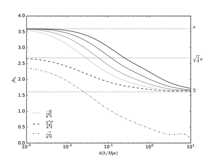
Figure 1: Sound speeds computed from the linearized Vlasov equation. Solid lines are computed with respect to the stress , $\Pi$, with darker lines indicating heavier neutrino mass. The dashed and dash-dotted lines are computed with respect to the pressure $k^{2}P$ and the anisotropic stress $\tau$ for $m_{\nu}=50$ meV. Horizontal dotted lines are pre-computed asymptotic behaviours which are independent of both neutrino mass and time. $\beta=m/(k_{B}T_{\nu}c)$.

We see that neutrinos are approximately bimodal with constant sound speed at large and small $k$. Both these values are computable. For $k\rightarrow 0$, $j_{0}(ku(s-s^{\prime})/\beta)\simeq 1$. This means the velocity integral becomes separable from the $s$ integral and we find

$$-\frac{\beta^{2}}{k^{2}}\Pi \simeq\int ds^{\prime}a^{2}(-k^{2}\phi)(s-s^{\prime})\sigma^{2}$$

$$\delta \simeq\int ds^{\prime}a^{2}(-k^{2}\phi)(s-s^{\prime})$$ (10)

$$\therefore c_{s}^{2} =\left(\frac{\sigma}{\beta}\right)^{2}$$

where $\sigma$ is the velocity dispersion $\sigma^{2}=\langle u^{2}\rangle_{0}\simeq 12.94$. For large $k$, the sinusoids in the velocity integral oscillate rapidly and add to zero unless $s^{\prime}\simeq s$ Ringwald and Wong (2004); Ali-Haimoud and Bird (2012). Under this assumption, $(a\delta_{m})(s^{\prime})\simeq(a\delta_{m})(s)$ and can be factored out of the integral yielding:

$$-\frac{\beta^{2}}{k^{2}}\Pi \simeq a^{2}(-k^{2}\phi)\left(\frac{\beta}{k}\right)^{2}$$

$$\delta \simeq a^{2}(-k^{2}\phi)\left(\frac{\beta}{k}\right)^{2}\Sigma^{-2}$$ (11)

$$\therefore c_{s}^{2} =\left(\frac{\Sigma}{\beta}\right)^{2}$$

where one must be particularly careful in changing the order of integration and $\Sigma$ is an “inverse dispersion” $\Sigma^{-2}=\langle u^{-2}\rangle_{0}\simeq 0.38$. This second sound speed is also the one that goes into defining the free streaming wavenumber $k_{fs}=\sqrt{\frac{3}{2}\Omega_{m}a}H_{0}\frac{\beta}{\Sigma}$. A simple “instantaneous” approximation on small scales is easily found by considering Eq. 6: for large $k$, $\delta_{ss}\ll c_{s}^{2}k^{2}\delta$ and so $\delta\simeq\frac{-a^{2}k^{2}\phi}{c_{s}^{2}k^{2}}$ or:

$$\delta\simeq\left(\frac{k_{fs}}{k}\right)^{2}\delta_{m}$$ (12)

on small scales. Equivalently, we can treat this as an equation for the sound speed:

$$c_{s}^{2}=\frac{\frac{3}{2}H_{0}^{2}\Omega_{m}a}{k^{2}}\frac{\delta_{m}}{\delta}.$$ (13)

Finally, we can divide the stress tensor into pressure, $P$, and anisotropic stress,$\tau$, $\Pi=-k^{2}P+\tau$. Equations for these components are again derived in the Supplement:

$$\beta^{2}P =\int_{-\infty}^{s}ds^{\prime}a^{2}(-k^{2}\phi)(s-s^{\prime})\frac{1}{3}\langle u^{2}(j_{0}(ku(s-s^{\prime})/\beta)+$$

$$\hskip 28.45274pt+2j_{1}(ku(s-s^{\prime})/\beta)/(ku(s-s^{\prime})/\beta)\rangle_{0}$$ (14)

$$-\frac{\beta^{2}}{k^{2}}\tau =\int_{-\infty}^{s}ds^{\prime}a^{2}(-k^{2}\phi)(s-s^{\prime})\frac{2}{3}\langle u^{2}(j_{0}(ku(s-s^{\prime})/\beta)$$

$$\hskip 28.45274pt-j_{1}(ku(s-s^{\prime})/\beta)/(ku(s-s^{\prime})/\beta)\rangle_{0}$$ (15)

We can now repeat our small scale approximations for these two components, e.g. $P/(\delta)$ and $\tau/(-k^{2}\delta)$. For the pressure on small scales, we expand the sinusoides to find $\frac{1}{3}(j_{0}(x)+2j_{1}(x)/x)\simeq\frac{5}{9}x$ and so the sound speed is $\sqrt{5/9}\sigma$. This result was derived by Shoji and Komatsu (2010). On small scales, repeating the above derivation shows that $k^{2}P\rightarrow\Pi$ and $\tau\rightarrow 0$. These approximations are shown as horizontal lines in Fig. 1 and closely match the integrated values (dashed and dash-dotted lines).

III.2 Perturbed Distribution Function

We now repeat the arguments used in computing the large and small scale sound speed limits but for the distribution function instead. Assuming negligible initial conditions, Eq. II.1 can be written as:

$$f(s,k,v,\mu)=\int_{-\infty}^{s}ds^{\prime}a^{2}ik\phi\mu\frac{df^{0}}{dv}e^{-ikv\mu(s-s^{\prime})}$$

where $\mu=\vec{k}\cdot\vec{v}/(kv)$. We can now integrate over angles to find:

$$\langle f(s,k,v)\rangle =\frac{1}{2}\int_{-1}^{1}d\mu f(s,k,v,\mu)$$

$$=\frac{df^{0}}{dv}\int_{-\infty}^{s}ds^{\prime}a^{2}k\phi j_{1}(kv(s-s^{\prime})).$$

In the large scale limit, $kv(s-s^{\prime})\ll 1$ and $j_{1}(kv(s-s^{\prime}))\simeq kv(s-s^{\prime})/3$. Using this approximation and substituting the density obtained in Eq. III.1 yields:

$$\langle f\rangle=-\frac{1}{3}v\frac{df^{0}}{dv}\delta.$$

In the small scale limit limit limit, we again use $s\simeq s^{\prime}$ and find

$$\langle f\rangle =\frac{df^{0}}{dv}a^{2}k\phi\int_{-\infty}^{s}ds^{\prime}j_{1}(kv(s-s^{\prime}))$$

$$=\frac{1}{v}\frac{df^{0}}{dv}a^{2}\phi\int_{0}^{\infty}j_{1}(x)dx$$

$$=-\frac{1}{v}\frac{df^{0}}{dv}\frac{\Sigma^{2}}{\beta^{2}}\delta$$

where we use the density in Eq. III.1 instead. This result was also computed in Ali-Haimoud and Bird (2012) using a different technique. We note now that strictly speaking these are not “low-k” and “high-k” limits, rather, they refer to limits where $kv\ll$ or $\gg(\Delta s)^{-1}$ for some timescale $\Delta s$. Nonetheless we will refer to the limits as such throughout the paper. Both the low- and high-k perturbations are separable in position and velocity and so we can define the velocity space perturbation as $f^{1}(v)=\langle f\rangle(v,k,s)/\delta(k,s)$. In terms of the dimensionless velocity $u=\beta v$ we have:

$$\bar{f}^{1}(u) =\frac{\langle f\rangle(u,k,s)}{\delta(k,s)}$$

$$=\frac{1}{u}\frac{e^{u}}{\left(e^{u}+1\right)}\bar{f}^{0}(u)\begin{cases}\frac{1}{3}u^{2}&ku(\Delta s)/\beta\ll 1\\ \Sigma^{2}&ku(\Delta s)/\beta\gg 1.\end{cases}$$ (16)

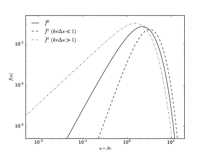
Figure 2: The unperturbed Fermi-Dirac distribution $\bar{f}^{0}(u)$ as a function of $u=\beta v$ is shown as a solid curve. The first order perturbations $\bar{f}^{1}(u)$ are shown as dashed (low-k limit) and dash-dotted (high k limit). Note that we include the $u^{2}$ part of $d^{3}u$ in the distributions. $\beta=m/(k_{B}T_{\nu}c)$

We plot $\bar{f}^{1}(u)$ in Fig. 2 and compare it to $\bar{f}^{0}(u)$. We see that the low-k limit tends to shift neutrinos to higher velocities; presumably due to the gravitational accelerations. This is qualitatively consistent with the velocity distributions seen in simulations, e.g. Fig. 4 and 13 of Villaescusa-Navarro et al. (2013). On the other hand, the high-k limit favours low velocity neutrinos and, to our knowledge, has not previously been seen. We have also been unable to find particles distributed this way in simple tests of our own simulations.

If neutrinos were distributed according to $\bar{f}^{1}(u)$ rather than $\bar{f}^{0}(u)$, the asymptotic sound speeds would change. For the $kv(\Delta s)\ll 1$ limit, the asymptotic values would be $\sqrt{\langle u^{2}\rangle_{1}}=\sqrt{5/3}\sigma$ at low-k and $1/\sqrt{\langle u^{-2}\rangle_{1}}=\sqrt{3}\Sigma$ at high k. For $kv(\Delta s)\gg 1$, the low-k asymptote becomes $\sqrt{\langle u^{2}\rangle_{1}}=\sqrt{3}\Sigma$; however, the high-k asymptote goes to zero. This is due to integrating from $u=0$, which clearly violates $ku(\Delta s)/\beta\gg 1$ regardless of k (the reverse case, for low-k, is less of a problem as $\bar{f}^{0}$ is truncating $u\rightarrow\infty$ and we can also simply consider $k=0$). Hence, the sound speed need not necessarily be zero as the approximation technique is somewhat inapplicable. Nonetheless, the high-k perturbation is more sensitive to low velocity neutrinos and therefore the asymptotic sound speed should decrease when including higher perturbations.

III.3 Simulation Sound Speed

Eq. 13 depends only on the total matter density field and the neutrino density field. We can therefore use our simulation power spectra to estimate the sound speed with the approximation $\delta(k)=\sqrt{\Delta^{2}(k)}$. We show the results in Fig. 3. We find that this estimate of the sound speed is significantly lower than the linear theory prediction of Eq. III.1 with values $\beta c_{s}\sim 1$ rather than $\sim\Sigma$. There is also now significant mass dependence of the asymptotic value, consistent with our expectation that heavier neutrinos should behave less linearly, and more like CDM (which has no sound speed).

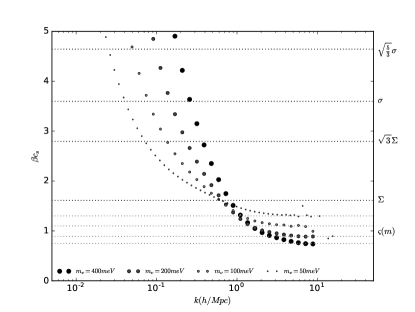
Figure 3: Estimates of the simulation sound speed for different neutrino masses. Dots are estimated using the instantaneous approximation (Eq. 13) and are valid only at high k. Lines show asymptotic values (note that $\varsigma$ is calibrated to the instantaneous approximation shown). $\beta=m/(k_{B}T_{\nu}c)$

With this behaviour we can now interpret the discrepency between linear response and N-body. The k-dependence of the sound speed is proportional to $\delta_{m}/(k^{2}\delta)$. By definition, $\delta_{m}$ is perfectly linear in $\delta_{m}$. Therefore, in order to drive the sound speed to lower values $\delta$ must be larger. This can only occur if, on small scales, non-linearities affect $\delta$ much more than they do $\Pi$. This makes sense as the $\Pi$ is weighted by $v^{2}$ as compared to $v^{0}$ for $\delta$. Hence, we expect Eq. 5 to be more accurate than Eq. 4 as high velocity neutrinos behave more linearly. Furthermore, a decrease in $c_{s}$ causes the density to grow more non-linearly, inducing feedback to continue decreasing $c_{s}$. Since low mass neutrinos are more linear in $\delta$, they are less affected by this instability and so their sound speed is closer to the linear theory asymptotic value, $\Sigma$.

III.4 Neutrino Power Spectrum

We show the neutrino power spectrum for $m_{\nu}=400$ meV in the top panel of Fig. 4. Black points correspond to the N-body results. Black dashed lines are linear response solutions, integrated against linear theory (lower curve) or with a non-linear correction: $\delta_{m}\rightarrow\delta_{m}\sqrt{P_{NL}/P_{L}}$ (upper curve). The dashed grey curve is the adiabatic approximation: $P_{\nu}=(T_{\nu}/T_{m})^{2}P_{NL}$. We see that it is a reasonably good fit to linear response. However, neither linear response or adiabatic solutions reproduce N-body results. This is despite the fact that the usual criterion for non-linearity, $\Delta^{2}(k)>1$, is not met on any scale. On the other hand, the grey curve shows the solution corresponding to Eq. 7, with a sound speed measured from Fig. 3, and agrees very well with N-body on small scales. Finally, we show asymptotic behaviour (e.g. Eq. 12) for linear and non-linear potentials as dotted lines.

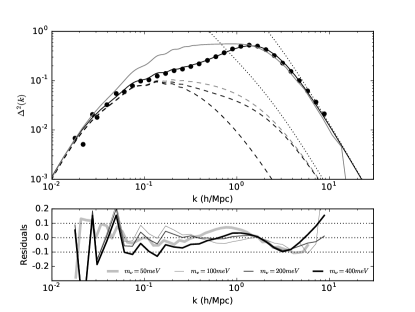
Figure 4: Top Panel Neutrino power spectrum at $z=0$ for $m_{\nu}=400$ meV. Dashed black lines indicate linear response to linear (lower curve) and HALOFIT (higher curve) potentials. The dashed grey line is the adiabatic approximation. The dots are from our N-body simulations. The solid grey curve corresponds to the sound speed solution chosen to match the high k behaviour. Dotted lines are asymptotic behaviours $\propto\delta_{m}/k^{2}$. Finally, the solid black line is our model. Bottom Panel Residuals between model and N-body for different neutrino masses.

We now present a simple model relating the neutrino power spectrum, $\Delta^{2}_{\nu}(k,z,m_{\nu})$ to the matter power spectrum, $\Delta^{2}_{m}(k,z,m_{\nu})$:

$$\Delta^{2}_{\nu}=\Delta^{2}_{m}\left[\frac{T_{\nu}}{T_{m}}+\left(\frac{k_{\beta}}{k}\right)^{2}\left(\frac{1}{\varsigma^{2}}-\frac{1}{\Sigma^{2}}\right)W(k/k_{\varsigma})\right]^{2}$$ (17)

where $T_{i}$ are linear transfer functions computed via a Boltzmann code such as CLASS, $k_{\beta}(z)=\Sigma k_{fs}=\sqrt{\frac{3}{2}\Omega_{m}a}H_{0}\beta$ is a typical fluid free-streaming scale neglecting the impact of the Fermi-Dirac distribution, $\beta c_{s}=\varsigma=\varsigma(z,m_{\nu})$ is the best fitting sound speed at high-k, and $W(k/k_{\varsigma})$ is a high pass filter that truncates the high-k accoustic behaviour.

We now explain each portion of the model. The factor of $T_{\nu}/T_{m}$ corresponds to linear behaviour under adiabatic initial conditions (which, as previously noted, is quite close to linear response when given the non-linear HALOFIT potential). The second term is the calibrated asymptotic behaviour at high-k, e.g. $\delta_{\nu}\propto\delta_{m}/k^{2}$ after subtracting out the linear behaviour (with $-1/\Sigma^{2}$). We compute $\varsigma=\beta c_{s}$ at redshift $z=0$ by averaging the last three points in Fig. 3. We know it must depend on time as it should go to its linear value, $\Sigma$, at high redshift. We compute $\varsigma$ for a few redshifts and show the results in the bottom subpanel of Fig. 5.

Figure 5: Top Panel N-body (dots), model (solid) and adiabatic (dotted) power spectra at redshifts $z=2.0,1.0,0.5,$ and $0.0$ for $m_{\nu}=200$ meV. Bottom Panel Redshift dependence of $\varsigma=\beta c_{s}$ evaluated at high k using the instantaneous approximation (Eq. 13) for a variety of redshifts and masses. At redshifts $z>2$ we are unable to resolve the value. Solid lines are for the model given in Eq. 18.

We model the behaviour as:

$$\varsigma(z)=\varsigma(0)+(\Sigma-\varsigma(0))Y(z)$$ (18)

where $Y(z)$ goes from $0$ at low redshift to $1$ at high redshift. We find $Y(z)=1-e^{-z/2}$ works reasonably well and is shown in the bottom panel of Fig. 5. Unfortunately we are unable to resolve the power spectra (and hence $\varsigma$) at high k for neutrinos below $200$ meV at higher redshifts. Finally, we find the following form for $W$ provides a good fit:

$$W(x)=\frac{1}{1+x^{-n}}$$ (19)

where $n$ must be $>2$ so that at small scales we recover linear behaviour. We find $n=2.25$ allows for good fits to all neutrino masses.

Thus, our model has one parameter that can be calibrated from simulations, $\varsigma(m_{\nu},z=0)$, one fitted parameter $k_{\varsigma}(m_{\nu})$, and two functions $W(k)$ and $Y(z)$, the former depending on $n=2.25$. We fit between $0.2<k/(\mbox{h}/\mbox{Mpc})<9$ (the lower bound is to avoid low-k variance) and tabulate these values at $z=0$ in Table 1.

Mass (meV)	50	100	200	400
$\varsigma=\beta c_{s}$	1.30	1.10	0.89	0.75
$k_{\varsigma}(\mbox{h}/\mbox{Mpc})$	1.11	0.92	1.20	1.65

Table 1: Parameters used in modeling the neutrino power spectrum. $\varsigma$ is the dimensionless sound speed calibrated from high-k measurements in N-body simulations. $k_{\varsigma}$ is a best fit parameter.

This model is shown as a solid black curve in Fig. 4 and residuals for all neutrino masses are shown in the bottom subpanel. We see that in regions $0.1<k/(\mbox{h}/\mbox{Mpc})<10$ our model is accurate to $~{}10\%$. Since we do not consider time dependence of $k_{\varsigma}$ (or $n$), at higher redshifts our model does not describe the simulated power spectra as well. For instance, for $m_{\nu}=400$ meV there is over $50\%$ difference at $z=0.5$. Nonetheless, this is still much better than linear response, as seen in the top panel of Fig. 5 where we show power spectra at various redshifts along with the adiabatic approximation for $m_{\nu}=200$ meV.

IV Discussion

Recently, Banerjee and Dalal (2016) performed numerical simulations treating neutrinos as a fluid. They evolved the density and velocity fields using the continuity and Euler equations and estimated the full position-dependent stress tensor from N-body neutrino particles. While this is the most accurate way to close the neutrino hierarchy equations, other possibilities exist including those discussed here.

In Fig. 3 we demonstrated that, on small scales, the non-linearity in the sound speed is due to the neutrino density, not its stress. In addition, on large scales the behaviour becomes more linear and the sound speed is unimportant as $j_{0}(kc_{s}(s-s^{\prime}))\simeq 1$. We speculate that it may be sufficient to close the hierarchy equations using an approach analagous to Ali-Haimoud and Bird (2012) but using linear response to compute $\Pi$ instead of $\delta$.

The benefits of such a scheme are significant compared to N-body. For instance, in our particle implementation there are $N^{3}$ neutrinos and $(N/2)^{3}$ CDM particles, each requiring six 4-byte floats. Hence, neutrinos are allocated $8/9$ of the available memory. On the other hand, in a grid based implementation there could be $N^{3}$ CDM particles, and two grids with $(N/2)^{3}$ cells each requiring one 4-byte integer. In this case neutrinos only require $4/100$ of the memory available. In addition, less computational time could be spent on neutrinos (due to the simplified hydrodynamic structure) and more time on the CDM. Finally, as in Banerjee and Dalal (2016), the neutrinos could be simulated starting at a high redshift (compared to our N-body implementation which starts them at $z\leq 10$). If the redshift is too high (e.g. above the neutrino relativistic to non-relativistic transition), this approach does not accurately describe neutrinos (which would be significantly relativistic) but the calculation would at least be self-consistent and such high redshift discrepencies are unlikely to propagate to late time effects. Despite these benefits, a dispersive fluid approach would require extensive comparisons to N-body results to calibrate the sound speed and validate the results.

V Conclusion

We have considered neutrinos as a dispersive fluid and found that this provides additional physical insights into their clustering behaviour. We have computed the sound speed and shown that it depends on the intial neutrino velocity distribution and also the non-linear cold dark matter. We find that the excess in power observed in the N-body neutrino power spectrum compared to linear response can be explained via a higher-order modification to the sound speed. Based on this, we have provided a simple model for the neutrino power spectrum that requires no additional integration beyond standard Boltzmann code outputs. Finally, we speculate that treating neutrinos as a dispersive fluid could allow for them to be simulated efficiently in both memory and processing time.

Supplement

V.1 Vlasov Moments

We describe a simple trick to computing $\delta=\frac{\int d^{3}vf}{\int d^{3}vf^{0}}$, $\theta=ik^{i}\frac{\int d^{3}vv^{i}f}{\int d^{3}vf^{0}}$ and $\Pi=-k^{i}k^{j}\frac{\int d^{3}vv^{i}v^{j}f}{\int d^{3}vf^{0}}$. Instead of computing each moment separately, we instead compute a “Moment Generating Function” - the Fourier transform in velocity space of the distribution function. That is,

$$M(s,k,h)=\frac{\int d^{3}ve^{-ih^{i}v^{i}}f(s,k,v)}{\int d^{3}vf^{0}(v)}$$

where the moments can now be computed by taking derivatives - e.g. $\delta=M(s,k,0)$, $\theta=k^{i}\left(\frac{\partial M}{\partial h^{i}}\right)_{h=0}$, $\Pi=k^{i}k^{j}\left(\frac{\partial^{2}M}{\partial h^{i}\partial h^{j}}\right)_{h=0}$ Substituting Eq. II.1 in yields:

$$M =\int ds^{\prime}a^{2}ik^{i}\phi\frac{\int d^{3}ve^{-iv^{j}(h^{j}+k^{j}(s-s^{\prime}))}f^{0}_{v^{j}}(v;\beta)}{\int d^{3}vf^{0}(v;\beta)}$$

$$=\int ds^{\prime}a^{2}(-k^{i}g^{i}\phi)\frac{\int d^{3}vf^{0}(v;\beta)e^{-v^{j}g^{j}}}{\int d^{3}vf^{0}(v;\beta)}$$

where we integrated by parts and defined $g^{i}=h^{i}+k^{i}(s-s^{\prime})$. The angular part of the velocity integral can be performed explicitly by taking the angle between $v^{j}$ and $g^{j}$ to be the polar angle. This yields $\int_{-1}^{1}d\mu_{vg}e^{ivg\mu_{vg}}=2j_{0}(vg)$. Using this result and rearranging yields:

$$M =\int ds^{\prime}a^{2}(-k\phi)\frac{\int dvv^{2}f^{0}(v;\beta)g\mu_{kg}j_{0}(vg)}{\int dvv^{2}f^{0}(v;\beta)}$$

$$=\int ds^{\prime}a^{2}(-k\phi)\langle g\mu_{kg}j_{0}(ug/\beta)\rangle_{0}$$ (20)

where $\mu_{kg}$ is the angle between $k^{j}$ and $g^{j}$ and $u=\beta v$. We can immediately find the density in Eq. 4 by taking $g=k(s-s^{\prime})$ and $\mu_{kg}=1$. In order to obtain the other moments we need to differentiate. This can be conveniently performed since $g^{j}\propto h^{j}$ and so $L=k^{j}\partial/\partial h^{j}=k^{j}\partial/\partial g^{j}$. In spherical coordinates this becomes: $L=k\mu_{kg}\frac{\partial}{\partial g}+k\frac{1-\mu_{kg}^{2}}{g}\frac{\partial}{\partial\mu_{kg}}$ where we use the fact that $M$ only depends on $\mu_{kg}$. For $\theta$ and $\Pi$ this further simplifies since we always take $\mu_{kg}=1$ and so we only need: $L=k\frac{\partial}{\partial g}$. Applying $L$ and $L^{2}$ to Eq. V.1 straightforwardly gives the velocity divergence, $\theta=ik^{i}\langle v^{i}\rangle$, and Eq. 5. In summary:

$$\delta =\int ds^{\prime}a^{2}(-k^{2}\phi)(s-s^{\prime})\langle j_{0}(ku(s-s^{\prime})/\beta)\rangle_{0}$$ (21)

$$-\theta =\int ds^{\prime}a^{2}(-k^{2}\phi)\langle\cos(ku(s-s^{\prime})/\beta)\rangle_{0}$$ (22)

$$-\frac{\beta^{2}}{k^{2}}\Pi =\int ds^{\prime}a^{2}(-k^{2}\phi)(s-s^{\prime})\langle u^{2}j_{0}(ku(s-s^{\prime})/\beta)\rangle_{0}.$$ (23)

To compute the pressure it is slightly easier to simply start from the definition:

$$3P =\Pi^{ii}=\frac{\int d^{3}vv^{i}v^{i}f}{\int d^{3}vf^{0}}$$

$$=\int_{-\infty}^{s}ds^{\prime}a^{2}ik^{i}\phi\frac{\int d^{3}vv^{2}e^{-ik^{j}v^{j}(s-s^{\prime})}f^{0}_{v^{i}}(v;\beta)}{4\pi\int dvv^{2}f^{0}(v;\beta)}$$

$$=\int_{-\infty}^{s}ds^{\prime}a^{2}ik\phi\frac{\int d\mu dvv^{2}f^{0}(v;\beta)(-2v\mu+ik(s-s^{\prime})v^{2})e^{-ik^{j}v^{j}(s-s^{\prime})}}{2\int dvv^{2}f^{0}(v;\beta)}$$

$$=\int_{-\infty}^{s}ds^{\prime}a^{2}ik\phi\frac{\int dvv^{2}f^{0}(v;\beta)v^{2}(ik(s-s^{\prime})j_{0}(kv(s-s^{\prime}))+2j_{1}(kv(s-s^{\prime}))/v)}{\int dvv^{2}f^{0}(v;\beta)}$$

$$=\int_{-\infty}^{s}ds^{\prime}a^{2}(-k^{2}\phi)(s-s^{\prime})\langle u^{2}(j_{0}(ku(s-s^{\prime})/\beta)+2j_{1}(ku(s-s^{\prime})/\beta)/(ku(s-s^{\prime})/\beta)\rangle_{0}.$$

We can now expand $\Pi=(ik^{i})(ik^{j})\Pi^{ij}$ in terms of the pressure and the anisotropic stress: $\Pi=-k^{2}P+\tau$ and by comparison with Eq. 5 and the above equation for the pressure find

$$\beta^{2}P =\int_{-\infty}^{s}ds^{\prime}a^{2}(-k^{2}\phi)(s-s^{\prime})\frac{1}{3}\langle u^{2}(j_{0}(ku(s-s^{\prime})/\beta)+$$

$$\hskip 28.45274pt+2j_{1}(ku(s-s^{\prime})/\beta)/(ku(s-s^{\prime})/\beta)\rangle_{0}$$ (24)

$$-\frac{\beta^{2}}{k^{2}}\tau =\int_{-\infty}^{s}ds^{\prime}a^{2}(-k^{2}\phi)(s-s^{\prime})\frac{2}{3}\langle u^{2}(j_{0}(ku(s-s^{\prime})/\beta)$$

$$\hskip 28.45274pt-j_{1}(ku(s-s^{\prime})/\beta)/(ku(s-s^{\prime})/\beta)\rangle_{0}.$$ (25)

V.2 Fluid Green’s Functions

Eq. 6 is simply a driven harmonic oscillator:

$$\delta_{ss}+\omega^{2}\delta=S(s,k)$$

with $\omega=c_{s}k$ and $S(s,k)=a^{2}(-k^{2}\phi)$. We can define a Green’s function $G(s,s^{\prime})$ via:

$$\delta =\int ds^{\prime}G(s,s^{\prime})S(s^{\prime})$$

$$=\int ds^{\prime}G(s,s^{\prime})(\delta_{s^{\prime}s^{\prime}}+\omega^{2}\delta)$$

$$=[G\delta_{s^{\prime}}-G_{s^{\prime}}\delta]_{-\infty}^{s}+\int ds^{\prime}(G_{s^{\prime}s^{\prime}}+\omega^{2}G)\delta$$

$$\therefore G_{s^{\prime}s^{\prime}}+\omega^{2}G=\delta_{D}(s-s^{\prime})$$

and we have the freedom to choose the Green’s function boundary conditions so as to eliminate the surface term: $G=G_{s^{\prime}}=0$ for $s^{\prime}>s$. This has the solution:

$$G =A\sin(\omega s^{\prime})+B\cos(\omega s^{\prime});s^{\prime}<s$$

$$=0;s^{\prime}>s.$$

Continuity at $s=s^{\prime}$ requires $B=-A\tan(s)$ and the jump condition $\int_{s-\epsilon}^{s+\epsilon}ds^{\prime}[G_{s^{\prime}s^{\prime}}+\omega^{2}G=\delta_{D}(s-s^{\prime})]$ yields $-G_{s^{\prime}}(s)=1$ indicating $A=\cos(ws)/w$ and $B=-\sin(ws)/w$. Combining these two yields the Green’s function:

$$G(s-s^{\prime})=(s-s^{\prime})j_{0}(\omega(s-s^{\prime}))$$

and so, for the gravitational source, we find

$$\delta =\int ds^{\prime}a^{2}(-k^{2}\phi)(s-s^{\prime})j_{0}(kc_{s}(s-s^{\prime})).$$

$\theta$ is easily computable through $\theta=-\delta_{s}$:

$$\theta=\int ds^{\prime}a^{2}(-k^{2}\phi)\cos(kc_{s}(s-s^{\prime})).$$