Discreteness Effects in Simulations of Hot/Warm Dark Matter

Abstract

In Hot or Warm Dark Matter universes the density fluctuations at early times contain very little power below a characteristic wavelength related inversely to the particle mass. We study how discreteness noise influences the growth of nonlinear structures smaller than this coherence scale in $N$-body simulations of cosmic structure formation. It has been known for 20 years that HDM simulations in which the initial uniform particle load is a cubic lattice exhibit artifacts related to this lattice. In particular, the filaments which form in such simulations break up into regularly spaced clumps which reflect the initial grid pattern. We demonstrate that a similar artifact is present even when the initial uniform particle load is not a lattice, but rather a glass with no preferred directions and no long-range coherence. Such regular fragmentation also occurs in simulations of the collapse of idealised, uniform filaments, although not in simulations of the collapse of infinite uniform sheets. In HDM or WDM simulations all self-bound nonlinear structures with masses much smaller than the free streaming mass appear to originate through spurious fragmentation of filaments. These artificial fragments form below a characteristic mass which scales as $m_{p}^{1/3}k_{peak}^{-2}$, where $m_{p}$ is the $N$-body particle mass and $k_{peak}$ is the wavenumber at the maximum of $k^{3}P(k)$ ($P(k)$ is the power spectrum). This has the unfortunate consequence that the effective mass resolution of such simulations improves only as the cube root of the number of particles employed.

1 Introduction

In the absence of a full analytic understanding of nonlinear structure growth, numerical simulations provide a critical link between the weak density fluctuations measured in the cosmic microwave background and the strong inhomogeneities observed on all but the very largest scales in the present Universe. Indeed, numerical simulations played a decisive role in excluding massive neutrinos as a dark matter candidate (White et al., 1983) and in establishing the $\Lambda$CDM model as the leading and now standard paradigm for the formation of all structure (Davis et al., 1985; White et al., 1987; Cen et al., 1994; Navarro et al., 1996). With the development of more powerful computer hardware, of more accurate numerical algorithms, and of methods to follow additional physical processes, the importance of simulations as a tool to interpret observations of observed structure continues to increase dramatically. In this paper we are concerned with one aspect of the simplest kind of cosmological structure formation simulation, namely how discreteness effects can drive the growth of spurious small-scale structure in N-body simulations of evolution from initial conditions containing no such structure.

To create initial conditions for a cosmological simulation, a uniform particle distribution is needed. This can be perturbed by a random realisation of the linear fluctuation field associated with the specific structure formation model to be simulated (e.g. $\Lambda$CDM). A uniform Poisson distribution of particle positions is not suitable for this purpose, because stochastic “root-$N$” fluctuations can exceed the density fluctuations predicted by the desired model over a wide range of scales. To avoid this problem, most early simulations chose a regular cubic lattice as the initial uniform load. Symmetry then assures that there can be no growth of structure in the absence of imposed perturbations (Efstathiou et al., 1985). The preferred directions and the large-scale coherence of the lattice may, however, be a disadvantage, since they can give rise to numerical artifacts. As an alternative, White (1996) suggested using a glass-like initial particle load created by carrying out a cosmological simulation from Poisson initial conditions but with the sign of the peculiar gravitational accelerations reversed, so that each particle is repelled by all the others. When such a system reaches quasi-equilibrium, the total force on each particle vanishes, as for a grid, but there are no preferred directions and no long-range order. The power spectrum on scales much larger than the mean interparticle spacing approaches a power-law $P(k)\sim k^{n}$ with $n=4$ (Baugh et al. 1995), where $n=4$ is the minimal large-scale power expected for a discrete stochastic system (Peebles, 1980, section 28).

Normally, grid and glass initial loads are considered equivalent. Nevertheless, artifacts due the initial lattice are obvious in early images of the sheets, filaments and “voids” formed in Hot Dark Matter (HDM) simulations (e.g. Centrella & Melott, 1983; Frenk et al., 1984; Efstathiou et al., 1985; Centrella et al., 1988). Baugh et al. (1995) and White (1996) showed that low density regions appear very different in simulations with a grid initial load than in simulations started from a glass, although Baugh et al. found that this does not show up as a difference in their power spectra. Nevertheless, the regularly spaced clumps seen along filaments in HDM simulations are clearly related to the initial particle grid, and so seem unlikely to reflect a true physical instability. Despite this, Bode et al. (2001) and Knebe et al. (2003) interpreted analogous structures in their Warm Dark Matter (WDM) simulations (which were set up using a grid initial load) as the result of the physical fragmentation of filaments. The nonlinear formation of such small-scale structure could have important consequences in models like HDM or WDM where power on small scales is strongly suppressed in the linear initial conditions. It is thus important to establish which simulated structures are real and which are artifacts, as well as to understand whether the simulations can be improved by, for example, choosing a glass initial load in place of a grid.

Götz & Sommer-Larsen (2002, 2003) carried out WDM simulations using both grid and glass initial loads and reported significant differences. With a grid they found spurious low-mass halos evenly spaced along filaments, exactly as in earlier HDM experiments. The spacing is simply that of the initial grid, stretched or compressed by the large-scale distortion field. They emphasised, however, that such unphysical halos were less evident in their simulations starting from a glass. This conclusion disagrees with our own work below, where we find spurious halos also in simulations from glass initial conditions and with a frequency very similar to that found in the grid case. Curiously, in the glass case also we find the spurious halos to be regularly spaced along filaments even though the initial condition is not regular over the relevant scales.

In this paper, we wish clarify this issue by isolating the numerical artifact, by exhibiting it in idealised filament formation simulations, by exploring its dependence on the nature of the uniform particle load, and by establishing the dependence of its characteristic scale on the discreteness scale of the simulation and the coherence scale of the WDM/HDM initial conditions. We carry out cosmological simulations of an HDM universe at a wide range of resolutions and with both grid and glass initial loads. In addition, we simulate the collapse of an infinite straight uniform density filament from glass initial conditions, showing that it fragments into regularly spaced clumps. To gain additional insight, we also consider the collapse of a glass to a uniform sheet, and the growth of structure in a uniform, space-filling, but anisotropically compressed glass. Rapid fragmentation on small scales occurs only in the filament case. Our tests also demonstrate that considerable care is needed to produce an initial glass load for which the growth of small-scale structure in filaments is optimally suppressed. We propose a randomisation technique which successfully washes out most code-dependent periodic signals in the initial load.

The remainder of our paper is organised as follows. In $\S 2$ we first discuss the aspects of our simulation code which are relevant to the problem at hand, in particular, how it estimates gravitational accelerations and how it is modified in order to create a uniform glass distribution. We then describe the way in which initial conditions are created for the simulations presented in the rest of the paper. $\S 3$ presents results from our Hot Dark Matter simulations, showing that all small-scale collapsed structures appear to form initially as regularly spaced clumps along filaments, and that these are similar for grid and for glass initial loads. Results for our studies of idealised structure formation from anisotropically compressed glasses are presented in $\S 4$. Rapid fragmentation on small scales occurs only in the filament case. $\S 5$ examines this filament fragmentation in more detail, showing that its characteristic scale is related to the interparticle separation for a well-constructed glass, but that scales related to the Poisson-solver of the glass-construction code can play an important role if their influence is not carefully controlled. Finally, $\S 6$ summarises the implications of our results for simulations of structure formation. In particular, we show that for nonlinear structures the effective mass resolution of simulations of HDM or WDM universes improves only as the cube root of the number of simulation particles employed. This is much more pessimistic than the direct proportionality to $N$ which might naively have been expected.

2 Simulation methods and initial conditions

All simulations in this paper were performed using the massively parallel N-body code L-Gadget2. This is a lean version of Gadget2 (Springel, 2005) with the SPH part excluded and with the memory requirements minimised. It was originally written in order to carry out the Millennium Simulation (Springel et al., 2005).

The computation of gravitational forces is the most critical and time-consuming element of any cosmological $N$-body code. Gadget2 uses a hybrid tree-PM method where the long-range force is calculated at low resolution using a particle-mesh scheme, and is supplemented by a high-resolution but short-range correction calculated using a tree algorithm. The short-range correction is assembled in real space by collecting contributions from all neighbouring particles. The long-range force is calculated by assigning the particles to a regular cubic mesh, by using Fourier methods to obtain the corresponding potential, and by numerically differencing the result. For a single particle this scheme introduces a maximum force error of 1-2 percent near the split scale. Choosing a suitable split scale (typically several times the mean interparticle separation) results in force errors for smooth distributions of particles which are almost everywhere far below 1 percent. Gadget2 uses a space-filling fractal, the Peano-Hilbert curve, to control the domain decomposition associated with parallelisation. Because there is a good correspondence between the spatial decomposition obtained from this self-similar curve and the hierarchical tree used to compute forces, it is possible to ensure that the tree decomposition used by the code is independent of the platform, in particular of the number of processors on which it is run. In addition, the “round-off” errors in the forces induced when summing contributions from all processors are explicitly considered. As a result, the forces are independent of the number of processors and the domain cuts that are made. We believe that all code-related numerical effects relating to the calculation of gravitational accelerations are well under control in Gadget2.

Glass construction is embedded in Gadget2 by using some compile options. A preset number of particles is initially distributed at random within the cubic computational volume and the standard scheme is used to obtain the gravitational acceleration on every particle. After reversing the signs of the accelerations, all particles are advanced for a suitably chosen timestep. The velocities are then reset to zero and the whole procedure is repeated. After about a hundred steps the acceleration of each particle approaches zero. Notice that this is the acceleration as obtained by the code, including the effects of force anisotropy, domain decomposition, etc. Because the glass is made in a periodic cube, we can get a large glass file cheaply by tiling a big box with many replications of the original glass. However, the accelerations calculated by the code may no longer vanish exactly for this larger glass because the force anisotropies and inaccuracies now occur on a different scale than when the glass was created.

The FFT calculation and the Barnes & Hut tree used in Gadget2 are both based on static grids. This spatially fixed decomposition introduces weak periodic signals in the force calculation, and these are reflected in the particle distribution at the end of the glass-making procedure. We will see below that that this can introduce measurable spikes in the 1-D power spectrum of the final glass. To reduce such effects we randomly offset the particle distribution in all three coordinates with respect to the computational box before carrying out each force computation during glass-making. This suppresses the induced signals quite effectively but does not fully eliminate them. A glass constructed in this fashion is referred to as a “good” glass in the following, while a glass constructed without the random offset technique and showing significant high spikes is referred to as a “poor” glass. In the rest of this paper, we use “good” glasses for our initial conditions except where explicitly noted. These issues are further discussed in section 5.

Below we consider grid initial loads in addition to glasses in order to compare their performance and to check the results of previous work (Bode et al., 2001; Götz & Sommer-Larsen, 2002, 2003). A third quasi-uniform particle distribution, the Quaquaversal distribution, has recently been suggested by Hansen et al. (2007) as a non-periodic uniform initial load, a possible alternative to a glass. We have created such a Quaquaversal load with $2\times 8^{7}$ particles using the code provided by Hansen et al at their web site, and we compare its performance to our grid and glass initial loads in an Appendix. It produces significantly worse discreteness artifacts than either grids or glasses.

Two types of simulation are considered below. The first is a series of cosmological simulations of evolution from Hot Dark Matter (HDM) initial conditions. Most of these are for a single realisation of the HDM density field within a 100$h^{-1}$Mpc cube, but with different kinds of initial load and with varying mass resolution. One considers a 200$h^{-1}$Mpc cube in order to better constrain the abundance of large objects. For these simulations, we choose an Einstein-de Sitter universe dominated by a single massive neutrino. We take $H_{0}=76.5{\rm kms^{-1}Mpc^{-1}}$ which implies a neutrino mass of $\sim 55{\rm eV}$ and a corresponding free-streaming scale $\lambda=22.2~{}{\rm Mpc}$ (Bond & Szalay, 1983) below which initial fluctuations are exponentially suppressed relative to an assumed $P(k)\propto k$ primordial power spectrum. The power spectrum we actually use to impose fluctuations on our initial loads is based on the theoretical predictions of Bardeen et al. (1986) and agrees with numerical estimates from the Boltzmann solver CMBFAST (Seljak & Zaldarriaga, 1996). Since the same realisation is used for all our 100$h^{-1}$Mpc simulations, they should all produce identical structures. We start integrating at redshift $z=20$ and evolve structure to a formal present-day amplitude of $\sigma_{8}=2$. This corresponds to the collapse of the first nonlinear structure in the simulation at $z\sim 6$. As a check of our starting redshift we reran one simulation glass128 starting from $z=100$. At $z=15$ the power spectrum of this simulation differed from that of the original run by few percent or less on all scales.

Our simulations are listed with their parameters in Table 1: pre-IC, L, $m_{p}$, $\epsilon$,and $n_{p}$ denote the initial load, the box size, the particle mass, the softening length, and the particle number respectively.

Table 1: HDM simulations

name	$pre-IC$	$L[h^{-1}{\rm Mpc}]$	$m_{p}[h^{-1}M_{\odot}]$	$\epsilon(h^{-1}{\rm Mpc})$	$n_{p}$
glass64	glass	100	$1.06\times 10^{12}$	0.08	$64^{3}$
glass128	glass	100	$1.32\times 10^{11}$	0.04	$128^{3}$
glass256	glass	100	$1.65\times 10^{10}$	0.02	$256^{3}$
glass256-2	glass	200	$1.32\times 10^{11}$	0.04	$256^{3}$
glass512	glass	100	$2.07\times 10^{9}$	0.01	$512^{3}$
grid128	grid	100	$1.32\times 10^{11}$	0.04	$128^{3}$
qset134	Q-set	100	$1.32\times 10^{11}$	0.04	$\sim 134^{3}$

Our second type of simulation is designed specifically to study the discreteness artifacts which show up in the filamentary structures within our HDM simulations. These simulations follow evolution from a variety of highly idealised initial conditions, all based on uniformly but anisotropically compressed glasses. We consider three different cases:

Anisotropic glass: The glass initial load is compressed by a factor of 2 along one axis, by a factor of 3 along a second axis, and is unaltered along the third axis. Six replications of this configuration are then used to tile the computational cube to produce an initial condition which is uniform and glass-like on large scales but where the forces are no longer balanced on the scale of the interparticle separation.

Sheet: The glass initial load is compressed along one dimension by a factor of 2, so that it fills half of the computational volume. The other half remains empty. This configuration collapses to form an infinite uniform sheet.

Filament: Our glass initial load is compressed by a factor of 2 along two of its periodic directions while the third remains unchanged. The particles then fill a quarter of the computational volume, the rest remaining empty. This configuration collapses to form a uniform straight filament.

All the simulations carried out from these initial conditions assume an Einstein-de Sitter background universe. We define the expansion factor $a$ to be unity at the initial time.

We identify collapsed “halos” in our HDM simulations using a Friends-of-Friends (FOF) algorithm with linking length 0.2 times the mean interparticle spacing (Davis et al 1985). In the following we will only consider FOF halos with 32 or more particles. Subhalos within these halos were identified using the SUBFIND algorithm (Springel et al., 2001) with parameters set to retain all overdense self-bound regions with at least 20 particles. Based on these subhalo catalogues we use the techniques of Springel et al. (2005) to construct merging trees which allow us to follow the formation and evolution of all halos and subhalos.

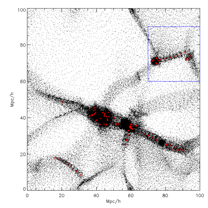
Figure 1: A slice of thickness $10h^{-1}{\rm Mpc}$ through the HDM simulation glass128 at $z=0$. Small black points indicate individual simulation particles, while the larger red points show FOF halos with $32\leq N_{fof}<300$.

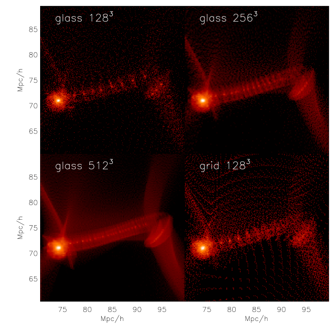
Figure 2: A subregion containing a filament at $z=0$ in four of our $100h^{-1}$Mpc HDM simulations based on differing initial loads and differing mass resolution. The first three panels are taken from glass$128$, glass$256$ and glass$512$ respectively, while the last one ( bottom right) is taken from grid$128$. The region shown here corresponds to that surrounded by a blue square in Fig 1.

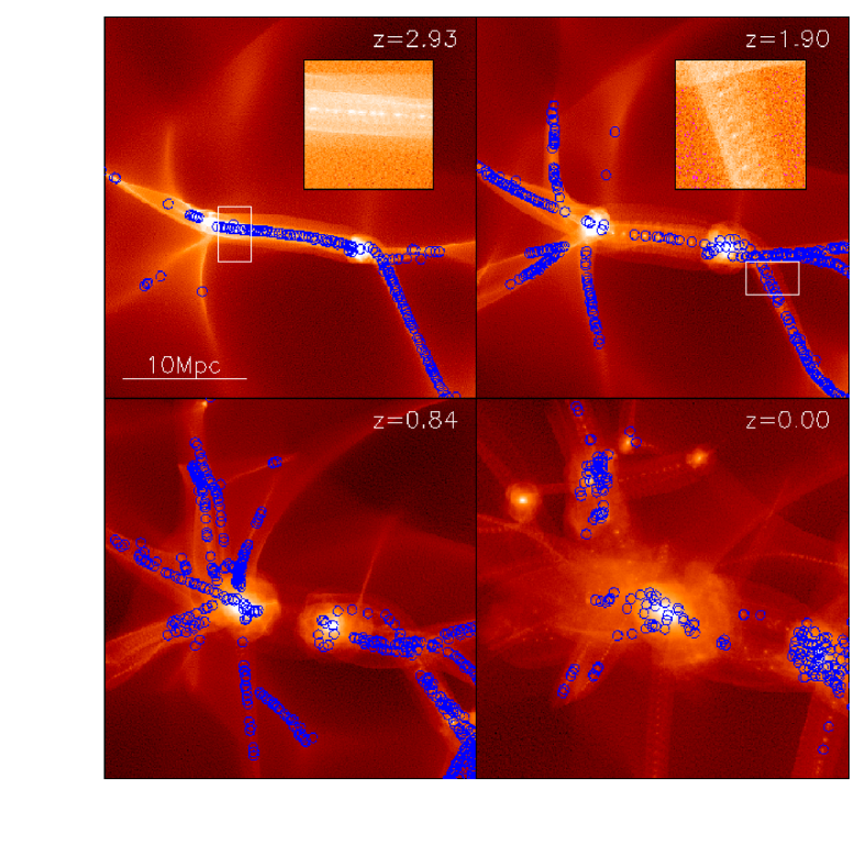
Figure 3: The bottom right panel shows a subregion of glass512 at $z=0$ containing the largest FOF halo. The blue circles indicate all subhaloes with more than 20 particles within this object. The other three panels show the same subregion at earlier times ($z=0.84;1.90;2.93$) with the blue circles now indicating the progenitors of all subhaloes identified at $z=0$. It is striking that almost all these progenitors lie in 1-D structures — filaments — at the earlier times. The two smaller plots in the upper panels are stretched and magnified images of the filaments indicated by white rectangles in the main panels.

3 Filament Fragmentation in HDM Simulations

The original motivation for this paper came from an unexpected phenomenon in our HDM simulations. Even when we use a glass initial load, we find that the filaments in these simulations break up into regularly spaced clumps, just as in early simulations based on grid initial loads. We illustrate this in Fig. 1 which shows a slice through simulation glass128. All FOF haloes with $32\leq N_{fof}<300$ are indicated by red points. It is obvious that many of these low-mass haloes lie in the filaments, and that they are surprisingly regularly spaced along them.

We find similar behaviour in all our HDM simulations, independent of the initial load and the mass resolution. In Fig. 2 we focus on a small cubic subregion containing a filament. (This region is indicated by a blue square in Fig. 1). In all four simulations, small clumps are visible at regularly spaced positions along the filament. Their spacing is very similar in the two $128^{3}$ simulations, even though one started from a glass and the other from a grid. The spacing is reduced by about a factor of two in the $256^{3}$ simulation and by about another factor of two in the $512^{3}$ simulation. The clumps are difficult to see in this last case, but this is merely a consequence of the resolution of the image (compare Fig. 3 below). There are strong indications that these clumps are a numerical artifact, not least because in the grid128 case they line up with the distorted but still recognisable pattern of the initial grid, just as in early HDM simulations (e.g. Centrella & Melott 1983) or in the WDM simulations of Götz & Sommer-Larsen (2003). Götz & Sommer-Larsen (2003) reported that the effect is absent when starting from a glass, although their Fig. 1 appears to show it in the filament at the lower right corner of their image. Bode et al. (2001) also noticed that many low-mass haloes formed in the filaments of their WDM simulation, but they interpreted this as a result of physical pancake fragmentation. The tight relation between clump scale and mass resolution manifest in Fig. 2 makes it clear, however, that this is actually a reflection of N-body discreteness effects. Its surprising aspect is that the regular clump spacing persists in the glass case where the initial load has no large-scale coherence. We consider this issue further below.

Another consequence of this artifact is illustrated in Fig. 3. It appears that almost all the subhaloes within the massive objects present at $z=0$ actually originated through spurious filament fragmentation. Fig. 3 focusses on a small subregion of the glass512 simulation which contains the largest FOF halo, an object with several linked density centres at $z=0$. The lower right panel shows the final mass distribution in this cubic region. All subhaloes with SUBFIND particle count greater than 20 are indicated by blue circles. The other three panels use our merging trees to trace all progenitors of these subhaloes back to earlier times. All of them appear to form initially as evenly spaced “beads” strung along filaments. They later fall into the large halo where they are seen at $z=0$. The artificial regularity of their formation is illustrated by the two zooms in the upper panels. We conclude that the first generations of haloes in pure HDM or WDM universes should contain no dark matter subhaloes of smaller mass scale.

4 Structure Growth in Idealised Glass Collapses

In our HDM simulations there is very little power in the imposed HDM power spectrum below the free-streaming scale. The regular fragmentation of the filaments is clearly related to the mesh for a grid initial load, but the origin of the equally regular fragmentation in the glass case is less obvious. In Fig.4 we analyse the structure of a “good” $160^{3}$ particle glass to search for signs of unexpected periodic behaviour. The irregular blue line in this figure is the dimensionless 3-D power per unit $\ln k$, $\Delta^{2}(k)=k^{3}P_{3}(k)$ where $P_{3}(k)$ is the 3-D power spectrum. For comparison, the straight blue line gives the expectation for a Poisson distribution with the same number of particles ($P(k)=1/N$). On large scales the power in the glass is far below this white noise level, with $\Delta^{2}(k)\propto k^{7}$ rather than $\Delta^{2}(k)\propto k^{3}$. For a relatively narrow frequency band near $k=160$, however, the power is noticeably above the Poisson expectation. This corresponds approximately to the separation of the clumps which form on the filaments so there may be some connection to this artifact in our HDM simulations.

Fig. 4 also shows the power per unit $\ln k$ in 2-D and 1-D projections of this same glass, $\Delta^{2}(k)=k^{2}P_{2}(k)$ and $\Delta^{2}(k)=kP_{1}(k)$ respectively. Again the measured results are compared to the expectation for a Poisson distribution with the same number of particles. Both cases show features directly analogous to those seen in the 3-D power spectrum. On large scales (small $k$) the power is strongly suppressed relative to the white noise level, with a spectrum which is steeper than white noise by four powers of $k$. Near $k=160$ there is a narrow range of wavenumbers where the power rises significantly above the white noise level. Again this feature could be related to the break up of sheets or filaments into clumps spaced regularly at about the mean interparticle separation.

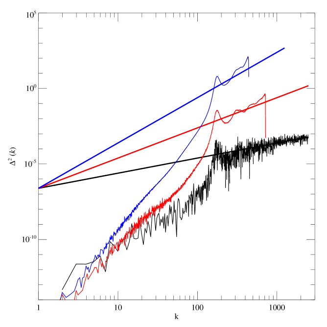
Figure 4: The 1-D (black), 2-D (red) and 3-D (blue) dimensionless power per unit $\ln k$ for a glass with $160^{3}$ particles. The straight lines are the corresponding expectations for a Poisson distribution of $160^{3}$ particles. The wavenumber $k$ is given in natural units so that k=1 corresponds to the fundamental mode of the computational cube. The glass used here is a “good” glass, where random position offsets at each timestep were used to suppress artifacts due to anisotropies in the Gadget2 Poisson solver (see section 5).

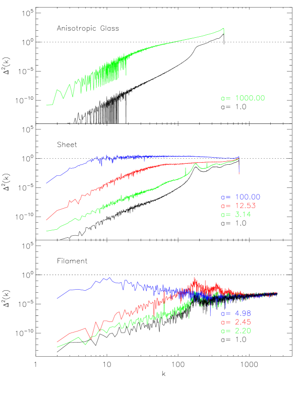
Figure 5: The evolution of the power per unit $\ln k$ in three idealised simulations. Top: the 3-D power at the initial time and after expansion by a factor of 1000 for an anisotropically compressed but space-filling glass. Centre: the 2-D power at the initial time and after expansion by factors of 3.1, 12.5 and 100 for the 1-D collapse of a compressed glass to a sheet. First collapse occurs at $a=3.1$. Bottom: the 1-D power at the initial time and after expansion by a factors of 2.2, 2.4 and 5 for the 2-D collapse of a compressed glass to a filament. Here first collapse occurs at $a=2.2$.

Whether these features can indeed explain the unexpected fragmentation of filaments in our HDM simulations depends, of course, on how they are amplified as the particle distribution evolves. For the first structures to collapse in an HDM universe, this evolution can be idealised as a succession of three phases (Zel’dovich, 1970). During early nonlinear growth, the tidal field causes a locally anisotropic flow which first reverses along a single preferred direction while continuing to expand (although at different rates) along the two orthogonal directions. In the second phase, collapse along the preferred axis gives rise to a quasi-two-dimensional sheet-like structure, a “pancake”. Collapse along one of the other two axes then produces a filament. Finally, material flows along filaments to produce dark matter haloes at their intersections. These features are all clearly visible in Fig. 1, although in practice the different phases overlap and interact significantly. In Fig. 5 we show the results from a set of idealised simulations of anisotropic collapse designed to explore how discreteness noise grows for a glass initial load during these various phases.

To illustrate structure growth in the first of the above phases, the top panel of Fig. 5 shows the evolution of the total 3-D power per $\ln k$ for evolution from an anisotropically compressed, but space-filling and otherwise unperturbed glass. (It is easier for us to simulate the isotropic expansion of an anisotropically distorted glass than the anisotropic expansion of an initially isotropic glass.) The $160^{3}$ “good” glass of Fig. 4 was here compressed by a factor of 2 along the $x$-axis and a factor of 3 along the $y$-axis, then replicated 6 times in order to tile the full simulation cube. The exact periodicities introduced by this procedure are responsible for the regular gaps in power visible at low $k$ in the initial power histogram (the black curve in Fig. 5). It is interesting that the “bump” in power at the discreteness scale is broader than in Fig. 4 and now stretchess from near $k=160$, the interparticle separation of the original glass past $k\sim 300$, the interparticle separation of the compressed glass. Clumping during expansion from this initial condition is extremely slow. The green curve shows the power distribution after expansion by a factor of 1000. By this time the matter has aggregated into small dense knots which typically contain 50 particles, but on larger scales the distribution remains almost uniform. At long wavelengths the power has grown by about six orders of magnitude, just as predicted by linear theory. Thus the characteristic mass of the clumps grows as $M_{*}\propto a^{6/7}$. The amplification of discreteness noise is very weak during the first phase of anisotropic evolution from glass initial conditions.

The second panel of Fig. 5 studies the growth of discrete noise during and after collapse to a sheet. We compress our $160^{3}$ glass by a factor of 2 along one axis, leaving the other half of the simulation cube empty. This initial condition collapses to a thin uniform sheet and thereafter remains thin with the particles oscillating about the symmetry plane. The figure shows the total 2-D power per $\ln k$ in the projection of particle distribution onto this plane at four different times: the initial time, the moment when the mass first collapses to a thin configuration ($a=3.1$), the moment the sheet reaches minimum thickness for the second time ($a=12.5$) and a substantially later time ($a=100$). In this case the power on large scales grows much faster than in the previous case with $\Delta^{2}$ increasing approximately as $a^{6}$ rather than as $a^{2}$. At the time of first collapse, the power in the discreteness peak has grown rather little, even though the power on larger scales has already amplified substantially. By the time of second collapse many nonlinear clumps are already evident in the projected mass distribution and the feature at the scale of the initial interparticle separation is no longer visible in the power spectrum. The characteristic nonlinear scale is determined by the point where the amplified long wavelength $\Delta^{2}\propto k^{6}$ tail crosses $\Delta^{2}\sim 1$. This scale increases rapidly with time, approximately as $M_{*}\propto a^{3}$. Structure in a pancake thus grows by an accelerated version of the standard hierarchical aggregation mechanism illustrated in a more familiar context in the top panel of Fig. 5. Discreteness effects do not appear to play a role other than by setting the initial amplitude of the long wavelength tail of $\Delta^{2}(k)$.

The lowest panel of Fig. 5 shows similar data for an idealised simulation of collapse to a filament. We compress our $160^{3}$ glass by a factor of 2 along two orthogonal axes, leaving the remaining three quarters of the simulation cube empty. This bar-like initial condition collapses to a thin, straight filament. The figure shows the 1-D power per $\ln k$ for the projection of the particle distribution onto the axis of the filament at four different times: the initial time, the time of first collapse ($a=2.2$), a time shortly thereafter ($a=2.4$) and a significantly later time ($a=5$). The power spectra here are considerably noisier here than in the top two panels because there are far fewer modes per bin in $\ln k$. By first collapse the large-scale power has grown substantially but there is rather little amplification near the discreteness peak at $k\sim 160$. This is similar to the sheet case. Shortly after first collapse, however, the power in the discreteness peak has grown by a large factor, reaching nonlinear levels. This shows up as regular clumping along the filament with a periodicity close to $k=160$. It differs from the behaviour in the sheet case and is apparently analogous to the filament fragmentation we saw in our HDM simulations. We investigate it further in the next section. After the filament collapses the large-scale tail of the power distribution amplifies extremely rapidly, roughly as $\Delta^{2}\propto a^{20}$. At the last time plotted this growth is again setting the nonlinear scale, as in the upper two panels, and there is no obvious feature near $k=160$.

In all three of these tests the scale of nonlinearity at late times reflects the amplified small-$k$ tail of the initial power spectrum of the glass. This tail grows much more rapidly in a sheet than in a uniform 3-D distribution and much more rapidly in a filament than in a sheet. The initial glass, if well made, does exhibit the theoretical minimum power on large scales $P(k)\propto k^{4}$ (Zel’dovich 1965; Peebles 1980), so that no better suppression of discreteness effects can be hoped for. In the filament case, however, the first nonlinear structures are clearly different in nature and are related to the interparticle separation scale of the uncompressed glass. We now consider this instability more closely.

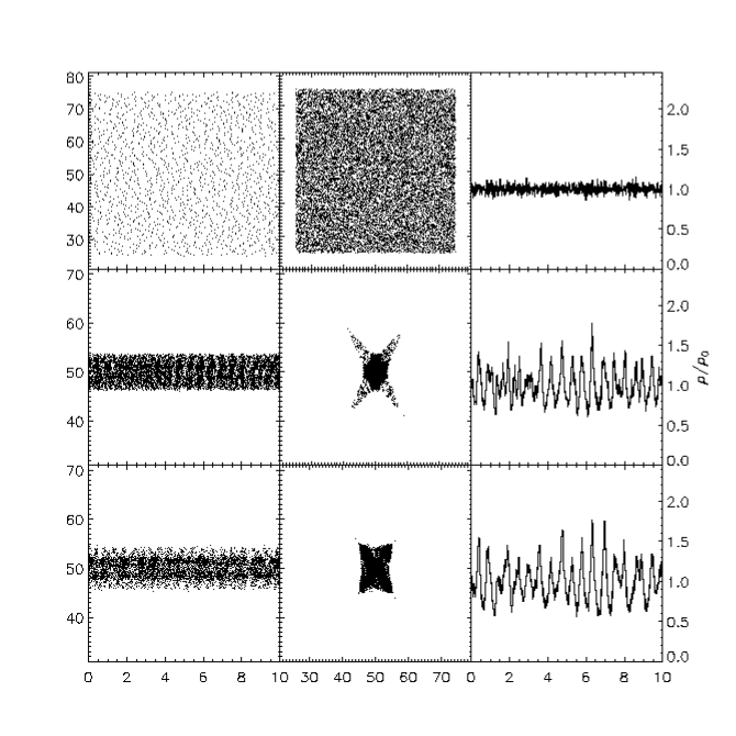
Figure 6: The evolution of an idealised infinite straight filament. The first and second columns are views perpendicular to and along the filament. Comoving coordinates are here normalised so that the side of the computational cube is 100. The third column is the 1-D number density profile along the filament. The density is normalised to unity and overdensities should be read off against the scale on the right-hand-side of the plot. Results are shown for expansion factors $a=1,2.4$ and 2.6, from top to bottom. For clarity only $1/10$ of the whole filament is shown here. In fact, the total number of clumps lying along the filament is about 160.

5 Fragmentation of filaments

In Fig. 6 we illustrate the evolution of the collapsing filament discussed in the last section. The first and second columns show projections perpendicular to and along the filament, while the third shows its 1-dimensional projected density. Only a tenth of the full length of the filament is plotted in order to make its structure more visible. Shortly after $a=2$ the filament collapses to minimum thickness and at almost the same time it breaks up into regularly spaced clumps. The clump spacing is very nearly equal to the mean interparticle separation in the unperturbed glass; we find $\sim 160$ clumps along the full length of the filament. The number of clumps is independent of the FFT grid used. For $128^{3}$, $243^{3}$, $400^{3}$ FFT grids, we find the total number of lumps to be always around $\sim 160$. Furthermore, we have repeated this fragmentation experiment with different compression factors in the initial condition. This changes the time of first collapse but it changes neither the fact that the filament breaks up just after first collapse, nor the spacing of the clumps. The same is true even if we adopt different compression factors along the two axes (provided both are well above unity) or if we impose an initial perturbation which is axially symmetric and has no sharp edges. Using an initial glass with a different number of particles produces a change in the interclump separation which scales as the cube-root of $N$. Clearly then, the break up is associated with a feature of the unperturbed glass.

The regular spacing of these artifacts indicates that modes with $k\sim N^{1/3}$ dominate at least the early nonlinear evolution of structure along the filament. This is visible in the left panels of Fig. 7, which repeat the power spectra at the initial time and at $a=2.4$ (just after collapse) from Fig. 5. At the initial time the power around $k\sim 160$ is more than three orders of magnitude below the threshold for nonlinearity, but by $a=2.4$ it is already approaching unity and is well above the power on all the other scales plotted. This is the reflection in Fourier space of the remarkable regularity seen in Fig. 6. The lower left panel of Fig. 7 plots growth factors for individual modes between the two times. The fastest growing modes have $k$ somewhat smaller than 100, but their growth is insufficient for them to overtake the initial power peak near $k\sim 160$. The power in all the modes in this peak grows by a similar amount so the peak remains relatively narrow. This causes the regular spacing of clumps along the filament. Tests with a $270^{3}$ particle glass show identical behaviour but with the peak shifted to $k\sim 270$. We conclude that the regularly spaced clumps which form on the filaments of our HDM simulations are produced by a narrow peak in power near the mean interparticle separation of our initial glass load. This peak is amplified to nonlinearity by the remarkably rapid growth of structure which occurs once a filament has collapsed.

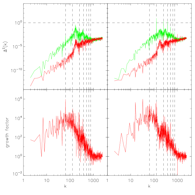
Figure 7: The top panels show the evolution of the 1-D power spectra corresponding to the simulations in Fig. 6 (a “good” glass: left) and Fig. 8 (a “poor” glass: right) which differ only in the initial glass used. The red curves represent the initial conditions ($a=1$) while the green curves represent $a=2.4$. The bottom panels show the growth factors between the two times plotted mode by mode. Note that these reach values in excess of $10^{6}$. The dashed black vertical lines indicate modes $k=64,128,256,384,512,640,768$. It can be seen that the growth factors are anomalously high for these modes in both panels, and that in the case of the “poor glass” a number of them are also anomalously high in the initial condition. As a result, at the later time the structure along the filament is dominated in the latter case by the modes with $k=128,256$ and 384.

Careful examination of Fig. 7 shows that there are particular modes for which the growth appears anomalously strong, notably those with $k=64,128,256,384...$. This is very likely a consequence of anisotropies in Gadget’s Poisson solver which is based on a binary decomposition of the computational volume. For the “good” glass used here these modes do not grow enough to overtake the power in the peak associated with the interparticle separation, so it is the latter which determines the initial fragmentation scale of the filament. We now show that this is not always the case.

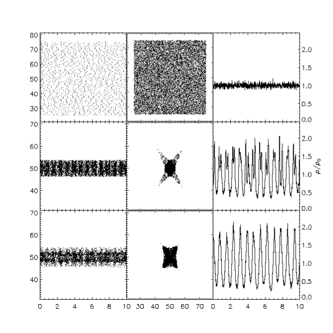
Figure 8: Similar to Fig. 5. but starting from a “poor” glass where the initial 1-D power spectrum shows spikes at $k=64,128,256..$. There are about 128 clumps along the full length of the filament at the last time shown.

Up to this point all our results have been based on such a “good” initial glass for which the offset technique discussed in §2 was used to minimise features due to anisotropies in the force calculations. Nevertheless, artifacts due to force anisotropies are still visible in some of our plots. For example, spikes can be seen in Fig. 5 at $k=128$ and 256 in the $a=3.1$ power spectrum of the sheet (these spikes are solely due to modes with wave-vector parallel to the fundamental axes of the computational cube) and at $k=64$ and 256 in the $a=2.4$ power spectrum of the filament (see also the left panels of Fig. 7). The growth factors in Fig. 7 show that these “special” modes grow substantially more rapidly than neighboring modes. If we do not use random offsets to reduce the impact of algorithmic boundaries in the force calculation, then features of this kind can be strong enough in the initial glass to significantly affect later evolution. An example is shown in the right panels of Fig. 7 and also in Fig. 8. Here we have carried out exactly the same filament collapse test as before, but using a “poor” initial glass constructed without using the offset technique. Spikes are now visible at $k=128,256$ and $384$ in the initial 1-D power spectrum. These are amplified by the evolution and at $a=2.4$ the power is dominated by the amplified spike at $k=128$ rather than by modes in the neighborhood of the discreteness peak at $k\sim 160$. Spikes at $k=256$ and 384 are also very strong and several other spikes are clearly visible. As Fig. 8 shows, these spikes cause the filament to break up initially into $\sim 128$ rather than $\sim 160$ clumps. Subsequent aggregation into larger objects is similar in the two cases, however, with large-scale effects overwhelming the initial differences.

Eliminating these troublesome power spikes from the initial conditions and from subsequent evolution is not easy. Changing the nominal accuracy of the force calculation affects the amplitude of the spikes but does not remove them. We were surprised to find that similar spikes are present in the initial glass used for the GIF simulations (Kauffmann et al., 1999) even though this was created using a different code based on a $\rm{P^{3}M}$ Poisson solver. (For the GIF simulations the artifact was of no consequence, because of the substantial small-scale power imposed in the CDM initial conditions.) The large-scale PM force calculation in both codes imposes a regular “power of 2” spatial structure, and for Gadget-2 this is reinforced by the static Barnes-Hut oct-tree which underlies the calculation of the short range forces. The unexpected spikes appear to reflect these structural properties of the force construction algorithms. To test this, we projected the initial glass onto periodic directions which are not aligned with the axes of the computational box. The corresponding 1-D power spectra do not show any sharp spikes.

The tests in this section demonstrate that even with our random offset procedure artifacts due to our Poisson solver are not entirely eliminated. On the other hand, these tests are extremely sensitive to such artifacts because of the very high growth rates which occur in the idealised straight filaments we have been studying. While it is clearly important to be aware of the possibility of such numerical effects when simulating WDM or HDM universes, our results here show that for a carefully constructed glass the effects due to the Poisson solver remain subdominant with respect to effects caused by the discreteness of the particle distribution. The latter cannot be eliminated for any choice of initial particle load. They set the fundamental lower limit to the effective resolution of such simulations

6 Discussion and Conclusions

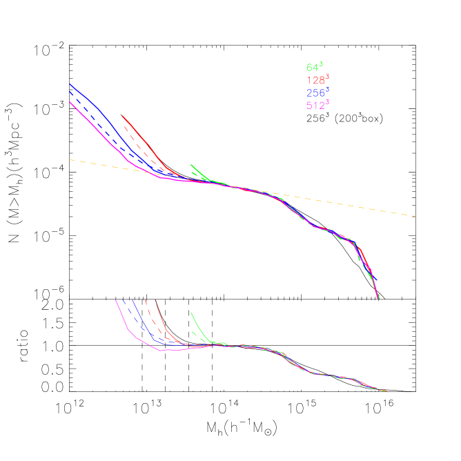
Figure 9: The cumulative halo mass function in eight simulations of an HDM universe. Seven of these start from the same realisation of the HDM density fluctuation field within a $100{\rm Mpc/h}$ box, but use different initial particle loads. One follows evolution within a $200{\rm Mpc/h}$ box in order to better constrain the high mass end of the mass function. Simulations starting from a glass initial load are indicated by solid lines, while those starting from a grid are indicated by dashed lines. The number of particles in each simulation is indicated by labels in the upper panel. The dotted line in this panel is an approximate power-law fit to the low-mass end of the mass function, $\rm N\sim M_{h}^{-0.2}$, and the lower panel replots the mass functions relative to this power law in order to emphasise the upturn due to discreteness effects. Dashed vertical lines separated by factors of two provide a rough indication of the scale where spurious halos start to dominate in the various cases. The haloes here were identified using an FOF algorithm with $b=0.2$ (Davis et al 1985).

In this paper we have studied how discreteness effects limit the effective mass resolution of $N$-body simulations of cosmogonies like WDM or HDM where structure on small scales is suppressed in the linear initial conditions. Filaments occur in such models as part of the natural development of the cosmic web, but in simulations they fragment into regularly spaced clumps with a separation which reflects the mean interparticle distance in the initial load. These spurious clumps are responsible for all the low-mass substructures we have been able to identify at late times in collapsed halos. Thus, it appears that in an idealised WDM or HDM universe the first generations of dark haloes are predicted to contain no self-bound substructures of significantly smaller scale. Our tests on idealised systems show this fragmentation to occur because 1-D projections of a 3-D quasi-uniform particle distribution retain substantial power on the scale of the 3-D interparticle separation, and this power amplifies very rapidly as the effectively 1-D system evolves.

We find (in disagreement with Götz & Sommer-Larsen (2002, 2003)) that spurious fragmentation of filaments occurs in almost identical fashion whether the initial particle load is a glass or a grid. Indeed, as we illustrate in Fig. 9, the effect appears slightly worse for a glass than for a grid. This plot gives mass functions for 9 simulations from HDM initial conditions which use different particle numbers and different initial loads. In each case there is a sharp upturn in abundance at small masses which reflects the clumps visible within filaments in Figures 1 to 3. For initial loads of a given type this upturn shifts to smaller masses by a factor of 2 for each factor of 8 increase in the number of particles. For a given number of particles the upturn clearly occurs at somewhat larger masses in the glass case than in the grid case. Notice also that the upturn for the $N=256^{3}$ glass simulation in a $200h^{-1}{\rm Mpc}$ box agrees very well with that for the $N=128^{3}$ glass simulation in a $100h^{-1}{\rm Mpc}$ box. This confirms that it is the mean interparticle separation which sets the mass scale, rather than properties of the simulation code or of the particular HDM realisation simulated.

If we take the effective lower resolution limit of our HDM simulations to be given by the dashed vertical lines in the lower panel of Fig. 9, we find that it can be expressed as $M_{lim}=10.1\times\bar{\rho}~{}d~{}k_{peak}^{-2}$, where $\bar{\rho}$ is the mean density of the universe, $k_{peak}$ is the wavenumber at the maximum of $\Delta^{2}(k)$, the dimensionless power per $\ln k$ in the linear initial conditions, $d=N^{-1/3}L$ is the mean interparticle separation, $N$ is the number of simulation particles, and $L$ is the side of the computational box. For our HDM initial conditions $k_{peak}=4.23\times\lambda_{fs}^{-1}=0.1\times(m_{\nu}/30eV){\rm Mpc}^{-1}$. The coefficient in our expression for $M_{\rm lim}$ is estimated directly from our HDM results. It may depend significantly on the shape of the primordial power spectrum and so need modification for WDM initial conditions. The scaling $M_{\rm lim}\propto N^{-1/3}$ should still hold in this case, however. Comparing our formula without modification to the numerical results of Bode et al. (2001) using $k_{peak}=1.0$ and $0.5~{}{\rm Mpc}^{-1}$, as appropriate for their two WDM models, gives $M_{\rm lim}=3\times 10^{10}$ and $1.2\times 10^{11}h^{-1}{\rm M_{\odot}}$. These values agree well with the upturns in the mass functions which they plot in their Fig. 9.

We can also compare with the WDM simulations presented by Knebe et al. (2002, 2003). These authors followed Bode et al. (2001) in arguing that small mass haloes form along filaments by top-down fragmentation. However, if we compare the mass functions they present for three different simulations in Fig. 4 of Knebe et al. (2002) and Fig. 3 of Knebe et al. (2003), we find the upturn at low mass for the two simulations with the same numerical resolution but different WDM particle mass to occur at masses which differ by about a factor of 4, while the upturn for the two runs with different numerical resolution but the same WDM particle mass also occur at masses differing by a factor of about 4. This is in roughly agreement with the scaling we predict for $M_{\rm lim}$ and is unexpected for a physical (rather than numerical) feature. We conclude that these results, as well as those of Bode et al. (2001) are consistent with a spurious numerical origin for the low mass halos in filaments similar to that we find in our HDM simulations. Furthermore, with our parametrisation of the characteristic scale based on the wavenumber at the peak of $\Delta^{2}(k)$, the dependence of the characteristic mass of the effect on the overall shape of the power spectrum appears to be weak.

This effective resolution limit is unfortunate news for simulations of HDM and WDM universes. In our highest resolution HDM model, for example, the $N=512^{3}$ glass simulation of a $100{\rm Mpc/h}$ box, the resolution limit is $M_{lim}=8.8\times 10^{12}h^{-1}{\rm M_{\odot}}$, which corresponds to a clump of $4300$ simulation particles. Thus only halos with $5000$ particles or more can be considered reliable. This is two or three orders of magnitude below the masses of typical big halos in the simulation. Contrast this with simulations of CDM universes where the positions, velocities and masses of haloes are reasonably well reproduced even for objects with about 100 simulation particles, giving a logarithmic dynamic range which is about twice as large. Furthermore the effective dynamic range in halo mass increases in proportion to $N$ for CDM simulations, but only in proportion to $N^{1/3}$ in HDM or WDM simulations.

These results are interesting for the question of whether WDM models can reproduce the observed properties of dwarf satellite galaxies in the Milky Way. Available kinematic data for dwarf spheroidals suggest that they are sitting in dark matter halos with maximum circular velocities of order 30 km/s (e.g. Stoehr et al., 2002; Kazantzidis et al., 2004) corresponding to masses (for an isolated object) of about $10^{10}{\rm M_{\odot}}$. After discounting the spurious low-mass halos, the mass functions shown in Fig. 9 of Bode et al. (2001) demonstrate that halos of such small mass are not expected for a WDM particle mass of 175 eV and are still strongly suppressed relative to $\Lambda$CDM for a mass of 350 eV. We infer that WDM particle masses well in excess of 500 eV will be necessary to produce “Milky Way” halos with sufficient substructure to host the observed satellites. This is, however, less stringent by a factor of several than constraints based on structure in the Lyman $\alpha$ forest (Viel et al., 2006). It will be interesting to carry out simulations of sufficient resolution to test whether the internal structure of subhalos in a WDM universe is consistent with that inferred for the halos of Milky Way dwarfs. The resolution limitations we have explored in this paper imply that, although possible, this will be a major computational challenge.

Appendix A The Quaquaversal distribution

Hansen et al. (2007) have suggested using an initial particle load constructed through a simple “Quaquaversal” tiling of space (sometimes known as a Q-set). In particular, they suggested using this initial load for WDM simulations. In this appendix, we show what happens if this distribution is used instead of a grid or glass initial load in a number of the tests we have studied in our paper.

A Q-set “lives” in a rectangular box with side ratio $1:1:\sqrt{3}$, and requires a total particle number of the form $N=2\times 8^{n}$ with $n$ an integer. Periodic boundary conditions can be assumed on opposite faces of the box to represent an infinite cosmological distribution. Fig. A1 compares the 3-D power spectrum of such a distribution with that of our “good” $160^{3}$ glass. This Q-set has $n=7$, resulting in a total of $N=4194304$ particles, and was set up using the codes provided by Hansen et al. (2007). In order to facilitate the comparison we shift $P(k)$ for the Q-set so that its white noise level is at $160^{-3}$ and the mode number $k=1$ corresponds to a wavelength 160 times the mean interparticle spacing. At all scales significantly larger than the mean interparticle spacing, the power in the Q-set lies well above that in the glass. The mean power declines approximately as $k^{3.4}$ for small $k$ rather than as $k^{4}$, and there is substantial power in a series of additional narrow peaks separated by factors of 2 in $k$.

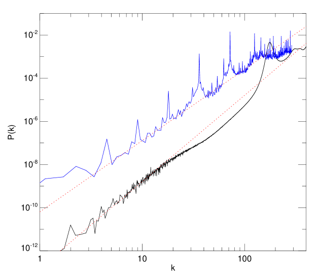
Figure 10: 3-D power spectra $P(k)$ for a Q-set (black) and for the “good” $N=160^{3}$ glass already used in Fig. 4 (blue). The Q-set has 4194304 particles in a rectangular box. Its power spectrum is normalised so that its white noise level is at $160^{-3}$, just as for the glass. In addition, the units of wave number are chosen so that $k=1$ corresponds to a wavelength 160 times the mean interparticle separation for both distributions. Red dotted lines indicate power laws with slope 4 and 3.4 which are good fits to the glass and Q-set power spectra respectively on large scales.

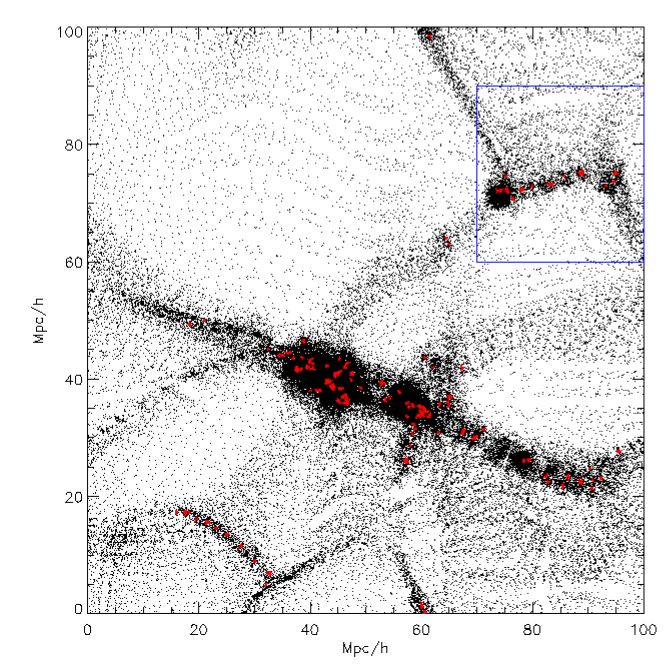
Figure 11: A slice through an HDM simulation directly comparable to Fig. 1, but for a simulation with a Q-set initial load.

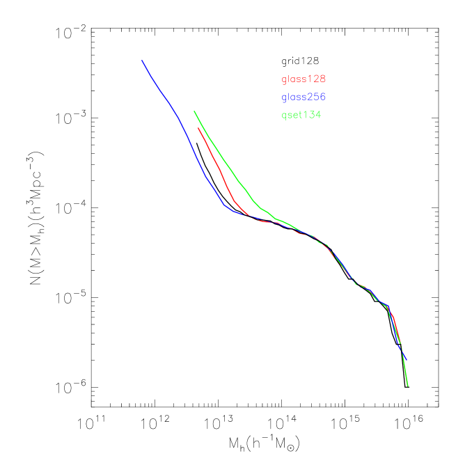
Figure 12: Mass functions for FOF haloes in four HDM simulations started from identical realisations of the HDM fluctuation field but with different initial particle loads. Two start from glass loads with $N=128^{3}$ (red) and $N=256^{3}$ (blue) and one starts from a grid with $N=128^{3}$. All three of these were already shown in Fig. 9. The final simulation starts from a Q-set initial load with $N\simeq 134^{3}$.

We have used this Q-set as the initial particle load for our standard $100h^{-1}{\rm Mpc}$ box HDM simulation. Since this simulation is carried out in a cubic region we need to chop off the long end of the Q-set rectangular box leaving a total of $2424140\sim 134^{3}$ particles in the simulation. This truncation results in a violation of periodicity in the initial load for one pair of faces of the cubic volume. As a result, spurious small clumps form along this interface during later evolution, but these effects do not propagate into the rest of the simulation. They are not visible in Fig. A2, which is a slice through the simulation to be compared directly with Fig. 1. We exclude a thin slice of the simulation which contains this discontinuity when we calculate the halo mass function at $z=0$. This is displayed in Fig. A3 and compared to our earlier results.

Figure 13: Idealised filament collapse as in Fig. 6 but starting from a compressed Q-set initial condition. The distribution of particles in a section of the filament is shown at $a=2.2$ and should be compared directly with the middle left panel of Fig. 6.

A comparison of Fig. A2 with Fig. 1 shows that the regularities of the Q-set are much more visually apparent than those of the glass, particularly in low density regions. The small halos indicated by red points are again found along filaments and on the outskirts of massive objects. Figure A3 shows that the Q-set reproduces the halo mass function of our other simulations at high mass, but that the turn-up due to spurious low-mass halos occurs at significantly higher mass than for glass or grid initial loads. The effective mass resolution of the Q-set simulation is about a factor of three worse than in either of the other cases.

We have also carried out our standard idealised filament simulation starting from a compressed Q-set rather than a compressed glass. The particle distribution along a section of the filament is shown just after collapse in Fig. A4 for comparison with the central left-hand panel of Fig. 6. Substantial and regular clumping is seen, although the regularity is considerably more complex (and also stronger) than in the glass case. As in the glass case, the clumps rapidly aggregate into a small number of massive objects during later evolution. The different initial power spectra of the glass and Q-set cases (Fig. A1), result in different rates of growth of structure along the filament at later times. Structures are always more massive are arranged in a more complex pattern along the filament for Q-set than in the glass case.

Our conclusion from these tests is that for given particle number the Q-set performs significantly worse as an initial load than either a grid or a glass. Since the visual regularities it induces are very similar to those seen for a grid and are much stronger than those found with a glass, there does not seem to be any obvious situation where a Q-set would be the preferred choice for an initial quasi-uniform particle load.

References

- Bardeen et al. (1986) Bardeen J. M., Bond J. R., Kaiser N., Szalay A. S., 1986, ApJ, 304, 15
- Baugh et al. (1995) Baugh C. M., Gaztanaga E., Efstathiou G., 1995, MNRAS, 274, 1049
- Bode et al. (2001) Bode P., Ostriker J. P., Turok N., 2001, ApJ, 556, 93
- Bond & Szalay (1983) Bond J. R., Szalay A. S., 1983, ApJ, 274, 443
- Cen et al. (1994) Cen R., Miralda-Escudé J., Ostriker J. P., Rauch M., 1994, ApJ, 437, L9
- Centrella & Melott (1983) Centrella J., Melott A. L., 1983, Nature, 305, 196
- Centrella et al. (1988) Centrella J. M., Gallagher III J. S., Melott A. L., Bushouse H. A., 1988, ApJ, 333, 24
- Davis et al. (1985) Davis M., Efstathiou G., Frenk C. S., White S. D. M., 1985, ApJ, 292, 371
- Efstathiou et al. (1985) Efstathiou G., Davis M., White S. D. M., Frenk C. S., 1985, ApJS, 57, 241
- Frenk et al. (1984) Frenk C. S., White S. D. M., Davis M., 1984, in Setti G., Van Hove L., eds, Large-Scale Structure of the Universe Elementary Particles and the Large-Scale Structure of the Universe - Short Contributions. pp 257–+