Precision reconstruction of the dark matter-neutrino relative velocity from N-body simulations.

Abstract

Discovering the mass of neutrinos is a principle goal in high energy physics and cosmology. In addition to cosmological measurements based on two-point statistics, the neutrino mass can also be estimated by observations of neutrino wakes resulting from the relative motion between dark matter and neutrinos. Such a detection relies on an accurate reconstruction of the dark matter-neutrino relative velocity which is affected by non-linear structure growth and galaxy bias. We investigate our ability to reconstruct this relative velocity using large N-body simulations where we evolve neutrinos as distinct particles alongside the dark matter. We find that the dark matter velocity power spectrum is overpredicted by linear theory whereas the neutrino velocity power spectrum is underpredicted. The magnitude of the relative velocity observed in the simulations is found to be lower than what is predicted in linear theory. Since neither the dark matter nor the neutrino velocity fields are directly observable from galaxy or 21 cm surveys, we test the accuracy of a reconstruction algorithm based on halo density fields and linear theory. Assuming prior knowledge of the halo bias, we find that the reconstructed relative velocities are highly correlated with the simulated ones with correlation coefficients of 0.94, 0.93, 0.91 and 0.88 for neutrinos of mass 0.05, 0.1, 0.2 and 0.4 ${\rm eV}{}$. We confirm that the relative velocity field reconstructed from large scale structure observations such as galaxy or 21 cm surveys can be accurate in direction and, with appropriate scaling, magnitude.

I Introduction

Despite extensive research in the particle physics and cosmology communities, many properties of neutrinos remain elusive. For instance, neutrino oscillation experiments (Fogli et al., 2012) have accurately measured the mass-squared splittings between neutrino species, but individual neutrino masses have yet to be measured. It is also unknown whether the neutrino masses follow a normal hierarchy in which there are two light neutrinos and a single heavy one or an inverted hierarchy with the opposite configuration. Moreover, it is still unknown whether neutrinos are Dirac or Majorana fermions.

Cosmological techniques for determining neutrino masses are currently insensitive to individual neutrinos and instead constrain the sum of all neutrino masses. For instance, cosmic microwave background (CMB) observations made by the Plank satellite place $\sum m_{\nu}<0.194\ {\rm eV}$ (Planck Collaboration et al., 2015). Recently, a new technique for constraining neutrino mass using large-scale velocity fields was proposed in (Zhu et al., 2014a, b). Neutrinos and dark matter are expected to have a relative velocity arising due to the free streaming of neutrinos over large scales. As neutrinos bulk flow over large scale structures they become focussed into wakes. Such downstream overdensities introduce a unique dipole distortion in the matter field in the direction of the neutrino flow which could be observed via either direct lensing of the wake or through a dipole component of the correlation function.

Unlike other probes of cosmological neutrinos, this method is expected to be background free and only relies on knowledge of the relative velocity field. Determining velocity fields directly is particularly challenging even for luminous matter and certainly impossible for neutrinos. However, the relative velocity is predicted to be coherent over several megaparsecs. We therefore expect linear theory to be accurate enough to allow for a reconstruction of the velocity field from the easier to obtain matter density field.

Our goal is to quantify the accuracy of this linear reconstruction when non-linear structure formation, which affects both the density and velocity fields, is taken into account. We furthermore wish to understand whether the reconstruction procedure is robust when only a tracer of the dark matter field is used. To achieve this we use large cosmological simulations. Neutrinos have been implemented in a variety of ways within the framework of N-body simulations: (i) (Brandbyge and Hannestad, 2009) used a grid-based approach where an additional neutrino density field is evolved alongside N-body dark matter; (ii) (Brandbyge and Hannestad, 2010) employed a hybrid method where neutrinos start as a grid and are converted to particles as their energy decreases; (iii) (Bird et al., 2012) evolved neutrinos as distinct N-body particles; (iv) (Ali-Haïmoud and Bird, 2013) computed the neutrino linear response alongside the evolving dark matter. In general, the grid-based approaches have been unable to resolve non-linear neutrino structure formation while particle-based approaches are hindered by the requirement that many neutrino particles are needed to reduce Poisson noise on small scales. In this work, we adopt the particle based approach since an accurate computation of non-linear neutrino dynamics is a main focus of our work.

In §II we discuss our implementation of neutrino particles into the cosmology code CUBEP³M (Harnois-Déraps et al., 2013) and our method for computing density and velocity fields. In §III we present the results of our simulations and analyse the accuracy of various reconstruction methods. In §IV we discuss a practical procedure to estimate cosmic velocity fields from density tracers.

II Theory and Implementation

II.1 Neutrino N-body Particles in CUBEP³M

Initial neutrino positions are generated separately from dark matter using the same Gaussian noise map. We use neutrino density transfer functions, $T_{\delta}$, computed via CAMB (Lewis et al., 2000). The initial neutrino velocity is composed of two parts: a linear component (analogous to the Zel’dovich velocity) plus a random thermal component. For the linear component, we first compute the linear neutrino velocity transfer function, $T_{v}$, via the continuity equation under the assumption that initial conditions are adiabatic and velocities are linear (e.g. $\delta(k,z)=T_{\delta}(k,z)\delta_{i}(k)$ and $\vec{v}(\vec{k},z)=T_{v}(k,z)\delta_{i}(k)\hat{k}$ for an initial perturbation $\delta_{i}(k)$):

$$\dot{\delta}+\frac{1}{a}\vec{\nabla}\cdot\vec{v}=0\rightarrow T_{v}=-i\frac{H}{k}\frac{T_{\delta}(z+\delta z)-T_{\delta}(z-\delta z)}{2\delta z},$$ (1)

where we convert time derivatives to redshift derivatives and evaluate numerically using a spacing $\delta z=0.1$. We have checked that the transfer functions computed via Eq. 1 are in good agreement with those produced by the CLASS code (Blas et al., 2011) in Newtonian gauge.

From this velocity transfer function, we compute a velocity potential, $\phi_{v}(k)$, such that $\vec{v}(k)=i\vec{k}\phi_{v}(k)=(T_{v}/T_{\delta})\delta\hat{k}$. When combined with Eq. 1 this yields:

$$\phi_{v}(k)=-\frac{H}{k}\frac{T_{\delta}(z+\delta z)-T_{\delta}(z-\delta z)}{2\delta z}\frac{\delta}{T_{\delta}}.$$ (2)

This potential is then Fourier transformed and a two-sided finite difference is taken to obtain the linear velocity. Using a real-space gradient reduces the number of Fourier transforms to be computed and is consistent with our calculation of the displacement field.

The random component of the velocity is computed via the cumulative distribution function, ${\rm CDF}[v,\beta]$, which follows from the relativistic Fermi-Dirac distribution, ${\rm PDF}[v,\beta]$, for neutrinos:

$${\rm PDF}[v,\beta] = \frac{v^{2}}{e^{m_{\nu}v/kT}+1}=\frac{v^{2}}{e^{v\beta}+1}$$

$${\rm CDF}[v,\beta] = \frac{1}{{\rm CDF}[\infty,1]}\beta^{3}\int_{o}^{v}{\rm PDF}[u,\beta]dv$$ (3)

$$= \frac{1}{{\rm CDF}[\infty,1]}\int_{o}^{u=v\beta}{\rm PDF}[u,1]du$$

$$= {\rm CDF}[u,1]$$

where $m_{\nu}$ and $T$ are neutrino mass and temperature, respectively, and $\beta\equiv m_{\nu}/kT$. Our numerical evaluation of the $\rm CDF$ gives a maximum particle speed of $0.013\left(0.2\>{\rm eV}/m\right)(1+z^{i})c$. Neutrinos in the mass regime we are interested in are relativistic at the redshift for which dark matter initial conditions are generated ($z_{c}=100$):

$$\langle v\rangle=\frac{\int_{0}^{\infty}v{\rm PDF}[v,\beta]dv}{\int_{0}^{\infty}{\rm PDF}[v,\beta]dv}\approx 800\left(\frac{0.2\ {\rm eV}}{m_{\nu}}\right)(1+z)\ {\rm km}/{\rm s}.$$ (4)

This thermal motion would dominate the time step constraining the maximum distance a particle may travel, making the simulation impractically slow. To circumvent this issue we evolve the dark matter in isolation to a lower redshift, $z_{\nu}\sim 10$, at which point neutrinos are added and the two components evolve together.

During their subsequent evolution, dark matter and neutrino particles are treated identically except for their masses, which are weighted by their energy fractions as well as number ratio:

$$m_{i}=\frac{\Omega_{i}}{\Omega_{m}}\frac{N_{g}}{N_{i}},$$ (5)

where $\Omega_{i}$ is the energy fraction of species $i$, $\Omega_{m}$ is the total matter energy fraction, $N_{g}$ is the number of cells in the simulation grid, and $N_{i}$ is the number of particles of species $i$. These masses are used when adding particles to the grid for the computation of the long-range gravitational force as well as the short-range pairwise force. The particle type is distinguished within the code using 1 byte particle identification tags.

II.2 Density and Velocity Fields

We compute dark matter, neutrino, and halo density fields using a standard cloud-in-cell interpolation method for both dark matter and neutrinos. Computing velocity fields from particle-based simulations has only recently been studied in depth. This may be related to the ambiguity associated with defining a velocity field from a sample of point particles. Unlike quantities such as mass or momentum, the velocity of a particle cannot be simply added to a grid. The most obvious method for generating a velocity field is to divide a gridded momentum field by its corresponding density field. However, within void regions it is possible that empty cells exist for which no well-defined velocity can be assigned. Alternatively, one may define the velocity at a given grid cell to be the average velocity of the $N_{\rm near}$ nearest particles about this point. The application of the nearest particle method was studied by Zhang et al. (2014) and Zheng et al. (2014) where it was found that the velocity power is suppressed for low particle number densities, $n<1\ (\mbox{Mpc}/\mbox{h})^{-3}$, due to the sampling procedure. In our simulations we use high number densities, $n_{\rm dm}\sim 10\ (\mbox{Mpc}/\mbox{h})^{-3}$, and therefore do not expect this effect to be significant. More advanced methods for computing velocity fields exist such as phase-space interpolation discussed in (Pueblas and Scoccimarro, 2009) and more recently in (Hahn et al., 2014).

In what follows we compute the velocity fields of dark matter and neutrinos in different ways. For dark matter, we adopt the nearest particle method and take the $N_{\rm near}=1$ nearest particle about the centre of each cell using the same grid resolution as neutrinos. We have found that the nearest particle method can also be used for neutrinos albeit with a much larger $N_{\rm near}=64$ to smooth the field on small scales. However, searching over this many particles is a computationally expensive task. For neutrinos we therefore employ the approach of dividing their momentum field by their density field on grids coarsened so that there is always at least one neutrino per cell. This is possible since neutrinos are rather homogeneously distributed and form voids to a lesser extent than dark matter.

We treat the velocity fields obtained from the nearest particle and momentum methods as faithful tracers of the actual field. However, these fields are not comparable to observational data since neither dark matter nor neutrino velocities can be directly measured. For this purpose we reconstruct velocity fields from density fields using linear theory:

$$\vec{v}=\frac{T_{v}}{T_{\delta}}\frac{\vec{k}}{k}\delta,$$ (6)

where we use dark matter and halo density fields separately for $\delta$ (although with the same $T_{\delta}$). In what follows we treat halos as point particles of unit mass in order to represent the information available through galaxy surveys.

Poisson noise is a severe hindrance for the neutrinos (and to a far lesser extent dark matter) due to their large thermal velocities. For density fields it is possible to subtract out the Poisson noise but this is not possible for velocities. To remove this noise in the density and velocity auto-power spectra we instead randomly divide each species of particles into two groups for which separate fields – $f_{i}^{1}$ and $f_{i}^{2}$ – are computed. The dimensionless power spectrum is then computed as

$$\Delta^{2}_{ii}(k)=\frac{k^{3}}{2\pi^{2}}\langle f_{i}^{1}f_{i}^{2}\rangle,$$ (7)

where index $i=c,\nu,h$ denotes dark matter, neutrinos, and halos, respectively. This method effectively removes noise as the noise in each group is uncorrelated and cancels out in the cross term. We note that this method is only used when computing auto-power since a cross-power $\Delta^{2}_{ij}$ with $i\neq j$ automatically washes out noise that is uncorrelated between separate species.

The accuracy of the reconstructed field is measured using a correlation coefficient:

$$r_{ij}(k)=\frac{\Delta^{2}_{ij}(k)}{\sqrt{\Delta^{2}_{ii}(k)\Delta^{2}_{jj}(k)}}$$ (8)

where $\Delta^{2}_{ij}$ is the cross power spectrum between species $i=c,h,\nu\textrm{ or rel}$ using reconstruction method $\mbox{sim},\mbox{Rec DM},\mbox{Rec HA}$ (nearest particle/momentum, Eq. 6 with CDM and Eq. 6 with haloes respectively) and species $j$ (with potentially a different reconstruction method). We also define the integrated correlation coefficient as:

$$r_{ij}=\frac{\int\Delta^{2}_{ij}\frac{dk}{k}}{\sqrt{\int\Delta^{2}_{ii}\frac{dk}{k}}\sqrt{\int\Delta^{2}_{jj}\frac{dk}{k}}}$$ (9)

which no longer depends on wavenumber.

III Results

In this Section we present the results for a suite of four simulations of dark matter and neutrinos. We simulate neutrinos of mass $m_{\nu}=0.4,0.2,0.1$ and $0.05\>{\rm eV}{}$. Each simulation contains $N_{c}=1536^{3}$ dark matter particles and $N_{\nu}=3072^{3}$ neutrino particles within a periodic box of side length $L=500\ \mbox{Mpc}/\mbox{h}$. In each case dark matter is started from an initial redshift $z_{c}=100$ and gravitational forces are softened below the scale $r_{\rm soft}=24$ kpc/$h$. Neutrinos are added in at redshift $10$ for all species except $0.05\>{\rm eV}{}$ which we add at redshift $5$. We assume a base cosmology compatible with Planck results: $\Omega_{b}=0.05$, $\Omega_{c}=0.27$, $\sigma_{8}=0.83$, $n_{s}=0.96$, $h=0.67$, and compute

$$\Omega_{\nu}=\frac{m_{\nu}}{93.14\ h^{2}}$$ (10)

as in (Mangano et al., 2005). We hold $\Omega_{b}$ and $\Omega_{c}$ fixed in each simulation and maintain a flat universe by adjusting $\Omega_{\Lambda}=1-\Omega_{m}=1-\Omega_{b}-\Omega_{c}-\Omega_{\nu}$. In what follows we mainly investigate a fiducial simulation with $m_{\nu}=0.2$ eV. We label our simulations based on neutrino mass with S05, S1, S2, and S4 denoting the simulations with $m_{\nu}=0.05,0.1,0.2$, and $0.4\>{\rm eV}{}$ respectively.

Halo catalogues are generated for each simulation at $z=0$ using a spherical overdensity algorithm that considers all halos with at least 100 dark matter particles. This corresponds to a minimum halo mass of $3\times 10^{11}\ M_{\odot}/h$. Recall, however, that we assign each halo unit mass when constructing halo density fields in order to emulate the information available in galaxy surveys. In what follows, density and velocity fields for dark matter, neutrinos, and halos are computed on uniform rectilinear grids containing $1536^{3}$ mesh cells.

III.1 Density

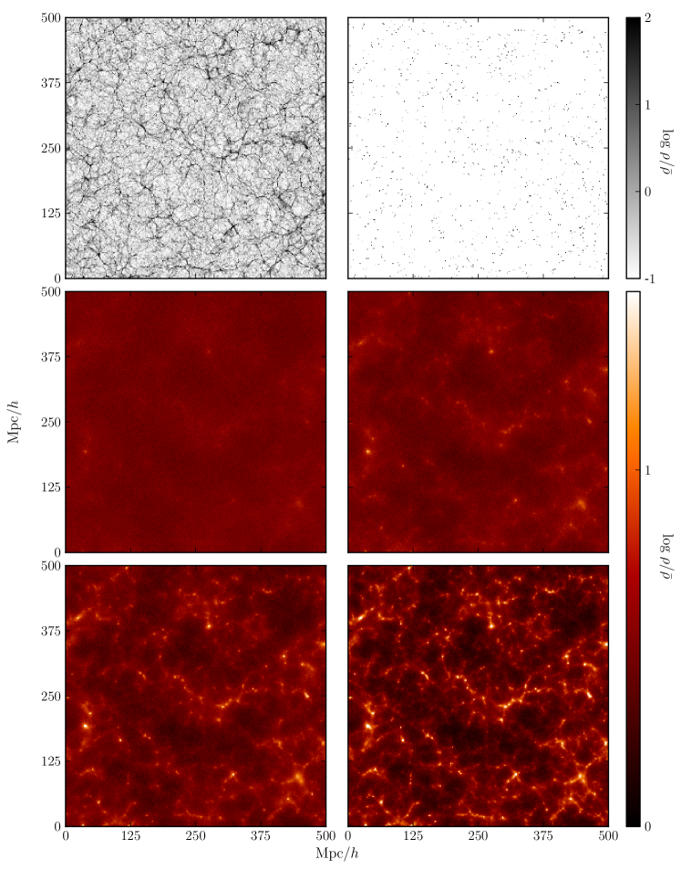
Figure 1: Density slices of equal width $500\ \mbox{Mpc}/\mbox{h}{}$ and thickness $1.3\ \mbox{Mpc}/\mbox{h}{}$ from various simulations at $z=0$. The top row shows dark matter (left) and halo (right) density slices from the 0.2 eV neutrino simulation. The middle row compares neutrino density slices from the 0.05 (left) and 0.1 (right) eV simulations while the bottom row shows the 0.2 (left) and 0.4 (right) eV simulations. It is easy to see by eye that the dark matter and neutrino density fields are highly correlated and that heavier neutrinos cluster more than lighter ones.

Fig. 1 compares slices of the dark matter and halo density fields at $z=0$ from simulation S2 to the neutrino density fields from simulations S05, S1, S2, and S4. It is easy to see that the neutrino density fields are correlated with the dark matter density field albeit with much less clumping in the former than the latter as evidenced by their respective colour bars. In addition, we see that higher mass neutrinos tend to clump more than lower mass neutrinos as they are more influenced by the underlying dark matter distribution due to their lower thermal velocities.

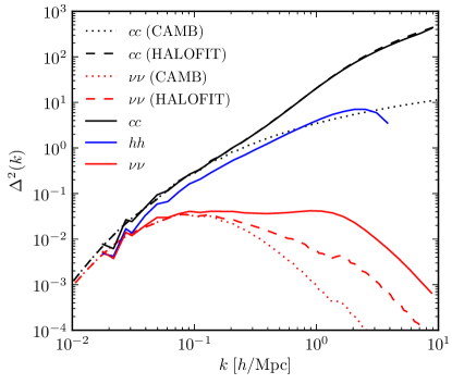
Figure 2: The dimensionless matter power spectra at $z=0$ for dark matter (solid black line), halos (solid blue line) and neutrinos (solid red line) from S2. Shot noise has been removed by computing the cross-spectrum between two randomly chosen groups for each species. Also plotted are the linear and non-linear dark matter (dotted black and dashed black lines) and neutrino (dotted red and dashed red lines) power spectra. Note that there is a small numerical artifact in the linear neutrino transfer function just above $k=1\>\mbox{h}/\mbox{Mpc}$ that should be ignored.

Fig. 2 shows the dimensionless power spectra for dark matter, halos, and neutrinos at $z=0$ from S2. Also plotted are theoretical predictions for dark matter and neutrinos, which are computed via

$$\Delta^{2}_{i}(k)=\frac{k^{3}}{2\pi^{2}}P_{m}\left(\frac{T_{i}}{T_{m}}\right)^{2},$$ (11)

where $T_{i}$ is the linear transfer function for species $i$, $T_{m}$ is the total matter linear transfer function, and $P_{m}$ is either the linear (computed from CAMB) or the non-linear (computed from HALOFIT) total matter power spectrum. We first note that the group cross-correlation method we employ effectively removes the shot noise allowing us to understand statistical properties even of the noisy neutrino density field. We find that the dark matter power spectrum agrees well with the non-linear prediction up to large $k$. The neutrino power spectrum, on the other hand, is significantly enhanced on small scales compared to the theoretical curve. This trend was previously observed by (Ali-Haïmoud, ) and is yet to be understood.

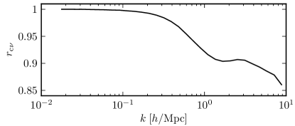
Figure 3: The dark matter-neutrino cross correlation coefficient at $z=0$ from S2. As expected, neutrinos are highly correlated with dark matter over a large range of scales.

Despite their enhanced power on small scales, neutrinos remain highly correlated with the dark matter density field, as was qualitatively discussed with Fig. 2. More quantitatively, Fig. 3 shows the $z=0$ cross-correlation coefficient between dark matter and neutrinos from S2 as a function of wavenumber. We find that neutrinos exhibit $r_{c\nu}\gtrsim.90$ correlation with dark matter on all scales $k<1\ \mbox{h}/\mbox{Mpc}$ and achieve $r_{c\nu}\sim.85$ down to the smallest scales resolved in the simulation.

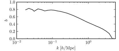
Figure 4: The halo bias parameter measured from S2 at $z=0$. On scales $k\lesssim 0.2\ h/{\rm Mpc}$ the bias is roughly constant with $b\sim 0.8$. The bias falls off on smaller scales as power is suppressed within the typical virial radii of halos.

The halo power spectrum is also plotted in Fig. 2. As expected, the halo power follows the general shape of the dark matter power spectrum, but with a reduced amplitude, or bias. This bias is defined as:

$$b\equiv\sqrt{\frac{P_{hh}}{P_{cc}}},$$ (12)

and is plotted as a function of $k$ in Fig. 4. The bias is roughly constant on large scales with $b\sim 0.8$ and falls off on small scales as the halo density field does not include contributions from the “one-halo” term describing the internal mass profile of halos (Scherrer and Bertschinger, 1991). Hence, halo power is suppressed on scales comparable to the typical virial radii of halos which occurs at $k\sim 0.2\ h/{\rm Mpc}$ for the largest halos in the box.

III.2 Velocity

Fig. 5 compares slices of dark matter, neutrino, and dark matter-neutrino relative velocity computed from the simulation particles as well as reconstructed from the dark matter and halo density fields using Eq. 6. We observe a similar trend as the density fields with dark matter and neutrinos highly correlated in velocity. In addition, we see that the velocity fields reconstructed from only knowledge of either the dark matter or halo density field qualitatively agree with the large-scale structure of the velocity fields obtained within the simulation.

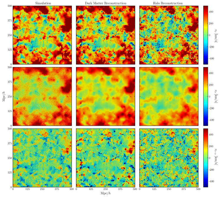
Figure 5: Slices of equal width $500\ \mbox{Mpc}/\mbox{h}{}$ and thickness $1.3\ \mbox{Mpc}/\mbox{h}{}$ showing the $z=0$ velocity component perpendicular to the page for dark matter (top row), neutrinos (middle row), and the relative velocity between dark matter and neutrinos (bottom row). Columns show the velocity fields from the simulation particles (left column), reconstructed from the dark matter density field (middle column), and reconstructed from the halo density field (right column). We see that both of the reconstruction methods agree well with the large-scale structure of the simulation velocity fields.

Fig. 6 compares the simulated dark matter and neutrino velocity power spectra to the dark matter and halo reconstructed fields. Note that for the latter we take $\delta=\delta_{h}/b$ in Eq. 6 to account for the halo bias. We use a value of $b=0.80$ consistent with the large-scale bias found in Fig. 4. We compute theoretical predictions for the velocity power using Eq. 11 with $T_{i}$ being a velocity transfer function. We note that the groups method has also effectively removed shot noise from the velocity power just as for the density.

Fig. 6 demonstrates that the simulated dark matter velocity field is suppressed on scales $0.2\lesssim k\lesssim 4.0\>\mbox{h}/\mbox{Mpc}{}$ compared to the linear and non-linear expectations. This suppression was also seen in (Pueblas and Scoccimarro, 2009; Hahn et al., 2014) and may be due to the thermalization of dark matter within collapsed objects. The velocity field reconstructed from dark matter agrees well with the non-linear expectation of Eq. 11. This is simply a reflection of the agreement between the dark matter density field and HALOFIT shown in Fig. 2. If we used the full bias curve, $b(k)$, instead of a constant then the halo reconstruction method works equally well. Neutrinos, on the other hand, have a velocity power spectrum that agrees well with the non-linear expectation on scales $k\lesssim 0.15\>\mbox{h}/\mbox{Mpc}$. However, we find that they are underpredicted by linear theory on small scales. It is unclear why neutrinos behave in an opposite manner from dark matter.

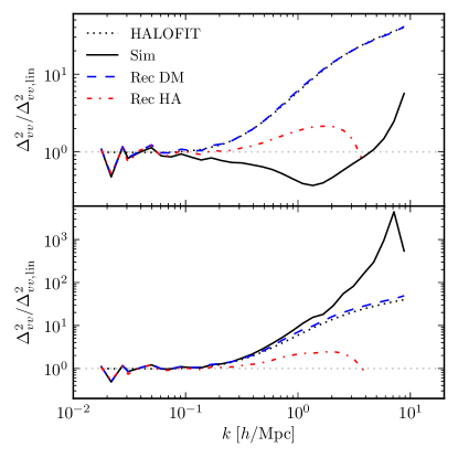
Figure 6: Velocity power spectra at $z=0$ from S2 for dark matter (top) and neutrinos (bottom) normalized to the linear theory result obtained from Eq. 11. In each panel, the dotted black line shows the non-linear expectation of Eq. 11, the solid black line shows the simulation result, and the dashed blue line (dot-dashed red line) shows the velocity field reconstructed from Eq. 6 using the dark matter (halo) density field.

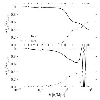
Figure 7: Relative fraction of the divergence (solid black line) and curl (dotted black line) components of the dark matter (top) and neutrino (bottom) velocity power at $z=0$ from S2. In each case, the curl component is negligible on scales $k\lesssim 1\ \mbox{h}/\mbox{Mpc}{}$. The oscillations seen with the neutrino power on small scales is indicative of their shot noise.

The efficacy of reconstructing velocities using Eq. 6 relies on the linearity of the velocity field. To test this we decompose velocity into divergence and curl components. We have performed this computation using both real-space finite differencing of the velocity field as well as Fourier space decomposition:

$$\vec{v}_{k} =\hat{k}(\hat{k}\cdot\vec{v}_{k})+\hat{k}\times(\hat{k}\times\vec{v}_{k})$$ (13)

$$=\hat{k}D+\vec{C},$$

where $D$ is the divergence field and $\vec{C}=\vec{v}_{k}-\hat{k}D$ is the curl field. Both the real-space and Fourier-space methods produce equivalent results. In linear theory, the velocity is parallel to $\hat{k}$ and therefore has no curl. Hence, the presence of a curl component of the velocity field allows us to measure its degree of non-linearity.

In Fig. 7 we plot the divergence and curl components of both the dark matter and neutrino velocity fields. In each case, we see that the velocity is curl-free on scales $k\lesssim 1\ \mbox{h}/\mbox{Mpc}{}$. The only significant curl component occurs for dark matter on scales $k\gtrsim 5\ \mbox{h}/\mbox{Mpc}{}$. This result highlights that the discrepancy between the simulated dark matter velocity and theoretical curves in Fig. 6 is not due to the presence of a curl component but rather due to non-linear processes affecting the divergence.

III.3 Relative Velocity

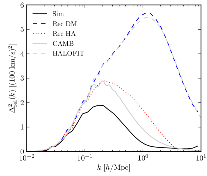
Figure 8: The dark matter-neutrino relative velocity power spectrum at $z=0$ for S2 (black line) compared to the dark matter (dashed blue) and halo (dotted red) reconstructed fields as well as the linear (solid gray) and non-linear (dashed gray) predictions. The simulated relative velocity power is similar to the linear prediction whereas the two reconstructed fields deviate from the linear curve due to non-linear structure formation.

Fig. 8 compares the dark matter-neutrino relative velocity power spectrum to linear and non-linear predictions as well as to the two reconstruction methods. The relative velocity field from the simulations is roughly similar to the linear theory expectation, being within a factor of $3$ on scales $k<5\>\mbox{h}/\mbox{Mpc}$. The power spectra from the halo reconstruction method is also similar to the linear theory result. The field reconstructed from dark matter looks very different from the previous two but is consistent with the non-linear expectation. This can be made consistent with the linear theory result by simply multiplying Eq. 6 by the ratio between the linear and non-linear dark matter density power spectra.

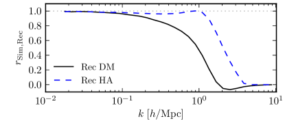
Figure 9: The dark matter-neutrino relative velocity correlation coefficient between the simulated field and the field reconstructed from dark matter (solid black line) and halo (dashed blue line) density fields. Both methods are highly correlated over all relevant scales.

Fig. 9 shows the correlation coefficient defined in Eq. 8 between the simulated and reconstructed relative velocity fields. We see that both reconstruction methods reproduce the relative velocity field well over the scales of interest. In particular, the halo reconstruction achieves nearly perfect correlation on scales $k\lesssim 1\ \mbox{h}/\mbox{Mpc}{}$. The velocity correlation coefficient is a measure of how well the vector fields agree in direction as the denominator in Eq. 8 divides out the magnitudes. Thus, Fig. 9 demonstrates that we are able to reconstruct the direction of the relative velocity field accurately.

Fig. 10 shows the relative velocity power spectra for each of the four neutrino masses using the nearest particle/momentum method. We find that they follow the same trends: lighter neutrinos have less relative velocity and the linear prediction is larger than in simulation. Table 1 lists the integrated correlation coefficients as a function of neutrino mass between simulated and halo reconstructed velocities for dark matter, neutrino and dark matter-neutrino relative velocities. We find that there is a large correlation between these methods indicating that the reconstruction method is accurately reproducing the simulation velocities.

Table 1: The integrated correlation coefficient defined in Eq. 9 between the simulated velocities and those reconstructed by halos for dark matter, neutrinos and dark matter-neutrino relative velocities.

$m_{\nu}$	Dark Matter	Neutrinos	Relative
0.05	0.95	0.98	0.94
0.1	0.95	0.97	0.93
0.2	0.95	0.97	0.91
0.4	0.95	0.97	0.88

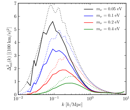
Figure 10: The dark matter-neutrino relative velocity power spectra via the nearest particle/momentum method for all four neutrino masses (solid) along with theoretical predictions (dashed). The power is clearly suppressed compared to linear theory but behaves qualitatively similar with varying masses.

Finally, in Fig. 11 we show the relative velocity correlation lengths, $\xi_{1/2}$, defined as in (Zhu et al., 2014a) to be the point at which the relative velocity correlation function,

$$\xi_{\nu c}(r)=\int\frac{dk}{k}\Delta^{2}_{\nu c}\frac{\sin(kr)}{kr}$$ (14)

reaches half its maximum value. This scale can be thought of as the size of a region with a uniform velocity field. Lighter neutrinos are less affected by large scale structure due to their larger thermal velocities and so are coherent over larger regions. Fig. 11 shows these correlation lengths as a function of neutrino mass. We find that the simulations exhibit a slightly larger correlation length for each neutrino mass compared to the theoretical predictions. The shapes of the curves remain similar, however, with both having power law slope which we fit to have an exponent $-0.44$.

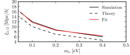
Figure 11: The correlation length defined to be the distance for which the correlation function in Eq. 14 drops to half its maximum value for varying neutrino masses. The simulations have longer correlation lengths but follow a similar power law behaviour.

IV Discussion

We have tested four methods of computing the velocity field: a nearest particle method, a momentum method, and reconstruction via dark matter and halo density fields. Our results are generally consistent with theoretical expectations and highly correlated among each other. Specifically we have demonstrated that reconstructing the velocity from point-particle halos produces a velocity field highly correlated with that of our N-body particles. It is the near unit correlation coefficient - a measure of the angle between the two fields - that ensures that the reconstructed velocity points in the right direction. The magnitude of the velocity can then simply be scaled to the correct value as long as the bias is known.

This result allows for a prescription to determine the actual velocity fields in our own Universe.

1. Reconstruct the galaxy density field from a galaxy survey catalogue. We expect this reconstruction to be very comparable to the halo reconstruction we use here except with the addition of a 1-halo term to make the bias constant over more wavenumbers.

2. Fourier transform the gridded density field. Then, use Eq. 6 to compute the dark matter, neutrino and relative velocity fields in Fourier space. Here, a non-linear correction can be applied by additionally multiplying by a factor of $\Delta_{v}^{\rm Sim}/\Delta_{v}^{\rm RecHA}$.

3. Fourier transform back to real space.

We first note that a similar process could be performed on the density fields produced by 21 cm observations. We also note that redshift distortions and masking effects might result in extra biases in the reconstruction scheme. We intend to investigate these effects in a future paper.

Our results also provide support for the applicability of the analysis performed in (Zhu et al., 2014a, b). They used moving background perturbation theory to study the neutrino relative velocity effect. The moving background approximation relies on having a coherent background relative flow and our simulation results indicate that the coherency scales of such motions are larger than predicted. Thus, we expect that inaccuracies in the predicted dipole distortion to the correlation function will come from non-linear evolution rather than the moving background approximation. We note that we can also directly measure the dipole correlation function in our simulations and plan to report on this in a subsequent paper.

V Conclusion

We performed a set of four large N-body simulations including cold dark matter and neutrinos of varying mass. We have accurately measured the dark matter-neutrino relative velocity. We find that we can accurately reconstruct this velocity using a linear theory approach and halo density fields. We have described a simple method for accurately predicting the relative velocity field via a galaxy survey or 21 cm observations. Since such a reconstruction allows for an independent measurement of neutrino masses, we expect this technique to provide significant constraints in upcoming astronomical surveys.

VI Acknowledgements

We acknowledge valuable discussions with Joel Meyers and Yu Yu. We acknowledge the support of NSERC.

Computations were performed on the GPC supercomputer at the SciNet HPC Consortium (Loken et al., 2010). SciNet is funded by: the Canada Foundation for Innovation under the auspices of Compute Canada; the Government of Ontario; Ontario Research Fund - Research Excellence; and the University of Toronto.

References

- Fogli et al. (2012) G. L. Fogli, E. Lisi, A. Marrone, D. Montanino, A. Palazzo, and A. M. Rotunno, Phys. Rev. D 86, 013012 (2012), eprint 1205.5254.
- Planck Collaboration et al. (2015) Planck Collaboration, P. A. R. Ade, N. Aghanim, M. Arnaud, M. Ashdown, J. Aumont, C. Baccigalupi, A. J. Banday, R. B. Barreiro, J. G. Bartlett, et al., ArXiv e-prints (2015), eprint 1502.01589.
- Zhu et al. (2014a) H.-M. Zhu, U.-L. Pen, X. Chen, D. Inman, and Y. Yu, Physical Review Letters 113, 131301 (2014a), eprint 1311.3422.
- Zhu et al. (2014b) H.-M. Zhu, U.-L. Pen, X. Chen, and D. Inman, ArXiv e-prints (2014b), eprint 1412.1660.
- Brandbyge and Hannestad (2009) J. Brandbyge and S. Hannestad, J. Cosmology Astropart. Phys 5, 002 (2009), eprint 0812.3149.
- Brandbyge and Hannestad (2010) J. Brandbyge and S. Hannestad, J. Cosmology Astropart. Phys 1, 021 (2010), eprint 0908.1969.
- Bird et al. (2012) S. Bird, M. Viel, and M. G. Haehnelt, MNRAS 420, 2551 (2012), eprint 1109.4416.
- Ali-Haïmoud and Bird (2013) Y. Ali-Haïmoud and S. Bird, MNRAS 428, 3375 (2013), eprint 1209.0461.
- Harnois-Déraps et al. (2013) J. Harnois-Déraps, U.-L. Pen, I. T. Iliev, H. Merz, J. D. Emberson, and V. Desjacques, MNRAS 436, 540 (2013), eprint 1208.5098.
- Lewis et al. (2000) A. Lewis, A. Challinor, and A. Lasenby, The Astrophysical Journal 538, 473 (2000).
- Blas et al. (2011) D. Blas, J. Lesgourgues, and T. Tram, Journal of Cosmology and Astroparticle Physics 2011, 034 (2011).
- Zhang et al. (2014) P. Zhang, Y. Zheng, and Y. Jing, ArXiv e-prints (2014), eprint 1405.7125.
- Zheng et al. (2014) Y. Zheng, P. Zhang, and Y. Jing, ArXiv e-prints (2014), eprint 1409.6809.
- Pueblas and Scoccimarro (2009) S. Pueblas and R. Scoccimarro, Phys. Rev. D 80, 043504 (2009), URL http://link.aps.org/doi/10.1103/PhysRevD.80.043504.
- Hahn et al. (2014) O. Hahn, R. E. Angulo, and T. Abel, ArXiv e-prints (2014), eprint 1404.2280.
- Mangano et al. (2005) G. Mangano, G. Miele, S. Pastor, T. Pinto, O. Pisanti, and P. D. Serpico, Nuclear Physics B 729, 221 (2005), eprint hep-ph/0506164.
- (17) Y. Ali-Haïmoud, Private communication.
- Scherrer and Bertschinger (1991) R. J. Scherrer and E. Bertschinger, ApJ 381, 349 (1991).
- Loken et al. (2010) C. Loken, D. Gruner, L. Groer, R. Peltier, N. Bunn, M. Craig, T. Henriques, J. Dempsey, C.-H. Yu, J. Chen, et al., Journal of Physics: Conference Series 256, 012026 (2010), URL http://stacks.iop.org/1742-6596/256/i=1/a=012026.