Differential Neutrino Condensation onto Cosmic Structure

Abstract

Astrophysical techniques have pioneered the discovery of neutrino mass properties. Current cosmological observations give an upper bound on neutrino masses by attempting to disentangle the small neutrino contribution from the sum of all matter using precise theoretical models. We discover the differential neutrino condensation effect in our TianNu $N$-body simulation. Neutrino masses can be inferred using this effect by comparing galaxy properties in regions of the universe with different neutrino relative abundance (i.e. the local neutrino to cold dark matter density ratio). In “neutrino-rich” regions, more neutrinos can be captured by massive halos compared to “neutrino-poor” regions. This effect differentially skews the halo mass function and opens up the path to independent neutrino mass measurements in current or future galaxy surveys.

Department of Astronomy, Beijing Normal University, Beijing 100875, China

Kavli Institute for Astronomy & Astrophysics, Peking University, Beijing 100871, China

Canadian Institute for Theoretical Astrophysics, University of Toronto, M5S 3H8, Ontario, Canada

Department of Astronomy & Astrophysics, University of Toronto, Toronto, Ontario M5S 3H4, Canada

Department of Physics, University of Toronto, Toronto, Ontario M5S 1A7, Canada

Shandong Provincial Key Laboratory of Biophysics, School of Physics and Electric Information, Dezhou University, Dezhou 253023, China

Dunlap Institute for Astronomy and Astrophysics, University of Toronto, Toronto, ON M5S 3H4, Canada

Canadian Institute for Advanced Research, Program in Cosmology and Gravitation

Perimeter Institute for Theoretical Physics, Waterloo, ON, N2L 2Y5, Canada

Department of Physics & Astronomy, University of British Columbia, Vancouver, B.C. V6T 1Z1, Canada

Scottish University Physics Alliance, Institute for Astronomy, University of Edinburgh, EH9 3HJ, Scotland, UK

Department of Astronomy, Peking University, Beijing 100871, China

Key Laboratory for Computational Astrophysics, National Astronomical Observatories, Chinese Academy of Sciences, Beijing 100012, China

School of Physical Sciences, University of Chinese Academy of Sciences, Beijing 100049, China

Institute of High Energy Physics, Chinese Academy of Sciences, Beijing 100049, China

School of Computer, National University of Defense Technology, Changsha 410073, China

National Supercomputer Center in Guangzhou, Sun Yat-Sen University

Institute of Ocean Science and Technology, National University of Defense Technology

Neutrinos are elusive elementary particles whose fundamental properties are incredibly difficult to measure. 40 years after their first direct detection [1, 2], flavour oscillation experiments [3, 4, 5] confirmed that at least two neutrino types are massive and placed a lower bound on the sum of their mass: $M_{\nu}\equiv\sum_{i=1}^{3}m_{\nu_{i}}\gtrsim$ 0.05 eV [6]. This discovery has a profound impact on our understanding of the early Universe, where neutrinos are produced in great numbers. First in a relativistic state, they contribute to the radiation energy density, thereby modulating the matter-to-radiation ratio in a way that depends on their mass. This leaves an imprint on the Cosmic Microwave Background (CMB) that can be searched for, providing a current upper bound of $M_{\nu}\lesssim$ 0.23 eV [7]. As the Universe expands, the neutrinos lose momentum and eventually become non-relativistic, at which point they contribute instead to the matter energy density. Although small, this neutrino component has consequences on the clustering properties of matter, which can be measured in observations of the Large Scale Structure (LSS). Despite having a current temperature of roughly 2 K today, these relic neutrinos maintain a velocity dispersion that is significantly higher than both baryons and cold dark matter (CDM). This thermal motion (free streaming) reduces their susceptibility to gravitational capture, leading to suppressions in the matter power spectrum. Upcoming cosmological missions that probe the large-scale structure of the Universe, such as Euclid [8], LSST [9], eBOSS [10], and DESI [11], will complement CMB measurements and are expected to improve this upper bound in the near future [12]. Unfortunately, it is extremely difficult to disentangle this suppression from differences in modelling of the non-linear gravitational growth and galaxy/halo bias, the uncertain impact of baryonic processes and potentially alternate models of gravity [13].

While there have been some attempts to study the interplay between neutrinos and LSS analytically [14], the current understanding of their non-linear dynamics heavily relies on cosmological $N$-body simulations that coevolve both CDM and neutrino particles (e.g. [15]). These allow to investigations of, for example, the effects of massive neutrinos on the halo mass function and on the galaxy bias, or to study the neutrino density profile [16, 17, 18]. The precision of these subtle measurements is limited both by the simulation volumes and Poisson noise, and is challenging even for modern high performance computing centres.

Taking advantage of a development phase of the Tianhe-2 supercomputer, we have completed the world’s largest cosmological $N$-body simulation, named “TianNu”, which coevolved just under 3 trillion CDM and neutrino particles. From this calculation we find that regions with same CDM density can have substantially different mean neutrino densities due to the free streaming of neutrinos. Consequentially, collapsed dark matter halos that live in “neutrino-rich” sectors of the Universe have deeper gravitational potential wells to trap even more CDM and baryons, compared to otherwise identical halos from “neutrino-poor” regions. This is a novel form of feedback on the cosmic structure whose strength depends on $M_{\nu}$, which we refer to as differential neutrino condensation. It results in spatial variations of halo properties that depend on the difference between the neutrinos and CDM rather than on their sum, and as such provides a clean probe of $M_{\nu}$ than conventional LSS probes.

(Simulation.)

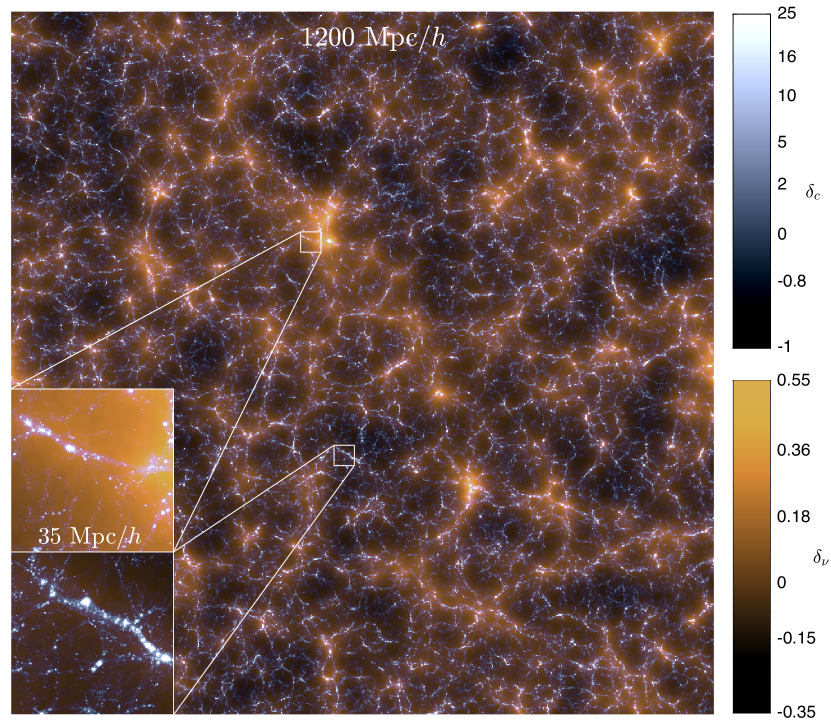
Figure 1: TianNu simulation. Two-dimensional visualisation of CDM and neutrino structures in TianNu. CDM is represented in blue-white and neutrinos in orange. The two subpanels focus on regions with similar CDM structure but different neutrino-to-CDM density ratios. The upper panel shows a neutrino-rich region with $(\delta_{c},\delta_{\nu})=(0.081,0.19)$ while the lower panel shows a neutrino-poor region for which $(\delta_{c},\delta_{\nu})=(0.44,-0.047)$. Density contrasts are averaged over the volume of each subpanel, $35^{2}\times 8.3\ ({\rm Mpc}/h)^{3}$. The difference in neutrino condensation seen in these two panels leads to systematically different halo properties between the two regions.

TianNu was carried out with a modified version of the public cosmological $N$-body code cubep³m [19] that includes CDM and neutrino coevolution [20]. The neutrino sector in TianNu models the minimal “normal hierarchy” of the neutrinos, in which 2.046 massless neutrino species are included in the background cosmology at the level of the initial transfer function [21], and one $m_{\nu}=0.05$ eV neutrino species is explicitly traced using $N$-body particles. The background cosmological environment is otherwise described by the densities of CDM and baryons, Hubble’s parameter, the initial tilt and fluctuations of the power spectrum, which are parameterised with [$\Omega_{c},\Omega_{b},h,n_{s},\sigma_{8}$] = [0.27, 0.05, 0.67, 0.96, 0.83]. We finally impose flatness by setting $\Omega_{\Lambda}=1-\Omega_{m}$, where the total matter density is $\Omega_{m}=\Omega_{b}+\Omega_{c}+\Omega_{\nu}$. $6912^{3}$ CDM and $13824^{3}$ neutrino $N$-body particles are coevolved in a cosmological volume of $L=1.2$ ${\rm Gpc}/h$ on the side. which is comparable to a shallower, lower redshift galaxy survey, in which neutrino effects are relatively prominent. For comparison and calibration purposes, we ran a neutrino-free simulation (equivalent to a TianNu simulation in which all $m_{\nu}=0$ eV) with same initial condition and $\Omega_{m}$ fixed, named “TianZero”.

Fig.1 shows a two-dimensional projection of a thin slice of thickness $8.3$ ${\rm Mpc}/h$ extracted from the TianNu simulation at $z=0.01$. The blue-white colour scale shows the CDM component $\delta_{c}$, while orange highlights the neutrinos, $\delta_{\nu}$. Here $\delta_{i}$ are the density contrasts obtained from the density fields $\rho$ with $\delta_{i}\equiv\rho_{i}/\bar{\rho_{i}}-1$. $\delta_{c}$ exhibits the “cosmic web” structure, mostly arranged into filaments and collapsed halos. On scales $k^{-1}>100$ ${\rm Mpc}/h$, which is much larger than neutrino’s free streaming scale, $\delta_{c}$ and $\delta_{\nu}$ are coupled via their mutual gravitational potential and have similar structures. However, due to the free streaming, on smaller scales $k^{-1}<20$ ${\rm Mpc}/h$, neutrinos are instead distributed as diffuse “condensation clouds” centered on the largest CDM structures and so $\delta_{\nu}$ is less correlated with $\delta_{c}$. We find that, this environmental difference between $\delta_{c}$ and $\delta_{\nu}$ on the scale $k^{-1}\simeq 10$ ${\rm Mpc}/h$, causes systematic modulations on CDM halo (of scale $k^{-1}\simeq 2$ ${\rm Mpc}/h$) properties. The two subpanels in Fig.1 provide a visual representation of the large variations in the local difference of $\delta_{c}$ and $\delta_{\nu}$ in regions with otherwise similar LSS.

(Halo masses.)

In order to demonstrate how the properties of galaxies are affected by differences in their neutrino environment, we first search for collapsed structures in both TianNu and TianZero. We identify spherical CDM halos, which are the regions that host galaxies. For each halo, we record the total mass $m_{h}$ and position $\vec{x}$, rejecting under-resolved halos with mass $m_{h}<3.5\times 10^{11}~{}M_{\odot}$. We do not include neutrinos in the evaluation of $m$ since the observable quantity that we measure – the luminosity of its constituent galaxies – correlates only with the CDM mass. Since both simulations have the exact same CDM initial conditions, systematic differences in their halo properties are caused by the neutrino mass. The first step in this comparison consists in matching halos in TianZero with their counterpart in TianNu, representing the evolution of the same physical object in different cosmologies. Then we sort all halos in descending order according to their masses, and assign a rank, $r$, to each halo, defined as its index in the sorted list. This mass rank serves as a proxy for observational properties of galaxies (e.g. by abundance matching [22, 23, 24], halo occupation distribution [25, 26]). The ranks $r_{\nu}$ and $r_{0}$ obtained from TianNu and TianZero are in general different, which means that the presence of massive neutrinos affects the final mass of collapsed structures in a way that depends not only on the halo mass – the rank would be unchanged – but also on their environment.

We next estimate the forementioned local values of $\delta_{c}$ and $\delta_{\nu}$ centered on the position of each halo, by a reconstruction technique [20] that estimates the CDM and neutrino density fields directly from the halo catalogues. The resulting quantities, $\hat{\delta}_{c}$ and $\hat{\delta}_{\nu}$, on scale $k^{-1}\simeq 10$ ${\rm Mpc}/h$, describe the two environment variables that are responsible for the changes of halo ranks between TianNu and TianZero. These can be extracted from galaxy redshift surveys, thereby leading to a measurable neutrino effect. Neutrino mass has effect primarily on halo masses rather than halo positions, so halo catalogue from either TianNu and TianZero gives same estimation of $\hat{\delta}_{c}$ and $\hat{\delta}_{\nu}$. We examined that the results are insensitive to the reconstruction accuracy.

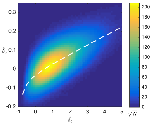
Figure 2: Distribution of dark matter halos as a function of environmental variables $\hat{\delta}_{c}$ and $\hat{\delta}_{\nu}$. This figure exhibits the correlation between the two quantities, and the considerable amount of spread. The dashed line shows the mean value of $\hat{\delta}_{\nu}$ in each $\hat{\delta}_{c}$ bin, which serves as a baseline to define the “neutrino excess” $\epsilon_{\nu}$.

In Fig.2 we plot the $\hat{\delta}_{c}$ and $\hat{\delta}_{\nu}$’s distribution of halos. The correlation between the two quantities (with a Pearson’s $r$ $\rho_{c,\nu}=0.663$) shows their coupling above neutrino’s free streaming scale. Namely, regions of high (low) $\hat{\delta}_{c}$ have generally high (low) $\hat{\delta}_{\nu}$. This correlation is undesired, as any observable dependence on $\hat{\delta}_{\nu}$ is entangled with $\hat{\delta}_{c}$. However, the considerable amount of spread in Fig.2 indicates that halos residing in identical $\hat{\delta}_{c}$ regions need not have same $\hat{\delta}_{\nu}$ environments. In order to disentangle the net neutrino’s contribution from CDM’s contribution, we subtract the mean correlation and consider only the scatter of $\hat{\delta}_{\nu}$ at a given $\hat{\delta}_{c}$, i.e., for a given $\hat{\delta}_{c}$, we measure the expectation values of $\hat{\delta}_{\nu}$, $\langle\hat{\delta_{\nu}}\rangle$, indicated with the dashed line in the figure. From this quantity we define the “neutrino excess”, $\epsilon_{\nu}\equiv\hat{\delta_{\nu}}-\langle\hat{\delta}_{\nu}\rangle$, which is uncorrelated with $\delta_{c}$. A halo with $\epsilon_{\nu}>0$ is located in a region with relatively high neutrino density; and we refer it to “neutrino-rich” region. On the contrary, $\epsilon_{\nu}<0$ refers to “neutrino-poor” regions. This is a quantitative measure of difference of the CDM and neutrino abundance caused by differential neutrino condensation.

The dominant effect of this differential condensation is to alter the rank ordering of halos. To illustrate this, we measure the relative variation of rank between the TianNu and TianZero simulations, $\Delta r/r\equiv(r_{\nu}-r_{0})/r_{0}$, measured from each halo pair, and organise the results as a function of neutrino excess and rank. This is shown in Fig.3, where the colour scale indicates the expectation value of the relative change in rank as a function of rank and $\epsilon_{\nu}$. We rescale each pixel by a weight function $w=\sqrt{N}$, where $N$ is the number of halos in each pixel. The top axis provides a conversion from rank to halo mass. We can see that the neutrino-rich (upper part) regions are bluer, meaning that the mass of halos in TianNu tend to be systematically increased (the rank decreases) by the presence of high neutrino condensation compared to the TianZero baseline. Similarly, while the neutrino poor (bottom part) regions are redder, corresponding to a systematic decrease of the halo mass in neutrino-poor regions. This is a manifestation of “differential neutrino condensation”, and its impact on cosmic structure is the strongest for cluster-scale halos ($m_{h}\gtrsim 10^{13}M_{\odot}$). It is a characteristic signature of the gravitational feedback of modulations in the neutrino density onto the growth of CDM halos.

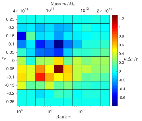
Figure 3: Relative variation in halo mass and rank caused by differential neutrino condensation. The colour scale shows a weighted histogram of the relative rank variations observed between TianNu and TianZero, $\Delta r/r\equiv(r_{\nu}-r_{0})/r_{0}$, organized in bins of halo rank (or mass) and neutrino excess $\epsilon_{\nu}$. More massive halos (lower rank) that live in neutrino-rich regions condense enough neutrinos to lower their ranks and increase their mass. Conversely, in neutrino-poor regions, equally large halos lose mass due to neutrino free streaming, increasing their rank. This effect becomes weaker for less massive halos since these are less efficient in condensing neutrinos.

The global trends in rank variations can be expressed by a linear function of $r$ and $\epsilon_{\nu}$. The rank is first held fixed, and the variations in $\Delta r/r$ with changing $\epsilon_{\nu}$ (e.g. columns in Fig. 3) are fit with a straight line. The slope of this line, $\partial(\Delta r/r)/\partial\hat{\delta}_{\nu}$, is shown in Fig.4 for different rank bins. We repeat this measurement from 1000 bootstrap resamplings of the halo catalogues in order to estimate the error bars. These points are all negative, indicating that for a halo of rank $r$, a net increase of neutrino density $\partial\hat{\delta}_{\nu}$ lowers the rank by $\partial(\Delta r/r)$. The effect asymptotes to zero as the halo mass decreases, reflecting the results seen in the rightmost region of Fig.3. On the high-mass end, the measurements are well described by $\partial(\Delta r/r)/\partial\hat{\delta}_{\nu}=\alpha\log_{10}(r/r_{\rm pivot})+\beta$, with $\{\alpha,\beta\}=\{0.00254\pm 0.00073,-0.00194\pm 0.00017\}$, shown as the red dashed line in Fig.4. The value $r_{\rm pivot}=8.1\times 10^{5}$ is chosen such that $\alpha$ and $\beta$ are uncorrelated.

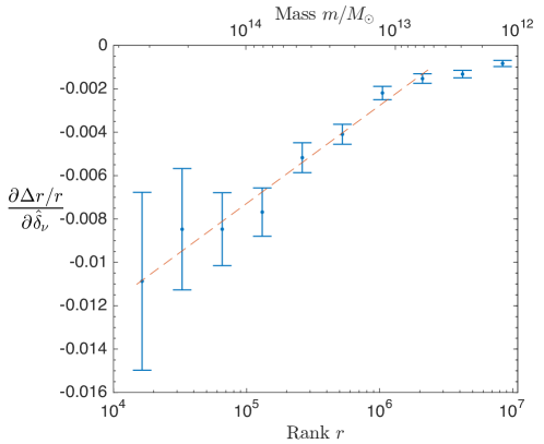
Figure 4: Differential modulation in halo rank caused by neutrino condensation. The measurements are shown as a function of halo mass (and rank), and the error bars are from bootstrap resampling. All points are negative with strong signal to noise, indicating that differential neutrino condensation has an impact on all halos. The effect is stronger for high mass halos (low rank) since they can trigger neutrino condensation in a more effective way, provided they are in a region of high $\epsilon_{\nu}$. The red dashed line represents the best linear fit to the measurement, for mass $m>5\times 10^{12}M_{\odot}$.

(Discussion and conclusion.)

The TianNu and TianZero simulation demonstrate a controlled numerical experiment to show the differential neutrino condensation effect. In order to isolate neutrino effects while cancelling CDM and baryon contributions to halo properties, we perform three differences. First, we use neutrino excess $\epsilon_{\nu}$, a quantity uncorrelated with CDM density, to distinguish regions in our simulation that are neutrino-rich and neutrino-poor, according to the local (on scale $k^{-1}\simeq 10$ ${\rm Mpc}/h$) difference between $\delta_{c}$ and $\delta_{\nu}$. Second, we search for halos’ mass/rank differences between TianNu ($M_{\nu}=0.05$ eV) and TianZero ($M_{\nu}=0$ eV), and find their dependence on the neutrino excess $\epsilon_{\nu}$. This dependence, written in $\partial(\Delta r/r)/\partial\hat{\delta}_{\nu}$ relies on the net change of neutrinos density, and is cleanly separated from $\delta_{c}$-$\delta_{\nu}$’s correlation and potential baryonic effects. Finally, we investigate how this dependence changes with halo mass and find that the mass/rank of heavier halos are more significantly affected by a net change of neutrino density. The next step is to determine how this can be robustly measured in astronomical observations. The analysis in this report focussed on plausibly observable quantities, specifically neutrino and dark matter densities $\hat{\delta}_{c}$ and $\hat{\delta}_{\nu}$ reconstructed from halo catalogs fields, and rank order $r$ as proxy for luminosity or number count observables. The clean separation of cosmological regions into neutrino poor and rich needs to be carefully controlled to cancel generic dark matter contributions or potential super-sample variance [27] to halo properties.

Methods and numerical details are available in the supplemental material.

References

The TianNu and TianZero simulations were performed on Tianhe-2 supercomputer at the National Super Computing Centre in Guangzhou. The analysis were performed on the GPC and BGQ supercomputer at the SciNet HPC Consortium. This work was supported by the National Science Foundation of China (Grants No. 11573006, 11528306, 10473002, 11135009), the Ministry of Science and Technology National Basic Science program (project 973) under grant No. 2012CB821804, the Fundamental Research Funds for the Central Universities. JHD acknowledge support from the European Commission under a Marie-Skłodwoska-Curie European Fellowship (EU project 656869) and from the NSERC of Canada. We thank Prof. Yifang Wang of IHEP for his great initial support for our project, and Prof. Xue-Feng Yuan for his kindly great support in Tianhe-2 supercomputing center. HRY acknowledges General Financial Grant from the China Postdoctoal Science Foundation No.2015M570884. JDE and DI acknowledge the support of the NSERC.

The authors declare that they have no competing financial interests.

Methods

This section contains details of the simulation and data analysis.

Code details.

cubep³m is a publicly-available high performance cosmological $N$-body code [19]. It is written in FORTRAN and created for performance and scaling on highly parallelised supercomputers. It is hybrid parallelised using MPI (node-level) and OpenMP (core-level) to allow for optimal usage of multi-core nodes with further parallelisation allowable via Nested OpenMP. Its force calculation is done by a two-level particle mesh (PM) algorithm plus an adjustable particle-particle pairwise force. The long range gravitational force is computed on the node-level by solving Poisson’s equation in Fourier space using a 3D FFT with pencil decomposition for maximum geometric flexibility. The short range force and particle-particle force are computed on the core-level. Particle positions and velocities are updated at each time step via a Runge-Kutta integration scheme. Full details are provided in [19].

Simulation details.

The TianNu simulation uses $24^{3}=13824$ computing nodes ($331776$ cores) cubically distributed. The simulation scale is set to $L=1.2$ ${\rm Gpc}/h$, containing $27648^{3}$ fine mesh cells and $6912^{3}$ coarse mesh cells evenly distributed on the volume. Particle pairwise forces are computed within fine cells with a softening length 0.3 times the length of the fine cell ($\simeq 13{\rm kpc}/h$). The total numbers of CDM and neutrino particles are $6912^{3}$ and $13824^{3}$, and their mass resolutions are $7\times 10^{8}$ $M_{\odot}$ and $3\times 10^{5}$ $M_{\odot}$ respectively. Our choice of neutrino mass models the minimal “normal hierarchy” with two light species included in the background cosmology by using class [21] transfer function, and one heavy $m_{\nu}=0.05$ eV species whose dynamics are explicitly traced using particles. The first step in both TianNu and TianZero simulations involves the evolution of $6912^{3}$ CDM particles from redshift $z=100$ to $5$. $13824^{3}$ Neutrino particles are subsequently added into the mixture at $z=5$ of TianNu, with $\Omega_{m}$ fixed , and the two components evolve under their mutual gravity to $z=0$. TianZero evolve only $6912^{3}$ CDM particles, equivalent to another TianNu simulation but setting all $m_{\nu}=0$ eV. In total, TianNu and TianZero took 52 and 32 hours (17 and 11 million CPU hours) computation time on Tianhe-2.

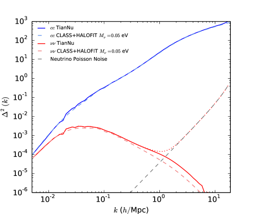
Figure 5: Dimensionless power spectrum $\Delta^{2}$ of $\delta_{c}$ and $\delta_{\nu}$ from the TianNu simulation and their nonlinear predictions. Poisson noise of neutrino particles shown in grey dashed line.

We output 21 checkpoints containing all CDM and neutrino positions and velocities. For our checkpoints, we store particles ordered by their coarse cell location. We then record the number of particles per coarse cell as a 1-byte integer, their fractional location across the cell as a 1-byte integer (e.g. for a coordinate that is 24.4883 $\simeq$ 24 + 125/256 we store “125”) per dimension. For velocities we record one 2-byte integer per dimension indicating the fraction of the maximum particle velocity with a resolution of $2^{-16}$. In total, CDM requires 10 bytes per particle and neutrinos 9.125 bytes per particle as opposed to the traditional 24 bytes per particle each (e.g. 6 coordinates each as a 4-byte float). Analysis and results in this paper are based on the checkpoint at redshift $z=0.01$. In Fig.5 we show the dimensionless power spectrum $\Delta^{2}\equiv k^{3}P(k)/2\pi^{2}$ of $\delta_{c}$ and $\delta_{\nu}$ in TianNu at $z=0.01$, as well as their theoretical predictions , where $P(k)$ is the power spectrum. One can see that the peak maximum at $k\simeq 0.04$ $h/{\rm Mpc}$ in the neutrino power spectra – corresponding to the neutrino free streaming scale – is well recovered both by the nonlinear prediction (red dashed line) and in the TianNu simulation (red solid line, with predicted Poisson noise subtracted). Another two scales of interest are $k\simeq 0.01$ $h/{\rm Mpc}$ where $\delta_{\nu}$ still traces $\delta_{c}$ and $k\simeq 0.5$ $h/{\rm Mpc}$ where the formations of halos take place. Our choice of simulation scale $L$ and enough neutrino particles prevent these three scales of interest from being contaminated by neutrino Poisson noise and being affected by the periodic boundary conditions of the simulation. Although baryonic physics is non-negligible on and below halo scales, neutrinos in a halo come from $\sim 100$ ${\rm Mpc}/h$, while CDM and baryons all come from $\sim 1$ ${\rm Mpc}/h$. Interaction of CDM and baryons should not affect neutrinos. Thus, the relative neutrino-rich and -poor properties is conserved and $\partial(\Delta r/r)/\partial\hat{\delta}_{\nu}$ should be unaffected. Additionally, the overall nature of our “differential” analysis cancels out the CDM and baryon effects, which are uncorrelated with neutrino excess, $\epsilon_{\nu}$.

Halo finding and matching.

The halo finding procedure uses a spherical overdensity approach. It searches for local maxima in a nearest-grid-point CDM density field with a threshold $\delta_{c}>100$. It then uses a parabolic interpolation to search for the precise maxima of the particles. These maxima are then inspected, largest $\delta_{c}$ first, and halo mass is accumulated in spherical shells surrounding the maxima until the mean density drops below $178$ times the mean density. After selection as a halo, the mass is removed to avoid double counting in the case of nearby maxima. For each halo, we record the total mass of the CDM particles contained within its radius , and its centre-of-mass position $\vec{x}$. We do not include neutrinos in the mass calculation. Nonetheless, we have checked that including neutrino particles in the mass count does not affect our final result.

In the matching of halos between TianNu and TianZero, we define a matched pair if the coordinates of the two halos are separated by less than 100 kpc/$h$ in their respective volumes, and if their masses vary by less than 10%. We are able to associate 98% of all halos between TianNu and TianZero in this way, corresponding to a total of 27 million pairs of halos in range $10^{13}\lesssim m_{h}/M_{\odot}\lesssim 10^{15}$.

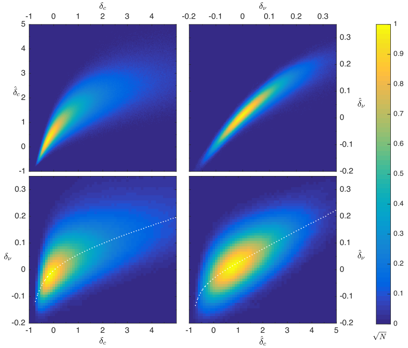
Figure 6: Correlations between simulated and/or reconstructed densities for CDM and neutrinos. The top two panels show simulation-reconstructed density field correlation $\hat{\delta}_{c}-\delta_{c}$ and $\hat{\delta}_{\nu}-\delta_{\nu}$. Bottom two panels show neutrino-CDM density correlations for simulated fields $\delta_{\nu}-\delta_{c}$ and reconstructed fields $\hat{\delta}_{\nu}-\hat{\delta}_{c}$.

Density reconstruction and correlation.

Here we analyze the degree to which $(\delta_{c},\delta_{\nu})$ can be reconstructed using linear theory. We compute local values of $\delta_{c}$ and $\delta_{\nu}$ within cubes of width 9.4 ${\rm Mpc}/h$ centered on the position of each halo in TianNu. We could have used the exact values of $\delta_{c}$ and $\delta_{\nu}$ extracted from the neutrino simulation, however these quantities are not directly observable. Instead, we linearly reconstruct both densities using the TianNu halo density field. This is done in an analogous manner to the velocity reconstruction in [20]. Halos are cloud-in-cell (CIC) interpolated to the same grid we used for particles to obtain the halo density field $\delta_{h}$. Then in Fourier space, we compute the temporary reconstructed fields

$$\hat{\delta}^{\dagger}_{i}(k)=\frac{T_{i}(k)}{T_{c}(k)}\frac{1}{b(k)}\delta_{h}(k),$$

where $i=c,\nu$ stands for CDM or neutrinos. $T_{i}(k)$ is the transfer function in Fourier space, and the bias $b(k)=P_{ch}(k)/P_{cc}(k)$, the ratio of CDM-halo cross power spectrum and CDM auto power spectrum measured in the simulation. Then we apply a low pass Wiener filter $W(k)$ to each of these $\hat{\delta}^{\dagger}_{i}(k)$ to get the reconstructed field $\hat{\delta}_{i}(k)=\hat{\delta}^{\dagger}_{i}(k)W(k)$, where the $W(k)$ is computed as:

$$W(k)=\frac{B(k)P_{ss}(k)}{P_{ss}(k)+N^{2}(k)}$$

where $N^{2}(k)=P_{ss}(k)-B^{2}(k)P_{rr}(k)$ and $B(k)=P_{rs}(k)/P_{rr}(k)$. Here $P_{ss}$ and $P_{rr}$ are the auto power spectra of the simulated and reconstructed density fields, respectively, and $P_{rs}$ is their cross power spectrum. An inverse Fourier transform gives us the density contrasts. We then proceed to cubically average these $\hat{\delta}$’s about the halo position so the resultant density field is constant over scales of $9.375$ ${\rm Mpc}/h$ (9 grid cells). We label the result $\hat{\delta}_{c}$ and $\hat{\delta}_{\nu}$ and stress to the reader that these are observable quantities. We have checked that computing $\hat{\delta}_{c}$ and $\hat{\delta}_{\nu}$ from TianZero halo catalog does not affect our result. The simulated density fields are computed via CIC interpolation of particles onto a uniform mesh containing $1152^{3}$ cells and then filtered in Fourier space by the same Wiener filter $W(k)$. Here we just label them $\delta_{c}$ and $\delta_{\nu}$.

In Fig.6 we show halo number density as functions of their reconstructed and/or simulated density fields. The top two panels show the quality of our reconstruction method. Halos are not perfectly distributed on single diagonal lines, but ideally reflect the correlation between simulated and reconstructed $\delta_{c}$’s or $\delta_{\nu}$’s. The Pearson’s $r$ for $\delta_{c}$ is $\rho_{c,c}=0.80$ and for $\delta_{\nu}$ is $\rho_{\nu,\nu}=0.95$. It is more difficult to predict $\delta_{c}$ since halos are modelled as unit point mass in the reconstruction and any sub-halo structures (1-halo term) are neglected. This directly leads to a suppression and large scatter in $\hat{\delta}_{c}$ when $\delta_{c}\gg 1$. $\delta_{\nu}$ is less affected by this as neutrinos do not contain much structure on small scales due to their thermal velocities. The bottom two panels show $\delta_{c}-\delta_{\nu}$ correlations for simulation and reconstructed fields. The right one is identical to Fig.2 in the main text. When we repeat our analysis with density contrasts from the simulation $(\delta_{c},\delta_{\nu})$ instead of halo reconstructed ones $(\hat{\delta}_{c},\hat{\delta}_{\nu})$, we find the best fit will be $\partial(\Delta r/r)/\partial\delta_{\nu}=(0.00283\pm 0.00105)\log_{10}(r/r_{\rm pivot})-(0.00260\pm 0.00023)$, and $r_{\rm pivot}=4.56\times 10^{5}$.

References

- [1] Cowan, C. L., Jr., Reines, F., Harrison, F. B., Kruse, H. W. & McGuire, A. D. Detection of the Free Neutrino: A Confirmation. Science 124, 103–104 (1956).
- [2] Danby, G. et al. Observation of high-energy neutrino reactions and the existence of two kinds of neutrinos. Phys. Rev. Lett. 9, 36–44 (1962). URL http://link.aps.org/doi/10.1103/PhysRevLett.9.36.
- [3] Fukuda, Y. et al. Evidence for oscillation of atmospheric neutrinos. Phys. Rev. Lett. 81, 1562–1567 (1998). URL http://link.aps.org/doi/10.1103/PhysRevLett.81.1562.
- [4] Ahmad, Q. R. et al. Direct Evidence for Neutrino Flavor Transformation from Neutral-Current Interactions in the Sudbury Neutrino Observatory. Physical Review Letters 89, 011301 (2002). nucl-ex/0204008.
- [5] Ahmad, Q. R. et al. Measurement of the rate of interactions produced by solar neutrinos at the sudbury neutrino observatory. Phys. Rev. Lett. 87, 071301 (2001). URL http://link.aps.org/doi/10.1103/PhysRevLett.87.071301.
- [6] Olive, K. A. & Particle Data Group. Review of Particle Physics. Chinese Physics C 38, 090001 (2014).
- [7] Planck Collaboration et al. Planck 2015 results. XIII. Cosmological parameters. ArXiv e-prints (2015). 1502.01589.
- [8] Laureijs, R. et al. Euclid Definition Study Report. ArXiv e-prints (2011). 1110.3193.
- [9] LSST Science Collaboration et al. LSST Science Book, Version 2.0. ArXiv e-prints (2009). 0912.0201.
- [10] Dawson, K. S. et al. The SDSS-IV extended Baryon Oscillation Spectroscopic Survey: Overview and Early Data. ArXiv e-prints (2015). 1508.04473.
- [11] Eisenstein, D. & DESI Collaboration. The Dark Energy Spectroscopic Instrument (DESI): Science from the DESI Survey. In American Astronomical Society Meeting Abstracts, vol. 225 of American Astronomical Society Meeting Abstracts, 336.05 (2015).
- [12] Abazajian, K. N. et al. Neutrino physics from the cosmic microwave background and large scale structure. Astroparticle Physics 63, 66–80 (2015).
- [13] Mead, A. J. et al. Accurate halo-model matter power spectra with dark energy, massive neutrinos and modified gravitational forces. MNRAS (2016). 1602.02154.
- [14] LoVerde, M. Spherical collapse in CDM. Phys. Rev. D 90, 083518 (2014). 1405.4858.
- [15] Castorina, E., Carbone, C., Bel, J., Sefusatti, E. & Dolag, K. DEMNUni: the clustering of large-scale structures in the presence of massive neutrinos. JCAP 7, 043 (2015). 1505.07148.
- [16] Brandbyge, J., Hannestad, S., Haugbølle, T. & Wong, Y. Y. Y. Neutrinos in non-linear structure formation - the effect on halo properties. J. Cosmology Astropart. Phys. 9, 014 (2010). 1004.4105.
- [17] Castorina, E., Sefusatti, E., Sheth, R. K., Villaescusa-Navarro, F. & Viel, M. Cosmology with massive neutrinos II: on the universality of the halo mass function and bias. J. Cosmology Astropart. Phys. 2, 049 (2014). 1311.1212.
- [18] Villaescusa-Navarro, F., Bird, S., Peña-Garay, C. & Viel, M. Non-linear evolution of the cosmic neutrino background. J. Cosmology Astropart. Phys. 3, 019 (2013). 1212.4855.
- [19] Harnois-Déraps, J. et al. High-performance P3M N-body code: CUBEP3M. Mon. Not. R. Astron. Soc. 436, 540–559 (2013). 1208.5098.
- [20] Inman, D. et al. Precision reconstruction of the cold dark matter-neutrino relative velocity from N -body simulations. Phys. Rev. D 92, 023502 (2015). 1503.07480.
- [21] Blas, D., Lesgourgues, J. & Tram, T. The Cosmic Linear Anisotropy Solving System (CLASS). Part II: Approximation schemes. J. Cosmology Astropart. Phys. 7, 034 (2011). 1104.2933.
- [22] Trujillo-Gomez, S., Klypin, A., Primack, J. & Romanowsky, A. J. Galaxies in CDM with Halo Abundance Matching: Luminosity-Velocity Relation, Baryonic Mass-Velocity Relation, Velocity Function, and Clustering. ApJ 742, 16 (2011). 1005.1289.
- [23] Klypin, A., Prada, F., Yepes, G., Hess, S. & Gottlober, S. Halo Abundance Matching: accuracy and conditions for numerical convergence. ArXiv e-prints (2013). 1310.3740.
- [24] Klypin, A., Prada, F., Yepes, G., Heß, S. & Gottlöber, S. Halo abundance matching: accuracy and conditions for numerical convergence. MNRAS 447, 3693–3707 (2015).
- [25] Berlind, A. A. & Weinberg, D. H. The Halo Occupation Distribution: Toward an Empirical Determination of the Relation between Galaxies and Mass. ApJ 575, 587–616 (2002). astro-ph/0109001.
- [26] Zheng, Z. et al. Theoretical Models of the Halo Occupation Distribution: Separating Central and Satellite Galaxies. ApJ 633, 791–809 (2005). astro-ph/0408564.
- [27] Li, Y., Hu, W. & Takada, M. Super-sample covariance in simulations. PRD 89, 083519 (2014). 1401.0385.