DEMNUni: The clustering of large-scale structures in the presence of massive neutrinos
Abstract
We analyse the clustering features of Large Scale Structures (LSS) in the presence of massive neutrinos, employing a set of large-volume, high-resolution cosmological N-body simulations, where neutrinos are treated as a separate collisionless fluid. The volume of 8, combined with a resolution of about for the cold dark matter (CDM) component, represents a significant improvement over previous N-body simulations in massive neutrino cosmologies. In this work we focus, in the first place, on the analysis of nonlinear effects in CDM and neutrinos perturbations contributing to the total matter power spectrum. We show that most of the nonlinear evolution is generated exclusively by the CDM component. We therefore compare mildly nonlinear predictions from Eulerian Perturbation Theory (PT), and fully nonlinear prescriptions (halofit) with the measurements obtained from the simulations. We find that accounting only for the nonlinear evolution of the CDM power spectrum allows to recover the total matter power spectrum with the same accuracy as the massless case. Indeed, we show that, the most recent version of the halofit formula calibrated on CDM simulations can be applied directly to the linear CDM power spectrum without requiring additional fitting parameters in the massive case. As a second step, we study the abundance and clustering properties of CDM halos, confirming that, in massive neutrino cosmologies, the proper definition of the halo bias should be made with respect to the cold rather than the total matter distribution, as recently shown in the literature. Here we extend these results to the redshift space, finding that, when accounting for massive neutrinos, an improper definition of the linear bias can lead to a systematic error of about 1- in the determination of the linear growth rate from anisotropic clustering. This result is quite important if we consider that future spectroscopic galaxy surveys, as e.g. Euclid, are expected to measure the linear growth-rate with statistical errors less than about at .
1 Introduction
In the CDM cosmological model the three active neutrinos of the standard model of particle physics are assumed to be massless. Nevertheless, already in 1998 the Super-Kamiokande collaboration presented evidence of neutrino oscillations [1], indicating that at least two neutrinos are massive, and, more recently, new neutrino oscillation experiments seem to exclude a vanishing flavor mixing angle at more than 10 (see, e.g. [2, 3]). Indeed, the study of the effects of neutrino masses on cosmological observables is of particular relevance for two, distinct, reasons. First, the absolute neutrino mass scale remains unknown and, in this respect, cosmology plays a key role in its determination, being gravity sensitive to the total neutrino mass, , rather than to the mass splitting. Second, an accurate description of massive neutrino effects on LSS is required to avoid systematic errors in the determination of cosmological parameters, as the dark energy density and equation of state, whose measurements represent one of the main goals of current and future cosmological experiments.
Massive neutrino cosmologies have been extensively studied in the literature (see [4, 5] for a review). In particular the linear perturbation theory in the presence of massive neutrinos is well understood and it is widely used to derive constraints on and other cosmological parameters, from present and future CMB and galaxy surveys observations [6, 7, 8, 9, 10, 11, 12, 13, 14, 15, 16, 17, 18, 19, 20, 21, 22, 23]. However, the increasing precision of cosmological parameter measurements further requires an accurate description of nonlinear corrections, which can be obtained by means of a direct analysis of the output of N-body simulations accounting for a massive neutrino component. This kind of simulations turns to be computationally very expensive and quite challenging if a good mass resolution and a large box size are required at the same time in order to build realistic mock catalogues for present and future galaxy and weak lensing surveys.
The “Dark Energy and Massive Neutrino Universe” (DEMNUni) simulation project presented in this and in the companion paper [24], addresses in a consistent way the problem of structure formation in massive neutrino cosmologies, and represents the state of the art of neutrino simulations in terms of volume and mass resolution. At present, as explained in more details in §3 below, these simulations include a baseline CDM model and three cosmologies characterised by different values of , with all the cosmologies sharing the same total matter density , as well as the same amplitude of primordial curvature perturbations. In the near future, the DEMNUni set will be extended with the inclusion of an evolving dark energy background, with different equations of state , in order to study the degeneracy between the neutrino mass and at the nonlinear level.
This work focuses on the analysis of the clustering features of LSS in massive neutrino cosmologies, as extracted from the DEMNUni simulation set, including, in the first place, an accurate comparison of the nonlinear total matter power spectrum with the most recent predictions in PT, over the range of scales where such predictions are expected to significantly improve over linear theory. To this end we will separately consider the clustering of the CDM and neutrino components as well as their cross-correlation, following previous indications that such distinctions are quite relevant for an accurate description of gravitational instability in these cosmological models (see, e.g. [25, 26, 27]). At the same time, we will test different implementations of popular fitting formulae such as halofit [28, 29, 30] describing the nonlinear regime. A specific study of non-Gaussian aspects of the matter distribution in massive neutrinos cosmologies is left to future work [31].
In addition, we will revise previous results on the abundance and clustering of dark matter halos, taking advantage of the large volume and mass resolution provided by the DEMNUni simulations. In this respect, our results provide further evidence that a description in terms of cold (rather than total) dark matter perturbations is indeed required for the extension of common fitting functions for the halo mass function to the case of massive neutrinos. In this respect, despite the significant systematic effect that the wrong assumption would lead to the interpretation of cluster abundance observations [32], these early indications have been so far ignored in the analysis of relevant data-sets (e.g. [33]). We believe that, whether or not particle-based neutrino simulations provide an faithful description of reality, such systematic uncertainties should be at the very least accounted for in any exhaustive error budget. Similar considerations can be extended to the interpretation of galaxy power spectrum measurements where the assumption of a constant linear bias with respect to the CDM or total matter power spectrum can lead to quite different constraints on the total neutrino mass [26]. In this work, for the first time we extend from real to redshift space our results on halo clustering in the presence of massive neutrinos, providing a first insight into possible, additional systematic effects due to erroneous assumptions in the modelling of galaxy clustering anisotropies in massive neutrino scenarios.
This paper is organised as follow. In §2 we give a brief description of linear perturbation theory in the presence of massive neutrinos. In §3 we present the N-body runs and the details of the numerical setup. In §4 we present our measurements of all the components to the matter power spectrum, along with comparison with PT results and popular fitting formulae. In §5 and §6, we focus our attention on the mass function and the power spectrum of halos both in real and redshift space. Finally, in §7 we summarise the main results of the present work and draw our conclusions, highlighting several applications of the DEMNUni simulations to the testing of different observables and probes in the context of massive neutrinos cosmologies.
2 Massive neutrinos perturbations
Massive neutrinos are considered hot dark matter, since they decouple in the early Universe as relativistic particles, just before the onset of Big Bang Nucleosynthesis, and become non-relativistic only at later times. This transition happens when the neutrino temperature drops below the value of their mass at redshift [34]
| (2.1) |
After this time they contribute to the total energy density of the Universe as dark matter so that the total matter energy density is given by
| (2.2) |
where, in addition to the CDM and baryon components, accounts for the energy density associated to the massive neutrino component. Since we will consider scales much larger than the Jeans length of baryons, in what follows we will define as the density corresponding to the sum of CDM and baryon densities, and, for simplicity, will generically refer to it as a single “CDM” contribution, denoted by the subscript “c”. It can be shown that is proportional to the total neutrino mass as
| (2.3) |
where the proportionality factor depends on the assumed photon temperature and neutrino to photon temperature ratio and it should be evaluated numerically in the most general case [35]. As a result, at late times, i.e. , the effect of neutrinos on the expansion rate of the Universe is completely degenerate with a change of the CDM and baryon components.
On the other hand, at the perturbation level massive neutrinos have a peculiar effect on matter density fluctuations. Defining the density contrasts for neutrino and CDM respectively as and , where the total mass density is , being the total background matter density, we can write
| (2.4) |
where represents the neutrino fraction defined as . It follows that the total matter power spectrum can be written as the sum of three contributions corresponding respectively to the CDM power spectrum, , the neutrinos power spectrum, , and the cross-power spectrum between CDM and neutrinos, , that is
| (2.5) |
which shows that the neutrino fraction has a direct impact on the total matter power spectrum by modifying the relative contributions of the two components. Eqs. (2.2) to (2.5) introduce the notation adopted throughout the rest of the paper.
Over the age of the Universe, neutrinos travel an average distance that depends on their thermal velocity and, in turn, on their mass. This free streaming length determines the scale below which neutrinos density perturbations are washed-out, and is given by (see, e.g. [5])
| (2.6) |
Notice that, for particles becoming non-relativistic during matter domination, as it is usually the case for neutrinos, the comoving free streaming length, , is actually decreasing in time, and therefore assumes the largest value at the time of the non-relativistic transition. This peculiar distance corresponds to the wave-number
| (2.7) |
This scale is typically larger than the scale at which nonlinear effects manifest themselves at low redshifts. At any redshift, scales larger than are affected by the presence of massive neutrinos, and, in first approximation, we can write
| (2.8) |
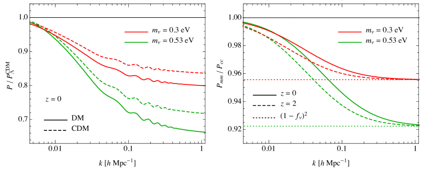
while the exact value of the damping scale will retain a residual redshift dependence. In the left panel of Figure 1 we plot the ratio for eV at redshifts , showing the two asymptotic regimes of Eq. (2.8). On very large scales the ratio goes to one, while at small scales it approaches regardless of the redshift. Intermediate scales are instead affected by the actual value of the free streaming wave number , and by its redshift dependence.
It can be shown [36] that, with respect to the massless case, the total linear power spectrum, , in massive neutrino scenarios is asymptotically suppressed at by a constant factor on scales
| (2.9) |
while from Eq. (2.8) and Eq. (2.5), it follows that the suppression for the CDM power spectrum, , is given by a factor . The difference in the suppression between the two power spectra is shown in the right panel of Figure 1.
3 Simulations
The DEMNUni simulations have been conceived for the testing of different probes, including galaxy surveys, CMB lensing, and their cross-correlations, in the presence of massive neutrinos. To this aim, this set of simulations is characterised by a volume big enough to include the very large-scale perturbation modes, and, at the same time, by a good mass resolution to investigate small-scales nonlinearity and neutrino free streaming. Moreover, for the accurate reconstruction of the light-cone back to the starting redshift of the simulations, it has been used an output-time spacing small enough that possible systematic errors, due to the interpolation between neighbouring redshifts along the line of sight, result to be negligible.
The simulations have been performed using the tree particle mesh-smoothed particle hydrodynamics (TreePM-SPH) code gadget-3, an improved version of the code described in [37], specifically modified in [38] to account for the presence of massive neutrinos. This version of gadget-3 follows the evolution of CDM and neutrino particles, treating them as two distinct collisionless fluids. For the specific case of the DEMNUni simulations, a gadget-3 version, modified for OpenMP parallelism and for memory efficiency, has been used to smoothly run on the BG/Q Fermi cluster.
Given the relatively high velocity dispersion, neutrinos have a characteristic clustering scale larger than the CDM one. This allows to save computational time by neglecting the calculation of the short-range tree-force induced by the neutrino component. This results in a different scale resolution for the two components, which for neutrinos is fixed by the PM grid (chosen with a number of cells eight times larger than the number of particles), while for CDM particles is larger and given by the tree-force (for more details see [38] ). This choice does not affect the scales we are interested in, since, as shown in [39], the application of the short-range tree force to neutrino particles is required only to describe the neutrino density profile inside massive halos at low redshifts. In this work we are not considering this kind of analysis on such small scales.
Each DEMNUni run starts at redshift , and is characterised by a comoving volume of , filled with 20483 dark matter particles and, when present, 20483 neutrino particles. Given the large amount of memory required by the simulations, baryon physics is not included. Nevertheless, since we are looking for deviations from a fiducial reference CDM model, it is expected that baryon feedback cancels out when considering relative effects, i.e. the massive with respect to the massless neutrino case. In addition we expect also that any additional effect produced by the interplay of neutrinos with baryon physics should be of higher order. This is supported also from [40] which shows that the neutrino induced suppression in the total matter power spectrum is very much the same also when neutrinos are considered in the presence of baryons. Therefore, our choice should not affect the results presented in this work.
| [eV] | |||||||
|---|---|---|---|---|---|---|---|
| S1 | 0.00 | ||||||
| S2 | 0.17 | ||||||
| S3 | 0.30 | ||||||
| S4 | 0.53 |
We have produced a total of four different DEMNUni simulations, choosing the cosmological parameters according to the Planck 2013 results [41], namely a flat CDM model generalised to a CDM , i.e. a massive neutrino model, by varying only the sum of the neutrino masses over the values eV (and consequently the corresponding values of and , while keeping fixed and the amplitude of primordial curvature perturbations ). Table 1 provides a summary of the cosmological parameters that characterise the different runs. It shows as well the derived quantities and corresponding to the r.m.s. of perturbations on spheres of , computed respectively for the total and CDM matter components, and the CDM and neutrino mass particle resolutions, which vary according to the value of and .
The simulations are characterised by a softening length kpc, and have been run on the Fermi IBM BG/Q supercomputer at CINECA111Consorzio Interuniversitario del Nord-Est per il Calcolo Automatico, Bologna, Italy: http://www.hpc.cineca.it/services/iscra., employing about 1 Million cpu-hrs per simulation (including the production of halo and sub-halo catalogues). For each simulation, 62 outputs have been produced, logarithmically equispaced in the scale factor , in the redshift interval , 49 of which lay between and . For each of the 62 output times, it has been produced on-the-fly one particle snapshot, composed by both CDM and neutrino particles, one 3D Cartesian grid of the gravitational potential, , and one 3D cartesian grid of its time derivative, , with a mesh of dimension 40963 that covers a comoving volume of 2 Gpc, for a total of about 90 TB of data per simulation. In addition, in order to build parent-halo catalogues, the simulation outputs have been first processed with the friends-of-friends (FoF) algorithm included in the gadget-3 package. The code is applied only to CDM particles with linking length set to 0.2 times the mean inter-particle distance. A minimum number of 32 particles to identify a structure has been assumed, fixing the minimum parent-halo mass to . The FoF catalogues have subsequently been processed with the subfind algorithm [42, 43], which identifies locally overdense, gravitationally bound regions within an input parent halo. With this procedure some of the initial FoF parent halos are split into multiple sub-halos, with the result of an increase of the total number of identified objects, and of a lower minimum mass limit. Here, a minimum number of particles has been adopted in order to constitute a valid sub-halo. Moreover, by means of a specific routine included in the subfind algorithm, spherical overdensity halo catalogues have been produced, and, in particular, for each halo the value of has been computed; this is defined as the radius enclosing a matter (CDM+neutrinos) density equal to 200 times the mean density of the Universe at redshift , and the corresponding mass in terms of . We stress here that all the post-processing has been modified to take the neutrino component properly into account.
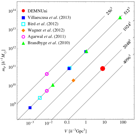
Figure 2 presents a comparison of the DEMNUni simulations to previous N-body simulations with massive neutrino particles, in terms of the CDM particle mass resolution and simulation volume . Diagonal grey lines indicate the number of CDM particles. With respect to previous simulations, the DEMNUni suite represents an improvement of about an order of magnitude in terms of particle number (only [44] considered a larger box, but with considerably smaller mass resolution).
4 Matter power spectra
As shown in §2, the shape of the linear power spectrum is quite sensitive to the value of neutrino masses, and this dependence becomes even stronger in the mildly and fully nonlinear regimes [44, 40]. Taking advantage of the large DEMNUni simulations volume, in this section we aim at testing the accuracy of current analytical predictions for the nonlinear matter power spectrum, , in the presence of massive neutrinos. To this end, we measure individually the different components to in Eq. (2.5), from very large scales, , down to fully nonlinear scales, , and compare these measurements with PT predictions, in the mildly nonlinear regime, and fitting functions as halofit [45, 30], in the fully nonlinear regime222While the mass resolution of the DEMNUni simulations would allow to look at much smaller scales, of the order of , we do not investigate this regime since it is dominated by baryon physics [46, 47, 48, 49, 50].. The goal here is to understand if possible departures from the linear regime of neutrino perturbations have to be taken into account for precision cosmology at the % level.
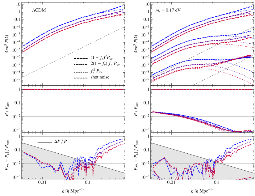
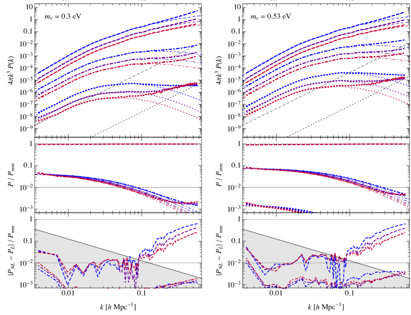
Before proceeding to the comparison with the nonlinear, analytical predictions, however, we take a look at each component and its relative contribution to the nonlinear measured from the simulations. Figures 3 and 4 show the CDM auto power spectrum, (dashed curves), the neutrino auto power spectrum, (dotted curves), and the cross CDM-neutrino power spectrum, (dot-dashed), as extracted from the simulations (thick curves), and the corresponding linear predictions (thin curves). Each plot corresponds to a different value of the neutrino mass in the simulations. Within each plot, the top panel shows the adimensional power spectrum, , the middle panel the ratio of each contribution to , in the nonlinear and linear cases, and the bottom panel shows the ratio , i.e. the difference between each measured nonlinear component, , in Eq. (2.5), and the corresponding linear prediction, , compared to the nonlinear . All the measurements at redshifts are shown with different shades varying from blue to red. Dashed and dotted grey lines on the top panels show the shot-noise contributions to the CDM and neutrinos power spectra, respectively. The shaded area in the bottom panel show the region below the 1-, Gaussian uncertainty on , given by , being the fundamental frequency of the simulation box (the shot-noise contribution to the variance is ignored for simplicity).
In the linear regime, , most of the power comes from the CDM component, with the cross power spectrum term accounting roughly for a 10% of the total , and the neutrinos being already negligible (see middle panels of Figures 3 and 4). On nonlinear scales, from the lower panels we notice that most of the nonlinear contribution to is still given by , which is the only component significantly deviating from the linear prediction, while the other two terms remain linear, and, therefore, less and less important as we move to smaller scales333Let us notice that measurements of the neutrino auto power spectrum and neutrino-cold matter cross power spectrum shown in both Figures 3 and 4, present a spurious contribution at small scales not to be confused with a residual shot noise component. Such contribution, which scales roughly (but not exactly) as , is due to the neutrino velocity distribution and it does not grow with time, so that at low redshift is overtaken by the expected neutrino power spectrum. A detailed discussion of numerical issues associated with the set-up of the initial conditions will be discussed in a forthcoming work [51].. It should be kept in mind that each contribution in Figures 3 and 4 is multiplied by the proper power of or , with . We therefore conclude that, on the scales probed by the DEMNUni simulations, and considering the present constraints on the sum of neutrino masses, the total nonlinear matter power spectrum, in massive neutrino cosmologies, can be described at the 1% level by accounting for the nonlinear evolution of CDM perturbations alone, while adopting the linear prediction for the other components. This result will be useful for analytical predictions of the nonlinear discussed in the next sections.
4.1 Perturbation Theory
For the first time in the literature, the large volume of the DEMNUni simulations gives us the possibility to measure the matter power spectrum in neutrino cosmologies at the 1% accuracy level, on a very large range of scales, allowing a test of PT predictions at the accuracy level required by current and futures galaxy surveys.
Several works in the literature have discussed the effects of massive neutrinos in cosmological perturbation theory beyond the linear level [52, 53, 54, 55, 56, 57, 10, 58, 27]. In these descriptions, the neutrino component is treated, similarly to the CDM one, as a single perfect fluid, fully characterised in terms of its density and velocity divergence (see, however, [59, 60] for a multiple-flow approach to the evolution of neutrino perturbations). The main difference with respect to the CDM case is represented by an effective sound speed modifying the Euler equation for the neutrino component, and accounting for the neutrino velocity distribution. The first consequence, at the linear level, is a scale-dependent linear growth factor, , for both the CDM and neutrino components. However, the perfect-fluid approximation fails to provide an accuracy for the neutrino power spectrum below the 10% level [57]. Nonetheless, as shown in §4, since the neutrino contribution to the total matter power spectrum is order of magnitudes smaller than the CDM one, such discrepancies on the neutrino component alone do not affect significantly the CDM and total matter power spectra. Therefore, we will assume the two-fluid approximation for all the comparisons of analytical versus numerical results in this section.
In addition, even if in the mildly nonlinear regime the effective sound speed affects as well the mode-coupling at all the orders of the perturbative expansion, we will follow the same approach adopted by [54]. They have shown that limiting the neutrino-induced scale-dependence to the linear growth factor alone (and, therefore, the use of standard EdS- like kernels in the perturbative expansion) proves to be a quite good approximation to the full PT solution for the nonlinear CDM field, on scales where PT is expected to be accurate.
Finally, we will make the additional approximation, already proposed in [52], of describing the neutrino perturbations by means of their linear solution. While this is not per se a good assumption [27, 58], it does provide the correct neutrino contribution to the total matter power spectrum on the (large) scales where such contribution is relevant.
As a starting point for future, more accurate comparisons, we will consider, therefore, the following perturbative prediction for the total matter power spectrum
| (4.1) |
Here, the contribution represents the nonlinear power spectrum predicted in perturbation theory along the lines of [54], i.e. it is computed in terms of its linear counterpart, , which provides the correct linear scale-dependence of the growth factor, but assumes the standard EdS nonlinear kernels in the perturbative expansion. Differently from previous works, however, we do not only consider standard, one-loop corrections to , but we take into account also standard PT two-loop corrections, as well as the “regularised” predictions based on the multi-point propagator expansion of [61], computed using the RegPT code of [62]. Since the RegPT code does not account for the evolution of the scale-dependent linear growth in massive neutrino models, we produce all the predictions at by providing the corresponding -input linear power spectrum as a “fake input” required by the code.
While this is not the most rigorous approach, it represents a practical application, to massive neutrino scenarios, of available tools developed within the CDM framework. As we will see, the gain in accuracy achieved by recent resummation schemes, applied here to the CDM component alone, might compensate for the crude approximations that this approach implies. Clearly we are only considering predictions for the CDM and total matter power spectra, as these statistics are the relevant ones for galaxy clustering and weak lensing observations.
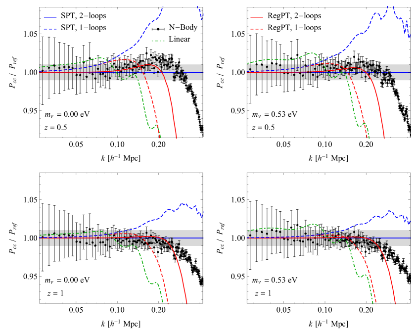
In Figure 5 we show the perturbative results against the measurements at , and for eV. Error bars are the theoretical expectation for a Gaussian field, that is
| (4.2) |
where is the fundamental frequency of the simulation box, being its linear size, and is the particle number density accounting for the shot-noise component444The relatively small scatter of data points with respect to the error bars is due to the specific seed chosen for the random number generator used for the set-up of the initial conditions [63]..
Let us first notice that, in the CDM case (left panels in Figure 5), the two-loops standard PT does not provide a good fit to the data at low redshifts [64], while it reproduces fairly well the simulation measurements at . Analytic predictions are 1% accurate at , up to a maximum wave-number 555It is worth noticing that the agreement may also depend on the simulation mass resolution; we expect that much higher resolutions lead to more power at small scales [65]..
Turning our attention to the CDM power spectrum in massive neutrino cosmologies (right panels in Figure 5), at we find approximately that the accuracy is recovered up to a value of very close to the CDM case. On the other hand, at lower redshifts, , we notice that, with respect to the massless case, PT predictions are in better agreement with the measurements extracted from the DEMNUni simulations. This is a consequence of the fact that, due to massive neutrino free streaming, the nonlinear evolution of CDM perturbations is suppressed, and therefore the range of scales in which PT corrections show the same accuracy as in standard CDM cosmologies increases with , i.e. with the relative contribution of the total neutrino mass to . In addition, since, massive neutrino free streaming has an impact already at the linear level, these models are characterised by a lower value of (and ) than a CDM universe with the same .
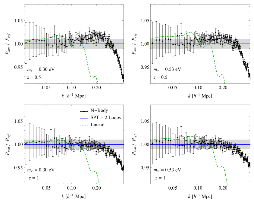
Given a prediction for the CDM power spectrum accurate at the 1% level up to a given , we check if the perturpative approach of Eq. (4.1) reproduces, with the same level of accuracy, the total matter power spectrum measured from the simulations. The results are illustrated in Figure 6, which shows that, indeed, the linear treatment of the and contributions to the total proves to be a very good approximation. The difference in the accuracy of the predictions between the eV (left panels) and the eV (right panels) cases is again mainly due to the different values of and, therefore, to the different effect of neutrino free streaming on dark matter perturbations, according to the total neutrino mass: for a given value of , a larger value of not only increases the relative amount of neutrino perturbations that are washed out below the free streaming scale, , consequently reducing the contribution of and to the total , but also decreases the factor in front of in Eq. (4.1), where the nonlinear evolution of is in turn suppressed, with respect to the massless case, by the action of the total gravitational potential sourced both by CDM and massive neutrinos. Apart from inducing a scale-dependence of the linear growth factors for CDM and total matter, the main direct product of this physical mechanism is represented by a lower amplitude of linear perturbations at , where , and , for eV, respectively. We will show in §4.2 that, on scales much smaller than the so-called turn-over scale, beyond the mildly nonlinear regime, , where the growth factor scale-dependence induced by neutrino free streaming approaches its asymptotic value depending only on (see Eq. (6.12) in §6.2), the effect of massive neutrinos on and mostly reduces to a mere rescaling of the power spectra in the massless case, according to the values of and .
Recently the BOSS collaboration released new constraints on neutrino masses based on measurements of the galaxy power spectrum multipoles in redshift space [21] at the mean redshift . The BOSS analysis was based on a prediction for the total matter power spectrum computed applying standard PT directly to the linear . The outcome of such a calculation, in principle even less theoretically justified than our crude assumptions, is very similar to our results obtained via Eq. (4.1); we have checked that any difference between the two approaches stays below the 1% level at the scales relevant for current observations.
A test somehow similar to the one presented here is shown in [66], where the authors compare different PT predictions, including the Time-RG method of [67, 55], to simulations of CDM particles, modifying only the background evolution and the initial conditions to account for free streaming massive neutrinos. They show that PT predictions are in agreement with the measurements of CDM power spectra, extracted from their CMD simulations, at the % level, over a similar range of scales as tested in this work. However they assume a scale-independent growth rate to rescale back the late time () CDM power spectrum, , to the initial redshift of the simulations. By doing so, the linear dynamics cannot be correctly recovered at any other than .
Finally, the crucial results of this section rely on the discussion of §4 and the measurements shown in Figures 3 and 4, that is the contributions from the two terms, other than , entering Eq. (4.1), and in particular from the cross power spectrum , always remain negligible compared to on nonlinear scales, at least for the level of accuracy requested for PT to be useful.
4.2 Fitting functions
Given the limitations of the perturbative approaches, it is sometimes convenient and/or sufficient to resort to fitting functions for the nonlinear matter power spectrum. In this section we see how the approximation of linear evolution for neutrino perturbation can be applied as well to the halofit prescription [45].
The halofit formula, originally based on stable clustering considerations [68, 69], provides a mapping between the linear power spectrum and the nonlinear one, which in turn depends on few cosmological parameters, e.g., , and several free parameters determined by comparisons against measurements from N-body simulations. A new, more accurate, version of the fitting formula has been recently presented by [30]. The revised formula is expected to be accurate at the 5% level for and , while it degrades to the 10% level for and .
In the context of massive neutrinos cosmologies, Ref. [40] provided corrections (controlled by a few, additional parameters) to the original halofit formula, in order to account for neutrinos effects on the nonlinear total matter power spectrum666The massive neutrino corrections of [40] have been implemented, along the revised version of [30], in the most recent versions of the camb [70] and class [71] codes.. However, as shown in Figures 3 and 4, nonlinear corrections to the cross power spectrum between CDM and neutrinos are below the percent level, therefore we wonder if, similarly to Eq. (4.1), a fitting formula for the total matter power spectrum, , could be given in terms of the linear predictions, and , and the halofit fitting formula applied directly to the linear CDM power spectrum, , that is
| (4.3) |
Here , where the halofit mapping, , between linear and nonlinear power spectra does not account for additional corrections due to massive neutrino physics.
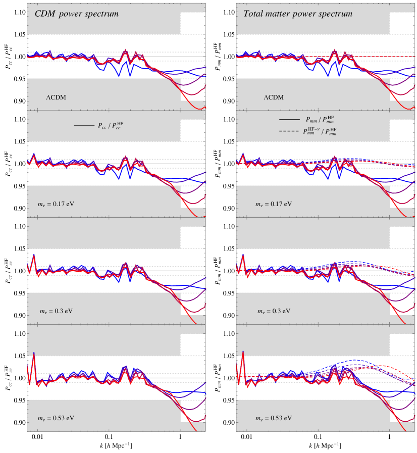
In the left column of Figure 7 we show the ratio of the measured CDM power spectrum, , to the prediction, . Each row corresponds to a distinct value of , while each panel shows the value of this ratio at redshifts , with colour shades ranging from blue to red. The shaded areas denote the regions beyond the accuracy claimed for the revised formula of [30]. The left panels of Figure 7 show, indeed, not only that provides the expected accuracy, but that it works equally well for all the considered values of the total neutrino mass. This is essential to justify our assumption of applying the halofit mapping to the CDM component alone. Here, we stress again that the version of halofit employed for does not include any effect due to massive neutrinos on the CDM clustering, since here we use the halofit version developed by [30] in the CDM framework. This result is similar to that obtained in §4.1 for perturbation theory, and it is a crucial step before checking the validity of the assumptions made in Eq. (4.3).
The right column of Figure 7 presents the ratio of the measured total matter power spectrum, , to the prediction of Eq. (4.3). In addition, dashed curves show the inverse ratio of to the specific halofit extension to massive neutrino cosmologies of [40], denoted as . We notice that the simple prescription of Eq. (4.3), while avoiding introducing additional parameters to the fitting formula of [30], remains well within the expected halofit accuracy. On the other hand, the discrepancies between the prediction of Eq. (4.3) and the fit of [40] are within 4%, with the latter ad-hoc fit not improving particularly over the former.
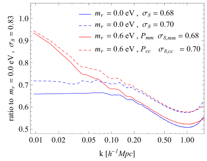
Here we would like to make some final considerations. The results of this section rely on the fact that, in the first place, in the absence of strong baryon physics, on scales much beyond the mildly nonlinear regime, , where the linear growth factor scale-dependence induced by neutrino free streaming approaches its asymptotic value, the extent of the nonlinear evolution of the power spectrum can be accounted for via the amplitude of the linear power spectrum, regardless of the physical mechanism responsible for the amplitude itself. In other terms, on nonlinear scales, we expect a similar behaviour for the nonlinear matter power spectrum evolved from a linear power spectrum suppressed by massive neutrino free streaming, as from a different linear power spectrum with a lower, primordial normalisation. This assertion can be easily tested with N-body simulations and the results are shown in Figure 8, which makes use, however, of measurements from the simulations described in [72, 73]. The plot shows ratios, with respect to the matter power spectrum in a given CDM cosmology with , of the matter power spectrum in other CDM cosmologies (with different normalisations ), and of the CDM and total matter power spectra in massive neutrino cosmologies, where either the value of or are matched to the CDM ones. We observe that on nonlinear scales, , a CDM model with a given is nearly indistinguishable from a massive neutrino model with the same value for . A lower agreement is found when the match is done in terms of , i.e. in terms of the normalisation of the linear total matter power spectrum, since the relevant nonlinear evolution is given by CDM perturbations, and the amplitude normalisation can not take correctly into account the contribution from remaining linear neutrino perturbations (this should be taken into consideration especially in weak-lensing analyses, which probe directly the total matter power spectrum). This result represents the well known degeneracy between and at small scales, and implies that the enhanced, nonlinear suppression of the matter power spectrum on nonlinear scales can be obtained tuning the normalisation of the linear one, without resorting to peculiar effects of massive neutrinos. Nonetheless, here we stress that, such kind of degeneracy can be broken when observing the power spectra on a much larger range of scales, , by means of future large sky galaxy surveys as, e.g., Euclid.
5 Halos mass function
The abundance of massive clusters as a function of redshift is a key cosmological probe for neutrino mass measurements [74, 75, 76]. In particular, massive neutrinos could alleviate the tension between the value of inferred from the primary CMB anisotropies [41, 77] and the one obtained from low redshift probes [18, 19, 32, 78, 79, 33, 80, 81]. A careful calibration of the halo mass function in simulations with a massive neutrino component is, therefore, required to avoid systematic effects in the determination of cosmological parameters.
The overall larger volume and higher mass resolution of the DEMNUni simulations with respect to previous studies (see Figure 2) allow an improved analysis of the abundance of massive clusters over several decades in mass. In this work, we identify halos in two different ways: using a Friends-of-Friends (FoF) algorithm with linking length equal to times the mean inter-particle distance, and with the SUBFIND-SO code included in the gadget package, which identifies halos whose spherical overdensity is times the mean background matter density, , as already mentioned in §3. FoF halo masses have been corrected following the empirical prescription by [82], and, for the present analysis, no halos with less than particles have been considered.
The halo mass function, i.e. the number density of halos of mass between and , is often expressed as
| (5.1) |
where most of the cosmological information is encoded in the variance of the matter distribution in the linear regime
| (5.2) |
smoothed on the scale with a Top-Hat filter in real-space 777To partially remove volume effects we use the fundamental frequency of the box, , as the lower integration limit in Eq. (5.2). . The function can be either predicted in the Press-Schechter framework [83] (see [84, 85] for recent results) or fitted to numerical simulations (see, e.g. [86, 87, 88]). The smoothing scale and the halo mass are related by the choice of the filter , and, in the Top-Hat case, is given by
| (5.3) |
Let us notice that in Eq. (5.1) as in Eq. (5.3), in the case of massive neutrino models, we need to use the background density of the cold (rather than total) matter component to define halo masses, since, as largely shown in the literature, the contribution of neutrinos (both bounded and unbounded) to the mass of CDM halos is completely negligible [44, 89, 25].
Another potential ambiguity in massive neutrino scenarios is that the variance in Eq. (5.1) could in principle be computed for cold or total matter perturbations. However, as shown in [25, 26], the halo mass function is well described by analytic predictions, and by common fitting functions developed in the context of CDM cosmologies, only if , i.e. the variance of the matter distribution is computed from the cold matter linear power spectrum . Here we summarise the physical mechanism behind this choice, referring the reader to [25, 26, 90, 91] for further details. In the spherical collapse model, assuming general relativity, the evolution of a region is controlled by the amount of mass inside its initial volume. For a Gaussian random field, as the linear density field , a natural choice to describe the system is therefore its variance smoothed on the scale associated to the initial region, . Due to the tiny value of neutrino masses, the scale is much smaller than the free streaming length of massive neutrinos , typically tens of Megaparsec, and therefore neutrino perturbations are vanishingly small inside the collapsing region. This implies that should be computed using the CDM plus baryon perturbations only. A similar argument applies to the critical overdensity required for collapse at a given redshift, , that depends on neutrino masses only through their effect on the background evolution [25]. Note that always (see Figure 1) implying that for a given cosmology, using in the computation of the mass function leads to predicting more halos than using (see [92] for implications in galaxy cluster counts observations). Of particular importance is that, as shown in [26], the universality of the function with respect to different cosmologies is recovered only for .
 |
 |
 |
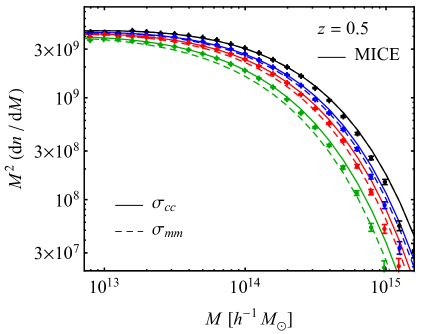
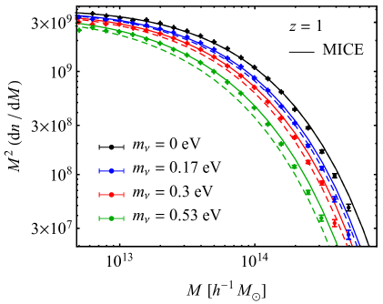
In Figure 9 we show the suppression of the FoF halo abundance due to free streaming massive neutrinos. The points show measurements from the DEMNUni simulations, at two redshifts , while the theoretical predictions are obtained in terms of the fitting formula of [87] as a function of (continuous curves) and (dashed curves). Let us notice that the volume and mass resolution of the DEMNUni simulations allow to recover the mass function of the FoF halos on a quite large range of scales, .
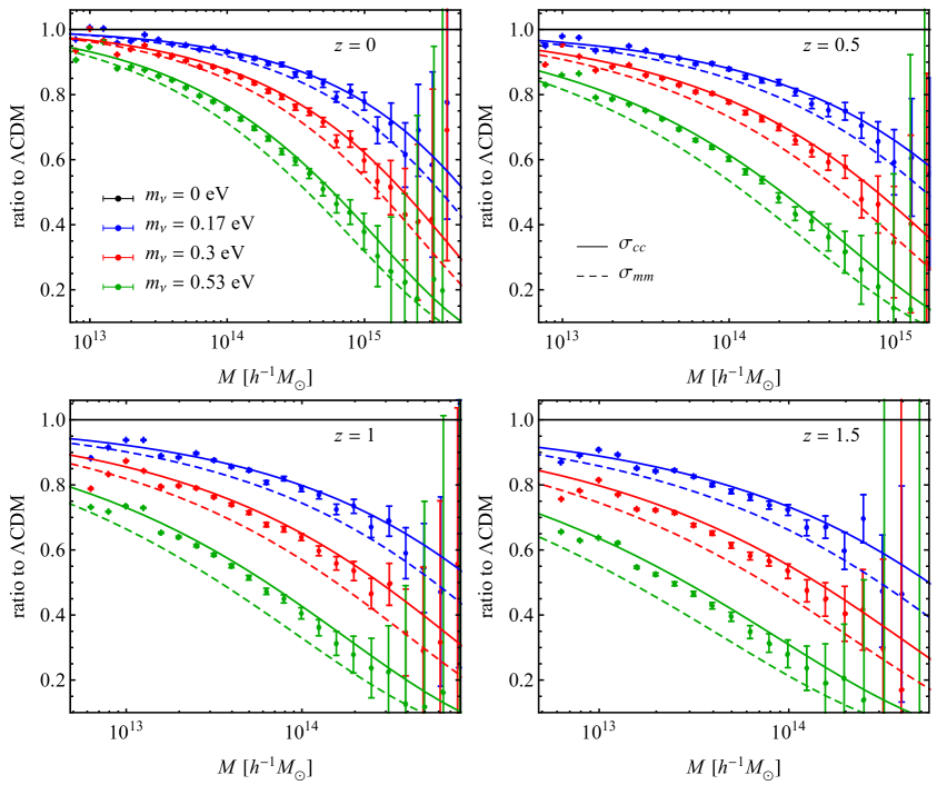
As a further inspection, in Figure 10 we show the ratios, over the CDM case, of the FoF halo mass function measured from the DEMNUni simulations at four different redshifts, . Again, we compare these measurements to the predictions from the MICE fit to FoF halos in [87]. Note that the MICE fit has been obtained using simulations of CDM cosmologies alone, and it is non-universal in redshift, i.e. does present an explicit redshift dependence on top of the one.
For the massive neutrino cosmologies we find that the cold matter prescription, with and in Eq. (5.1), reproduces very well the measurements when the MICE formula is assumed for the function . In fact, we find the same level of agreement encountered for the CDM model, therefore showing the same level of non-universality with respect to redshift. At high masses the measurements in the simulations drop below the MICE fit, because of the smaller volume of the DEMNUni simulations with respect to the MICE simulations. Our mass function measurements largely confirm the findings of [26], but we stress that the DEMNUni simulations allow to extend such analysis by a factor of 8 in resolution while accounting, due to their larger volume, for the large-scale modes particularly relevant for this kind of studies [87].
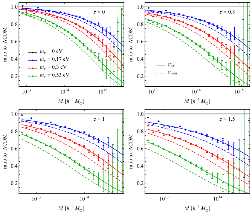 |
We repeat the analysis for Spherical Overdensity (SO) halos, identifying halos as spherical regions with a mean matter density equal to two hundred times the background density, as described in §3. The measurements, shown as ratios to the CDM case, are presented in Figure 11, where now we use the Tinker et al. fitting formula as a reference for SO halos [86]. Also in this case we observe that the Tinker et al. fit, developed in the CDM framework, provides a good fit to simulations with a massive neutrino component when and are used instead of their total dark matter counterparts. Finally, we can assert that a parametrisation of the halo mass function in terms of the CDM power spectrum gives a much better description of measurements from simulations, including massive neutrinos, with respect to the DM power spectrum, both for FoF and SO halos, therefore confirming the results of [25, 26, 93].
6 Halo bias and redshift space distortions
Measurements of the linear bias of FoF halos in massive neutrinos simulations have been presented already in [26], where the authors showed how halo bias at large-scales is scale-independent, as in standard CDM cosmologies, only if defined with respect to the cold, rather than total, matter perturbations. It follows that the halo bias defined with respect to the total matter fluctuations presents a spurious scale-dependence simply arising from the difference between the cold and total matter power spectra, see Fig. 1.
In this section we check, in the first place, these previous results taking advantage of the higher mass resolution of the DEMNUni simulations, with the aim of analysing halo population of sensibly lower mass. In addition, we perform a preliminary analysis of Redshift Space Distortions (RSD) in massive neutrino models with a specific attention to possible consequences of the aforementioned ambiguity in the halo bias definition. More specifically, we test the Kaiser limit [94] of RSD, as the simplest, observable feature of anisotropic galaxy clustering directly dependent on the proper definition of bias. The main goal is to highlight possible systematic effects in the determination of the growth rate, which, in the presence of massive neutrinos, is not simply a function of time, as in CDM models, but presents a mild scale-dependence as well. This analysis is therefore rather complementary to the one of [89] where systematic errors on the determination of RSD parameters induced by neglecting neutrino masses have also been studied.
While we have analysed, for this purpose, three distinct halo populations characterised by distinct mass thresholds, here we focus on the lower one, corresponding to , as less affected by shot-noise and characterised by smaller nonlinear bias corrections. We consider, however, this threshold at different redshifts, presenting the measurements at and as the most relevant for future observations.
6.1 The halo power spectrum in real space
In the local bias approach [95], one can expand the halo overdensity as a power series in , such that on very large scales the bias relation can be written as
| (6.1) |
where the constant is the linear bias factor for the halo population. From the equation above (and from the definition of power spectrum) it follows, in CDM cosmologies, a linear relation between the matter and halo power spectra given by
| (6.2) |
Linear bias can therefore be measured in N-body simulations as in terms of the measured power spectra and . In massive neutrino cosmologies, however, the at the RHS of the above expression can be either the cold or total matter power spectrum, leading to two possible definitions of linear halo (and galaxy) bias, that is
| (6.3) |
or
| (6.4) |
Analogous definitions can be given in terms of the cross halo-matter power spectra, and . The results from §5 and an analogy with CDM cosmologies suggest that bias coefficients are scale-independent only if defined with respect to the cold matter field.
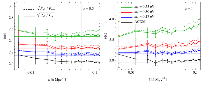
In Figure 12 we present the measurements of halo bias on linear scales from the DEMNUni simulations for halos of masses at redshifts . We consider the bias determined according to both Eq. (6.3) and Eq. (6.4). In all the cases, the bias defined with respect to the total matter perturbations exhibits a larger scale-dependence than the one defined w.r.t. the cold matter component, confirming the findings in [26]. In the rest of the section we will explore possible implications of this fact for the description of RSD at large scales.
6.2 The halo power spectrum in redshift-space
The biasing between the galaxy and matter distributions is not the only effect to be taken into account for a correct estimate of the matter power spectrum from galaxy redshift observations. In a real survey, the proper motions of galaxies with respect to the homogeneous expansion of the Universe affect the determination of their distance along the line-of-sight (see, e.g. [94, 96, 97, 98]). However, on sufficiently large scales these redshift space distortions provide information on the peculiar velocity field of matter perturbations, in particular on the growth rate of the density field, and, as a result, they are extensively used to constrain cosmological parameters and test deviation from standard gravity [99, 100, 101, 102]. In preparation for future large spectroscopic surveys, the effect of neutrino masses on RSD modelling needs to be carefully investigated to avoid fake signatures of Modified Gravity. In the following we present a preliminary assessment of the scale-dependence of the growth rate induced by the free streaming length of neutrinos, and its measurement from the DEMNUni simulations.
In the standard cosmological model, and in the large-scale limit where linear theory applies, the distortion induced by peculiar velocities on the density contrast can be written in Fourier Space as [94]
| (6.5) |
where is the angle between the line-of-sight and the wave vector , while is the linear growth rate, defined as the logarithmic derivative of the linear growth factor , that is
| (6.6) |
A similar expression holds for linearly biased tracers which follow the matter flow (i.e. with no velocity bias888Note that the assumption of no velocity bias is better justified for halos w.r.t. the cold matter perturbations rather than w.r.t. the total matter ones.). For instance, the halo overdensity in redshift space, , can be written as
| (6.7) |
where is the linear scale-independent bias, and we define . It follows that the halo power spectrum in redshift space can be written as the product of a polynomial in times the halo power spectrum in real space. Since the halo power spectrum in real space depends only on the modulus of the wave vector, the angular dependence induced by RSD is entirely encoded in the pre-factor of Eq. (6.7). As a result, the redshift-space halo power spectrum can be decomposed in multipoles using just the first three even Legendre polynomials
| (6.8) |
The monopole, quadrupole and hexadecapole coefficients read
| (6.9) | |||||
| (6.10) | |||||
| (6.11) |
where the RSD parameter determines the relative amplitude of the multipoles. In a CDM cosmology, is predicted to be scale-independent on large scales, as a direct consequence of the scale-independence of both linear bias and growth rate. On the other hand, both quantities might be scale-dependent when massive neutrinos are present.
In the first place, in massive neutrino scenarios, the growth rate of cold matter perturbations, , becomes scale-dependent, as a natural consequence of the scale-dependent growth function . In particular, the small-scale asymptotic suppression expected in linear theory is given by [103]
| (6.12) |
and corresponds to a 2.4% effect for the largest value of the neutrino fraction assumed here, that is in the eV model. However, for the same model, the suppression is below the percent level on large scales, . In the case of the total matter growth rate, , the suppression, again for the eV model, reaches the 1% level at slightly smaller scales, (linear theory predictions for both the ratio and are shown as dashed curves in Figure 14).
In the second place, if we defined the halo bias w.r.t. the total matter field, according to Eq. (6.4), we would add to the quantity an additional source of scale-dependence. Let us notice here that, while one would consider reasonable that the choice of , Eq. (6.3), is consisted with the choice of in the definition of , we cannot exclude a priori other possibilities (including, for instance, a mixed ), since the physical origins of the two contributions in Eq. (6.7) are in fact distinct. However, in what follows, we will limit ourselves to compare the two cases and , the latter corresponding to naïvely neglecting any distinctions between matter contributions.
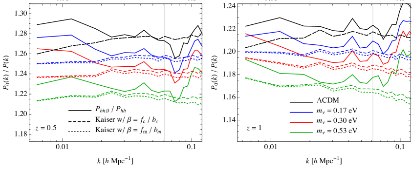
In all the cases, we expect the Kaiser factor to exhibit a scale-dependence, which, by choosing , will result only from the growth rate . In the other case, , a partial compensation occurs between the linear bias, which increases with the wave-number, and the growth factor that actually decreases with . In Figure 13 we show the ratio of the monopole of the redshift-space halo power spectrum, , to the halo power spectrum in real space, , for the models listed in Table 1, and we compare the measurements from the DEMNUni simulations to the corresponding predictions provided by the Kaiser formula written both in terms of and . In such predictions we do not use best fit values for the bias parameters, but we use instead the measured where the scale-dependence is affected by cosmic variance. While the noisy measurements do not allow to clearly determine the scale-independence of such a quantity, we notice that does provide a slightly better prediction than , as compared to simulations.
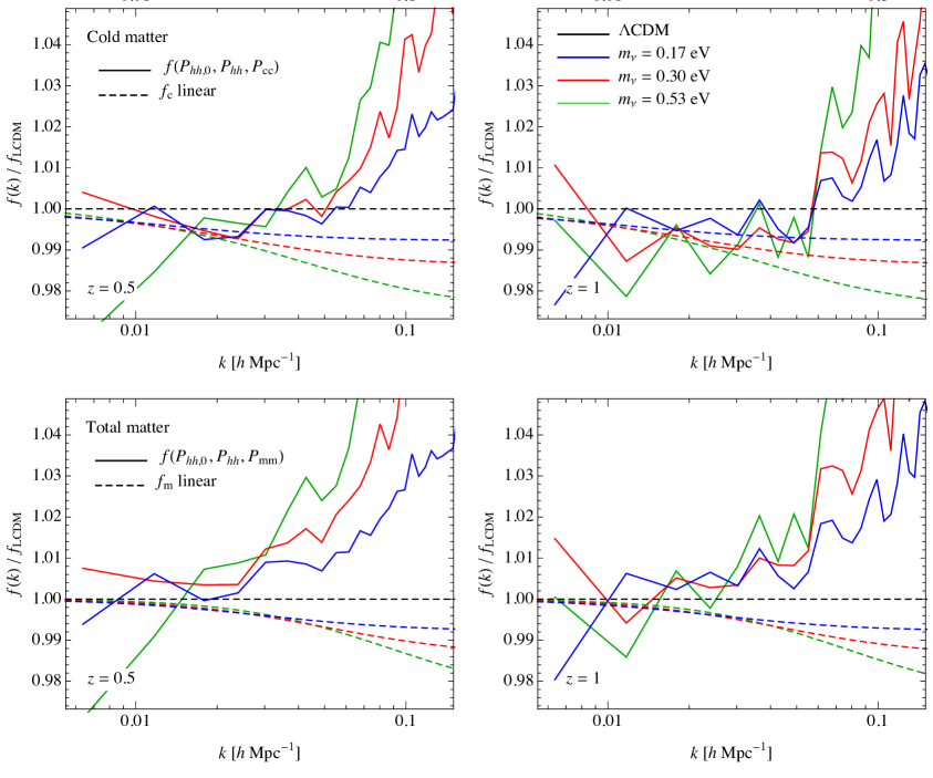
As a further test, in Figure 14 we consider directly the growth rate obtained from measurements of the monopole of the redshift-space halo power spectrum, , and the real-space halo and cold matter power spectra, and respectively, under the assumption that the Kaiser formula provides a good description of RSD at large scales. Assuming , from Eq. (6.9) we have
| (6.13) |
while assuming we obtain a similar expression where replaces . In order to further reduce cosmic variance, we show the recovered value of as ratio to the CDM case. These measurements, as a function of , can then be directly compared with linear theory predictions for and .
The top panels of Figure 14 show obtained from Eq. (6.13) under the cold matter hypothesis compared to the predictions for at redshift . We notice that, in the higher redshift case in particular, despite the noise, the measurements are consistent with the linear predictions at large scales when is obtained from the measured . A greater discrepancy instead is observed when is obtained from the measured total matter , as compared to the predictions for in the bottom panels. If such discrepancy will be confirmed by future investigations, we could expect that using as a definition for bias in the Kaiser formula could lead to a systematic error on the determination of the growth rate at the level of 1-2%.
Clearly this represents a very preliminary analysis of possible systematic effects in the determination of the growth rate in the context of massive neutrinos cosmologies. If the description of halo clustering in terms of cold matter perturbation does indeed represents the correct approach, this test can serve as a confirmation that the DEMNUni simulations reproduce linear theory predictions for the growth rate including, to a certain extent, its scale-dependence. We reserve for future work a more detailed analysis of RSD effects on the matter density field as well as on realistic mock galaxy distributions, in massive neutrino scenarios. Of particular interest would be any description of nonlinearity that could extend theoretical predictions to smaller scales.
7 Conclusions
In this work we have presented an analysis of the LSS clustering features extracted from the DEMNUni simulation suite, a set of large-volume and high-resolution N-body simulations that include massive neutrinos as a particle component. The volume and resolution of these simulations allow the test of several cosmological observables, from the galaxy power spectrum to weak lensing statistics and CMB secondary anisotropies [24]. In this respect, the DEMNUni simulations represent the largest effort to date to include the effects of neutrinos mass in numerical predictions of the large-scale structure. As such, they serve, in the first place, the purpose of investigating our ability to constrain the properties of such important particle for both the standard cosmological model as the standard model of particle physics. At the same time, they can help assessing the effects of massive neutrino on the expected accuracy and precision in the determination of other cosmological parameters, first and foremost those describing possible departures from the CDM paradigm.
We have analysed basic quantities such as the matter power spectrum, the halo mass function, and halo clustering both in real and redshift space, comparing them with the simplest and most common theoretical predictions. This analysis is intended as a first step toward a more accurate test of the latter, taking advantage, however, of recent developments in the understanding of halo formation and clustering.
The most fundamental quantity, in this respect, is the matter power spectrum. In Section 4 we presented measurements of the power spectrum of each individual component of the total matter density, that is the cold dark matter and baryons (here treated on the same footing and called CDM) and the neutrinos, along with their cross-power spectrum and the total matter power spectrum, given by the weighted sum of the three. The analysis in terms of distinct components allows to test early hypothesis regarding the possibility of neglecting the nonlinear evolution of neutrino perturbations in analytical predictions [52]. In this respect we point-out, with direct reference to our measurements, that the neutrino power spectrum, as well as the cross-power spectrum provide a significant contribution to the total matter power spectrum, Eq. (2.5), only at large-scales, where the linear approximation is sufficient. Since the total matter power spectrum, , and the cold matter power spectrum, , are the only quantities directly related to actual observables, a 1% accuracy appears to be achievable even neglecting the nonlinear evolution of neutrino perturbations. With this in mind, we focused on the accurate description of nonlinearity of the cold matter component alone, considering various predictions in perturbation theory, and using, as input quantity, the simple cold matter linear power spectrum. While this is clearly an effective, not rigorous, approach, we have shown that the accuracy provided by PT techniques, and their limits of validity on the matter power spectrum in CDM cosmologies, can be achieved as well for massive neutrino models in a rather simple way. In a completely similar fashion, fitting formulae obtained from CDM simulations, and used beyond the perturbative regime like halofit, can be safely applied to predictions of the nonlinear cold matter power spectrum, and simply extended, with the addition of the linear contributions from the neutrino auto- and CDM-neutrino cross-spectra, to the total matter power spectrum, retaining the same accuracy in presence of massive neutrinos as in a standard massless cosmology, without resorting to additional fitting parameters.
The analysis of the DEMNUni simulations has allowed us to confirm the results of [26, 93] on halo abundances in massive neutrino cosmologies, i.e. that the halo mass function is better described in terms of the variance of cold matter fluctuations alone. Similarly, from the study of halo clustering, we have confirmed as well that a constant linear, halo bias is recovered in the large-scale limit only when the bias relation is considered between halo and cold (rather than total) matter distributions. Such peculiar ambiguity in the definition of halo (and galaxy) bias, motivated a preliminary test of the Kaiser formula for redshift-space distortions [94], where linear bias is a relevant parameter. We found, despite the yet large statistical uncertainty, some indications of the expected scale-dependence of the growth rate of matter perturbation, characteristic of massive neutrino cosmologies. If such indications are correct, then we have shown that defining the galaxy bias w.r.t. the cold matter component is necessary to avoid a systematic error on the determination of the growth rate at the few percent level. We will return on the subject in more detail in future work.
Acknowledgements
We thank Jason Dossett, Carlo Schimd, Roman Scoccimarro for useful discussions. We are especially grateful for the support of Margarita Petkova through the Computational Center for Particle and Astrophysics (C2PAP). We are also particularly grateful to Francisco Villaescusa-Navarro for making available to us the results of his simulations used in Fig. 8, and for a constant exchange of ideas during the development of the results presented in this paper. C.C. and K.D. thank Matteo Viel for providing the N-GenIC code for initial conditions, modified to take into account a massive neutrino particle component. The DEMNUni simulations were carried out at the Tier-0 IBM BG/Q machine, Fermi, of the Centro Interuniversitario del Nord-Est per il Calcolo Elettronico (CINECA, Bologna, Italy), via the five million cpu-hrs budget provided by the Italian SuperComputing Resource Allocation (ISCRA) to the class–A proposal entitled “The Dark-Energy and Massive-Neutrino Universe”. C.C. is extremely grateful to CINECA system managers for the great help and support provided during the simulation production at Fermi, and the “BigData” management and storage, via the new computing system PICO, which drives a large data repository shared among all the HPC systems at CINECA. C.C. thanks Federico Marulli, Lauro Moscardini, and Andrea Cimatti for useful discussions in the preparation of the DEMNUni proposal. C.C. acknowledges financial support from the INAF Fellowships Programme 2010. K.D. acknowledges the support by the DFG Cluster of Excellence “Origin and Structure of the Universe”. E.S. would like to express as well his gratitude to Ivan Girotto at ICTP for his invaluable kindness and technical help in the solution of issues related to the data analysis presented in this paper. E.S. acknowledges financial contribution from contracts ASI/INAF n.I/023/12/0 ‘Attivià relative alla fase B2/C per la missione Euclid. J.B. and C.C. also acknowledge financial support from the European Research Council through the Darklight Advanced Research Grant (n. 291521).
References
- [1] Y. Fukuda, T. Hayakawa, E. Ichihara, K. Inoue, K. Ishihara, H. Ishino, Y. Itow, T. Kajita, J. Kameda, S. Kasuga, K. Kobayashi, Y. Kobayashi, Y. Koshio, M. Miura, M. Nakahata, S. Nakayama, A. Okada, K. Okumura, N. Sakurai, M. Shiozawa, Y. Suzuki, Y. Takeuchi, Y. Totsuka, S. Yamada, M. Earl, A. Habig, E. Kearns, M. D. Messier, K. Scholberg, J. L. Stone, L. R. Sulak, C. W. Walter, M. Goldhaber, T. Barszczxak, D. Casper, W. Gajewski, P. G. Halverson, J. Hsu, W. R. Kropp, L. R. Price, F. Reines, M. Smy, H. W. Sobel, M. R. Vagins, K. S. Ganezer, W. E. Keig, R. W. Ellsworth, S. Tasaka, J. W. Flanagan, A. Kibayashi, J. G. Learned, S. Matsuno, V. J. Stenger, D. Takemori, T. Ishii, J. Kanzaki, T. Kobayashi, S. Mine, K. Nakamura, K. Nishikawa, Y. Oyama, A. Sakai, M. Sakuda, O. Sasaki, S. Echigo, M. Kohama, A. T. Suzuki, T. J. Haines, E. Blaufuss, B. K. Kim, R. Sanford, R. Svoboda, M. L. Chen, Z. Conner, J. A. Goodman, G. W. Sullivan, J. Hill, C. K. Jung, K. Martens, C. Mauger, C. McGrew, E. Sharkey, B. Viren, C. Yanagisawa, W. Doki, K. Miyano, H. Okazawa, C. Saji, M. Takahata, Y. Nagashima, M. Takita, T. Yamaguchi, M. Yoshida, S. B. Kim, M. Etoh, K. Fujita, A. Hasegawa, T. Hasegawa, S. Hatakeyama, T. Iwamoto, M. Koga, T. Maruyama, H. Ogawa, J. Shirai, A. Suzuki, F. Tsushima, M. Koshiba, M. Nemoto, K. Nishijima, T. Futagami, Y. Hayato, Y. Kanaya, K. Kaneyuki, Y. Watanabe, D. Kielczewska, R. A. Doyle, J. S. George, A. L. Stachyra, L. L. Wai, R. J. Wilkes, and K. K. Young, Evidence for Oscillation of Atmospheric Neutrinos, Physical Review Letters 81 1562–1567, [hep-ex/9807003].
- [2] G. L. Fogli, E. Lisi, A. Marrone, D. Montanino, A. Palazzo, and A. M. Rotunno, Global analysis of neutrino masses, mixings, and phases: Entering the era of leptonic CP violation searches, Phys. Rev. D 86 013012, [arXiv:1205.5254].
- [3] D. V. Forero, M. Tórtola, and J. W. F. Valle, Global status of neutrino oscillation parameters after Neutrino-2012, Phys. Rev. D 86 073012, [arXiv:1205.4018].
- [4] J. Lesgourgues and S. Pastor, Massive neutrinos and cosmology, Phys. Rep. 429 307–379, [astro-ph/0603494].
- [5] J. Lesgourgues, G. Mangano, G. Miele, and S. Pastor, Neutrino Cosmology. Cambridge, UK: Cambridge University Press, Feb., 2013.
- [6] S. Hannestad, Neutrino masses and the number of neutrino species from WMAP and 2dFGRS, Journal of Cosmology and Astro-Particle Physics 5 4, [astro-ph/0303076].
- [7] B. A. Reid, L. Verde, R. Jimenez, and O. Mena, Robust neutrino constraints by combining low redshift observations with the CMB, Journal of Cosmology and Astro-Particle Physics 1 3, [arXiv:0910.0008].
- [8] S. A. Thomas, F. B. Abdalla, and O. Lahav, Upper Bound of 0.28 eV on Neutrino Masses from the Largest Photometric Redshift Survey, Physical Review Letters 105 031301, [arXiv:0911.5291].
- [9] M. E. C. Swanson, W. J. Percival, and O. Lahav, Neutrino masses from clustering of red and blue galaxies: a test of astrophysical uncertainties, Mon. Not. R. Astron. Soc. 409 1100–1112, [arXiv:1006.2825].
- [10] S. Saito, M. Takada, and A. Taruya, Neutrino mass constraint from the Sloan Digital Sky Survey power spectrum of luminous red galaxies and perturbation theory, Phys. Rev. D 83 043529, [arXiv:1006.4845].
- [11] C. Carbone, L. Verde, Y. Wang, and A. Cimatti, Neutrino constraints from future nearly all-sky spectroscopic galaxy surveys, Journal of Cosmology and Astro-Particle Physics 3 30, [arXiv:1012.2868].
- [12] R. de Putter, O. Mena, E. Giusarma, S. Ho, A. Cuesta, H.-J. Seo, A. J. Ross, M. White, D. Bizyaev, H. Brewington, D. Kirkby, E. Malanushenko, V. Malanushenko, D. Oravetz, K. Pan, W. J. Percival, N. P. Ross, D. P. Schneider, A. Shelden, A. Simmons, and S. Snedden, New Neutrino Mass Bounds from SDSS-III Data Release 8 Photometric Luminous Galaxies, Astrophys. J. 761 12, [arXiv:1201.1909].
- [13] J.-Q. Xia, B. R. Granett, M. Viel, S. Bird, L. Guzzo, M. G. Haehnelt, J. Coupon, H. J. McCracken, and Y. Mellier, Constraints on massive neutrinos from the CFHTLS angular power spectrum, Journal of Cosmology and Astro-Particle Physics 6 10, [arXiv:1203.5105].
- [14] S. Riemer-Sørensen, C. Blake, D. Parkinson, T. M. Davis, S. Brough, M. Colless, C. Contreras, W. Couch, S. Croom, D. Croton, M. J. Drinkwater, K. Forster, D. Gilbank, M. Gladders, K. Glazebrook, B. Jelliffe, R. J. Jurek, I.-h. Li, B. Madore, D. C. Martin, K. Pimbblet, G. B. Poole, M. Pracy, R. Sharp, E. Wisnioski, D. Woods, T. K. Wyder, and H. K. C. Yee, WiggleZ Dark Energy Survey: Cosmological neutrino mass constraint from blue high-redshift galaxies, Phys. Rev. D 85 081101, [arXiv:1112.4940].
- [15] G.-B. Zhao, S. Saito, W. J. Percival, A. J. Ross, F. Montesano, M. Viel, D. P. Schneider, M. Manera, J. Miralda-Escudé, N. Palanque-Delabrouille, N. P. Ross, L. Samushia, A. G. Sánchez, M. E. C. Swanson, D. Thomas, R. Tojeiro, C. Yèche, and D. G. York, The clustering of galaxies in the SDSS-III Baryon Oscillation Spectroscopic Survey: weighing the neutrino mass using the galaxy power spectrum of the CMASS sample, Mon. Not. R. Astron. Soc. [arXiv:1211.3741].
- [16] S. More, F. C. van den Bosch, M. Cacciato, A. More, H. Mo, and X. Yang, Cosmological constraints from a combination of galaxy clustering and lensing - II. Fisher matrix analysis, Mon. Not. R. Astron. Soc. 430 747–766, [arXiv:1207.0004].
- [17] E. Giusarma, R. de Putter, S. Ho, and O. Mena, Constraints on neutrino masses from Planck and Galaxy clustering data, Phys. Rev. D 88 063515, [arXiv:1306.5544].
- [18] M. Wyman, D. H. Rudd, R. A. Vanderveld, and W. Hu, nu-LCDM: Neutrinos reconcile Planck with the Local Universe, ArXiv e-prints [arXiv:1307.7715].
- [19] R. A. Battye and A. Moss, Evidence for Massive Neutrinos from Cosmic Microwave Background and Lensing Observations, Physical Review Letters 112 051303, [arXiv:1308.5870].
- [20] S. Riemer-Sørensen, D. Parkinson, and T. M. Davis, Combining Planck data with large scale structure information gives a strong neutrino mass constraint, Phys. Rev. D 89 103505, [arXiv:1306.4153].
- [21] F. Beutler, S. Saito, J. R. Brownstein, C.-H. Chuang, A. J. Cuesta, W. J. Percival, A. J. Ross, N. P. Ross, D. P. Schneider, L. Samushia, A. G. Sánchez, H.-J. Seo, J. L. Tinker, C. Wagner, and B. A. Weaver, The clustering of galaxies in the SDSS-III Baryon Oscillation Spectroscopic Survey: signs of neutrino mass in current cosmological data sets, Mon. Not. R. Astron. Soc. 444 3501–3516, [arXiv:1403.4599].
- [22] K. N. Abazajian, K. Arnold, J. Austermann, B. A. Benson, C. Bischoff, J. Bock, J. R. Bond, J. Borrill, E. Calabrese, J. E. Carlstrom, C. S. Carvalho, C. L. Chang, H. C. Chiang, S. Church, A. Cooray, T. M. Crawford, K. S. Dawson, S. Das, M. J. Devlin, M. Dobbs, S. Dodelson, O. Doré, J. Dunkley, J. Errard, A. Fraisse, J. Gallicchio, N. W. Halverson, S. Hanany, S. R. Hildebrandt, A. Hincks, R. Hlozek, G. Holder, W. L. Holzapfel, K. Honscheid, W. Hu, J. Hubmayr, K. Irwin, W. C. Jones, M. Kamionkowski, B. Keating, R. Keisler, L. Knox, E. Komatsu, J. Kovac, C.-L. Kuo, C. Lawrence, A. T. Lee, E. Leitch, E. Linder, P. Lubin, J. McMahon, A. Miller, L. Newburgh, M. D. Niemack, H. Nguyen, H. T. Nguyen, L. Page, C. Pryke, C. L. Reichardt, J. E. Ruhl, N. Sehgal, U. Seljak, J. Sievers, E. Silverstein, A. Slosar, K. M. Smith, D. Spergel, S. T. Staggs, A. Stark, R. Stompor, A. G. Vieregg, G. Wang, S. Watson, E. J. Wollack, W. L. K. Wu, K. W. Yoon, and O. Zahn, Neutrino physics from the cosmic microwave background and large scale structure, Astroparticle Physics 63 66–80.
- [23] H. Böhringer and G. Chon, The extended ROSAT-ESO Flux-Limited X-ray Galaxy Cluster Survey (REFLEX II). VI. Effect of massive neutrinos on the cosmological constraints from clusters, Astron. Astrophys. 574 L8, [arXiv:1501.0495].
- [24] C. Carbone, M. Petkova, and K. Dolag in preparation.
- [25] K. Ichiki and M. Takada, Impact of massive neutrinos on the abundance of massive clusters, Phys. Rev. D 85 063521, [arXiv:1108.4688].
- [26] E. Castorina, E. Sefusatti, R. K. Sheth, F. Villaescusa-Navarro, and M. Viel, Cosmology with massive neutrinos II: on the universality of the halo mass function and bias, Journal of Cosmology and Astro-Particle Physics 2 49, [arXiv:1311.1212].
- [27] D. Blas, M. Garny, T. Konstandin, and J. Lesgourgues, Structure formation with massive neutrinos: going beyond linear theory, Journal of Cosmology and Astro-Particle Physics 11 39, [arXiv:1408.2995].
- [28] R. E. Smith, J. A. Peacock, A. Jenkins, S. D. M. White, C. S. Frenk, F. R. Pearce, P. A. Thomas, G. Efstathiou, and H. M. P. Couchman, Stable clustering, the halo model and non-linear cosmological power spectra, Mon. Not. R. Astron. Soc. 341 1311–1332, [astro-ph/0207664].
- [29] S. Bird, M. Viel, and M. G. Haehnelt, Massive neutrinos and the non-linear matter power spectrum, Mon. Not. R. Astron. Soc. 420 2551–2561, [arXiv:1109.4416].
- [30] R. Takahashi, M. Sato, T. Nishimichi, A. Taruya, and M. Oguri, Revising the Halofit Model for the Nonlinear Matter Power Spectrum, Astrophys. J. 761 152, [arXiv:1208.2701].
- [31] R. Ruggieri, E. Castorina, E. Sefusatti, and C. Carbone in preparation.
- [32] M. Costanzi, B. Sartoris, M. Viel, and S. Borgani, Neutrino constraints: what large-scale structure and CMB data are telling us?, Journal of Cosmology and Astro-Particle Physics 10 81, [arXiv:1407.8338].
- [33] Planck Collaboration, P. A. R. Ade, N. Aghanim, M. Arnaud, M. Ashdown, J. Aumont, C. Baccigalupi, A. J. Banday, R. B. Barreiro, J. G. Bartlett, and et al., Planck 2015 results. XXIV. Cosmology from Sunyaev-Zeldovich cluster counts, ArXiv e-prints [arXiv:1502.0159].
- [34] M. Takada, E. Komatsu, and T. Futamase, Cosmology with high-redshift galaxy survey: Neutrino mass and inflation, Phys. Rev. D 73 083520, [astro-ph/0512374].
- [35] G. Mangano, G. Miele, S. Pastor, T. Pinto, O. Pisanti, and P. D. Serpico, Relic neutrino decoupling including flavour oscillations, Nuclear Physics B 729 221–234, [hep-ph/0506164].
- [36] W. Hu, D. J. Eisenstein, and M. Tegmark, Weighing Neutrinos with Galaxy Surveys, Physical Review Letters 80 5255–5258, [astro-ph/9712057].
- [37] V. Springel, The cosmological simulation code GADGET-2, Mon. Not. R. Astron. Soc. 364 1105–1134, [astro-ph/0505010].
- [38] M. Viel, M. G. Haehnelt, and V. Springel, The effect of neutrinos on the matter distribution as probed by the intergalactic medium, Journal of Cosmology and Astro-Particle Physics 6 15, [arXiv:1003.2422].
- [39] F. Villaescusa-Navarro, S. Bird, C. Peña-Garay, and M. Viel, Non-linear evolution of the cosmic neutrino background, Journal of Cosmology and Astro-Particle Physics 3 19, [arXiv:1212.4855].
- [40] S. Bird, M. Viel, and M. G. Haehnelt, Massive neutrinos and the non-linear matter power spectrum, Mon. Not. R. Astron. Soc. 420 2551–2561, [arXiv:1109.4416].
- [41] P. A. R. Ade, N. Aghanim, C. Armitage-Caplan, M. Arnaud, M. Ashdown, F. Atrio-Barandela, J. Aumont, C. Baccigalupi, A. J. Banday, and et al., Planck 2013 results. XVI. Cosmological parameters, ArXiv e-prints [arXiv:1303.5076].
- [42] V. Springel, N. Yoshida, and S. D. M. White, GADGET: a code for collisionless and gasdynamical cosmological simulations, New Astronomy 6 79–117, [astro-ph/0003162].
- [43] K. Dolag, S. Borgani, G. Murante, and V. Springel, Substructures in hydrodynamical cluster simulations, Mon. Not. R. Astron. Soc. 399 497–514, [arXiv:0808.3401].
- [44] J. Brandbyge, S. Hannestad, T. Haugbølle, and Y. Y. Y. Wong, Neutrinos in non-linear structure formation - the effect on halo properties, Journal of Cosmology and Astro-Particle Physics 9 14, [arXiv:1004.4105].
- [45] R. E. Smith, J. A. Peacock, A. Jenkins, S. D. M. White, C. S. Frenk, F. R. Pearce, P. A. Thomas, G. Efstathiou, and H. M. P. Couchman, Stable clustering, the halo model and non-linear cosmological power spectra, Mon. Not. R. Astron. Soc. 341 1311–1332, [astro-ph/0207664].
- [46] D. H. Rudd, A. R. Zentner, and A. V. Kravtsov, Effects of Baryons and Dissipation on the Matter Power Spectrum, Astrophys. J. 672 19–32, [astro-ph/].
- [47] T. Guillet, R. Teyssier, and S. Colombi, The effect of baryons on the variance and the skewness of the mass distribution in the Universe at small scales, Mon. Not. R. Astron. Soc. 405 525–534, [arXiv:0905.2615].
- [48] L. Casarini, A. V. Macciò, S. A. Bonometto, and G. S. Stinson, High-accuracy power spectra including baryonic physics in dynamical Dark Energy models, Mon. Not. R. Astron. Soc. 412 911–920, [arXiv:1005.4683].
- [49] M. P. van Daalen, J. Schaye, C. M. Booth, and C. Dalla Vecchia, The effects of galaxy formation on the matter power spectrum: a challenge for precision cosmology, Mon. Not. R. Astron. Soc. 415 3649–3665, [arXiv:1104.1174].
- [50] M. P. van Daalen, J. Schaye, I. G. McCarthy, C. M. Booth, and C. Dalla Vecchia, The impact of baryonic processes on the two-point correlation functions of galaxies, subhaloes and matter, ArXiv e-prints [arXiv:1310.7571].
- [51] J. Bel, M. Zennaro, F. Villaescusa-Navarro, E. Sefusatti, and C. Carbone in preparation.
- [52] S. Saito, M. Takada, and A. Taruya, Impact of Massive Neutrinos on the Nonlinear Matter Power Spectrum, Physical Review Letters 100 191301, [arXiv:0801.0607].
- [53] Y. Y. Y. Wong, Higher order corrections to the large scale matter power spectrum in the presence of massive neutrinos, Journal of Cosmology and Astro-Particle Physics 10 35, [arXiv:0809.0693].
- [54] S. Saito, M. Takada, and A. Taruya, Nonlinear power spectrum in the presence of massive neutrinos: Perturbation theory approach, galaxy bias, and parameter forecasts, Phys. Rev. D 80 083528, [arXiv:0907.2922].
- [55] J. Lesgourgues, S. Matarrese, M. Pietroni, and A. Riotto, Non-linear power spectrum including massive neutrinos: the time-rg flow approach, Journal of Cosmology and Astro-Particle Physics 6 17, [ 0901.455].
- [56] M. Shoji and E. Komatsu, Third-order perturbation theory with nonlinear pressure, Astrophys. J. 700 705–719, [arXiv:0903.2669].
- [57] M. Shoji and E. Komatsu, Massive neutrinos in cosmology: Analytic solutions and fluid approximation, Phys. Rev. D 81 123516.
- [58] F. Führer and Y. Y. Y. Wong, Higher-order massive neutrino perturbations in large-scale structure, Journal of Cosmology and Astro-Particle Physics 3 46, [arXiv:1412.2764].
- [59] H. Dupuy and F. Bernardeau, Describing massive neutrinos in cosmology as a collection of independent flows, Journal of Cosmology and Astro-Particle Physics 1 30, [arXiv:1311.5487].
- [60] H. Dupuy and F. Bernardeau, On the importance of nonlinear couplings in large-scale neutrino streams, ArXiv e-prints [arXiv:1503.0570].
- [61] F. Bernardeau, M. Crocce, and R. Scoccimarro, Multipoint propagators in cosmological gravitational instability, Phys. Rev. D 78 103521, [arXiv:0806.2334].
- [62] A. Taruya, F. Bernardeau, T. Nishimichi, and S. Codis, Direct and fast calculation of regularized cosmological power spectrum at two-loop order, Phys. Rev. D 86 103528, [arXiv:1208.1191].
- [63] A. Schneider, R. Teyssier, D. Potter, J. Stadel, J. Onions, D. S. Reed, R. E. Smith, V. Springel, and F. R. Pearce, Matter power spectrum and the challenge of percent accuracy, ArXiv e-prints [arXiv:1503.0592].
- [64] D. Blas, M. Garny, and T. Konstandin, Cosmological perturbation theory at three-loop order, Journal of Cosmology and Astro-Particle Physics 1 10, [arXiv:1309.3308].
- [65] P. Fosalba, M. Crocce, E. Gaztañaga, and F. J. Castander, The MICE Grand Challenge Lightcone Simulation I: Dark matter clustering, ArXiv e-prints [arXiv:1312.1707].
- [66] A. Upadhye, R. Biswas, A. Pope, K. Heitmann, S. Habib, H. Finkel, and N. Frontiere, Large-scale structure formation with massive neutrinos and dynamical dark energy, Phys. Rev. D 89 103515, [arXiv:1309.5872].
- [67] M. Pietroni, Flowing with time: a new approach to non-linear cosmological perturbations, Journal of Cosmology and Astro-Particle Physics 10 36, [arXiv:0806.0971].
- [68] A. J. S. Hamilton, P. Kumar, E. Lu, and A. Matthews, Reconstructing the primordial spectrum of fluctuations of the universe from the observed nonlinear clustering of galaxies, Astrophys. J. Lett. 374 L1–L4.
- [69] J. A. Peacock and S. J. Dodds, Reconstructing the Linear Power Spectrum of Cosmological Mass Fluctuations, Mon. Not. R. Astron. Soc. 267 1020, [astro-ph/9311057].
- [70] A. Lewis, A. Challinor, and A. Lasenby, Efficient computation of cosmic microwave background anisotropies in closed friedmann-robertson-walker models, Astrophys. J. 538 473–476, [astro-ph/9911177].
- [71] J. Lesgourgues, The Cosmic Linear Anisotropy Solving System (CLASS) I: Overview, ArXiv e-prints [arXiv:1104.2932].
- [72] F. Villaescusa-Navarro, F. Marulli, M. Viel, E. Branchini, E. Castorina, E. Sefusatti, and S. Saito, Cosmology with massive neutrinos I: towards a realistic modeling of the relation between matter, haloes and galaxies, Journal of Cosmology and Astro-Particle Physics 3 11, [arXiv:1311.0866].
- [73] E. Massara, F. Villaescusa-Navarro, and M. Viel, The halo model in a massive neutrino cosmology, Journal of Cosmology and Astro-Particle Physics 12 53, [arXiv:1410.6813].
- [74] S. Wang, Z. Haiman, W. Hu, J. Khoury, and M. May, Weighing Neutrinos with Galaxy Cluster Surveys, Physical Review Letters 95 011302, [astro-ph/0505390].
- [75] A. Mantz, S. W. Allen, and D. Rapetti, The observed growth of massive galaxy clusters - IV. Robust constraints on neutrino properties, Mon. Not. R. Astron. Soc. 406 1805–1814, [arXiv:0911.1788].
- [76] C. Carbone, C. Fedeli, L. Moscardini, and A. Cimatti, Measuring the neutrino mass from future wide galaxy cluster catalogues, Journal of Cosmology and Astro-Particle Physics 3 23, [arXiv:1112.4810].
- [77] Planck Collaboration, P. A. R. Ade, N. Aghanim, M. Arnaud, M. Ashdown, J. Aumont, C. Baccigalupi, A. J. Banday, R. B. Barreiro, J. G. Bartlett, and et al., Planck 2015 results. XIII. Cosmological parameters, ArXiv e-prints [arXiv:1502.0158].
- [78] R. A. Battye, T. Charnock, and A. Moss, Tension between the power spectrum of density perturbations measured on large and small scales, ArXiv e-prints [arXiv:1409.2769].
- [79] B. Leistedt, H. V. Peiris, and L. Verde, No New Cosmological Concordance with Massive Sterile Neutrinos, Physical Review Letters 113 041301, [arXiv:1404.5950].
- [80] A. B. Mantz, A. von der Linden, S. W. Allen, D. E. Applegate, P. L. Kelly, R. G. Morris, D. A. Rapetti, R. W. Schmidt, S. Adhikari, M. T. Allen, P. R. Burchat, D. L. Burke, M. Cataneo, D. Donovan, H. Ebeling, S. Shandera, and A. Wright, Weighing the giants - IV. Cosmology and neutrino mass, Mon. Not. R. Astron. Soc. 446 2205–2225, [arXiv:1407.4516].
- [81] M. Roncarelli, C. Carbone, and L. Moscardini, The effect of massive neutrinos on the Sunyaev-Zel’dovich and X-ray observables of galaxy clusters, Mon. Not. R. Astron. Soc. 447 1761–1773, [arXiv:1409.4285].
- [82] M. S. Warren, K. Abazajian, D. E. Holz, and L. Teodoro, Precision Determination of the Mass Function of Dark Matter Halos, Astrophys. J. 646 881–885, [astro-ph/0506395].
- [83] W. H. Press and P. Schechter, Formation of Galaxies and Clusters of Galaxies by Self-Similar Gravitational Condensation, Astrophys. J. 187 425–438.
- [84] M. Musso and R. K. Sheth, One step beyond: the excursion set approach with correlated steps, Mon. Not. R. Astron. Soc. 423 L102–L106, [arXiv:1201.3876].
- [85] A. Paranjape, R. K. Sheth, and V. Desjacques, Excursion set peaks: a self-consistent model of dark halo abundances and clustering, Mon. Not. R. Astron. Soc. 431 1503–1512, [arXiv:1210.1483].
- [86] J. Tinker, A. V. Kravtsov, A. A. Klypin, K. Abazajian, M. S. Warren, G. Yepes, S. Gottlöber, and D. E. Holz, Toward a Halo Mass Function for Precision Cosmology: The Limits of Universality, Astrophys. J. 688 709–728, [arXiv:0803.2706].
- [87] M. Crocce, P. Fosalba, F. J. Castander, and E. Gaztañaga, Simulating the Universe with MICE: the abundance of massive clusters, Mon. Not. R. Astron. Soc. 403 1353–1367, [arXiv:0907.0019].
- [88] W. A. Watson, I. T. Iliev, A. D’Aloisio, A. Knebe, P. R. Shapiro, and G. Yepes, The halo mass function through the cosmic ages, Mon. Not. R. Astron. Soc. [arXiv:1212.0095].
- [89] F. Marulli, C. Carbone, M. Viel, L. Moscardini, and A. Cimatti, Effects of massive neutrinos on the large-scale structure of the Universe, Mon. Not. R. Astron. Soc. 418 346–356, [arXiv:1103.0278].
- [90] M. LoVerde and M. Zaldarriaga, Neutrino clustering around spherical dark matter halos, Phys. Rev. D 89 063502, [arXiv:1310.6459].
- [91] M. LoVerde, Spherical collapse in CDM, Phys. Rev. D 90 083518, [arXiv:1405.4858].
- [92] M. Costanzi, F. Villaescusa-Navarro, M. Viel, J.-Q. Xia, S. Borgani, E. Castorina, and E. Sefusatti, Cosmology with massive neutrinos III: the halo mass function and an application to galaxy clusters, Journal of Cosmology and Astro-Particle Physics 12 12, [arXiv:1311.1514].
- [93] M. Costanzi Alunno Cerbolini, B. Sartoris, J.-Q. Xia, A. Biviano, S. Borgani, and M. Viel, Constraining neutrino properties with a Euclid-like galaxy cluster survey, ArXiv e-prints [arXiv:1303.4550].
- [94] N. Kaiser, Clustering in real space and in redshift space, Mon. Not. R. Astron. Soc. 227 1–21.
- [95] J. N. Fry and E. Gaztañaga, Biasing and hierarchical statistics in large-scale structure, Astrophys. J. 413 447–452, [astro-ph/9302009].
- [96] R. Scoccimarro, Redshift-space distortions, pairwise velocities, and nonlinearities, Phys. Rev. D 70 083007–+, [astro-ph/].
- [97] B. A. Reid and M. White, Towards an accurate model of the redshift-space clustering of haloes in the quasi-linear regime, Mon. Not. R. Astron. Soc. 417 1913–1927, [arXiv:1105.4165].
- [98] D. Bianchi, M. Chiesa, and L. Guzzo, Improving the modelling of redshift-space distortions - I. A bivariate Gaussian description for the galaxy pairwise velocity distributions, Mon. Not. R. Astron. Soc. 446 75–84, [arXiv:1407.4753].
- [99] L. Guzzo, M. Pierleoni, B. Meneux, E. Branchini, O. Le Fèvre, C. Marinoni, B. Garilli, J. Blaizot, G. De Lucia, A. Pollo, H. J. McCracken, D. Bottini, V. Le Brun, D. Maccagni, J. P. Picat, R. Scaramella, M. Scodeggio, L. Tresse, G. Vettolani, A. Zanichelli, C. Adami, S. Arnouts, S. Bardelli, M. Bolzonella, A. Bongiorno, A. Cappi, S. Charlot, P. Ciliegi, T. Contini, O. Cucciati, S. de la Torre, K. Dolag, S. Foucaud, P. Franzetti, I. Gavignaud, O. Ilbert, A. Iovino, F. Lamareille, B. Marano, A. Mazure, P. Memeo, R. Merighi, L. Moscardini, S. Paltani, R. Pellò, E. Perez-Montero, L. Pozzetti, M. Radovich, D. Vergani, G. Zamorani, and E. Zucca, A test of the nature of cosmic acceleration using galaxy redshift distortions, Nature 451 541–544, [arXiv:0802.1944].
- [100] S. de la Torre, L. Guzzo, J. A. Peacock, E. Branchini, A. Iovino, B. R. Granett, U. Abbas, C. Adami, S. Arnouts, J. Bel, M. Bolzonella, D. Bottini, A. Cappi, J. Coupon, O. Cucciati, I. Davidzon, G. De Lucia, A. Fritz, P. Franzetti, M. Fumana, B. Garilli, O. Ilbert, J. Krywult, V. Le Brun, O. Le Fevre, D. Maccagni, K. Malek, F. Marulli, H. J. McCracken, L. Moscardini, L. Paioro, W. J. Percival, M. Polletta, A. Pollo, H. Schlagenhaufer, M. Scodeggio, L. A. M. Tasca, R. Tojeiro, D. Vergani, A. Zanichelli, A. Burden, C. Di Porto, A. Marchetti, C. Marinoni, Y. Mellier, P. Monaco, R. C. Nichol, S. Phleps, M. Wolk, and G. Zamorani, The VIMOS Public Extragalactic Redshift Survey (VIPERS). Galaxy clustering and redshift-space distortions at z=0.8 in the first data release, ArXiv e-prints [arXiv:1303.2622].
- [101] C. Contreras, C. Blake, G. B. Poole, F. Marin, S. Brough, M. Colless, W. Couch, S. Croom, D. Croton, T. M. Davis, M. J. Drinkwater, K. Forster, D. Gilbank, M. Gladders, K. Glazebrook, B. Jelliffe, R. J. Jurek, I.-h. Li, B. Madore, D. C. Martin, K. Pimbblet, M. Pracy, R. Sharp, E. Wisnioski, D. Woods, T. K. Wyder, and H. K. C. Yee, The WiggleZ Dark Energy Survey: measuring the cosmic growth rate with the two-point galaxy correlation function, Mon. Not. R. Astron. Soc. 430 924–933, [arXiv:1302.5178].
- [102] F. Beutler, S. Saito, H.-J. Seo, J. Brinkmann, K. S. Dawson, D. J. Eisenstein, A. Font-Ribera, S. Ho, C. K. McBride, F. Montesano, W. J. Percival, A. J. Ross, N. P. Ross, L. Samushia, D. J. Schlegel, A. G. Sánchez, J. L. Tinker, and B. A. Weaver, The clustering of galaxies in the SDSS-III Baryon Oscillation Spectroscopic Survey: testing gravity with redshift space distortions using the power spectrum multipoles, Mon. Not. R. Astron. Soc. 443 1065–1089, [arXiv:1312.4611].
- [103] J. R. Bond, G. P. Efstathiou, and J. Silk, Massive neutrinos and the large-scale structure of the universe, Physical Review Letters 45 1980–1984.