Galaxies in CDM with Halo Abundance Matching: luminosity-velocity relation, baryonic mass-velocity relation, velocity function and clustering
APPENDIX
Abstract
It has long been regarded as difficult if not impossible for a cosmological model to account simultaneously for the galaxy luminosity, mass, and velocity distributions. We revisit this issue using a modern compilation of observational data along with the best available large-scale cosmological simulation of dark matter. We find that the standard cosmological model, used in conjunction with halo abundance matching (HAM) and simple dynamical corrections, fits – at least on average – all basic statistics of galaxies with circular velocities calculated at a radius of 10 kpc. Our primary observational constraint is the luminosity-velocity relation – which generalizes the Tully-Fisher and Faber-Jackson relations in allowing all types of galaxies to be included, and provides a fundamental benchmark to be reproduced by any theory of galaxy formation. We have compiled data for a variety of galaxies ranging from dwarf irregulars to giant ellipticals. The data present a clear monotonic luminosity-velocity relation from 50 km s-1 to 500 km s-1, with a bend below 80 km s-1 and a systematic offset between late- and early-type galaxies. For comparison to theory, we employ our new CDM “Bolshoi” simulation of dark matter, which has unprecedented mass and force resolution over a large cosmological volume, while using an up-to-date set of cosmological parameters. We use halo abundance matching to assign rank-ordered galaxy luminosities to the dark matter halos, a procedure that automatically fits the empirical luminosity function and provides a predicted luminosity-velocity relation that can be checked against observations. The adiabatic contraction of dark matter halos in response to the infall of the baryons is included as an optional model ingredient. The resulting predictions for the luminosity-velocity relation are in excellent agreement with the available data on both early-type and late-type galaxies for the luminosity range from to . We also compare our predictions for the “cold” baryon mass (i.e., stars and cold gas) of galaxies as a function of circular velocity with the available observations, again finding a very good agreement. The predicted circular velocity function is also in agreement with the galaxy velocity function from 80 to 400 km s-1, using the HIPASS survey for late-type and SDSS for early-type galaxies. However, in accord with other recent results, we find that the dark matter halos with are much more abundant than observed galaxies with the same . Finally, we find that the two-point correlation function of bright galaxies in our model matches very well the results from the final data release of the SDSS, especially when a small amount of scatter is included in the HAM prescription.
1 Introduction
The cosmological constant + cold dark matter (CDM) model is the reigning paradigm of structure formation in the universe. The presence of large amounts of dark mass in the surroundings of galaxies and within galaxy clusters has been established firmly using dynamical mass estimates that include spiral galaxy rotation curves, velocity dispersions of galaxies in clusters and x-ray emission measurements of the hot gas in these systems, as well as strong and weak lensing of background galaxies. The CDM model also correctly predicts the details of the temperature and polarization of the cosmic background radiation (Komatsu et al., 2010). A few issues remain where the model and the observations are either hard to reconcile or very difficult to compare (Primack, 2009). Examples of this are the so-called missing satellites problem (Klypin et al., 1999; Moore et al., 1999; Bullock et al., 2000; Willman et al., 2004; Macciò et al., 2010) and the cusp/core nature of the central density profiles of dwarf galaxies (Flores & Primack, 1994; Moore, 1994; de Blok & McGaugh, 1997; Valenzuela et al., 2007; Governato et al., 2010; de Blok, 2010).
An outstanding challenge for the CDM model that we address here is to reproduce the observed abundance of galaxies as a function of their overall properties such as dynamical mass, luminosity, stellar mass, and morphology, both nearby and at higher redshifts. A successful cosmological model should produce agreement with various observed galaxy dynamical scaling laws such as the Faber-Jackson (Faber & Jackson, 1976) and Tully-Fisher (Tully & Fisher, 1977) relations.
Making theoretical predictions for properties of galaxies that can be tested against observations is difficult. While dissipationless simulations can provide remarkably accurate predictions of various properties of dark matter halos, they do not yet make secure predictions about what we actually observe – the distribution and motions of stars and gas. We need to find a common ground where theoretical predictions can be confronted with observations. In this paper we use three statistics to compare theory and observations: (a) the luminosity - circular velocity (LV) relation, (b) the baryonic Tully-Fisher relation (BTF), and (c) the circular velocity function (VF).
In all three cases we need to estimate the circular velocity (a metric of dynamical mass) at some distance from the center of each dark matter halo that hosts a visible galaxy. Unfortunately, theory cannot yet make accurate predictions for the central regions of galaxies because of uncertain baryonic astrophysics. As a compromise, we propose to use the distance of 10 kpc. Measurements of rotational or circular velocities of galaxies either exist for this distance or can be approximated by extrapolations. At the same time, theoretical predictions at 10 kpc are also simplified because they avoid the complications of the central regions of galaxies.
Our LV relation is a close cousin of the Tully-Fisher (TF) relation and, indeed, we will use some observational results used to construct the traditional Tully-Fisher relation. However, there are substantial differences between the TF and the LV relations. The standard Tully-Fisher relation tells us how quickly spiral disks rotate for given luminosity. The rotation velocity is typically measured at 2.2 disk scale lengths (e.g., Courteau et al., 2007), where the “cold” baryons (i.e., stars and cold gas) contribute a substantial fraction of the mass. Instead, at the 10 kpc radius used here for the LV relation, the dark matter is the dominant contribution to the mass in all but the largest galaxies. More importantly, the LV relation includes not only spiral galaxies, but all morphological types. Thus, the LV relation is the relation between the galaxy luminosity and the total mass inside the 10 kpc fiducial radius.
In order to make theoretical predictions for the LV relation, we need to estimate the luminosity of a galaxy expected to be hosted by a dark matter halo (including those that are substructures of other halos). There are different ways to make those predictions. Cosmological -body+gasdynamics simulations will eventually be an ideal tool for this. However, simulations are still far from achieving the resolution and physical understanding necessary to correctly model the small scale physics of galaxy formation and evolution. Early simulations had problems reproducing the TF relation (e.g., Navarro & Steinmetz, 2000). Eke et al. (2001) could reproduce the slope of the TF relation, but created disks that were too faint by about magnitudes in the -band for any given circular velocity. Recently the situation has improved. For example, Governato et al. (2007) produced disk galaxies spanning a decade in mass that seem to fit both the -band TF relation and the baryonic TF relation very well, as well as the observed abundance of Milky Way-type satellites. Most recently, Guedes et al. (2011) have produced perhaps the best match yet to a Milky Way-type galaxy in CDM using a high-resolution smooth particle hydrodynamics simulation with a high density threshold for star formation.
Making predictions for a large ensemble of simulated galaxies is yet another challenge. Semi-analytical models (SAMs) are a way to make some progress in this direction. These models have the advantage of producing large-number galaxy statistics. They typically include many free parameters controlling the strength of the various processes that affect the build-up of the stellar population of a galaxy (i.e., cooling, star formation, feedback, starbursts, AGNs, etc.). Unfortunately, these normalizing parameters can be difficult to constrain observationally (e.g., Somerville & Primack, 1999; Benson & Bower, 2010). The models aim to reproduce the observed number distributions of galaxies as a function of observables such as luminosity, stellar mass, cold gas mass, and half-light radius, along with scaling laws such as the Tully-Fisher relation and the metallicity-luminosity relation.
Early SAMs suffered from serious defects. The models of Kauffmann et al. (1993) were normalized using the observed TF relation zero-point, which resulted in a luminosity function with a very steep faint-end. On the other hand, models such as those of Cole et al. (1994) were normalized to reproduce the observed “knee” in the LF but this resulted in a large offset in the TF relation zero-point. Later models have shown moderate success in reproducing either the luminosity function (Benson et al., 2003) or the TF relation (Somerville & Primack, 1999), but it has been difficult to match both simultaneously when rotation curves are treated realistically (Cole et al., 2000). Benson et al. (2003) used a combination of disk and halo reheating to obtain reasonable agreement with the observed LF except at the faint end, where they still overpredict the number of dwarf galaxies. If the WMAP 5-year cosmology (Komatsu et al., 2009) were used, their models would also produce too many very bright galaxies. The TF relation they obtain has the correct slope but their disks are too massive at any given luminosity. Most recently, Benson & Bower (2010) used a sophisticated version of their GALFORM semi-analytic model to obtain sets of parameters that minimize the deviations from twenty one observational datasets including the LFs in several bands and at different redshifts, the TF relation, the average star formation rate as a function of redshift, clustering and metallicities among many others. Not surprisingly, even their best model has difficulty fitting such a large number of simultaneous constraints. In particular, the LF in the band overpredicts the number of dwarf galaxies by almost an order of magnitude at the faint end, while the LFs at high redshift consistently overpredict the abundance of all galaxies. In addition, the halos they obtain contain too many satellite galaxies, resulting in too strong a galaxy two-point correlation in the one-halo regime. The Tully-Fisher relation of their best fit model also shows a systematic offset of about towards higher circular velocities for any given luminosity when compared to observations.
Recent high-resolution -body cosmological simulations such as Springel et al. (2005); Klypin et al. (2010) have volumes large enough to obtain the mass function of dark matter (DM) halos, but there is no direct way to compare it to observational measurements of the luminosity or stellar mass functions of galaxies. A new technique recently emerged that allows us to bridge the gap between dark matter halos and galaxies. It is commonly referred to as abundance matching (Kravtsov et al., 2004; Tasitsiomi et al., 2004; Vale & Ostriker, 2004; Conroy et al., 2006; Conroy & Wechsler, 2009; Guo et al., 2010; Behroozi et al., 2010). Halo abundance matching (HAM) resolves the issue of connecting observed galaxies to simulated dark matter (DM) halos by setting a one-to-one correspondence between red-band luminosity and dynamical mass: more luminous galaxies are assigned to more massive halos. By construction, it reproduces the observed luminosity function. It also reproduces the scale dependence of galaxy clustering over a range of epochs (Conroy et al., 2006; Guo et al., 2010). When abundance matching is used for the observed stellar mass function (Li & White, 2009), it gives a reasonably good fit to the lensing results (Mandelbaum et al., 2006) on the relation between the stellar mass and the virial mass (Guo et al., 2010). Guo et al. (2010) also tried to reproduce the observed relation between the stellar mass and the circular velocity with partial success: there were deviations in both the shape and the amplitude. At circular velocities the predicted circular velocity was % lower than the observed one. They argued that the disagreement is likely due to the fact that they did not include the effect of cold baryons. Below we show that this is indeed the case.
The paper is structured in the following way. Section 2 describes in detail the observational samples used to compare with the results of our analysis. Section 3 briefly describes our new Bolshoi simulation (Klypin et al., 2010) and compares it to other large cosmological simulations. In section 4 we describe some characteristics of dark matter halos. Section 5 describes the abundance matching method used to relate observed galaxies to the DM halos in the Bolshoi simulation and explains the procedure used to measure key quantities such as the circular velocity for these model galaxies. Section 2 describes in detail the observational samples used to compare with the results of our analysis. Section 6 shows the LV relation, the baryonic Tully-Fisher relation, the galaxy circular velocity function and the galaxy two-point correlation function obtained using our model and compares them to the observations described in Section 2. A brief comparison with related results in the literature is given in Section 7. Section 8 presents a discussion of our results and Section 9 summarizes them.
2 Observational Data
2.1 Late-type galaxies
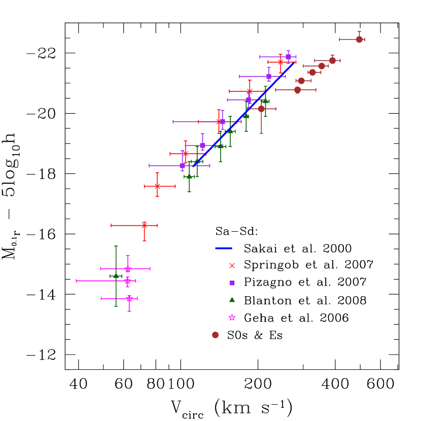
We use several datasets to construct the LV relation for observed galaxies. Springob et al. (2007) compiled a template -band Tully-Fisher sample of 807 spiral galaxies of types Sa-Sd in order to calibrate distances to galaxies in the local universe. Template galaxies were chosen to be members of nearby clusters in order to minimize distance errors. Their photometry contains distance uncertainties so the scatter should be taken cautiously and only as an upper limit to the intrinsic TF scatter. Circular velocities were obtained using HI line synthesis observations or optical H rotation curves when those were not available. The maximum circular velocity was obtained by using a model fit to the observed profiles. Since the authors correct for the effects of turbulence by subtracting linearly from the velocity widths, it was necessary to de-correct them by adding this term back in to obtain the true circular velocities.
The Pizagno et al. (2007) sample was selected from the Sloan Digital Sky Survey (SDSS) (York et al., 2000). It is one of the most complete and unbiased samples available of H rotation curves of disk galaxies and was studied in an attempt to accurately measure the intrinsic scatter in the TF relation. Luminosities were taken from SDSS -band photometry, yielding the best match with the luminosities assigned to our model galaxies. For this sample we used the asymptotic value of the rotation velocity they obtained using a functional fit to the rotation curves.
In order to test the predictions of the CDM model using abundance matching (CDM + HAM for short) with the largest dynamic range possible, we included in our comparison the latest Tully-Fisher dwarf galaxy sample studied by Geha et al. (2006). Their sample consists of about 110 late-type galaxies with luminosities measured in the -band and rotation velocities measured using HI emission.
The three samples above constitute our major observational dataset. We further cut them by selecting galaxies with high inclinations ( or axis ratio ) to minimize uncertainties due to projection effects. Additionally, we include only galaxies with better than accuracy in the measurement of the maximum circular velocity. These cuts leave a total of 972 galaxies in the major sample.
For comparison with the datasets mentioned above, we include other smaller samples found in the literature. The sample of Blanton et al. (2008) was also obtained from SDSS and is comprised of only isolated galaxies with high inclinations. The HI galaxy sample used by Sakai et al. (2000) was selected to have small scatter for use as a distance calibrator. It is important to note that while the fit shown here minimizes both the errors in rotation velocity and in luminosity, it may be artificially shallow due to selection effects.
Certain assumptions about galaxy colors had to be made in order to convert the different observational samples to the -band measurements we chose for our model. In order to convert the -band luminosities measured by Springob et al. (2007) to the -band, we cross-referenced their data with the sample of Pizagno et al. (2007) and used the median colors of the galaxies present in both catalogs. To convert from the -band magnitudes of Sakai et al. (2000) to the SDSS -band we used the transformation equations obtained by Lupton (2005) along with the typical color of disk galaxies in the SDSS sample studied by Blanton et al. (2003a). In addition, for redshift zero data sets, the k-correction given in Blanton et al. (2003b) was used to convert from to photometric bands.
Lastly, since the obscuring effect of dust extinction as a function of disk inclination is corrected for in Tully-Fisher samples but not in observed LF estimates, we had to de-correct the luminosities of the spiral galaxies in all of the TF samples. To do so, we estimated and added the median extinction in the -band as a function of rotation velocity using the method and sample employed by Pizagno et al. (2007). This correction is mag for the brightest disks, declining to mag for . These values are close to those found by Tully et al. (1998) for the extinction in a galaxy with average inclination as a function of HI velocity width. The correction is implemented only when comparing the observations with our model galaxies.
2.2 Early-type galaxies
We also include bulge-dominated early-type galaxies (ellipticals and lenticulars) in the LV relation, again measuring the circular velocity at our fiducial 10 kpc radius. The circular velocity in this case is used not as a measure of rotation but merely as a probe of the mass profile, further justifying the use of the term “LV relation” instead of TF relation. Using early-type galaxies allows us to probe closer to the mass regime where the abundance of DM halos drops exponentially (i.e., the knee of the velocity function), which is more sensitive to the cosmological model. It also allows for study of halo-galaxy relations without regard to the details of the evolution of the stellar populations within them.
Because of the challenges of both observing and modeling early-type galaxies, so far there exists no comprehensive set of mass measurements for them akin to the spiral galaxy samples. Instead, we compile a set of high-quality LV estimates for individual galaxies from the literature.
To provide the necessary LV data for nearby elliptical and lenticular galaxies, we searched the literature for high-quality mass measurements at radii. A variety of different mass tracers were used including hot X-ray gas, a cold gas ring, and kinematics of stars, globular clusters, and planetary nebulae. We required the mass models to incorporate spatially-resolved temperature profiles in the case of X-ray studies, and to take some account of orbital anisotropy effects in the case of dynamics. We also used only those cases where was constrained to better than 15%. We make no pretense that this is a systematic, unbiased, or especially accurate sample of early-type masses, noting simply that it is preferable to ignoring completely this class of galaxies which dominates the bright end of the luminosity function.
As an aside, we find in comparing to central velocity dispersions taken from HyperLeda (Paturel et al., 2003), that the scaling works very well on average, suggesting near-isothermal density profiles over a wide range of galaxy masses. It is far easier to measure observationally than , motivating the use of the former as a proxy for the true which is more robustly predicted by theory. The 15% scatter that we find in the – relation is relatively small, but it is beyond the scope of this paper to consider the potential systematics of using as a proxy. We will use for the LV analysis in this paper.
For the luminosities, we make use of the total -band apparent magnitudes from the RC3 (de Vaucouleurs et al., 1991), corrected for Galactic extinction. To correct to magnitudes, we use the filter conversions in Blanton & Roweis (2007) together with colors obtained from HyperLeda (Paturel et al., 2003). For the distances (required both for absolute magnitudes and for choosing the circular velocity measurement radii in kpc), we use as a first choice the estimates from surface brightness fluctuations (Jensen et al., 2003), and otherwise the recession velocity.
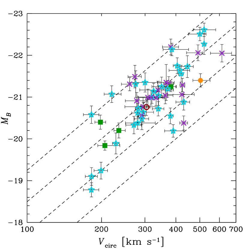
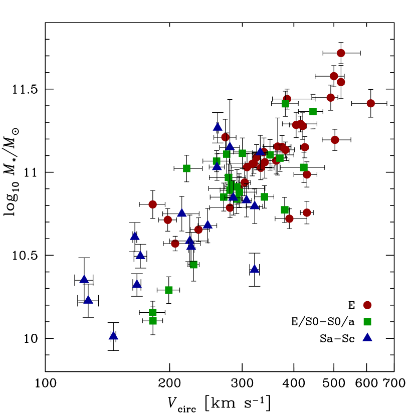
The local data for 55 individual early-type galaxies are presented in Figure 1 (left). Dashed lines show -band dynamical mass-to-light ratios of , 6, 12, and 24; for comparison, early-type galaxies with typical colors (–) are expected to have stellar – for a Chabrier IMF (e.g., Fig. 18 of Blanton & Roweis (2007)). A table including the sources of the data is provided in Appendix B. There is no obvious systematic difference between the results from different mass tracers. The galaxies appear to trace a fairly tight LV sequence, except around the luminosity (assuming ), where there are a few galaxies whose circular velocities appear to be fairly high or low. The low- galaxies include NGC 821 and NGC 4494, which were previously suggested as having a “dearth of dark matter” (Romanowsky et al., 2003), and as implying a dark matter “gap” with respect to X-ray bright ellipticals (Napolitano et al., 2009). The present compilation suggests that the galaxy population in the local universe may fill in this gap, although further work will be needed to understand the scatter.
The right panel of Figure 1 shows the relation between stellar mass and circular velocity at 10 kpc for the galaxies in the early-type sample along with a few spirals for comparison. Stellar masses were obtained using equation (8) as explained in Section 6.3. The ellipticals are virtually indistinguishable from the S0s in the regime where they overlap while the spirals seem to contain slightly more stellar mass at the same . We will discuss this issue in more detail in Section 6.3 .
2.3 Observational LV relation
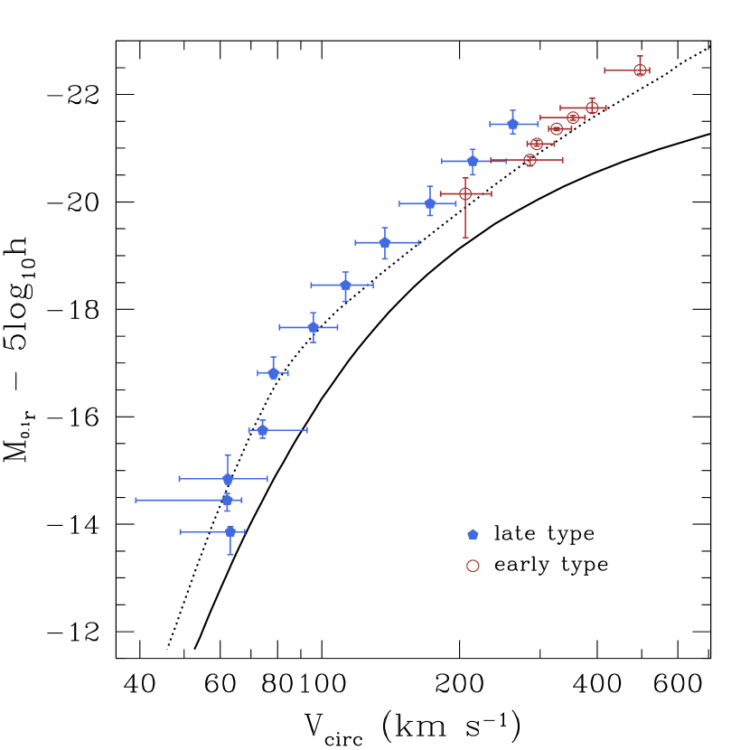
Figure 2 shows the combined LV relation for galaxies with very different morphologies: from Magellanic dwarfs with to giant ellipticals with . The LV relation is not a simple power-law. Dwarf galaxies show a tendency to have lower luminosities as compared with a simple power-law extrapolation from brighter magnitudes. There is a clear sign of bimodality at the bright end of the LV relation with early type galaxies having larger circular velocities as compared with spiral galaxies with the same -band luminosity (or, conversely, magnitude fainter at fixed ).
3 The Bolshoi simulation
The Bolshoi simulation was run using the following cosmological parameters: , , , , . These parameters are compatible with the WMAP seven-year data (WMAP7) (Jarosik et al., 2010) and with WMAP5 combined with Baryon Acoustic Oscillations and Type 1a Supernova data (Hinshaw et al., 2009; Komatsu et al., 2009; Dunkley et al., 2009). The Bolshoi parameters are in excellent agreement with the SDSS maxBCG+WMAP5 cosmological parameters (Rozo et al., 2009) and with cosmological parameters from WMAP5 plus recent X-ray cluster survey results (Klypin et al., 2010).
It is important to appreciate that Bolshoi differs essentially from another large, DM-only cosmological simulation: the Millennium simulation (Springel et al., 2005, MS-I). The Millennium simulation has been the basis for many studies of the distribution and statistical properties of dark matter halos and for semi-analytic models of the evolving galaxy population. This simulation and the more recent Millennium-II simulation (Boylan-Kolchin et al., 2009, MS-II) used the first-year (WMAP1) cosmological parameters, which are rather different from the most recent estimates. The main difference is that the Millennium simulations used a substantially larger amplitude of perturbations than Bolshoi. Formally, the value of used in the Millennium simulations is more than 3 away from the WMAP5+BAO+SN value and nearly 4 away from the WMAP7+BAO+H0 value. However, the difference is even larger on galaxy scales because the Millennium simulations also used a larger tilt of the power spectrum.
The Bolshoi simulation uses a computational box across and 8.6 billion particles, which gives a mass resolution (one particle mass) of . The force resolution (smallest cell size) is physical (proper) 1 kpc. For comparison, the Millennium-I simulation had a force resolution (Plummer softening length) 5 kpc and the Millennium-II simulation had 1 kpc. The Bolshoi simulation was run with the Adaptive-Refinement-Tree (ART) code, which is an Adaptive-Mesh-Refinement (AMR) type code. A detailed description of the code is given in Kravtsov et al. (1997); Kravtsov (1999). We refer the reader to Klypin et al. (2010) for more details specific to the use of the code for the simulation.
We use a parallel (MPI+OpenMP) version of the Bound-Density-Maxima (BDM) algorithm to identify halos in Bolshoi (Klypin & Holtzman, 1997). BDM does not distinguish between halos and subhalos111A subhalo is a halo which resides within the virial radius of a larger halo. – they are treated in the same way. The code locates maxima of density in the distribution of particles, removes unbound particles, and provides several statistics for halos including virial mass and radius, as well as density profiles222The Bolshoi halo catalogs are publicly available at http://www.multidark.org.. We use the virial mass definition that follows from the top-hat model in the expanding Universe with a cosmological constant. We define the virial radius of halos as the radius within which the mean density is the virial overdensity times the mean universal matter density at that redshift. Thus, the virial mass is given by
| (1) |
For our set of cosmological parameters, at the virial radius is defined as the radius of a sphere enclosing average overdensity equal to times the average matter density. The overdensity limit changes with redshift and asymptotically goes to 178 for high . Different definitions are also found in the literature. For example, the often used overdensity 200 relative to the critical density gives mass , which for Milky-Way-mass halos is about 1.2-1.3 times smaller than . The exact relation depends on halo concentration.
At each timestep there are about 10 million halos in Bolshoi (8.8 at , 12.3 at , 4.8 at ). The halo catalogs are complete for halos with km s-1 (). In order to track evolution of halos over time, we find and store the 50 most bound particles. Together with other parameters of the halo (coordinates, velocities, virial mass, and circular velocity) the information on most bound particles is used to identify the same halos at different moments of time. The procedure of halo tracking starts at and goes back in time. The final result is the history (track) of the major progenitor of a given halo.
4 DM halos: definitions and characteristics
We distinguish between two types of halos. A halo can be either distinct (not inside the virial radius of a larger halo), or a subhalo if it is inside of a larger halo. For both distinct halos and subhalos, the BDM halo finder provides the maximum circular velocity
| (2) |
Throughout this paper we will use term circular velocity to mean maximum circular velocity.
As the main characteristic of the DM halos we use their circular velocity . There are advantages to using as compared with the virial mass . The virial mass is a well defined quantity for distinct halos, but it is ambiguous for subhalos. It strongly depends on how a particular halo-finder code defines the truncation radius and removes unbound particles. It also depends on the distance to the center of the host halo because of the effects of tidal stripping. Instead, the circular velocity is less prone to those complications. The main motivation for using in this work is that it is more closely related to the properties of the central regions of halos and, thus, to galaxies hosted by those halos. For example, for a Milky-Way type halo the radius of the maximum circular velocity is about 40 kpc (and is nearly the same at 20 kpc), while the virial radius is about 200 kpc. In addition, the virial mass of a DM halo is not an easily observable quantity and this further limits its use for comparison of simulations with observations.
Tidal stripping can lead to significant mass loss in the periphery of subhalos. The net effect at redshift zero of the complex interactions that each halo undergoes is a decrease in the maximum circular velocity compared to its peak value over the entire history of the halo. The galaxy residing in the central region of the halo should not experience much stripping and should preserve most of its mass inside the optical radius (e.g., Nagai & Kravtsov, 2005; Conroy et al., 2006). Following this argument, the initial total mass distribution and rotation profile of the halo are frozen at the moment before the halo is accreted and starts to experience stripping. We refer to this circular velocity as . In practice we find the peak circular velocity of the halo over its entire history. Further details on the halo tracking procedure can be found in Klypin et al. (2010).
5 Connecting galaxies and DM halos
To investigate the statistics of galaxies and their relation to host DM halos as predicted by the CDM model using HAM, we obtained the properties of our model galaxies using the following procedure:
-
1.
Using the merger tree of each DM halo and subhalo, obtain the peak value of the circular velocity over the history of the halo (this is typically the circular velocity of the halo when it is first accreted). Perform abundance matching of the velocity function of the halos to the LF of galaxies to obtain the luminosity of each model galaxy.
-
2.
Perform abundance matching of the velocity function to the stellar mass function of galaxies to obtain the stellar mass of each model galaxy.
-
3.
Use the observed gas-to-stellar mass ratio as a function of stellar mass to assign cold gas masses to our model galaxies. The stellar mass added to the cold gas mass becomes the cold baryonic mass.
-
4.
Using the density profiles of the DM halos, obtain the circular velocity at () from the center of each halo. To do this, calculate the dark-matter-only contribution by multiplying the DM mass profile, obtained directly from the simulation, by the factor , where is the cosmological fraction of baryons333Recall that the Bolshoi simulation was run for a dissipationless cosmic density .. Then take the total cold baryon contribution from step 3 and assume it is enclosed within a radius of . Adding the two contributions gives the total mass required to calculate .
-
5.
Implement the correction to due to the adiabatic contraction of the DM halos due to the infall of the cold baryon component to the center.
We now explain each of the above 5 steps in detail.
Using the key assumption that halos with deeper potential wells become sites where more baryons can gather to form larger and more luminous galaxies, we ranked our halos and subhalos using their , and starting from the bright end of the -band LF, assigned luminosities to each according to their space density using the prescription found in Conroy et al. (2006). In other words, we found the unique one-to-one correspondence that would match the halo velocity function with the luminosity function of observed galaxies. Of course, this is a simplifying approximation. It does not discriminate between blue (star-forming) and red (quenched) galaxies, for example.
In this paper we use the Schechter fit to the -band galaxy LF measurement of Montero-Dorta & Prada (2009) obtained from the SDSS Data Release 6 (DR6) galaxy sample444To avoid aperture corrections when comparing to other data we use model magnitudes instead of Petrosian values.. The fit is characterized by the parameters: , , and . Since the median redshift of the SDSS DR6 sample is (Blanton et al., 2003a), all our subsequent results will be shown in -band magnitudes.
As an alternative, we also consider a LF with a steeper slope at low-luminosities. Blanton et al. (2005) obtained the SDSS LF including dwarfs as faint as and investigated surface brightness completeness at the faint end of the distribution. Their steeper value of the faint-end slope was obtained by weighting the abundance of each galaxy by its estimated surface brightness completeness. To quantify the effect of including low surface brightness galaxies in our model (those with Petrosian half-light -band surface brightness greater than 24.0 mag/arcsec2), we increased the abundance of bright galaxies in the Blanton et al. (2005) LF to match the Montero-Dorta & Prada (2009) LF at the bright end while keeping the steep faint-end slope () measured by Blanton et al. (2005). The modified LF produces 60% more galaxies at and over a factor of 2.5 more galaxies at . Using this LF to perform the abundance matching increases the luminosity of galaxies assigned to small DM halos, steepening the faint end of the LV relation.
It is important to note that we assume that each dark matter halo or subhalo must contain a galaxy with a detectable luminous component (for the SDSS -band this requires galaxies to be detectable in visible wavelengths) and this component must evolve in a way that guarantees its detectability at . Since the effective volume surveyed by SDSS DR6 at is comparable to the volume of the Bolshoi simulation, we expect the statistics of the halo population to be comparable to those of the observed galaxies all the way up to the large mass/luminosity tail of the distributions. Even though Bolshoi contains a factor of more objects than the sample of Montero-Dorta & Prada (2009), abundance matching is mostly insensitive to uncertainties in the high-luminosity tail of the LF.
5.1 The circular velocity of galaxies inside halos including cold baryons
The next step is to separate the DM and baryon components in each halo and allow the baryons to dissipatively sink to the centers of the DM halos. We assume for simplicity that there is a radius at which we could consider most of the cold baryons to be enclosed, with only dark matter present beyond that point.
This cold baryon component has been observed to comprise only a small fraction of the cosmic abundance of baryons; in other words, the cold baryon fraction in galaxies is much lower (Fukugita et al., 1998; Fukugita & Peebles, 2004) than (Komatsu et al., 2009). We resort to the observations and use the galaxy stellar mass function obtained from the SDSS DR7 by Li & White (2009), who employ estimates of stellar masses by Blanton & Roweis (2007) obtained using five-band SDSS photometry assuming the universal IMF of Chabrier (2003). These masses are consistent with those estimated using single-color and spectroscopic techniques (Li & White, 2009).
Using the same procedure described above for the luminosity function, we abundance-matched the halos in Bolshoi to the galaxies in the SDSS DR7 starting from the high stellar mass end until reaching our completeness limit at , obtaining stellar masses for each galaxy. Strictly speaking, this procedure results in a one-to-one relation between circular velocity and stellar mass-to-light ratio which should only be interpreted as the average of a population of galaxies with a given . The scatter (or bimodality) in the mass-to-light ratio as a function of circular velocity could be measured from observations and included in the assignment but would not change our results significantly.
Since dwarfs can have most of their cold baryons in the gas phase instead of in stars (Baldry et al., 2008), we calculated for each model galaxy the total cold gas mass using a parameterization of the observed atomic gas mass fraction as a function of stellar mass from Baldry et al. (2008) (their equation (9), shown as a dashed line in their Figure 11). This includes the total cold atomic gas found in the disk only. The gas-to-stellar mass ratio depends on stellar mass and it is the largest for dwarfs. For example, for galaxies with . It declines to for galaxies with . It should be even smaller for ellipticals and S0s. It should be noted that, when it comes to dynamical corrections to , the gas plays a minor role. It only becomes important when we consider the baryonic Tully-Fisher relation.
Lastly, we add the stellar and cold gas masses for each model galaxy and obtain the correction to the circular velocity of the pure DM halo at a radius enclosing the cold baryonic mass. We set this value to for all the halos in our sample. In the case of dwarf galaxies this should be a good approximation to the maximum circular velocity since their rotation curves rise much more slowly and in some cases they peak beyond the optical radius (Courteau, 1997). Our assumption allows us to include the peak of the rotation curve for most of these galaxies. In the case that the peak is located well within the correction would be almost negligible since we would be still measuring rotation in the flat regime. Additionally, truncating the cold baryons at a radius of allows us to directly calculate the correction to the circular velocity at that radius without having to resort to more complicated assumptions about the distribution of baryonic matter in galaxies, i.e., exponential lengths and Sérsic indices of disks and bulges as well as extended gas and stellar halos.
To obtain the circular velocity measured at () for the Bolshoi DM halos, we need to use dark matter profiles and find the dark matter mass inside a 10 kpc radius. To do this, we could use the individual profile of each halo. However, once we select halos with a given maximum circular velocity, individual halo-to-halo variations are small at 10 kpc (the situation is different if we select halos using virial mass, which results in large deviations in concentration producing large variations in ). This is why instead of individual profiles we construct average profiles for halos within a narrow range of maximum circular velocity.
We first bin and average the circular velocity profiles of the distinct halos found by the BDM code. These profiles are calculated for each halo (including unbound particles) in logarithmic radial bins in units of . Using distinct halos is convenient because it gives us density profiles that are less affected by interactions than those of subhalos. For the inner profiles of subhalos the effect is relatively small because the stripping happens preferentially at the outer radii. Using the averaged binned circular velocity profiles we obtain the velocity at . Within about of the virial radius, discreteness effects render the profiles unreliable and we use instead extrapolation with the shape of a simple power-law in radius. For halos with the full extent of the profiles suffer from measurement noise which we avoid by extrapolating from the profile of halos with . Figure 3 shows the obtained median relation between the maximum circular velocity and for the Bolshoi DM halos without inclusion of the cold baryons.
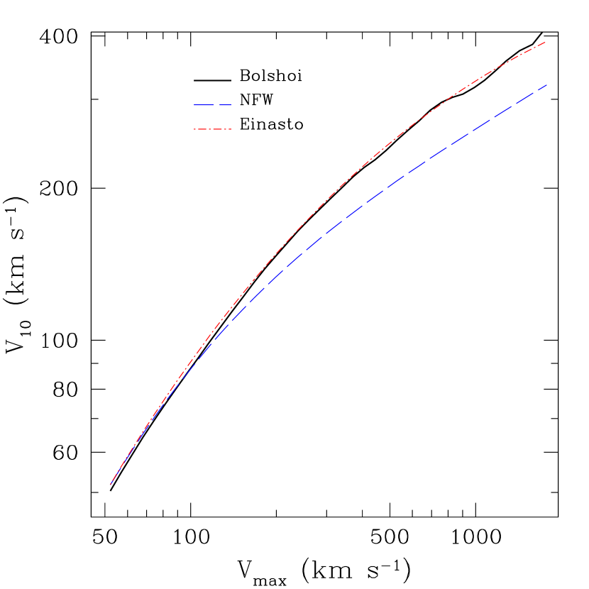
The estimates of the relations obtained when a parametric form of the density profile is used are also shown for the case of the NFW (Navarro et al., 1997)
| (3) |
and the Einasto (Einasto, 1965; Graham et al., 2006) universal profiles
| (4) |
where is the radius at which the logarithmic slope of the density profile is . Following Graham et al. (2006), we use . The concentration parameter defined for both models as is given by the relations obtained in Paper I for distinct halos (Klypin et al. 2010; see also Prada et al. 2011) :
| (5) |
and
| (6) |
Note that in Figure 3 we use total dynamical masses and do not account for the condensation of baryons. For the rotation (or density) profiles of the Bolshoi simulation are extremely well approximated by the Einasto parameterization, whereas NFW underestimates by almost at . Following the conclusions of Navarro et al. (2004) and Graham et al. (2006), we assume the Einasto profile when extrapolating the inner parts of the largest () halos.
5.2 Adiabatic contraction of DM halos
Dissipation allows the baryons to condense into galaxies in the central regions of DM halos dragging the surrounding dark matter into a new more concentrated equilibrium configuration. If the density of the DM halo increases considerably within the extent of the disk, the peak circular velocity could be much larger than our previous estimates. There are different approximations for the adiabatic compression of the dark matter. Blumenthal et al. (1986) provide a simple analytical expression, which is known to overpredict the effect. The approximation proposed by Gnedin et al. (2004) predicts significantly smaller increase in the density of the dark matter. More recent simulations indicate even smaller compression (Tissera et al., 2009; Duffy et al., 2010). However, at a 10 kpc radius the dark matter contributes a relatively large fraction of mass even for large galaxies. As a result, the difference between the strong compression model of Blumenthal et al. (1986) and no-compression is only % in velocity.
We use the standard adiabatic contraction (AC) model of Blumenthal et al. (1986) to bracket the possible effect. We thus assume that following the condensation of the baryons, the dark matter particles adjust the radius of their orbits while conserving angular momentum in the process. We solve the equation
| (7) |
where , is the total baryonic mass assigned to each halo and is the universal fraction of baryons. We solve equation (7) for and then add the dark matter mass to the mass of cold baryons to find the circular velocity. Note that this implies that only cold baryons (i.e., stars and cold gas) are left in the central regions of the galaxy, while the remaining hot baryons are at larger radii. As expected, only the halos that are dominated by baryons at their centers suffer a significant increase in their measured circular velocities due to the increase in concentration of dark matter as result of adiabatic contraction.
6 Results
6.1 The Luminosity-Velocity relation
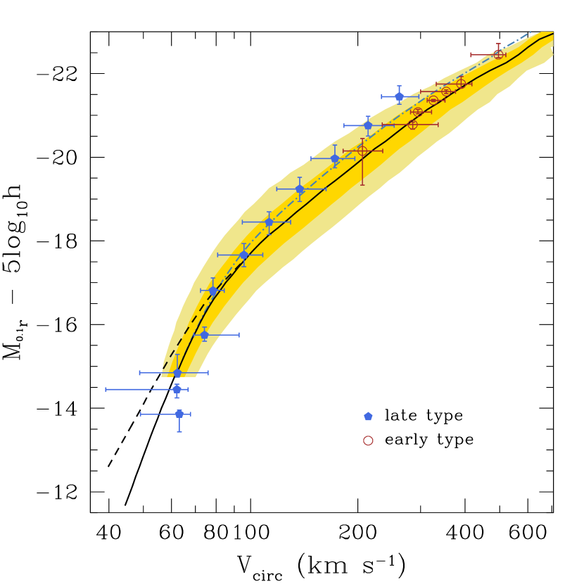
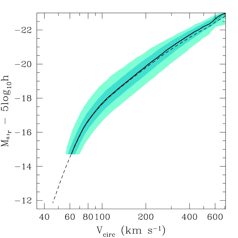
Figure 4 shows the predicted LV relation for galaxies in the CDM model obtained using halo abundance matching. We binned together the major observational samples described in Section 2 and include them for comparison. The internal extinction de-correction for late-type galaxies described in Section 2.1 was implemented for a fair comparison with the models. The full curve in this plot shows results obtained using the Montero-Dorta & Prada (2009) LF of galaxies in the SDSS DR6 sample and uses the adiabatic contraction model of Blumenthal et al. (1986). The 1- and 2- width of the distribution of model galaxies in bins of luminosity is represented by the shaded regions (details about the model used to add scatter can be found in Section 6.2.4). Predictions without adiabatic contraction (with the cold baryon contribution added in quadrature) are shown as the dot-dashed curve. The dashed curve shows the effect of a steeper slope at the faint end of the LF that accounts for potential surface brightness incompleteness. (For details see Section 5). Although dwarf galaxies with seem to agree better with a model using the Montero-Dorta & Prada (2009) luminosity function, the scatter of the observed dwarf LV relation is so large that both LFs used in conjunction with the abundance of DM halos produce results that are consistent with the available data.
One may note that the AC model misses late-type points with and the no-AC model practically fits most of the late-type measurements. This should not be interpreted as either an advantage for the no-AC model or a disadvantage for the AC model. Our predictions apply to the average population across all types of galaxies. Because of the dichotomy of the LV diagram, a model that goes through either early-type galaxies or through late-type galaxies is an incorrect model. The correct answer should be a model which tends to be close to spirals at low luminosities (where spirals dominate the statistics) and gradually slides towards the ellipticals at the high-luminosity tail where they dominate. It seems that the AC model does exactly that, but it may overpredict the circular velocities at the very bright tail of the LV relation.555Schulz et al. (2010), Napolitano et al. (2010) and Tortora et al. (2010) find observational evidence for AC in elliptical galaxies.
As demonstrated in Section 6.2.4, our stochastic HAM model accounts for galaxies that reside in halos with both smaller and larger than the average. For example, since the most massive spiral galaxies comprise a very small percentage of the galaxy population with (less than 10%), in our model they are assigned to the low- wing of the distribution shown in Figure 4. Hence, even though the model makes predictions for the average galaxy population, it also accounts for the morphological bimodality observed in the LV relation.
One also should not overestimate the quality of the observations. The fact that in Figure 4 the brightest spirals with are more than 2- away from the mean of the models is not a problem because of the size of the uncertainties in the observational data. For instance, there is a systematic % velocity offset between the measurements of Pizagno et al. (2007) and Springob et al. (2007), which seems to point to the current uncertainties in the LV relation.
Considering the current level of the uncertainties, our model galaxies show remarkable agreement with observations spanning an order of magnitude in circular velocity (or, equivalently, three orders of magnitude in halo mass) and more than three orders of magnitude in luminosity. For galaxies above , our model produces results that agree extremely well with the observed luminosities of early-types (Es and S0s). Given how simple the prescription is, it is perhaps surprising how closely we can reproduce the properties of observed galaxies. For galaxies with , DM halos without any corrections already occupy the region expected for galaxies. The dynamical corrections improve the fits, but it is important to emphasize that the abundance matching method yields the correct normalization of the LV relation regardless of the details of the corrections we implement. Another feature of the relation, its steepening below , is caused by the the shallow faint-end slope of the luminosity function. Although our model galaxies in this regime are slightly underluminous as compared with a simple power-law extrapolation from brighter galaxies, observed dwarfs seem to predict a deviation from a power-law TF in the same general direction.
In the way it was constructed, our model galaxy sample does not include uncertainties in either the halo velocity function or in the galaxy luminosity function. This produces an LV relation with no scatter. Section 6.2.4 examines the effects of including scatter in the halo matching procedure.
We now discuss in greater detail the results of the individual steps explained in Section 5.
6.2 The Luminosity-Velocity relation: detailed analysis of model components
6.2.1 Measuring circular velocity at 10 kpc
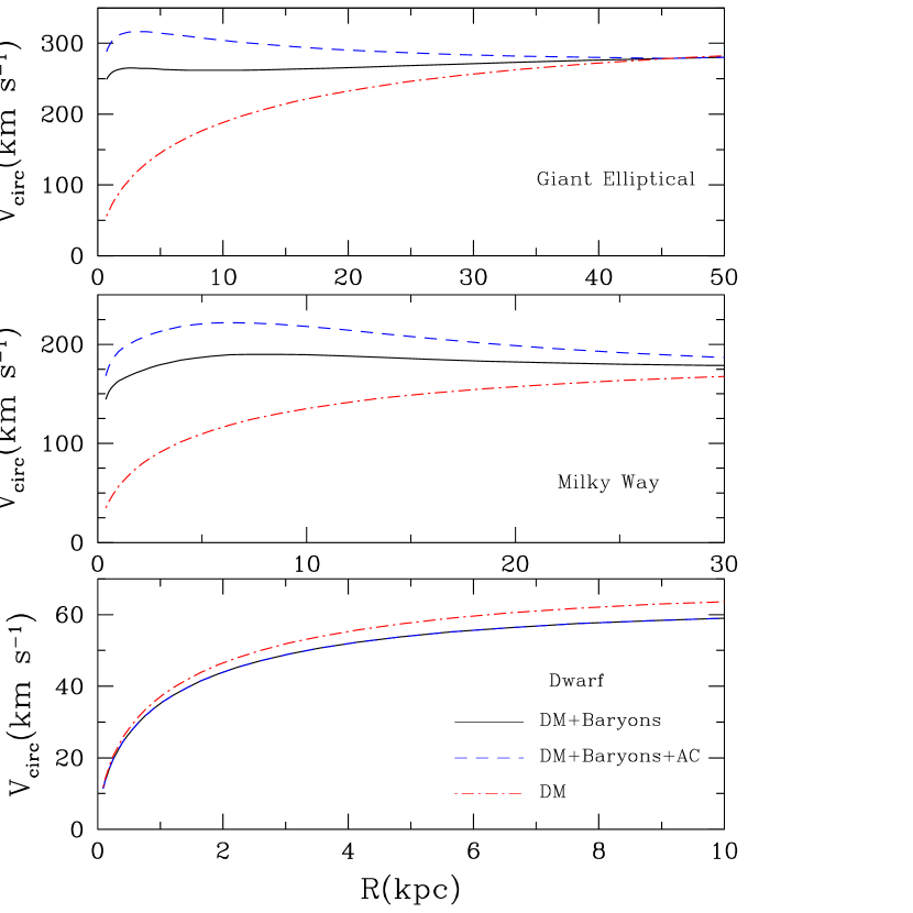
Observations do not always provide measurements of the circular velocity at 10 kpc. This is especially true for dwarf galaxies where the last measured point of the rotation curve can be at 3-5 kpc. What are the errors associated with using measurements at different radii? Figure 5 presents three typical examples of the circular velocities expected for galaxies with vastly different masses.
The top panel shows a model of a giant elliptical galaxy with of stellar mass distributed according to a law with a half-light radius of kpc. The stellar component is embedded in a dark matter halo with virial mass and median concentration . The maximum circular velocity (310 km s-1) of the halo is reached at 160 kpc. The middle panel shows a Milky Way-size model with maximum circular velocity 190 km s-1, virial mass , and median concentration for its mass. The cold baryonic component consists of a Hernquist bulge (, half-mass radius kpc) and an exponential disk (, scale radius kpc). The bottom panel shows a dwarf galaxy model with , , km s-1. Its cold baryons have two exponential disks: one for stars and and one for cold gas with a mass ratio of 1:4 and radii kpc and kpc. The total mass in cold baryons is . When we include baryons, we assume that most of them were blown out from the models and the only baryons left are in the form of stars and cold gas. As in Bolshoi, the “DM” circular velocities in Figure 5 include a cosmological amount of baryons that traces the distribution of the dark matter. This contribution is removed from the mass profiles before adding the cold baryons. In all three cases we use the Einasto dark matter profiles (equation (4)) with . For the models labeled “DM+Baryons” at each radius we simply add the mass of cold baryons and the mass of dark matter. The models termed “DM+Baryons+AC” include adiabatic compression of dark matter according to the prescription of Blumenthal et al. (1986).
After adding the cold baryons the circular velocity profiles become rather flat in the inner kpc regions of the galaxies implying that measurements of circular velocities anywhere in this region are accurate enough to provide the value of the circular velocity at 10 kpc.
There are some caveats in choosing 10 kpc as a fiducial radius for either extremely massive spirals or giant ellipticals. Considering the correlation between central surface brightness and disk scale-length found by Courteau et al. (2007), the most luminous disks appear to have scale-lengths as large as , whereas according to Courteau (1997) their rotation curves peak at about 1 scale-length. Hence, we may be underestimating the maximum observed rotation velocity of these galaxies in our sample. We may also overestimate circular velocities when we assume that most of the cold baryon mass is inside 10 kpc radius. In principle, some corrections can be applied to compensate this effect. However, our estimates show that at most this is a % effect for spirals and somewhat smaller for ellipticals because they are more compact for the same luminosity. Considering existing uncertainties and complexities of implementing the correction, we decided not to use them.
6.2.2 Dark matter profiles
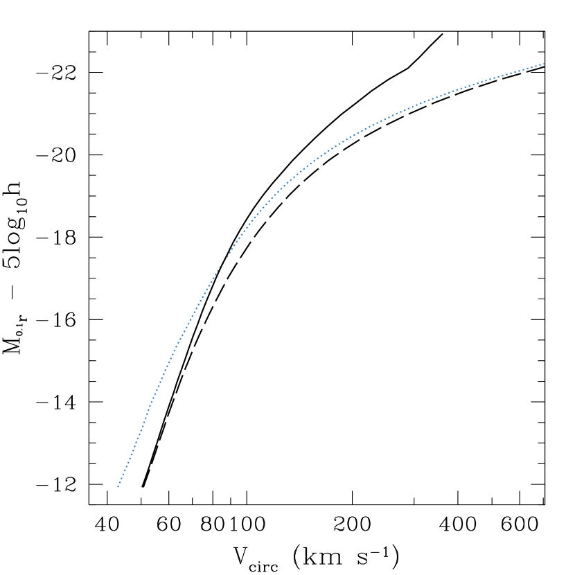
To illustrate the effect of tidal stripping, Figure 6 shows the results (dashed curve) obtained when the luminosity assignment is performed using the peak historical value of each halo’s circular velocity () as compared with the circular velocity at (dotted curve). The reason why the dashed curve is rightwards of the dotted one is that for subhalos the circular velocity estimated at is smaller than its value at accretion . If we compare luminosities at the same circular velocity, the differences can be substantial: almost one magnitude for galaxies with km s-1due to the steep slope of the LV relation for dwarfs. In terms of velocities, the differences are much smaller. Neglecting the effects of stripping in the assignment scheme affects mostly dwarf galaxies, overestimating their circular velocities by a maximum of . For larger galaxies the effect decreases to less than . This is due to the fact that stripping only affects subhalos and they comprise only a minority (about ) of the total halo population. In addition, only the small number of subhalos which orbit close to their host halo’s center get significantly stripped and experience a substantial decline in their circular velocity.
Comparison of LV relations constructed using one with the maximum the circular velocity (the dashed curve in Figure 6) and another with velocities estimated at 10 kpc (the full curve) indicates that this affects the largest halos the most. For example, the velocity is almost a factor of two smaller than for the group-size halos presented in the plot. Taking the circular velocity at 10 kpc also makes the LV relation much less curved as compared with the maximum velocity. Below the maximum circular velocity of the DM halo happens near or within 10 kpc, which explains why the curve does not shift in this regime.
6.2.3 The effects of cold baryons and adiabatic compression
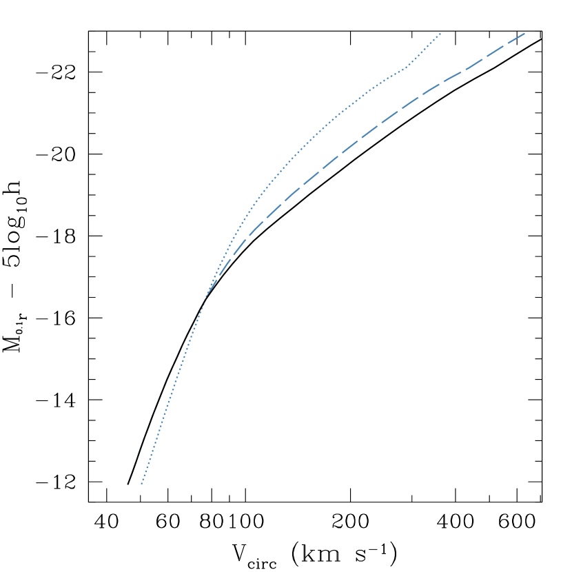
Figure 7 shows how cold baryons change the circular velocity at a 10 kpc radius. Here we use two extreme approximations that bracket the effect. The first approximation assumes that there is no change in the distribution of the dark matter. All simulations so far indicate that there is some compression. Hence, the no compression approximation definitely underpredicts the circular velocity . The second approximation uses the adiabatic compression model of Blumenthal et al. (1986) which produces the largest increase in the density of the dark matter. (The full and dashed curves were already shown in Figure 4). There are some differences between the LV relations predicted by those approximations. However, the largest effect is just adding the cold baryons in quadrature to the circular velocity of the dark matter. Adiabatic compression increases the circular velocity even further, but the effect is relatively minor because the fraction of cold baryons gets progressively smaller for larger galaxies. The amount of cold baryons used for the models is crucial for this test. As we discuss in Section 6.3, the abundance matching predicts relatively small cold baryon masses for dwarfs and giants, and this is why the adiabatic compression in Figures 5 and 7 is 10-20% at the most. Again, dwarfs below are insensitive to the cold baryon presence. Here the full curve (DM+baryons) is slightly below the of the dark matter curve because the latter includes a cosmological fraction of baryons which trace the DM, most of which are assumed to be blown out from galaxies (see Section 5).
Figure 8 shows the LV relation that we would obtain by assuming instead that half of all baryons within the virial radius or equivalently 8% of the virial mass are retained and are used to build the central galaxy (while luminosity is not affected). Both the shape and the normalization of the LV relation are incorrect, with the circular velocities systematically larger than observations by up to . Clearly, it is difficult to obtain the observed LV relation assuming a constant cold baryon fraction in the framework of the CDM cosmology.
6.2.4 The effects of including scatter in luminosity at fixed halo circular velocity
So far, the abundance matching procedure we have used assumed a monotonic one-to-one relation between halo circular velocity and galaxy luminosity or stellar mass. This assumption produces average relations that can be compared with the medians of the observations. As shown by previous studies, a more detailed treatment of the scatter between halo and galaxy properties may yield average relations of the brightest galaxies that deviate significantly from the case with no scatter. For instance, Tasitsiomi et al. (2004) showed that iteratively introducing log-normal scatter of width mags in the assignment of luminosities to DM halos produces an average TF relation with massive galaxies that are brighter by about one magnitude compared to the monotonic assignment. By treating the scatter analytically, Behroozi et al. (2010) found that performing halo abundance matching using their preferred value of dex of log-normal scatter reduces the average stellar mass assigned to massive halos with total masses by up to (when binning using virial mass) but does not affect less massive galaxies below the knee of the stellar mass function.
Appendix A gives a detailed description of the method we employ to introduce scatter in our model. In short, we obtain luminosities for each of the galaxies in our sample by stochastically scattering the values obtained in the monotonic assignment while forcing the preservation of the observed luminosity function. When scattering the values of luminosity we do not constrain the shape of the probability distribution (e.g., log-normal) or require its width to be constant for all circular velocities. This is well justified since the shape of the intrinsic scatter is more difficult to constrain observationally (e.g., due to observational systematics).
One parameter that our model does not currently predict is the width of the probability distribution of luminosity at a fixed halo circular velocity. This scatter originates from three main sources. The first is the observational error in the determination of the true luminosities of galaxies. Since we use the LF from the SDSS spectroscopic sample, these are the sum of the errors in photometry plus the errors in the distances obtained from spectroscopy. At the mean redshift of the sample these combined errors are expected to be typically much less than mags. The second source of scatter is the one present in the intrinsic relation between halo circular velocity and galaxy luminosity due to variation in the physical processes of galaxy formation. Verheijen (2001) studied the nature of the intrinsic scatter in the Tully-Fisher relation from HI observations and obtained a value of in the R-band. This value is consistent with the distribution in the observational samples used in this work. Lastly, since we assign luminosities that are uncorrected for the inclination of disk galaxies, we also need to include the scatter that results from the distribution of dust extinction corrections observed in SDSS. Maller et al. (2009) find a fit to this distribution as a weak function of -band luminosity and disk scale length. We adopt the value they use for a galaxy with . We neglect the errors due to photometry and distances and add the remaining two contributions in quadrature to obtain , which we use to introduce scatter to the model galaxies below the knee of the LF. Above this luminosity, where early-types dominate, we assume that the lack of significant internal extinction slightly reduces the scatter to .
Figure 9 shows the luminosity-binned distribution of model galaxies in the LV relation obtained from the stochastic HAM scheme and compares it to the monotonic assignment discussed in Section 6.1. Since we are left with a choice regarding which quantity to average over, we choose to bin in -band magnitude to be consistent with the binning of the observations. The mean relation is almost identical to the case with no scatter for galaxies below , while it becomes brighter by up to magnitudes for more massive galaxies. Galaxies below show a distribution of luminosities that is close to gaussian as far as 2- away from the mean but has a slightly longer bright tail. Galaxies brighter than show a trend of narrowing of the distribution as well as a skewness that reduces the number of upscattered galaxies with increasing luminosity.
To check the consistency of our approach we also calculated the average LV relation of our model galaxies obtained using the deconvolution method described in Behroozi et al. (2010) and log-normal scatter. This procedure yields a deviation of the mean relation for towards higher luminosities that depends on the assumed width of the scatter. Figure 17 in Appendix A shows this effect for constant (left panel) and decreasing from 0.5 to 0.3 past (right panel). Even with a variable width that mimics our approach, the luminosity-binned spread obtained with the method of Behroozi et al. (2010) is unrealistically large at the bright end.
The differences between the results of the two methods actually reside in the assumptions about the shape of the spread. Since our stochastic assignment scheme does not constrain the scatter distribution to be log-normal and centered on the monotonic relation, the resulting skewness beyond allows it to preserve the median LV relation of the scatterless sample. In addition, without a skewed distribution it is extremely difficult to obtain a narrower distribution of galaxies at the bright end of the LV relation.
From this analysis we conclude that the introduction of scatter in luminosity at a given halo circular velocity yields a median relation at the bright end that is sensitive to the shape and width of the probability distribution function used. The median LV relation is thus robust to uncertainties in the nature of the scatter below the shoulder of the LF, allowing for a direct comparison with observations. We prefer our scatter method for two reasons. First, it exactly preserves the luminosity function while the deconvolution method only does so approximately. Second, it naturally produces an observed luminosity-binned distribution that becomes narrower for the brightest galaxies, in agreement with that expected from observations.
6.3 Baryon fraction and the baryonic Tully-Fisher relation
For the LV relation the cold baryons played an ancillary role: they provided a correction to the circular velocity at 10 kpc. The correction is small for galaxies below . For large galaxies the cold baryon contribution increases and typically is about half of the mass within . Regardless of their role in the LV relation, baryons are one of the prime subjects for the theory of galaxy formation. Unfortunately, accurate measurements of baryonic masses are also prone to some uncertainties. Dynamical measurements of the baryonic component are difficult because of dark matter-baryon degeneracies (e.g., Dehnen & Binney, 1998). In other words, the baryon mass depends on what is assumed about the dark matter. Population synthesis provides an independent estimate of the stellar mass, but it has its share of complexities including the uncertainty in the initial mass function. In addition to the stellar mass, most galaxies have an important (if not dominant) fraction of their cold baryons in the form of neutral hydrogen gas. For consistency, in this paper we make use of stellar population synthesis estimates of stellar masses whenever possible.
The baryonic Tully-Fisher relation (BTF) is one way of displaying the amount of cold baryons in galaxies. The BTF relation has been investigated over the years (McGaugh et al., 2000; Bell & de Jong, 2001; Verheijen, 2001; McGaugh, 2005; Stark et al., 2009; McGaugh et al., 2010). Here we use the recent observational samples of Stark et al. (2009) and Leroy et al. (2008), along with Verheijen (2001) and the Geha et al. (2006) sample used for the LV relation. Stark et al. (2009) include gas-dominated spiral galaxies, which makes the results much less sensitive to the uncertainties in the IMF. For consistency, we calculate stellar masses for the Stark et al. (2009) and Geha et al. (2006) samples using a simple linear fit to the distribution of -band mass-to-light ratios vs. color shown in Figure 18 of Blanton & Roweis (2007):
| (8) |
Unlike the Bell et al. (2003) models, this relation fits well the measured mass-to-light ratios of both blue and red galaxies in the SDSS. These estimates are fully compatible with the stellar masses used in the stellar mass function of Li & White (2009) as part of our model. Leroy et al. (2008) present results based on the HI Nearby Galaxy Survey (THINGS): Walter et al. (2008). The measurement of luminosities in the infrared using Spitzer results in reliable estimates of the stellar masses that are consistent with the Blanton & Roweis (2007) results. In this case we adjust their stellar masses from the Kroupa to the Chabrier (2003) IMF used by Blanton & Roweis (2007) by subtracting 0.05 dex. Selecting only galaxies with high inclinations ( or ) and better than 15% accuracy in the circular velocity data leaves a total of 161 galaxies. We also include the results of mass modeling of the Milky Way and M31 (Klypin et al., 2002; Widrow & Dubinski, 2005).
We also employ equation (8) to obtain stellar masses for the early-type galaxies. This ensures a fair comparison between the baryonic masses of early- and late-type galaxies.

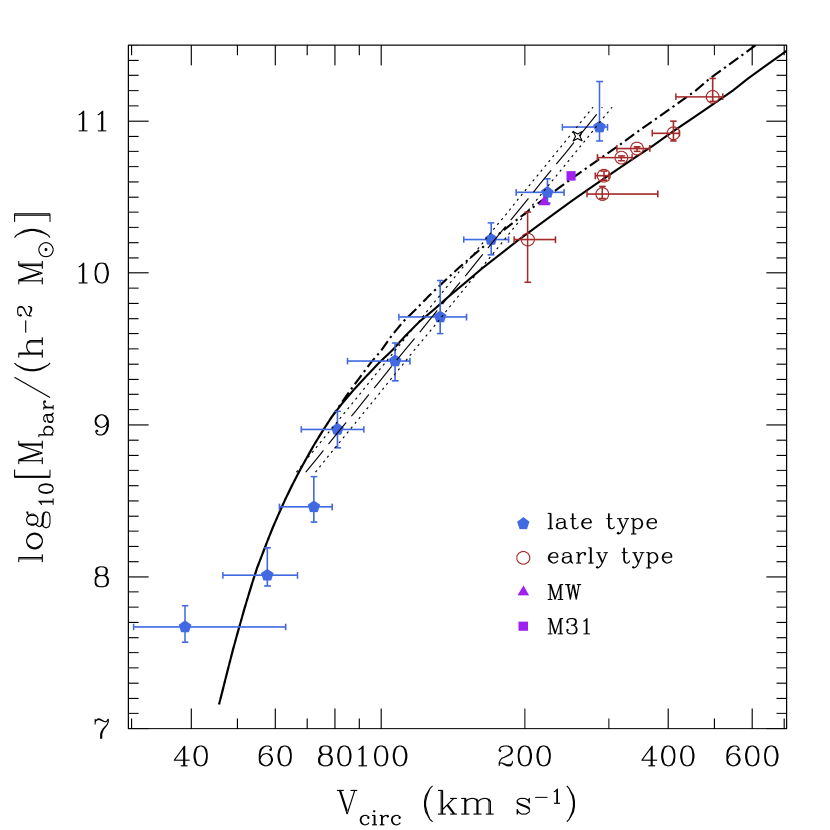
Figure 10 shows the cold baryon fraction relative to the universal value as a function of stellar mass in our model. The cold baryon fraction peaks at for the stellar masses typical of Milky Way-type galaxies and sharply falls on both sides of the mass spectrum. Our results are broadly consistent with Guo et al. (2010). We note that even the peak of is almost a factor of two smaller than what a few years ago was considered a fiducial value (Mo et al., 1998).
The baryonic Tully-Fisher relation is shown in Figure 11. Theoretical estimates from abundance matching provide a good fit to observational results for galaxies ranging from dwarfs with to giants with . In a remarkable agreement with the LV relation result, the model with adiabatic contraction seems to also provide a better fit to the BTF compared to the model with no contraction. There is a hint that observations show more baryonic mass for dwarfs below as compared to an extrapolation of the model. It is not clear whether this is a real problem because of the uncertainties involved in the observations. FIrst, the small sample size could produce biased results. Second, there is an uncertainty at the faint end of the luminosity function. The results of abundance matching are sensitive to the number density of galaxies with absolute magnitudes , which is poorly constrained.
As in the case of the LV relation, the model BTF relation agrees very well with the average population of galaxies in each morphological regime. Below it follows late-type disks while it accurately describes massive early types above this threshold. The observations show no preference for a model with no halo contraction vs. one with maximum contraction. Both cases fit well within the systematic and statistical uncertainties in the observations.
Although S0 and elliptical galaxies seem to contain slightly less mass in cold baryons than massive spirals, there is also a hint that the bimodality observed in the observed LV relation in Figures 2 and 4 between early- and late-type galaxies is not merely the result of a variation in the mass-to-light ratio. Other authors have come to the same conclusions (e.g., Williams et al., 2010; Dutton et al., 2010a, b). This would imply that early types are not just the result of passive fading of late-type disks but are fundamentally different. It also requires that they inhabit deeper potential wells which may be the result of different formation or environmental processes. These results have deep implications for galaxy formation but in order to draw conclusions we would need consistent stellar and gas mass estimates for a larger sample of galaxies, which are not currently available.
6.4 Galaxy Circular Velocity Function
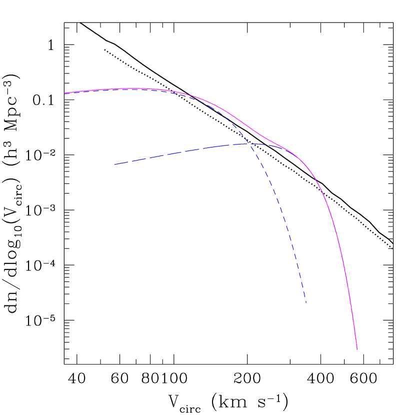
Projecting the distribution of galaxies in the LV plane onto the luminosity axis produces the luminosity function, while projecting onto the circular velocity axis yields the circular velocity function (VF) of galaxies: the number-density of galaxies with given circular velocity. From a theoretical cosmology point of view, the VF is an ideal characterization because it does not include uncertain predictions for the luminosity and requires relatively modest corrections for the baryonic masses. Unfortunately, it is more difficult to obtain it from observations and so far, there have been only a few attempts to do so (Gonzalez et al., 2000; Kochanek & White, 2001; Zavala et al., 2009; Chae, 2010; Zwaan et al., 2010).
For the theory the starting point is the velocity function of dark matter halos (e.g., Klypin et al., 2010). For halos with it is well approximated by a power-law , where . This only applies to velocities taken at the maximum of the circular velocity curves of DM halos. For galaxies, the results must be adjusted to and corrected for the dynamical effects of cold baryons.
The most recent measurement of the VF of nearby late-type galaxies was obtained by Zwaan et al. (2010). Their result is based on the blind HI sample of the HIPASS survey, which is complete down to at a distance of (Zwaan et al., 2010). Since gas-rich galaxies are thought to dominate at the low mass end, their sample should provide an accurate measurement of the abundance of dwarfs if these galaxies contain enough neutral gas to be detected. To obtain a galaxy velocity function for all morphological types we also include the determination of the early-type VF done by Chae (2010), using the conversion between velocity dispersion and circular velocity found in Zwaan et al. (2010). Even though their VF was obtained indirectly using the observed relation between luminosity and stellar velocity dispersion, it agrees with previous direct measurements.
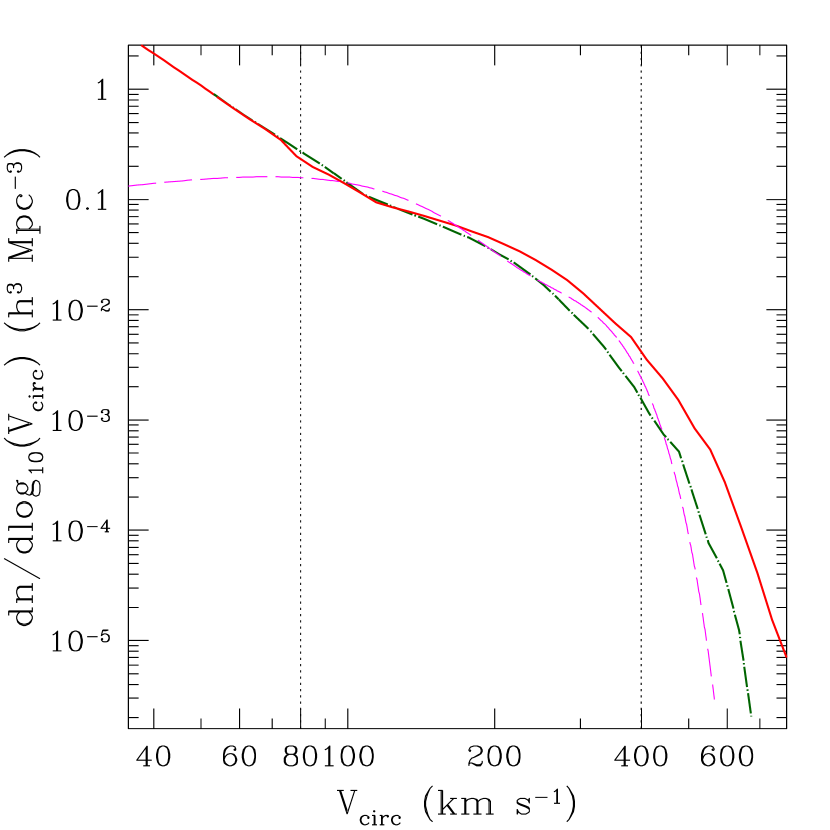
Figure 12 shows the results, as well as the modified Schechter fit to the VF of late-type galaxies (Zwaan et al., 2010) and the fit for early types found in Chae (2010). At intermediate to large masses (), where the completeness of the surveys is hard to question, the VF of our model sample reproduces the observed abundances reasonably well. The abundance of MW-type galaxies is predicted to within when adiabatic contraction is taken into account, and within a few percent when no contraction takes place. From our earlier analysis of the LV relation in Section 6 we are led to believe that halo contraction is needed to obtain the correct position of elliptical and S0 galaxies in the plot. A more detailed treatment of AC might be necessary in order to better match the abundance of galaxies larger than the Milky Way. Our model galaxy VF overestimates the abundance of the most massive and rarest galaxies with regardless of whether or not we implement the correction for contraction of the halos. Most of these extremely bright galaxies inhabit the centers of clusters, where it is very likely that the simplistic observational estimate of is breaking down. At small velocities () the theory significantly overpredicts the number of dwarfs. This “missing dwarfs” problem remains unresolved in CDM (Tikhonov & Klypin, 2009; Zavala et al., 2009; Zwaan et al., 2010). It should be noted that the variance of the velocity function of the model galaxies below in regions of radius can be as large as 1 order of magnitude. This shows that environmental bias may be an important factor in explaining the underabundance of dwarfs in our model compared to HIPASS.
To illustrate the effect that each of the steps in our procedure has on the VF, we show in Figure 13 the VF of DM halos only. It also shows that when the stripping due to the merger history of each halo is considered, the halo VF does a slightly better job at matching the abundance of galaxies.
As we previously noted, the corrections due to the presence of the cold baryonic component affect dwarfs () very little, resulting in a negligible shift in their abundance compared to that of their host DM halos at the low-mass end of the VF in Figure 12. One interpretation of this is that the dwarf overabundance problem cannot be resolved if both the LV relation and the VF of dwarf galaxies are to be reproduced simultaneously. In other words, these galaxies must undergo a process that limits their abundance without changing their dynamical mass. The first possible origin for the large discrepancy between our model galaxies and the HIPASS VF could be observational bias. HIPASS is a blind HI survey and does not detect gas-poor galaxies. Only if gas-poor dwarf spheroidals dominate the galaxy population below would it be possible to reconcile our results with the survey. This is highly unlikely since this type of galaxies are only a small fraction of the total dwarf population. On the other hand, if the HIPASS HI mass detection limit ( at ) is relatively high at the distances where most of their sample is found, incompleteness effects might explain the discrepancy.
Assuming that the surveys are complete, a possible solution to the problem is a mapping of all the dwarf galaxies below to DM halos in the range . This in turn implies that the measured rotation curves of a large fraction of dwarfs must severely underestimate the true maximum circular velocities of these galaxies. The only possible explanation for this bias would be that the optical and HI disk is truncated well inside the radius where the rotation curve flattens out. Another solution to the missing dwarf problem requires most of these galaxies to have a low enough surface brightness in HI to be undetectable in current surveys. This would imply the existence of a large number of small halos containing little or no neutral gas.
6.5 Galaxy two-point correlation function
The most important success of the halo abundance matching technique is considered to be reproducing the observed galaxy clustering measured in the form of the galaxy correlation function in its various forms, both in the local universe and at high redshift (Tasitsiomi et al., 2004; Conroy et al., 2006; Guo et al., 2010; Wetzel & White, 2010). Most of these works claimed to match the observed clustering although they relied on simulations with either very low resolution or outdated cosmological parameters. The high resolution and large volume of the Bolshoi simulation allow us to calculate the galaxy two-point correlation function at a range of scales comparable to the latest results from the final data release of the SDSS (Zehavi et al., 2010). In addition, its up-to-date set of cosmological parameters allows for a direct comparison between observations and the predictions of CDM+HAM. The comparisons in this section do not make use of the dynamical corrections that were necessary to obtain the LV relation and the velocity function. Instead, the calculation of the galaxy correlation function only requires the position and velocity information of the halos in the simulation along with their luminosities obtained from HAM. This makes the correlation function an even more robust prediction of the model.
In order to compare our model with observations, we use the most recent measurement of the SDSS galaxy projected autocorrelation function done by Zehavi et al. (2010). To make the best comparison possible we use projected galaxy separations (a direct observable) and the same luminosity and projected radii bins as Zehavi et al. (2010). We also integrate along the line of sight using the same distance bins while including the peculiar velocities of the model galaxies in the redshift calculation. The integration is traditionally performed to wash out the effects of redshift distortions. We limit the calculation of the correlation function to distances below to avoid scales at which much of the power comes from long waves that are absent in the simulation due to the finite box size. The small-scale correlation function of DM halos is extremely sensitive to the abundance of satellite halos near the centers of hosts. As a result of this, the clustering in -body simulations could be underestimated due to artificial disruption of just a few satellites. Since it is beyond the scope of this paper to perform a comprehensive study of this effect, we choose to compare our model to galaxies in the range . In this and all following sections we refer to the -band in shorthand as simply the -band.
Figure 14 shows the projected two-point correlation function of the model galaxies in Bolshoi and compares it to the full SDSS sample results. The clustering amplitude of the model galaxies is in excellent agreement with observations for galaxies with luminosities around in the range . Model galaxies with luminosities agree very well with the observations at scales beyond where the clustering is dominated by halos of different hosts (the so-called two-halo term). Below there is a marked decline in the number of pairs as the separation decreases. For bright galaxies with the situation is different; CDM + HAM slightly overpredicts the clustering over all scales, with the disagreement increasing to beyond .
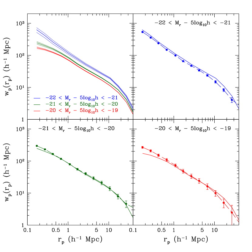
The discrepancy in the clustering of the faintest bin at small separations may be a result of numerical effects such as artificial disruption or halo misidentification in dense environments. A small deviation at the closest separations () is likely to have the same origin. Since the fraction of halos that are satellites decreases sharply at large halo masses (see Klypin et al., 2010), the model correlation functions of the brightest galaxies do not suffer from these effects. Further scrutiny is necessary to understand the origin of the effect and make more robust comparisons with observations.
6.5.1 Effect of scatter on the correlation function
Since only the brightest galaxies in the LV relation are affected by scatter, the obtained two-point correlation function of galaxies brighter than will be sensitive to the choice of scatter distribution. In the past few years, some studies of the correlation function of DM halos have suggested the scatter to be an essential ingredient in reproducing the observations (e.g., Tasitsiomi et al., 2004; Wetzel & White, 2010; Behroozi et al., 2010).
Figure 15 shows the galaxy autocorrelation function obtained for our model galaxies using the stochastic method described in Appendix A to perform HAM. Here we assume the same distribution described in Section 6.2.4, with below and above. The correlation amplitude of model galaxies fainter than is essentially unchanged compared to the monotonic assignment result shown in Figure 14. The clustering of the bright galaxies with shows a slight decrease at all separations except the smallest ones, and thus better agreement with the SDSS data. The amplitude decreased due to the fact that the same galaxies now get assigned to less massive halos on average, and these halos are less clustered. This is consistent with the upward shift in the average luminosity of the brightest galaxies in the LV relation (Figure 9). The correlation functions of galaxies in fainter bins are indistinguishable from those without scatter.

In summary, applying our physically motivated scatter model maintains (and even improves) the excellent agreement of the CDM+HAM model with the observed galaxy clustering. The clustering of the most massive and rare galaxies (those above ) will be more sensitive to the addition of scatter and the model used to implement it. Once other dominant sources of uncertainty in the simulations and observations are better understood, a robust test of the cosmological model could be done using these objects.
7 Comparison with other results
Our results are broadly consistent with Guo et al. (2010), who also use the abundance matching technique. Specifically, in their Figure 6 they show the stellar-mass – circular velocity relation. The theoretical velocities appear to be smaller than the observed circular velocities for . Although Guo et al. (2010) did not apply the necessary corrections discussed in our paper, they argue that inclusion of the cold baryon mass may bring the theory into agreement with the observations. As we show, indeed this is the case.
Incidentally, in the semi-analytic modeling paper (Guo et al., 2011) based on the Millennium-I and II simulations, the predicted angular correlation function of galaxies with is significantly too high compared with SDSS data, especially at separations less than about 1 Mpc. The authors attribute this to the fact that the large used in the Millennium simulations produced too many massive halos that in turn host too many pairs of galaxies in their subhalos.
Dutton et al. (2007) argue that the standard cosmological model with adiabatic contraction and standard concentrations fails to simultaneously reproduce the observed LV relation and the luminosity function for late-type galaxies. This conclusion is not compatible with our results. A number of assumptions made in Dutton et al. (2007) are either outdated or need corrections. For example, for their preferred model they use the “standard concentrations” of Bullock et al. (2001), which were based on a simulation with , although they attempted to rescale them to a cosmological model with the normalization . The normalization of the current CDM cosmological model is based on CMB and other data (e.g. Jarosik et al., 2010), which results in halo concentrations that are 30% lower than what Dutton et al. (2007) used in their preferred model. In turn, this reduces the dark matter circular velocities in the inner regions of halos by about 15%. Some of the necessary corrections were discussed by Dutton et al. (2007) and it was shown that they substantially improve the fit of the TF relation. However, the main difference is the treatment of the luminosity function. Dutton et al. (2007) use criteria obtained from SAMs to argue that a model with halo expansion is necessary to match the LF. We avoid such assumptions completely because our model reproduces the galaxy statistics automatically.
Gnedin et al. (2007) studied structural properties of spiral galaxies and compared them with theoretical predictions. They also used Bullock et al. (2001) high concentrations as the “standard” model. It was concluded that the theory has problems and that adiabatic contraction is the likely culprit. Another possible solution was to lower the halo concentrations. Indeed, when Gnedin et al. (2007) used concentrations for a model with as predicted by simple theoretical arguments, they found that the theory gives an acceptable fit to the data. The problem is that is too low. However, it seems that their analytical scaling with was not accurate enough: the concentrations actually used by Gnedin et al. (2007) are practically (within 3%) the same as what we find in -body simulations for the Bolshoi CDM model with (Klypin et al., 2010). In short, there seems to be no contradiction between our results and Gnedin et al. (2007) even when we consider models with standard adiabatic contraction. More definite conclusions require careful analysis and changes in the fraction of cold baryons among other things.
8 Discussion
In this paper we address one of the most difficult problems in cosmology: is the standard cosmological CDM model compatible with observations when it comes to the prediction of the abundance and properties of galaxies? Instead of focusing on traditional issues such as the zero-point and the slope of the Tully-Fisher relation for spiral galaxies, we work with a more generic luminosity-velocity (LV) relation: a correlation of galaxy luminosity with the circular velocity at a 10 kpc radius. We also investigate the (cold) baryonic mass - velocity relation, which following tradition we call the baryonic Tully-Fisher (BTF) relation, as well as the velocity function and the two-point autocorrelation function of galaxies. All these statistics encompass galaxies of different types - from dwarf galaxies to normal spirals to giant ellipticals. These statistics – in combination with the theoretical predictions of the cosmic microwave background and the abundance and properties of dark matter halos – are major tests for the validity of the CDM model.
We use the abundance matching technique to assign luminosities to halos predicted by cosmological simulations. We also use abundance matching to assign stellar and cold baryon masses. We find that all three statistics – the LV and BTF relations, and the velocity function – provide reasonably good fits to observations for galaxies ranging over 10 magnitudes in luminosity and for circular velocities from to . By construction, our models fit the observed luminosity and stellar mass functions. Since they are based on the Bolshoi simulation (Klypin et al., 2010), they also fit known properties of dark matter halos including the halo mass function and the dependence of halo concentration on mass. In addition, in this paper we show that halo abundance matching also yields the correct clustering properties of bright galaxies. In short, we have a model, that fits – at least on average – all the basic statistics of galaxies with considered at a 10 kpc scale.
Matching theory with observations requires a careful consideration of many different effects and application of different corrections. These effects were considered both for observations and for the theory. On the observational side, we compiled a representative sample of galaxies with measured circular velocities. Velocities were either asymptotic values (“flat part” of rotation curves) for spirals or measurements at kpc radius for S0s and Es. We do not use fits (such as power-laws) to the data but instead work directly with the distributions. We do not apply morphological corrections of the TF relation (e.g., differences between Sb and Sa galaxies) because those corrupt the bright end of the LV relation. Since the Tully-Fisher luminosities are corrected to face-on, we de-correct the magnitudes of galaxies for the effect of internal absorption to make them consistent with the measurement of the luminosity function.
For the theoretical predictions we try to make all the possible corrections to mimic the observational situation. For example, we do not use virial masses of halos because virial radii are too large compared with the typical distances at which rotational velocities of observed galaxies are measured. We do not assume a particular shape for the halo density profiles: they are measured directly in the simulations. The simulations required for this type of analysis should have a very high resolution so that subhalos are also resolved. This allows us to avoid using intermediate steps such as the Halo Occupation Distribution or the Conditional Luminosity Function, which are often applied to low-resolution simulations. The Bolshoi cosmological simulation (Klypin et al., 2010) provides high quality results resolving distinct halos and subhalos down to the completeness limit of .
The observations should be taken cautiously since each has a different degree of accuracy. The LV relation is the most accurate because it is easier to measure luminosities than to estimate stellar masses, which require additional modeling and assumptions. This is why we consider the LV relation as our prime target. The velocity function is the least reliable since observations are still at the very early stages. The completeness of the HIPASS VF is very uncertain. Just the fact that the detection limit is quoted at shows that the accuracy of the HI mass function is not very high. This is why we treat the results on the velocity function for as a “pass” for the theory in spite of some deviations such as at . More accurate treatment of these gas-rich galaxies may also change the situation: after all, changes in abundances and velocities by may (or may not) resolve the discrepancies.
It is more difficult to reconcile the theory and observations at smaller velocities. Indeed, at the formal disagreement is almost a factor of ten. This is the only serious problem that we find when matching galaxies with dark matter halos. A similar problem on somewhat smaller scales was reported by Tikhonov & Klypin (2009), who studied the population of dwarfs in the Mpc region centered on the Milky Way galaxy. Tikhonov et al. (2009) argue that Warm Dark matter may be the solution to the problem.
We introduce a simple scatter model that is well motivated and preserves the agreement with the LV relation and the correlation function of galaxies in the SDSS. The introduction of scatter has some complications. Observed deviations from the median relations seem to have a systematic component: early-type galaxies are systematically below the median LV relation and gas-rich spirals are above it. It seems likely that the LV relation – like the color-magnitude diagram – has a bimodal structure. In this case, no simple gaussian spread can explain the whole diagram. However uncertain, the spread must be explained. One approach might be to match halos separately to red and blue galaxies, for example using local density as well as luminosity. Ultimately it will be necessary to find the real source of the dynamical bimodality and to measure it observationally.
Although our CDM+HAM prescription makes simplifying assumptions regarding the distribution of baryons in DM halos, it yields results that are compatible with more detailed dynamical models. Our model predicts values that differ by less than 5% from Dutton et al. (2010b) for massive disk galaxies without halo contraction. Given that Dutton et al. (2010b) include a large set of observational constraints on the radial distribution of baryons, the consistency with our results is evidence of the robustness of our model666Dutton et al. (2010b) used LV relations to find that late- and early-type galaxies are best fitted by halo expansion and halo contraction (à la Gnedin et al. 2004), respectively. As mentioned above, we do see a systematic difference between early- and late-types in our assembled data sets that might be explained by some combination of differences in halo contraction and halo masses (Figures 4 and 11). However, given the observational uncertainties and the non-differentiation between early and late-types in our models, we cannot yet provide a precise interpretation of the bimodality..
Abundance matching is a very successful way to make predictions about how on average galaxies can inhabit dark matter halos. It gives up solving the most difficult and the most important problem: how galaxies form inside dark matter halos. It simply assumes that the stellar mass and luminosity monotonically (or possibly with some scatter) scale with the circular velocity. Bluntly speaking, it assumes that the maximum circular velocity of a halo determines the properties of the galaxy hosted by that halo. Remarkably, this can reproduce some basic environmental relations such as the morphology-density relation and the dependence of galaxy clustering on the luminosity of galaxies (e.g., Conroy et al., 2006) because of the correlation of environment with the average halo mass (Sheth et al., 2001; Sheth & Tormen, 2004). However, there are potential issues with abundance matching. It is not clear how it can explain dependencies on environment even if galaxies are selected with the same -band luminosity or the same stellar mass (Hogg et al., 2004; van der Wel, 2008). Modeling of the bimodality in the LV relation (the apparent differences between early and late type galaxies) is another problem to address. It will be interesting to see how much better the results will be from more sophisticated abundance matching including galaxy color and local density – as, e.g., in Tasitsiomi et al. (2004) – and from semi-analytic modeling based on the Bolshoi simulation. This work is in progress.
Disk formation and semi-analytic models still struggle to simultaneously reproduce the TF relation (a subset of the LV relation) and the abundance of galaxies (e.g., Benson et al., 2003; Monaco et al., 2007; Benson & Bower, 2010). In this paper we have shown that our model is successful at this task. Simultaneously reproducing the luminosity function and the LV relation depends critically on implementing each of the steps in Section 5 to obtain the properties of the galaxies that inhabit CDM halos. For example, Figure 8 shows how assuming an incorrect value for the baryon fraction (as in Mo et al. (1998)) can lead to an LV relation that is in striking disagreement with the observations. In the more recent semi-analytic model of Benson & Bower (2010) the circular velocities of galaxies are larger than observed at any luminosity. This may be explained by the fact that their baryon fraction is about larger than ours for Milky Way-mass galaxies and about an order of magnitude larger than our result for the most massive ellipticals as well as dwarfs. Our model shows that galaxies with masses larger that the Milky Way have circular velocities that are extremely sensitive to the baryon content within their optical radius which may explain why SAMs overpredict the circular velocity.
Previous works based on abundance matching were successful at reproducing the statistics of the integrated properties of galaxies (such as clustering as a function of luminosity and redshift) but made no attempt to include their internal and baryonic structure (e.g., Kravtsov et al., 2004; Conroy et al., 2006; Wetzel & White, 2010; Behroozi et al., 2010; Guo et al., 2010). In this paper we show that making robust dynamical corrections to the structure of halos obtained in simulations gives the correct galaxy scaling relations. These corrections include adding the cold baryonic component and measuring at . Previous studies using HAM could not include these corrections partly because simulations lacked the large dynamic range necessary to form the largest halos and resolve substructure adequately. The large box size and very high resolution of the Bolshoi simulation makes it possible to obtain good statistics of even the largest clusters and resolve the structure of dwarf halos.
9 Conclusions
Here is a short summary of our results:
-
•
In combination with previous results, we conclude that the standard CDM model in conjunction with halo abundance matching can simultaneously fit reasonably well the main global statistics of galaxies: the luminosity function, the stellar mass function, the Luminosity-Velocity relation, the baryonic Tully-Fisher relation, the abundance of galaxies with circular velocities , as well as the clustering properties of bright galaxies as a function of luminosity.
-
•
There are systematic deviations in the LV relation with S0 and elliptical galaxies located about 1 magnitude below late types in the LV relation. Massive early types contain less baryonic mass than late types at the same circular velocity.
-
•
The range of the effect of contraction of the DM halos due to baryon infall brackets the observations. The LV relation shows preference for a model with moderate contraction, as predicted by Gnedin et al. (2004). This result is compatible with the observed velocity function of galaxies.
-
•
There seems to be an overabundance of model galaxies by a factor of compared to observed dwarf galaxies with . This is a serious problem for the CDM model: galaxies with these circular velocities cannot be affected much by “normal” physical processes (e.g., supernovae feedback or reionization of the Universe) proposed for the solution of the satellite problem at . However, the observational results on the abundance of dwarf galaxies still need to be improved.
-
•
Including scatter in luminosity at fixed using our physically motivated scatter model maintains the agreement of the model LV relation with observations.
-
•
The correlation function of the model Bolshoi galaxies matches very well the observations of bright galaxies. The agreement improves when implementing our scatter prescription for all but the brightest galaxies, where a better understanding of the uncertainties is necessary to make a fair test of CDM using halo abundance matching.
Appendix A Halo abundance matching including stochastic scatter
To perform halo abundance matching while including scatter in luminosity as a function of circular velocity we perform the following procedure. For brevity, wherever we use we refer to .
-
1.
Start with the monotonic assignment described in Section 5: Order the list of DM halos from largest to smallest . Using the integral LF, solve for the unique luminosities of the galaxies that have the same number densities as the DM halos in Bolshoi. This matching gives the monotonic relation .
-
2.
For the halo with the largest , draw a luminosity value at random from a Gaussian distribution of width centered at a point 1- brighter than the value of for that halo. Mathematically, this is equivalent to , where is a random realization of a Gaussian probability distribution with standard deviation centered at zero.
-
3.
If the randomly drawn is brighter than the brightest galaxy in the LF, another draw is performed and the process is repeated until a suitable value is found.
-
4.
The random is compared to the list of available values in the list. The closest available value becomes the luminosity of that halo. If the value is already taken, another random draw is performed until an available one is found. This luminosity value is flagged to prevent it from being used again for another halo. This step ensures that the observed luminosity function is preserved by only assigning each luminosity once.
-
5.
In order to avoid having unassigned values of in the list on the bright tail of the distribution, we check whether there is any unassigned luminosity which is more than 3- brighter than . If such unassigned value exists, the next halo in the list is assigned to it. Since we are stepping along the list of luminosities as we assign them, the process is intrinsically asymmetric and there will always be some leftover values that get assigned in this step. The offset used in step 1 ensures that these make up only a few percent of the sample.
-
6.
Repeat steps 2-5 for each halo in the ordered list until the 3- faint tail of the Gaussian for a given halo reaches the completeness limit of the sample as defined in Section 3. The procedure is stopped at this point to prevent placing a hard constraint on the faint end of the LF where it is most uncertain. The faintest halos (up to 0.5 magnitudes brighter than the cutoff) are removed from the sample to insure the preservation of the LF throughout.
In spite of the fact that a constant Gaussian distribution is used in the algorithm, the final distribution of for a given circular velocity is not a Gaussian and the width of the relation is not constant. This happens because of the asymmetry in the distribution of the galaxies: there are always more galaxies with smaller luminosities than with larger ones. Thus, the distribution and the spread of the final relation are the result of a convolution of a Gaussian distribution with the luminosity function.
The effect of the asymmetry of the LF is more pronounced for the brightest galaxies in the sample and accounts for the small shift in the median compared to the monotonic assignment. The algorithm also gives a natural narrowing of the distribution of luminosities as increases. This occurs because in the exponential tail of the LF the number of available values changes rapidly across the width of the Gaussian. Increasingly fewer available values on the bright side of the median force the selection of most values to take place in a narrower interval on the faint side.
Since our assignment method reduces the width of the obtained distribution of luminosities, we choose the input value . This yields a distribution with below and gradually decreasing to above .
Figure 16 shows the distribution of luminosities in four bins of circular velocity, . Below , galaxies show a near-normal distribution that is centered very close to the values obtained from the monotonic assignment without scatter. For the distributions get progressively more skewed as galaxies move from the bright to the faint tail. The spread of the distribution of luminosities increases with : the widths are , , and for the bins centered at , , and respectively.
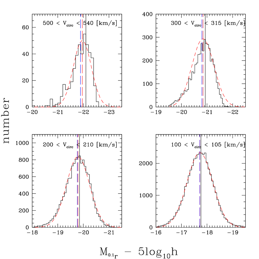
Figure 17 shows the LV relation obtained with the scatter model of Behroozi et al. (2010) in the case of constant scatter (left panel) as well as assuming the same variable width used in our model: for declining to for larger . Evidently, the median of the distribution in luminosity stays relatively unchanged only when forcing a small scatter width at the bright end. Even when we impose the same variable width used in the stochastic HAM scheme, the resulting spread is too large for the brightest galaxies.
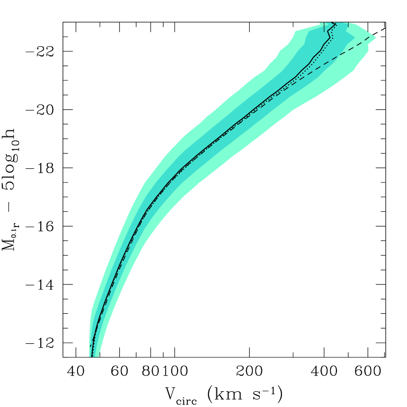
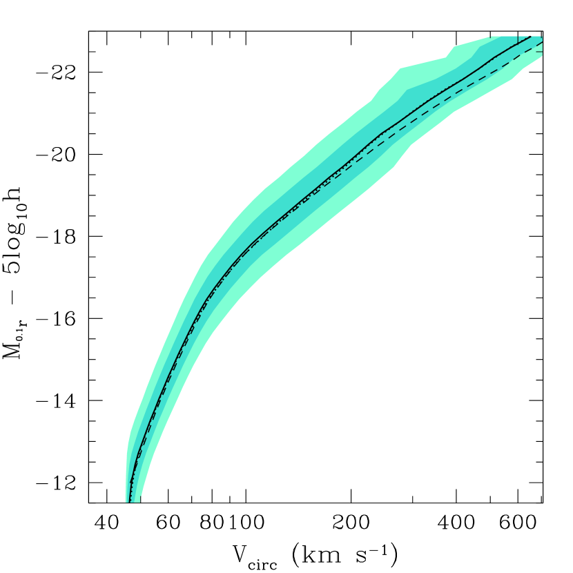
Appendix B Early-type data
Table 1 gives some of the properties of our early-type sample along with the source of data for each galaxy.
| Name | Type | probe | ref. | ||||||||||||
|---|---|---|---|---|---|---|---|---|---|---|---|---|---|---|---|
| NGC 4889 | E | 0.16 | 11.87 | 520 | 60 | 50 | — | — | — | — | — | — | stars | T+07 | |
| NGC 4874 | E | 0.16 | 11.65 | 500 | 30 | 50 | 510 | 60 | 70 | — | — | — | stars | T+07 | |
| NGC 0315 | E | 0.25 | 11.66 | 520 | 10 | 5 | 530 | 30 | 10 | 550 | 35 | 20 | stars | K+00 | |
| NGC 1316 | S0 | 0.19 | 11.46 | 381 | 29 | 29 | 466 | 52 | 52 | 361 | 49 | 49 | X-ray | NM09 | |
| NGC 4839 | E | 0.15 | 11.52 | 385 | 65 | 30 | 400 | 80 | 50 | 425 | 105 | 70 | stars | T+07 | |
| NGC 0057 | E | 0.19 | 11.56 | 491 | 20 | 49 | 494 | 19 | 52 | 495 | 22 | 52 | X-ray | O+07 | |
| NGC 4555 | E | 0.21 | 11.50 | 614 | 58 | 62 | 606 | 61 | 66 | 598 | 63 | 74 | X-ray | OP04 | |
| NGC 4952 | E | 0.19 | 11.37 | 405 | 10 | 15 | 435 | 20 | 30 | 455 | 25 | 45 | stars | T+07 | |
| NGC 6407 | E/S0 | 0.26 | 11.51 | 445 | 25 | 35 | 450 | 50 | 40 | 460 | 60 | 60 | stars | MB01 | |
| NGC 4472 | E | 0.12 | 11.41 | 415 | 40 | 40 | — | — | — | — | — | — | stars | MB01 | |
| NGC 7626 | E | 0.20 | 11.41 | 420 | 9 | 10 | 410 | 15 | 15 | 390 | 20 | 15 | stars | K+00 | |
| NGC 5044 | E | 0.27 | 11.31 | 273 | 17 | 17 | 328 | 11 | 11 | 365 | 13 | 13 | X-ray | NM09 | |
| NGC 4486 | E | 0.16 | 11.31 | 503 | 47 | 34 | — | — | — | — | — | — | GCs | M+11 | |
| NGC 3923 | E | 0.43 | 11.26 | 365 | 28 | 28 | 324 | 40 | 40 | 324 | 40 | 40 | X-ray | NM09 | |
| NGC 4816 | E/S0 | 0.23 | 11.19 | 300 | 45 | 40 | 300 | 50 | 40 | 310 | 50 | 40 | stars | T+07 | |
| NGC 1395 | E | 0.17 | 11.26 | 374 | 17 | 17 | — | — | — | — | — | — | X-ray | NM09 | |
| NGC 4944 | S0 | 0.32 | 11.19 | 275 | 2 | 2 | 280 | 2 | 2 | 280 | 2 | 2 | stars | T+07 | |
| NGC 4382 | S0/a | 0.16 | 11.12 | 260 | 19 | 19 | 260 | 19 | 19 | 198 | 51 | 51 | X-ray | NM09 | |
| NGC 4649 | E | 0.16 | 11.27 | 425 | 10 | 10 | 436 | 21 | 22 | 444 | 35 | 37 | X-ray | HB10 | |
| NGC 4374 | E | 0.12 | 11.26 | 382 | 20 | 20 | 386 | 20 | 20 | 393 | 20 | 20 | PNe | N+11 | |
| NGC 4827 | E/S0 | 0.23 | 11.20 | 350 | 50 | 30 | — | — | — | — | — | — | stars | T+07 | |
| NGC 0128 | S0 | 0.20 | 11.18 | 370 | 14 | 14 | 361 | 15 | 15 | — | — | — | stars | W+09 | |
| IC 1459 | E | 0.21 | 11.26 | 338 | 53 | 53 | 258 | 53 | 53 | 282 | 45 | 45 | X-ray | NM09 | |
| NGC 4957 | E | 0.19 | 11.21 | 325 | 2 | 2 | 310 | 10 | 2 | 295 | 15 | 2 | stars | T+07 | |
| NGC 4261 | E | 0.20 | 11.20 | 362 | 27 | 29 | 338 | 27 | 29 | 332 | 30 | 33 | X-ray | HB10 | |
| NGC 6703 | E/S0 | 0.20 | 11.11 | 220 | 20 | 15 | — | — | — | — | — | — | stars | K+00 | |
| NGC 3665 | S0 | 0.23 | 11.13 | 423 | 52 | 52 | 404 | 32 | 32 | 404 | 32 | 32 | X-ray | NM09 | |
| NGC 5846 | E | 0.24 | 11.19 | 340 | 5 | 5 | — | — | — | — | — | — | stars | K+00 | |
| NGC 4908 | E | 0.15 | 11.19 | 320 | 40 | 40 | — | — | — | — | — | — | stars | T+07 | |
| NGC 0720 | E | 0.18 | 11.18 | 317 | 12 | 13 | 323 | 13 | 13 | 330 | 11 | 12 | X-ray | HB10 | |
| NGC 7796 | E | 0.20 | 11.15 | 308 | 46 | 26 | 305 | 37 | 28 | 297 | 35 | 26 | X-ray | O+07 | |
| NGC 4365 | E | 0.18 | 11.15 | 333 | 26 | 26 | 333 | 26 | 26 | — | — | — | X-ray | NM09 | |
| NGC 3607 | E/S0 | 0.20 | 11.07 | 278 | 28 | 28 | 278 | 28 | 28 | 265 | 28 | 28 | X-ray | NM09 | |
| NGC 1399 | E | 0.19 | 11.11 | 430 | 25 | 30 | — | — | — | — | — | — | stars | K+00 | |
| NGC 3585 | E | 0.22 | 10.99 | 295 | 46 | 46 | — | — | — | — | — | — | X-ray | NM09 | |
| NGC 2974 | E | 0.20 | 11.06 | 304 | 10 | 10 | — | — | — | — | — | — | gas | W+08 | |
| NGC 5084 | S0 | 0.21 | 11.05 | 282 | 8 | 8 | — | — | — | — | — | — | stars | W+09 | |
| NGC 6771 | S0/a | 0.17 | 10.92 | 340 | 18 | 18 | 331 | 18 | 18 | 320 | 23 | 23 | stars | W+09 | |
| NGC 4807 | E/S0 | 0.23 | 10.99 | 295 | 30 | 15 | — | — | — | — | — | — | stars | T+07 | |
| NGC 4931 | S0 | 0.23 | 11.02 | 280 | 5 | 15 | 275 | 10 | 25 | 270 | 15 | 30 | stars | T+07 | |
| NGC 0821 | E | 0.21 | 10.88 | 182 | 13 | 13 | — | — | — | — | — | — | stars | FG10 | |
| NGC 1332 | E/S0 | 0.22 | 10.94 | 291 | 9 | 10 | 291 | 9 | 10 | 291 | 9 | 10 | X-ray | HB10 | |
| IC 0843 | S0 | 0.19 | 10.83 | 380 | 10 | 5 | 340 | 20 | 10 | 320 | 25 | 15 | stars | T+07 | |
| ESO151-G004 | S0 | 0.26 | 11.10 | 291 | 19 | 19 | 308 | 19 | 19 | 295 | 25 | 25 | stars | W+09 | |
| NGC 4494 | E | 0.17 | 10.77 | 198 | 10 | 10 | 188 | 14 | 14 | 184 | 18 | 18 | PNe | N+09 | |
| NGC 4869 | E | 0.15 | 10.91 | 280 | 50 | 30 | — | — | — | — | — | — | stars | T+07 | |
| NGC 4636 | E | 0.17 | 10.85 | 430 | 16 | 16 | 491 | 22 | 22 | 538 | 29 | 29 | X-ray | NM09 | |
| NGC 1032 | S0/a | 0.21 | 10.82 | 270 | 20 | 20 | — | — | — | — | — | — | stars | W+09 | |
| NGC 4697 | E | 0.18 | 10.73 | 235 | 15 | 10 | 234 | 17 | 19 | 231 | 23 | 26 | PNe | dL+08 | |
| IC 4045 | E | 0.15 | 10.85 | 390 | 40 | 30 | — | — | — | — | — | — | stars | T+07 | |
| NGC 3203 | S0/a | 0.25 | 10.47 | 229 | 7 | 7 | — | — | — | — | — | — | stars | W+09 | |
| NGC 3379 | E | 0.11 | 10.69 | 206 | 31 | 13 | 192 | 42 | 19 | 181 | 48 | 22 | PNe | dL+09 | |
| NGC 3957 | S0/a | 0.20 | 10.38 | 199 | 13 | 13 | — | — | — | — | — | — | stars | W+09 | |
| NGC 4710 | S0/a | 0.21 | 10.12 | 182 | 10 | 10 | — | — | — | — | — | — | stars | W+09 | |
| NGC 4469 | S0/a | 0.17 | 10.22 | 182 | 13 | 13 | — | — | — | — | — | — | stars | W+09 |
Note. — The galaxies are sorted by absolute magnitude , which is corrected for Galactic extinction; the quoted errors include the statistical uncertainties in distance and photometry. The stellar masses are based on colors, and correspond to a Chabrier IMF (see text). Circular velocities , , and are measured at 10, 15, and 20 kpc, respectively, and are in units of km s-1. References: dL+08: de Lorenzi et al. (2008); dL+09: de Lorenzi et al. (2009); FG10: Forestell & Gebhardt (2010); HB10: Humphrey & Buote (2010); K+00: Kronawitter et al. (2000); M+11: Murphy et al. (2011); MB01: Magorrian & Ballantyne (2001); N+09: Napolitano et al. (2009); N+11: Napolitano et al. (2011); NM09: Nagino & Matsushita (2009); OP04: O’Sullivan & Ponman (2004); O+07: O’Sullivan et al. (2007); T+07: Thomas et al. (2007); W+08: Weijmans et al. (2008); W+09: Williams et al. (2009).
References
- Baldry et al. (2008) Baldry, I. K., Glazebrook, K., & Driver, S. P. 2008, MNRAS, 388, 945
- Behroozi et al. (2010) Behroozi, P. S., Conroy, C., & Wechsler, R. H. 2010, ApJ, 717, 379
- Bell & de Jong (2001) Bell, E. F., & de Jong, R. S. 2001, ApJ, 550, 212
- Bell et al. (2003) Bell, E. F., McIntosh, D. H., Katz, N., & Weinberg, M. D. 2003, ApJS, 149, 289
- Benson et al. (2003) Benson, A. J., Bower, R. G., Frenk, C. S., Lacey, C. G., Baugh, C. M., & Cole, S. 2003, ApJ, 599, 38
- Benson & Bower (2010) Benson, A. J., & Bower, R. G. 2010, arXiv:1003.0011
- Blanton et al. (2003a) Blanton, M. R., et al. 2003a, ApJ, 594, 186
- Blanton et al. (2003b) Blanton, M. R., et al. 2003b, AJ, 125, 2348
- Blanton et al. (2005) Blanton, M. R., Lupton, R. H., Schlegel, D. J., Strauss, M. A., Brinkmann, J., Fukugita, M., & Loveday, J. 2005, ApJ, 631, 208
- Blanton & Roweis (2007) Blanton, M. R., & Roweis, S. 2007, AJ, 133, 734
- Blanton et al. (2008) Blanton, M. R., Geha, M., & West, A. A. 2008, ApJ, 682, 861
- Blumenthal et al. (1986) Blumenthal, G. R., Faber, S. M., Flores, R., & Primack, J. R. 1986, ApJ, 301, 27
- Boylan-Kolchin et al. (2009) Boylan-Kolchin, M., Springel, V., White, S. D. M., Jenkins, A., & Lemson, G. 2009, MNRAS, 398, 1150 (MS-II)
- Bullock et al. (2000) Bullock, J. S., Kravtsov, A. V., & Weinberg, D. H. 2000, ApJ, 539, 517
- Bullock et al. (2001) Bullock, J. S., Kolatt, T. S., Sigad, Y., Somerville, R. S., Kravtsov, A. V., Klypin, A. A., Primack, J. R., & Dekel, A. 2001, MNRAS, 321, 559
- Chae (2010) Chae, K.-H. 2010, MNRAS, 402, 2031
- Chabrier (2003) Chabrier, G. 2003, PASP, 115, 763
- Cole et al. (1994) Cole, S., Aragon-Salamanca, A., Frenk, C. S., Navarro, J. F., & Zepf, S. E. 1994, MNRAS, 271, 781
- Cole et al. (2000) Cole, S., Lacey, C. G., Baugh, C. M., & Frenk, C. S. 2000, MNRAS, 319, 168
- Conroy et al. (2006) Conroy, C., Wechsler, R. H., & Kravtsov, A. V. 2006, ApJ, 647, 201
- Conroy & Wechsler (2009) Conroy, C., & Wechsler, R. H. 2009, ApJ, 696, 620
- Courteau (1997) Courteau, S. 1997, AJ, 114, 2402
- Courteau et al. (2007) Courteau, S., Dutton, A. A., van den Bosch, F. C., MacArthur, L. A., Dekel, A., McIntosh, D. H., & Dale, D. A. 2007, ApJ, 671, 203
- de Blok & McGaugh (1997) de Blok, W. J. G., & McGaugh, S. S. 1997, MNRAS, 290, 533
- de Blok (2010) de Blok, W. J. G. 2010, Advances in Astronomy, 2010
- Dehnen & Binney (1998) Dehnen, W., & Binney, J. 1998, MNRAS, 294, 429
- de Lorenzi et al. (2008) de Lorenzi, F., Gerhard, O., Saglia, R. P., Sambhus, N., Debattista, V. P., Pannella, M., & Méndez, R. H. 2008, MNRAS, 385, 1729
- de Lorenzi et al. (2009) de Lorenzi, F., et al. 2009, MNRAS, 395, 76
- de Vaucouleurs et al. (1991) de Vaucouleurs, G., de Vaucouleurs, A., Corwin, H. G., Jr., Buta, R. J., Paturel, G., & Fouque, P. 1991, Volume 1-3, XII, 2069 pp. 7 figs.. Springer-Verlag Berlin Heidelberg New York
- Duffy et al. (2010) Duffy, A. R., Schaye, J., Kay, S. T., Dalla Vecchia, C., Battye, R. A., & Booth, C. M. 2010, arXiv:1001.3447
- Dunkley et al. (2009) Dunkley, J., et al. 2009, ApJS, 180, 306
- Dutton et al. (2007) Dutton, A. A., van den Bosch, F. C., Dekel, A., & Courteau, S. 2007, ApJ, 654, 27
- Dutton & van den Bosch (2009) Dutton, A. A., & van den Bosch, F. C. 2009, MNRAS, 396, 141
- Dutton et al. (2010a) Dutton, A. A., Conroy, C., van den Bosch, F. C., Prada, F., & More, S. 2010a, MNRAS, 407, 2
- Dutton et al. (2010b) Dutton, A. A., et al. 2010b, arXiv:1012.5859
- Einasto (1965) Einasto, J. 1965, Trudy Inst. Astrofiz. Alma-Ata, 5, 87
- Eke et al. (2001) Eke, V. R., Navarro, J. F., & Steinmetz, M. 2001, ApJ, 554, 114
- Faber & Jackson (1976) Faber, S. M., & Jackson, R. E. 1976, ApJ, 204, 668
- Flores & Primack (1994) Flores, R. A., & Primack, J. R. 1996, ApJ, 457, L5
- Forestell & Gebhardt (2010) Forestell, A., & Gebhardt, K. 2010, ApJ, in press, arXiv:0803.3626
- Fukugita et al. (1998) Fukugita, M., Hogan, C. J., & Peebles, P. J. E. 1998, ApJ, 503, 518
- Fukugita & Peebles (2004) Fukugita, M., & Peebles, P. J. E. 2004, ApJ, 616, 643
- Geha et al. (2006) Geha, M., Blanton, M. R., Masjedi, M., & West, A. A. 2006, ApJ, 653, 240
- Gnedin et al. (2004) Gnedin, O. Y., Kravtsov, A. V., Klypin, A. A., & Nagai, D. 2004, ApJ, 616, 16
- Gnedin et al. (2007) Gnedin, O. Y., Weinberg, D. H., Pizagno, J., Prada, F., & Rix, H.-W. 2007, ApJ, 671, 1115
- Gonzalez et al. (2000) Gonzalez, A. H., Williams, K. A., Bullock, J. S., Kolatt, T. S., & Primack, J. R. 2000, ApJ, 528, 145
- Gottloeber & Klypin (2008) Gottloeber, S., & Klypin, A. 2008, in ”High Performance Computing in Science and Engineering Garching/Munich 2007”, Eds. S. Wagner et al, Springer, Berlin 2008 (arXiv:0803.4343)
- Governato et al. (2007) Governato, F., Willman, B., Mayer, L., Brooks, A., Stinson, G., Valenzuela, O., Wadsley, J., & Quinn, T. 2007, MNRAS, 374, 1479
- Governato et al. (2010) Governato, F., et al. 2010, Nature, 463, 203
- Graham et al. (2005) Graham, A. W., Driver, S. P., Petrosian, V., Conselice, C. J., Bershady, M. A., Crawford, S. M., & Goto, T. 2005, AJ, 130, 1535
- Graham et al. (2006) Graham, A. W., Merritt, D., Moore, B., Diemand, J., & Terzić, B. 2006, AJ, 132, 2701
- Guedes et al. (2011) Guedes, J., Calligari, S., Madau, P., & Mayer, L. 2011, arXiv:1103.6030
- Guo et al. (2010) Guo, Q., White, S., Li, C., & Boylan-Kolchin, M. 2010, MNRAS, 367
- Guo et al. (2011) Guo, Q., et al. 2011, MNRAS, 413, 101
- Hill et al. (2010) Hill, D. T., Driver, S. P., Cameron, E., Cross, N., Liske, J., & Robotham, A. 2010, arXiv:1002.3788
- Hinshaw et al. (2009) Hinshaw, G., et al. 2009, ApJS, 180, 225
- Hogg et al. (2004) Hogg, D. W., et al. 2004, ApJ, 601, L29
- Humphrey & Buote (2010) Humphrey, P. J., & Buote, D. A. 2010, MNRAS, 403, 2143
- Jarosik et al. (2010) Jarosik, N., et al. 2010, arXiv:1001.4744
- Jensen et al. (2003) Jensen, J. B., Tonry, J. L., Barris, B. J., Thompson, R. I., Liu, M. C., Rieke, M. J., Ajhar, E. A., & Blakeslee, J. P. 2003, ApJ, 583, 712
- Kauffmann et al. (1993) Kauffmann, G., White, S. D. M., & Guiderdoni, B. 1993, MNRAS, 264, 201
- Klypin & Holtzman (1997) Klypin, A., & Holtzman, J. 1997, arXiv:astro-ph/9712217
- Klypin et al. (1999) Klypin, A., Gottlöber, S., Kravtsov, A. V., & Khokhlov, A. M. 1999, ApJ, 516, 530
- Klypin et al. (2001) Klypin, A., Kravtsov, A. V., Bullock, J. S., & Primack, J. R. 2001, ApJ, 554, 903
- Klypin et al. (2002) Klypin, A., Zhao, H., & Somerville, R. S. 2002, ApJ, 573, 597
- Klypin et al. (2009) Klypin, A., Valenzuela, O., Colín, P., & Quinn, T. 2009, MNRAS, 398, 1027
- Klypin et al. (2010) Klypin, A., Trujillo-Gomez, S., & Primack, J. 2010, arXiv:1002.3660
- Kochanek & White (2001) Kochanek, C. S., & White, M. 2001, ApJ, 559, 531
- Komatsu et al. (2009) Komatsu, E., et al. 2009, ApJS, 180, 330
- Komatsu et al. (2010) Komatsu, E., et al. 2010, arXiv:1001.4538
- Kravtsov et al. (1997) Kravtsov, A. V., Klypin, A. A., & Khokhlov, A. M. 1997, ApJS, 111, 73
- Kravtsov (1999) Kravtsov, A. V. 1999, Ph.D. Thesis
- Kravtsov et al. (2004) Kravtsov, A. V., Berlind, A. A., Wechsler, R. H., Klypin, A. A., Gottlöber, S., Allgood, B., & Primack, J. R. 2004, ApJ, 609, 35
- Kronawitter et al. (2000) Kronawitter, A., Saglia, R. P., Gerhard, O., & Bender, R. 2000, A&AS, 144, 53
- Lauer et al. (2007) Lauer, T. R., et al. 2007, ApJ, 662, 808
- Leroy et al. (2008) Leroy, A. K., Walter, F., Brinks, E., Bigiel, F., de Blok, W. J. G., Madore, B., & Thornley, M. D. 2008, AJ, 136, 2782
- Li & White (2009) Li, C., & White, S. D. M. 2009, MNRAS, 398, 2177
- Lupton (2005) Lupton, R. 2005, http://www.sdss.org/dr7/algorithms/sdssUBVRITransform.html#Lupton2005
- Macciò et al. (2010) Macciò, A. V., Kang, X., Fontanot, F., Somerville, R. S., Koposov, S., & Monaco, P. 2010, MNRAS, 402, 1995
- Magorrian & Ballantyne (2001) Magorrian, J., & Ballantyne, D. 2001, MNRAS, 322, 702
- Maller et al. (2009) Maller, A. H., Berlind, A. A., Blanton, M. R., & Hogg, D. W. 2009, ApJ, 691, 394
- Mandelbaum et al. (2006) Mandelbaum, R., Seljak, U., Kauffmann, G., Hirata, C. M., & Brinkmann, J. 2006, MNRAS, 368, 715
- Maraston (2005) Maraston, C. 2005, MNRAS, 362, 799
- Masters et al. (2008) Masters, K. L., Springob, C. M., & Huchra, J. P. 2008, AJ, 135, 1738
- McGaugh et al. (2000) McGaugh, S. S., Schombert, J. M., Bothun, G. D., & de Blok, W. J. G. 2000, ApJ, 533, L99
- McGaugh (2005) McGaugh, S. S. 2005, ApJ, 632, 859
- McGaugh et al. (2010) McGaugh, S. S., Schombert, J. M., de Blok, W. J. G., & Zagursky, M. J. 2010, ApJ, 708, L14
- Mo et al. (1998) Mo, H. J., Mao, S., & White, S. D. M. 1998, MNRAS, 295, 319
- Monaco et al. (2007) Monaco, P., Fontanot, F., & Taffoni, G. 2007, MNRAS, 375, 1189
- Montero-Dorta & Prada (2009) Montero-Dorta, A. D., & Prada, F. 2009, MNRAS, 399, 1106
- Moore (1994) Moore, B. 1994, Nature, 370, 629
- Moore et al. (1999) Moore, B., Ghigna, S., Governato, F., Lake, G., Quinn, T., Stadel, J., & Tozzi, P. 1999, ApJ, 524, L19
- Murphy et al. (2011) Murphy, J. D., Gebhardt, K., & Adams, J. J. 2011, ApJ, 729, 129
- Nagai & Kravtsov (2005) Nagai, D., & Kravtsov, A. V. 2005, ApJ, 618, 557
- Nagino & Matsushita (2009) Nagino, R., & Matsushita, K. 2009, A&A, 501, 157
- Napolitano et al. (2009) Napolitano, N. R., et al. 2009, MNRAS, 393, 329
- Napolitano et al. (2010) Napolitano, N. R., Romanowsky, A. J., & Tortora, C. 2010, MNRAS, 405, 2351
- Napolitano et al. (2011) Napolitano, N. R., et al. 2011, MNRAS, 411, 2035
- Navarro et al. (1997) Navarro, J. F., Frenk, C. S., & White, S. D. M. 1997, ApJ, 490, 493
- Navarro & Steinmetz (2000) Navarro, J. F., & Steinmetz, M. 2000, ApJ, 538, 477
- Navarro et al. (2004) Navarro, J. F., et al. 2004, MNRAS, 349, 1039
- O’Sullivan & Ponman (2004) O’Sullivan, E., & Ponman, T. J. 2004, MNRAS, 354, 935
- O’Sullivan et al. (2007) O’Sullivan, E., Sanderson, A. J. R., & Ponman, T. J. 2007, MNRAS, 380, 1409
- Paturel et al. (2003) Paturel, G., Petit, C., Prugniel, P., Theureau, G., Rousseau, J., Brouty, M., Dubois, P., & Cambrésy, L. 2003, A&A, 412, 45
- Peletier et al. (1990) Peletier, R. F., Davies, R. L., Illingworth, G. D., Davis, L. E., & Cawson, M. 1990, AJ, 100, 1091
- Pizagno et al. (2007) Pizagno, J., et al. 2007, AJ, 134, 945
- Prada et al. (2011) Prada, F., Klypin, A. A., Cuesta, A. J., Betancort-Rijo, J. E., & Primack, J. 2011, arXiv:1104.5130
- Primack (2009) Primack, J. R. 2009, New Journal of Physics, 11, 105029
- Romanowsky et al. (2003) Romanowsky, A. J., Douglas, N. G., Arnaboldi, M., Kuijken, K., Merrifield, M. R., Napolitano, N. R., Capaccioli, M., & Freeman, K. C. 2003, Science, 301, 1696
- Rozo et al. (2009) Rozo, E., et al. 2009, ApJ, 699, 768
- Sakai et al. (2000) Sakai, S., et al. 2000, ApJ, 529, 698
- Schulz et al. (2010) Schulz, A. E., Mandelbaum, R., & Padmanabhan, N. 2010, MNRAS, 408, 1463
- Sheth et al. (2001) Sheth, R. K., Mo, H. J., & Tormen, G. 2001, MNRAS, 323, 1
- Sheth & Tormen (2004) Sheth, R. K., & Tormen, G. 2004, MNRAS, 350, 1385
- Somerville & Primack (1999) Somerville, R. S., & Primack, J. R. 1999, MNRAS, 310, 1087
- Springel et al. (2005) Springel, V., et al. 2005, Nature, 435, 629 (MS-I)
- Springob et al. (2007) Springob, C. M., Masters, K. L., Haynes, M. P., Giovanelli, R., & Marinoni, C. 2007, ApJS, 172, 599
- Stark et al. (2009) Stark, D. V., McGaugh, S. S., & Swaters, R. A. 2009, AJ, 138, 392
- Strauss et al. (2002) Strauss, M. A., et al. 2002, AJ, 124, 1810
- Tasitsiomi et al. (2004) Tasitsiomi, A., Kravtsov, A. V., Wechsler, R. H., & Primack, J. R. 2004, ApJ, 614, 533
- Thomas et al. (2007) Thomas, J., Saglia, R. P., Bender, R., Thomas, D., Gebhardt, K., Magorrian, J., Corsini, E. M., & Wegner, G. 2007, MNRAS, 382, 657
- Tikhonov & Klypin (2009) Tikhonov, A. V., & Klypin, A. 2009, MNRAS, 395, 1915
- Tikhonov et al. (2009) Tikhonov, A. V., Gottlöber, S., Yepes, G., & Hoffman, Y. 2009, MNRAS, 399, 1611
- Tissera et al. (2009) Tissera, P. B., White, S. D. M., Pedrosa, S., & Scannapieco, C. 2009, arXiv:0911.2316
- Tortora et al. (2010) Tortora, C., Napolitano, N. R., Romanowsky, A. J., & Jetzer, P. 2010, ApJ, 721, L1
- Tully & Fisher (1977) Tully, R. B., & Fisher, J. R. 1977, A&A, 54, 661
- Tully et al. (1998) Tully, R. B., Pierce, M. J., Huang, J.-S., Saunders, W., Verheijen, M. A. W., & Witchalls, P. L. 1998, AJ, 115, 2264
- Vale & Ostriker (2004) Vale, A., & Ostriker, J. P. 2004, MNRAS, 353, 189
- Valenzuela et al. (2007) Valenzuela, O., Rhee, G., Klypin, A., Governato, F., Stinson, G., Quinn, T., & Wadsley, J. 2007, ApJ, 657, 773
- Verheijen (2001) Verheijen, M. A. W. 2001, ApJ, 563, 694
- van der Wel (2008) van der Wel, A. 2008, ApJ, 675, L13
- Walter et al. (2008) Walter, F., Brinks, E., de Blok, W. J. G., Bigiel, F., Kennicutt, R. C., Thornley, M. D., & Leroy, A. 2008, AJ, 136, 2563
- Weijmans et al. (2008) Weijmans, A.-M., Krajnović, D., van de Ven, G., Oosterloo, T. A., Morganti, R., & de Zeeuw, P. T. 2008, MNRAS, 383, 1343
- Wetzel & White (2010) Wetzel, A. R., & White, M. 2010, MNRAS, 403, 1072
- Widrow & Dubinski (2005) Widrow, L. M., & Dubinski, J. 2005, ApJ, 631, 838
- Williams et al. (2009) Williams, M. J., Bureau, M., & Cappellari, M. 2009, MNRAS, 400, 1665
- Williams et al. (2010) Williams, M. J., Bureau, M., & Cappellari, M. 2010, MNRAS, 409, 1330
- Willman et al. (2004) Willman, B., Governato, F., Dalcanton, J. J., Reed, D., & Quinn, T. 2004, MNRAS, 353, 639
- York et al. (2000) York, D. G., et al. 2000, AJ, 120, 1579
- Zavala et al. (2009) Zavala, J., Jing, Y. P., Faltenbacher, A., Yepes, G., Hoffman, Y., Gottlöber, S., & Catinella, B. 2009, ApJ, 700, 1779
- Zehavi et al. (2010) Zehavi, I., et al. 2010, arXiv:1005.2413
- Zwaan et al. (2010) Zwaan, M. A., Meyer, M. J., & Staveley-Smith, L. 2010, MNRAS, 403, 1969