CUBE: An Information-optimized parallel Cosmological $N$-body Algorithm

Abstract

Cosmological large scale structure $N$-body simulations are computation-light, memory-heavy problems in supercomputing. The considerable amount of memory is usually dominated by an inefficient way of storing more than sufficient phase space information of particles. We present a new parallel, information-optimized, particle-mesh-based $N$-body code CUBE, in which information-efficiency and memory-efficiency are increased by nearly an order of magnitude. This is accomplished by storing particle’s relative phase space coordinates instead of global values, and in the format of fixed point as light as 1 byte. The remaining information is given by complementary density and velocity fields (negligible in memory space) and proper ordering of particles (no extra memory). Our numerical experiments show that this information-optimized $N$-body algorithm provides accurate results within the error of the particle-mesh algorithm. This significant lowering of the memory-to-computation ratio breaks the bottleneck of scaling up and speeding up large cosmological $N$-body simulations on multi-core and heterogeneous computing systems.

1. Introduction

The $N$-body simulation, a dynamical simulation of a group of particles, is a powerful tool in physics and astronomy (Hockney & Eastwood, 1988). It is widely used in cosmology to model the large scale structure (LSS) of the universe (Davis et al., 1985). Current percent and sub-percent level LSS measurements of cosmological parameters, via the matter power spectrum (Rimes & Hamilton, 2005; Takahashi et al., 2011), baryonic acoustic oscillations (BAO) (Eisenstein et al., 2005; Takahashi et al., 2009), weak gravitational lensing (Vale & White, 2003; Hilbert et al., 2009; Sato et al., 2009) etc., require understandings of the nonlinear dynamics of the cosmic structure, and rely on high-resolution and high dynamic range $N$-body simulations.

When $N$ is large, the brute force pairwise particle-particle (PP) force brings unaffordable $o(N^{2})$ computations, so many algorithms were designed to alleviate it. Various fast-multipole methods (Rokhlin, 1985; Dehnen, 2014; Potter & Stadel, 2016) improve the complexity to $o(N\log N)$ even $o(N)$, among which the most popular one is “tree”, like GADGET (Springel et al., 2001; Springel, 2005) and its simulation “Millennium” (Springel et al., 2005; Angulo et al., 2012), TPM (Xu, 1995) and GOTPM (Dubinski et al., 2004). Other methods include adaptive grid algorithms like HYDRA (Couchman et al., 1995) and RAMSES (Teyssier, 2010), as well as mesh-refined codes (Couchman, 1991) and moving adaptive particle-mesh (PM) codes (Pen, 1995). The standard PM algorithm (Hockney & Eastwood, 1988) is most memory and computational efficient if we focus on large cosmological scales. The load-balancing problem is minimized because the matter distribution is rather homogeneous, and the speed benefits from the fast Fourier transform (FFT) libraries, such as FFTW3 (Frigo & Johnson, 2005). PMFAST (Merz et al., 2005) introduces a 2-level PM algorithm, aiming to push PM codes toward speed, memory compactness, and scalability. After subsequent developments on PMFAST, CUBEP3M (Harnois-Déraps et al., 2013) uses cubic spatial decomposition, and adds PP force and many other features.

In addition to the new methodology, the fast development of parallel supercomputers enables us to simulate a system of more than a trillion ($10^{12}$) $N$-body particles. To date, the largest $N$-body simulation in application is the “TianNu” (Yu et al., 2017b; Emberson et al., 2017) run on the TianHe-2 supercomputer. With the code CUBEP3M adding neutrino modules, it uses $3\times 10^{12}$ particles to simulate the cold dark matter (CDM) and cosmic neutrino evolution through the cosmic age.

Relative to the optimized computation optimizations, $N$-body simulations use a considerable amount of memory to store the information of particles. Their phase space coordinates $(x,y,z,v_{x},v_{y},v_{z})$ are stored as at least six single-precision floating point numbers (a total of 24 bytes). On the other hand, modern supercomputer systems use multi-cores, many integrated cores (MIC) and even densely parallelized GPUs, bringing orders of magnitude higher computing power, whereas these architectures usually have limited memory allocation. Thus, these computation-light but memory-heavy applications, compared to matrix multiplication and decomposition calculations, are currently less suitable for full usage of the computing power of modern supercomputers. For example, although native and offload modes of CUBEP3M are able to run on the Intel Xeon-PHI MIC architectures, with the requirement of enough memory, TianNu simulations were done on TianHe-2 using only its CPUs – 73% of the total memory but only 13% of the total computing power. We investigate how the greatest amount of information on particles can be deduced while still preserving the accuracy of $N$-body simulations, with the aim of optimizing the total memory usage for a given $N$.

In the following sections we present a new, information-optimized parallel cosmological $N$-body simulation code CUBE (Yu et al., 2018), using as little as 6 bytes per particle (bpp). It gives accurate results in cosmological LSS simulations – the error induced by information optimization is below the error from the PM algorithm. In section 2 we show how the memory can be saved by using an “integer-based storage” and how the PM $N$-body algorithm is adapted with this storage format. In section 3 we quantify the accuracy of this algorithm using groups of simulations from CUBEP3M and CUBE. Discussions and conclusions are provided in section 4.

2. Method

The most memory-consuming part of an $N$-body simulation is usually the phase space coordinates of $N$-body particles – 24 bpp – which contains 6 single-precision floating numbers that must be used to store each particle’s 3-dimensional position and velocity vectors. CUBEP3M, an example of a memory-efficient parallel $N$-body code, can use as little as 40 bpp when sacrificing computing speed (Harnois-Déraps et al., 2013). This includes the phase coordinates (24 bpp) for particles in the physical domain and buffered region, a linked list (4 bpp), and a global coarse mesh and local fine mesh. Sometimes 4-byte real numbers are not necessarily adequate in representing the global coordinates in simulations. If the box size is many orders of magnitude larger than the interactive distance between particles, especially in the field of resimulation of dense subregions, double-precision (8 byte) coordinates are needed to avoid round-off errors. Another solution is to record relative coordinates for both position and velocity. CUBE replaces the coordinates and linked list 24+4=28 bpp memory usage with an integer-based storage, thus reducing the basic memory usage from 28 bpp down to 6 bpp, as described in 2.1 and 2.2. The algorithm is described in 2.3.

2.1. Particle position storage

We construct a uniform mesh throughout the space and each particle belongs to its parent cell of the mesh. Instead of storing the global coordinates of each particle, we store its offset relative to its parent cell that contains the particle. This is similar to storing the quantities of nodes/clumps (structures of a tree in a tree code) relative to their parents (Appel, 1985). We divide the cell, in each dimension $d$, evenly into $2^{8}=256$ bins, and use a 1 byte (8 bits) integer $\chi_{d}\in\{-128,-127,...,127\}$ to indicate which bin it locates in this dimension. The global locations of particles are given by a cell-ordered format in memory space, and a complementary number count of particle numbers in this mesh (density field) will give complete information on the particle distribution in the mesh. Then, the global coordinate in the $d$th dimension $x_{d}$ is given by $x_{d}=(n_{c}-1)+(\chi_{d}+128+1/2)/256$, where $n_{c}=1,2,...,N_{c}$ is the index of the coarse grid. The mesh is chosen to be coarse enough such that the density field takes negligible memory. This coarse density field can be further compressed into a 1-byte integer format, such that a 1-byte integer shows the particle number in this coarse cell in a range from 0 to 255. In the densest cells (this rarely happens) where there are $\geq 255$ particles, we can just write 255, and write the actual number as a 4-byte integer in another file.

In a simulation with volume $L^{3}$ and $N_{c}^{3}$ coarse cells, particle positions are stored with a resolution of $L/(256N_{c})$. The force calculation (e.g. softening length) should be configured to be much finer than this resolution, as discussed in later sections. On the other hand, particle position can also be stored as 2-byte (16 bits) integers to increase the resolution. In this case, each coarse cell is divided into $2^{16}=65536$ bins and the position resolution is $L/(65536N_{c})$, which is precise compared to using 4-byte global coordinates (see later results). We denote this case as “x2” and denote the case in which we use 1-byte integers for positions as “x1”.

We collectively write the general position conversion formulae as

$$\chi_{d}=\left[2^{8n_{\chi}}(x_{d}-\left[x_{d}\right])\right]-2^{8n_{\chi}-1},$$ (1)

$$x_{d}=(n_{c}-1)+2^{-8n_{\chi}}\left(\chi_{d}+2^{8n_{\chi}-1}+1/2\right),$$ (2)

where $[\ ]$ is the operator to take the integer part. $n_{\chi}\in\{1,2\}$ is the number of bytes used for each integer, and $x_{d}$ and $\chi_{d}$ are floating and integer versions of the coordinate. The velocity counterparts of them are $n_{\nu}=1,2$, $v_{d}$ and $\nu_{d}$. The position resolution for an $n_{\chi}$-byte integer, “x$n_{\chi}$”, is $2^{-8n_{\chi}}L/N_{c}$.

As a $n_{\chi}=1$, 1D ($d=1$), 4-coarse-cell ($N_{c}=4$) example, if

$$\chi_{1}=(-128,127,0,60),$$

and particle number density

$${\rho_{c}^{\rm 1D}}=(1,0,2,1),$$

then in units of coarse cells, the accurate positions of these four particles are

$$x_{1}=(0.001953125,2.998046875,2.501953125,3.736328125).$$

Figure 1.— Variance of the velocity distribution given by Equation 4. The $x$-axis is the scale factor characterizing the cosmic evolution and the $y$-axis shows the $\sigma_{v}$ in units of km/s. The 5 curves, from top to bottom, show the $\sigma_{v}(a)$ with increasing smoothing scale $r$ from 0 to 20 Mpc$/h$.

2.2. Particle velocity storage

Similarly, the actual velocity in the $d$th dimension $v_{d}$ is decomposed into an averaged velocity field on the same coarse grid $v_{c}$ and a residual $\Delta v$ relative to this field:

$$v_{d}=v_{c}+\Delta v.$$ (3)

$v_{c}$ is always recorded and kept updated, and should not occupy considerable memory. We then divide velocity space $\Delta v$ into uneven bins, and use a $n_{\nu}$-byte integer to indicate which $\Delta v$ bin the particle is located.

The reason why we use uneven bins is that slower particles are more abundant compared to faster ones, and one should better resolve slower particles by tracing at least linear evolution. On the other hand, there could be extreme scattering particles (in case of PP force), and we can safely ignore or less resolve those nonphysical particles. One of the solutions is that, if we know the probability distribution function (PDF) $f(\Delta v)$ we divide its cumulative distribution function (CDF) $F(\Delta v)\in(0,1)$ into $2^{8n_{\nu}}$ bins to determine the boundary of $\Delta v$ bins, and particles should evenly distribute in the corresponding uneven $\Delta v$ bins. Practically we find that either $f(v_{d})$ or $f(\Delta v)$ is close to Gaussian, so we can use Gaussian CDF, or any convenient analytic functions that are close to Gaussian, to convert velocity between real numbers and integers.

The essential parameter of the velocity distribution is its variance. On a nonlinear scale, the velocity distribution function is non-Gaussian. However, to the first-order approximation, we simply assume it as Gaussian and characterized it by the variance

$$\sigma^{2}_{v}(a,r)=(aHfD)^{2}\int_{0}^{\infty}d^{3}k\frac{P(k)}{k^{2}}W^{2}(k,r),$$ (4)

where $a(z)$ is the scale factor, $H(z)$ is the Hubble parameter, $D$ is the linear growth factor, $f=d\ln D/d\ln a$, and $P(k)$ is the linear power spectrum of density contrast at redshift zero. $W(k,R)$ is the Fourier transform of the real space top-hat window function with a smoothing scale $r$. In Figure 1 we plot $\sigma_{v}(a,r)$ as a function of $a$ for a few smoothing scale $r$. $\Delta v$ in equation (3) is the velocity dispersion relative to the coarse grid, so we approximate its variance as

$$\sigma^{2}_{\Delta}(a)=\sigma^{2}_{v}(a,r_{c})-\sigma^{2}_{v}(a,r_{p}),$$ (5)

where $r_{c}$ is the scale of the coarse grid, and $r_{p}$ is the scale of average particle separation. In each dimension of the 3D velocity field, we use $\sigma^{2}_{\Delta}(a)/3$ according to the equipartition theorem. On different scales, we measure the statistics of $v_{d}$, $v_{c}$ and $\Delta v$ and find good agreement with the above model.

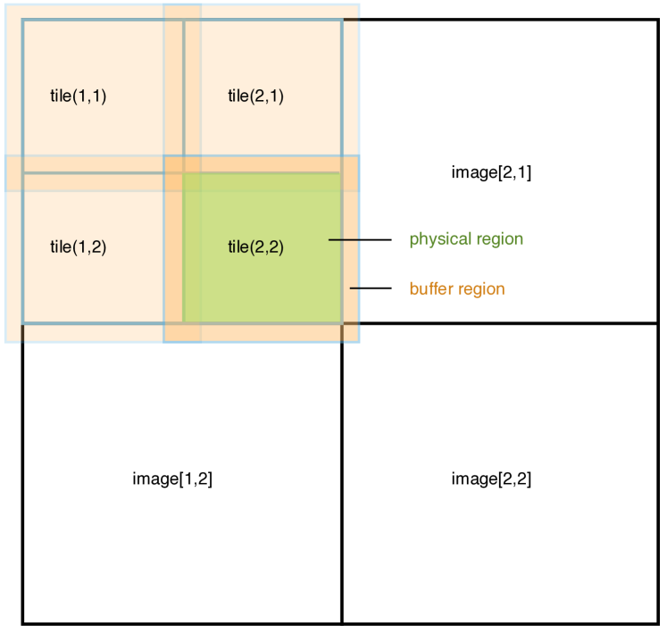
Figure 2.— Spatial decomposition in CUBE in a 2D analogy. In this example, there are two images per dimension ($M_{g}=2$), and two tiles per image per dimension ($M_{t}=2$). The orange boxes show the overlapped extended($V_{e}$)$\,=\,$physical($V_{p}$)$\,\cup\,$buffer($V_{b}$) tile regions. One physical region is indicated in green.

The simulation results are very insensitive if we manually tune the variance of the model $\sigma_{\Delta}$ within an order of magnitude. However, in the $n_{\nu}=1$ case, the method of using uneven bins gets much better results than simply using equal bins between minimum and maximum values $[\min(\Delta v),\max(\Delta v)]$. So, one can safely use a standard $\Lambda$CDM (cold dark matter with a cosmological constant as dark energy) for slightly different cosmological models, in equation (4). In CUBE, the velocity conversion takes the formula

$$\nu_{d}=\left\lfloor(2^{8n_{\nu}}-1)\pi^{-1}\tan^{-1}\left((v_{d}-v_{c})\sqrt{\pi/2\sigma_{\Delta}^{2}}\right)\right\rfloor,$$ (6)

$$v_{d}=v_{c}+\tan\left(\frac{\pi\nu_{d}}{2^{8n_{\nu}}-1}\right)\sqrt{2\sigma_{\Delta}^{2}/\pi},$$ (7)

where $\lfloor\ \rfloor$ is the operator to take the nearest integer. Tangent functions are convenient and computing-efficient. Compared to the error functions used in the Gaussian case, they take the same variance at $\nu_{d}=0$ but resolve high velocities relatively better. All possible choices of conversion formulae and $\sigma_{\Delta}$ are unbiased in the conversion Equations (6,7), however, a proper choices optimize the velocity space sampling and can result in more precise results.

Initially, particles are generated by an initial condition generator, at a higher redshift. The coarse grid velocity field $v_{c}$ is also generated at this step by averaging all particles in the coarse cell. A global $\sigma_{\Delta}$ is calculated by equation (5), where linear approximation holds. Then, velocities are stored by equation (6). During the simulation, $v_{c}$ is updated every time-step, and a nonlinear $\sigma_{\Delta}$ is measured directly from the simulation, and can be simply used in the next time step, after scaled by the ratio of growth factors between two adjacent time-steps. For more details see section 2.3.3.

2.3. Code overview

CUBE uses a 2-level PM force calculation. In order to apply the integer-based format to the $N$-body simulation, substantial structural changes need to be done. CUBE is written in Coarray Fortran, where Coarray features replace MPI (Message Passing Interface) communications between computation nodes/images. The algorithm is described in this language.

2.3.1 Spatial decomposition

CUBE decomposes the global simulation volume into $M_{g}^{3}$ cubic sub-volumes with $N_{c}$ coarse grids or $N_{f}=RN_{c}$ fine grids per side. The fine mesh is usually $R=4$ times finer than the coarse mesh. Each of these sub-volumes is assigned to a coarray image. Inside of an image, the sub-volume is further decomposed into $M_{t}^{3}$ cubic tiles (defined as $V_{p}$, or a physical region) with $N_{c}/(M_{g}M_{t})$ coarse grids per side. Each $V_{p}$ is surrounded by a buffer region $V_{b}$ which is $N_{b}$ coarse cells thick. We define the extended tile region as $V_{e}\equiv V_{p}\cup V_{b}$. $V_{e}$ is designed for two purposes:

(1) If the short fine mesh force ${\boldsymbol{F}}_{f}$ has a cut-off, $N_{b}$ ${\boldsymbol{F}}_{f}(r>N_{b})=0$, and is computed on $V_{e}$, then ${\boldsymbol{F}}_{f}$ in $V_{p}$ is guaranteed to be correct.

(2) $V_{e}$ is able to collect all particles that are able to travel to $V_{p}$.

Figure 2 shows the spatial decomposition in a 2-dimensional analogy, with $M_{g}=2$ and $M_{t}=2$.

According to this spatial decomposition, and as discussed in the last two subsections, we declare $\{\rho_{c},v_{c},\chi_{d},\nu_{d}\}$ by using Fortran language:

$${\color[rgb]{.5,0,.5}{\tt integer(1)}}\ \ \,\rho_{c}(N_{e},N_{e},N_{e},M_{t},M_{t},M_{t})[M_{g},M_{g},*]$$

$${\color[rgb]{.5,0,.5}{\tt real(4)}}\ \ \ \ \ \ \ \,v_{c}(N_{e},N_{e},N_{e},M_{t},M_{t},M_{t})[M_{g},M_{g},*]$$

$${\color[rgb]{.5,0,.5}{\tt integer(}n_{\chi}{\tt)}}\,\chi_{d}(3,P_{\rm max})[M_{g},M_{g},*]$$

$${\color[rgb]{.5,0,.5}{\tt integer(}n_{\nu}{\tt)}}\ \nu_{d}(3,P_{\rm max})[M_{g},M_{g},*]$$

where $N_{e}=N_{t}+2N_{b}$ covers the buffer region on both sides, $M_{t}$ is the tile dimensions, and $M_{g}$ is the image co-dimensions. We denote the actual number of particles in a given image as $P_{\rm local}$, and $P_{\rm max}>P_{\rm local}$ is a value (discussed in Section 2.4) large enough to store particles in $V_{e}$. $\chi_{d}$ and $\nu_{d}$ must be sorted according to the same memory layout as $\rho_{c}$, such that $n_{c}$ and $x_{d}$ can be obtained from equation (2). $\{\rho_{c},v_{c},\chi_{d},\nu_{d}\}$ provides a complete information on the positions and velocities of particles, and we call it a checkpoint.

An additional particle-ID (PID) array, $I_{P}$, can also be declared to differentiate particle types (e.g. CDM and neutrino particles) or to differentiate every particle, by using an $n_{I}$-byte integer per particle. If PID is turned on, the array $I_{P}$ is also included in the checkpoints, and the ordering of $I_{P}$ is the same as that for $\chi_{d}$ and $\nu_{d}$.

program Initial_Condition_Generator_for_CUBE
  calculate $\Phi$ in Fourier space
  do (each tile)
    do (each particle at ${\boldsymbol{q}}\in V_{e}$)
      ${\boldsymbol{\Psi}}({\boldsymbol{q}})=\nabla\Phi({\boldsymbol{q}})$
      $\{{\boldsymbol{q}},{\boldsymbol{\Psi}({\boldsymbol{q}})}\}\rightarrow\{{\boldsymbol{x}},{\boldsymbol{v}}\}$
      $\{{\boldsymbol{x}},{\boldsymbol{v}}\}\rightarrow\{\rho_{c},v_{c}\}$
     enddo
    do (each particle at ${\boldsymbol{q}}\in V_{e}$)
      ${\boldsymbol{\Psi}}({\boldsymbol{q}})=\nabla\Phi({\boldsymbol{q}})$
      $\{{\boldsymbol{q}},{\boldsymbol{\Psi}({\boldsymbol{q}})}\}\rightarrow\{{\boldsymbol{x}},{\boldsymbol{v}}\}$
      calculate particle’s index $i$ according to $\rho_{c}$
      ${\boldsymbol{x}}\rightarrow\chi_{d}(:,i);\,\{{\boldsymbol{v}},v_{c}\}\rightarrow\nu_{d}(:,i)$
      if (PID_flag) create $I_{P}(i)$
    enddo
    do (each coarse grid $\in V_{e}$)
      delete particles $\in V_{b}$
    enddo
    write $\{\rho_{c},v_{c},\chi_{d},\nu_{d}\}$ to disk
    sum up $P_{\rm local}$
  enddo
  sync all
  sum up $P_{\rm global}$
end

Figure 3.— Pseudocode for the initial condition generator.

2.3.2 Initial conditions

The cosmological initial condition generator is compiled and run separately from the main $N$-body code. Here, we briefly describe it for completeness.

The first step is the calculation of the displacement potential $\Phi$. At an initial redshift $z_{i}$, we generate a linear density fluctuation $\delta_{L}({\boldsymbol{q}})$ on Lagrangian grid ${\boldsymbol{q}}$ by multiplying a Gaussian random field with the transfer function $T(k)$ (given by the assumed cosmological model) in Fourier space. Then, we solve for the potential ${\Phi({\boldsymbol{q}},z_{i})}$ of a curlless displacement field ${\boldsymbol{\Psi}({\boldsymbol{q}})}$ by Poisson equation $-\nabla^{2}\Phi=\delta_{L}$ in Fourier space.

The second step to generate particles and displace them by Zel’dovich approximation (ZA) (Zel’dovich, 1970), where the displacement field is obtained by differentiating $\Phi$, is ${\boldsymbol{\Psi}}({\boldsymbol{q}})=\nabla\Phi({\boldsymbol{q}})$ in real space. This step is done on $V_{e}$ of each tile.

We iterate twice over particles’ ${\boldsymbol{q}}$ in $V_{e}$. The first iteration calculates particles’ ${\boldsymbol{x}}$ and ${\boldsymbol{v}}$ by ZA and obtains $\rho_{c}$ and $v_{c}$ on the coarse grid. The second iteration’s ${\boldsymbol{x}}$ and ${\boldsymbol{v}}$ are calculated again and are converted to $\chi_{d}$ and $\nu_{d}$ by Equations (1,6) and placed in a certain order according to $\rho_{c}$. Lastly, we delete particles in $V_{b}$, and re-sort the ones in $V_{p}$ and write $\{\rho_{c},v_{c},\chi_{d},\nu_{d},I_{P}({\rm optional})\}$ of this tile to disk. The above is similar to update_xp of Section 2.3.3. If PIDs are needed, they are also generated here. After working on all tiles, we sum up $P_{\rm local}$ and $P_{\rm global}$. We summarize the above steps into a pseudocode in Figure 3. During this step, the only major memory usage is $\Phi$ on the fine mesh. If the number of particles per fine grid $P_{f}=1$, the memory consumption of this in-place FFT is 4 bpp.

program CUBE
  call initialize
  call read_particles
  call buffer_density
  call buffer_xp
  call buffer_vp
  do
    call timestep
    call update_xp
    call buffer_density
    call buffer_xp
    call update_vp
    call buffer_vp
    if(checkpoint_step) then
      call update_xp
      call checkpoint
      if (final_step) exit
      call buffer_density
      call buffer_xp
      call buffer_vp
    endif
  enddo
  call finalize
end

Figure 4.— Overall structure of CUBE. Sections of the code are grouped into Fortran subroutines, which are described in paragraphs of Section 2.3.3.

2.3.3 Algorithm

Figure 4 shows the overall structure of the main code.

initialize creates fine mesh and coarse mesh FFT plans, and reads in configuration files telling the program at which redshifts we need to do checkpoints, halofinds, or stop the simulation. Force kernels $K_{c}$, $K_{f}$ are also computed or loaded.

read_particles, from the disk, reads in a checkpoint $\{\rho_{c},v_{c},\chi_{d},\nu_{d},I_{P}({\rm optional})\}$ for each image. Because they exist only in the $V_{p}$ of every tile, they are disjoint; and they provide complete information on the whole simulation volume – we call it “disjoint state”. In this state, $\rho_{c}$, $v_{c}$’s values in buffer regions, and $\chi_{d}(:,P_{\rm local}+1:)$ and $\nu_{d}(:,P_{\rm local}+1:)$ are 0’s. Because $I_{P}$ is generated and manipulated together with $\nu_{d}$, so we do not explicitly mention $I_{P}$ in the followings.

buffer_density, buffer_x and buffer_v convert the “disjoint” state to the “buffered state”. In buffer_density, $V_{b}$ regions of $\rho_{c}$ are synchronized between tiles and images. By buffer_x, $\chi_{d}$ is updated to contain common, buffered particles, and they are sorted according to the buffered $\rho_{c}$. buffer_v deals with $\nu_{d}$ in a similar manner.

timestep is a second order Runge-Kutta method is used in the time integration, i.e., for $n$ time-steps, we update positions ($D$=drift) and velocities ($K$=kick) at interlaced half time-steps by operator splitting; the operation $({\rm DKKD})^{n}$ is second-order accurate. The actual simulation applies varied time-steps by timestep, where a time increment ${\rm d}t$ is constrained by particles’ maximum velocities, accelerations, cosmic expansion, and any other desired conditions.

subroutine update_xp
  do (each physical tile)
    do (each particle)
      $\{\rho_{c},\chi_{d}\}\rightarrow{\boldsymbol{x}};\,\{v_{c},\nu_{d}\}\rightarrow{\boldsymbol{v}}$
      ${\boldsymbol{x}}={\boldsymbol{x}}+{\boldsymbol{v}}\,{\rm d}t$
      update $\rho_{c}^{*},\,v_{c}^{*}$ according to ${\boldsymbol{x}}$
    enddo
    do (each particle)
      $\{\rho_{c},\chi_{d}\}\rightarrow{\boldsymbol{x}};\,\{v_{c},\nu_{d}\}\rightarrow{\boldsymbol{v}}$
      ${\boldsymbol{x}}={\boldsymbol{x}}+{\boldsymbol{v}}\,{\rm d}t$
      calculate particle’s index $i$ according to $\rho_{c}^{*}$
      ${\boldsymbol{x}}\rightarrow\chi_{d}^{*}(:,i);\,\{{\boldsymbol{v}},v_{c}\}\rightarrow\nu_{d}^{*}(:,i)$
    enddo
    do (each coarse grid)
      discard buffer information
    enddo
    replace $\{\rho_{c},v_{c},\chi_{d},\nu_{d}\}$ with $\{\rho_{c}^{*},v_{c}^{*},\chi_{d}^{*},\nu_{d}^{*}\}$
  enddo
  sync all
  update velocity dispersion $\sigma^{2}_{\Delta}$
  sum up $P_{\rm local},\,P_{\rm global}$
end

Figure 5.— Pseudocode for subroutine update_xp.

update_xp is used, according to ${\rm d}t$, to update particle positions (drift $D$) in a “gather” algorithm tile by tile. For each particle, $\chi_{d}$ and $\nu_{d}$ are converted to $x_{d}$ and $v_{d}$ by Equations(2,7).

In order to keep particles ordered, for each tile, we first perform $x_{d}=x_{d}+v_{d}\,{\rm d}t$ on all particles to obtain an updated density and velocity field on the tile, $\rho_{c}^{*}$ and $v_{c}^{*}$. Then, this calculation is done on the same tile again to generate a new, local particle list $\chi_{d}^{*}$ and $\nu_{d}^{*}$ by Equations(1,6). Here, the ordering of $\chi_{d}^{*}$ and $\nu_{d}^{*}$ relies on $\rho_{c}^{*}$. Then, the third iteration is done on this tile to delete buffer regions of $\{\rho_{c}^{*},v_{c}^{*},\chi_{d}^{*},\nu_{d}^{*}\}$. Then the disjoint state of $\{\rho_{c}^{*},v_{c}^{*},\chi_{d}^{*},\nu_{d}^{*}\}$ replaces the old $\{\rho_{c},v_{c},\chi_{d},\nu_{d}\}$. Finally, $P_{\rm local}$ and $P_{\rm global}=\sum P_{\rm local}$ are updated. These steps are summarized in Figure 5.

In update_vp the PM or PP particle-mesh (P³M) algorithm is applied in this subroutine to update particles’ velocities (kick $K$). We first call buffer_density and buffer_xp to place the particle positions in the buffered state. Then, according to the particle distributions $\rho_{f}$ on $V_{e}$, we calculate the fine mesh force ${\boldsymbol{F}}_{f}$ and update the particle velocities in the $V_{p}$. An optional PP force ${\boldsymbol{F}}_{\rm pp}$ (subroutine PP_force) can be called to increase the force resolution.

subroutine update_vp
  do (each extended tile)
    call PP_force
    calculate $\rho_{f}$ and solve ${\boldsymbol{F}}_{f}$ in Fourier space
    do (each particle in physical region)
      $\nu_{d}\rightarrow{\boldsymbol{v}},\,{\boldsymbol{v}}={\boldsymbol{v}}+{\boldsymbol{F}}_{f}{\rm d}t,\,{\boldsymbol{v}}\rightarrow\nu_{d}$
    enddo
    update $\max(|{\dot{\boldsymbol{v}}}|)$
  enddo
  calculate $\rho_{c}$ and solve ${\boldsymbol{F}}_{c}$ in Fourier space
  do (each particle)
    $\nu_{d}\rightarrow{\boldsymbol{v}},\,{\boldsymbol{v}}={\boldsymbol{v}}+{\boldsymbol{F}}_{c}{\rm d}t,\,{\boldsymbol{v}}\rightarrow\nu_{d}$
  enddo
  update $\max(v_{d}),\max(|{\dot{\boldsymbol{v}}}|)$
end

Figure 6.— Pseudocode for subroutine update_vp.

The compensating coarse grid force ${\boldsymbol{F}}_{c}$ is globally computed by using a coarser- (usually by a factor of $R=4$) mesh by dimensional splitting – the cubic distributed coarse density field $\rho_{c}$ is transposed (inter-image) and Fourier transformed (inner-image) in three consecutive dimensions. After the multiplication of memory-distributed force kernel $K_{c}$, the inverse transform takes place to get the cubic distributed coarse force field ${\boldsymbol{F}}_{c}$, upon which velocities are updated again.

For each type of velocity update, the collective operations are Equation(7), ${\boldsymbol{v}}={\boldsymbol{v}}+{\boldsymbol{F}}_{\rm total}$, and Equation(6). We also update $\sigma^{2}_{\Delta}$ according to the new $v_{d}-v_{c}$. These steps are summarized in Figure 6.

After the updating of $\nu_{d}$ in $V_{p}$, we simply call buffer_v again to bring $\nu_{d}$ into the buffered state, such that the update_x in the next iteration will be done correctly.

For checkpoint, if a desired redshift is reached, we execute the last drift step in the $({\rm DKKD})^{n}$ operation by update_xp, and call checkpoint to save the disjoint state of $\{\rho_{c},v_{c},\chi_{d},\nu_{d}\}$ on the disk. Other operations like run-time halo-finder or density projections are also done at this point.

Finally, in the finalize subroutine we destroy all the FFT plans and finish up any timing or statistics taken in the simulation.

2.4. Memory layout

Here, we list the memory-consuming arrays and how they scale with different configurations of the simulation. We classify them into (1) arrays of particles, (2) coarse mesh arrays, and (3) fine mesh arrays.

2.4.1 Arrays of particles

These arrays comprise the majority of the memory usage, and contain checkpoint arrays $\chi_{d}$, $\nu_{d}$, $I_{P}$, and temporary arrays $\chi_{d}^{*}$, $\nu_{d}^{*}$, $I_{P}^{*}$. The former uses memory $\mathcal{M}=(3n_{\chi}+3n_{\nu}+n_{I})P_{\rm max}\,{\rm byte}$, where

$$P_{\rm max}=\left\langle P_{\rm local}\right\rangle\left(1+\frac{2N_{b}}{N_{t}}\right)^{3}(1+\epsilon_{\rm image}),$$ (8)

and $\left\langle P_{\rm local}\right\rangle$ is the average number of particles per image. The second term, proportional to $V_{e}/V_{p}$, lets us store additional particles in $V_{b}$, and the third term $1+\epsilon_{\rm image}$ takes into account the inhomogeneity of $P_{\rm local}$ on different images. When each image models smaller physical scales, $\epsilon_{\rm image}$ should be set larger.

Temporary $\chi_{d}^{*}$, $\nu_{d}^{*}$, $I_{P}^{*}$ store particles only on tiles, and the particle number is set to be

$$P_{\rm max}^{*}=\left\langle P_{\rm local}\right\rangle\left(\frac{1}{M_{t}}\right)^{3}(1+\epsilon_{\rm tile}),$$ (9)

where $\epsilon_{\rm tile}$ controls the inhomogeneity on scales of tiles. Larger $M_{t}$ causes more inhomogeneity on smaller tiles, and $\epsilon_{\rm tile}$ can be much larger than $\epsilon_{\rm image}$; however, the term $M_{t}^{-3}$ decreases much faster. Practically, the majority memory is occupied by $\chi_{d}$, $\nu_{d}$, $I_{P}$.

Summarizing the above, we find that the memory usage per particle (bpp) ${\mathcal{M}}_{P}\equiv{\mathcal{M}}/\left\langle P_{\rm local}\right\rangle/{\rm byte}$, given $n_{\chi}=n_{\nu}=1$ and $n_{I}=0$, is

$$\mathcal{M}_{P}^{\rm particle}=6\Big{[}(1+2N_{b}N_{t}^{-1})^{3}(1+\epsilon_{\rm image})$$

$$+M_{t}^{-3}(1+\epsilon_{\rm tile})\Big{]}.$$ (10)

Because $N_{t}=N_{c}/(M_{g}M_{t})$, we can minimize Equation (2.4.1) by tuning $M_{t}$.

2.4.2 Coarse mesh arrays

On coarse mesh, $\rho_{c}$ (4-byte integers), $v_{c}$, and force kernel $K_{c}$ should always be kept. They are usually configured to be $R=4$ times coarser than fine grids and particle number density. They have use memories of $(1+3)\times 4\times(N_{e}M_{t})^{3}+3\times 4\times(N_{c}/M_{g})^{3}/2$ bytes per image, or

$$\mathcal{M}_{P}^{\rm coarse}=P_{c}^{-1}\left[16\left(1+\frac{2N_{b}}{N_{t}}\right)^{3}+6\right],$$ (11)

where $P_{c}$ is the average number of particles per coarse cell. Other coarse-grid-based arrays are $\rho_{c}^{*}$, $F_{c}$, and pencil-FFT arrays. $\rho_{c}^{*}$ exists only on tiles; $F_{c}$ and pencil-FFT arrays can be equivalenced with other temporary arrays. Thus, the majority of the memory usage from coarse FFT arrays comes from Equation (11).

2.4.3 Fine mesh arrays

On the local fine mesh, only a force kernel array $K_{f}$ needs to be kept. It has memory of $3\times 4\times(RN_{e}M_{t})^{3}/2$ per image, or

$$\mathcal{M}_{P}^{\rm fine} = 6P_{f}^{-1}N_{t}^{-3}\left(1+\frac{2N_{b}}{N_{t}}\right)^{3}$$ (12)

$$= 6R^{3}P_{c}^{-1}N_{t}^{-3}\left(1+\frac{2N_{b}}{N_{t}}\right)^{3},$$

where $P_{f}$ is the average number of particles per fine cell. For the fine mesh density arrays, force field arrays are temporary. Since $\chi_{d}^{*}$, $\nu_{d}^{*}$, coarse force arrays, and pencil-FFT arrays are also temporary and are not used in any calculation simultaneously, they can be overlapped in memory by using equivalent statements.

Table 1Memory layout for a certain configuration

		Memory usage
Type	Array	/GB	/bpp	Percentage
Particles	$\chi_{d}$, $\nu_{d}$	29.9	8.24	83.8%
	$\chi_{d}^{*}$, $\nu_{d}^{*}$	3.16	0.872	8.87%
	$I_{P}$, $I_{P}^{*}$	0	0	0%
	Subtotal	33.0	9.12	92.7%
Coarse mesh	$\rho_{c}$	0.296	0.0818	0.831%
	$v_{c}$	0.889	0.245	2.49%
	$K_{c}$	0.340	0.0939	0.954%
	$F_{c}$	(0.690)	(0.190)	(1.94%)
	$\rho_{c}^{*}$	0.0140	0.00388	0.0394%
	Pencil-FFT	(0.454)	(0.125)	(1.27%)
	Subtotal	1.55	0.429	4.36%
Fine mesh	$K_{f}$	1.06	0.292	2.97%
	$F_{f}$	(1.63)	(0.450)	(4.57%)
	Fine-FFT	(1.41)	(0.389)	(3.96%)
	Subtotal	1.06	0.292	2.97 %
Total		35.6	9.84	100%
Optimal limit		21.7	6	61.0%

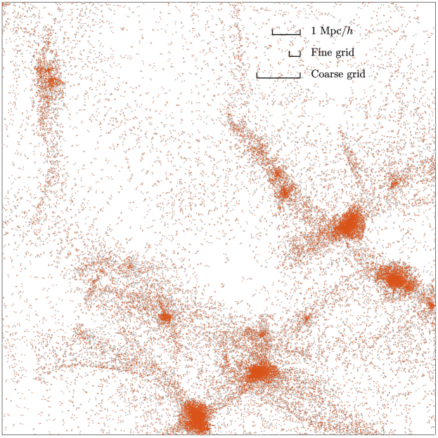
Figure 7.— Offset in the particle distribution induced by an integer-1 based algorithm (x1v1). In S512’s subregion of volume $15.625^{2}\times 3.90625\ ({\rm Mpc}/h)^{3}$, particles from CUBEP3M (the larger gray dots in the background) and CUBE-x1v1 (the smaller red dots) are projected onto the plane of $(15.625\ {\rm Mpc}/h)^{2}$. The comparing rules show 1 ${\rm Mpc}/h$, for fine and coarse grids respectively, and position resolution of x1v1 is 1/64 of a fine grid.

2.4.4 Compare with traditional algorithms

To illustrate the improvement of memory usage, we refer to the TianNu simulation (Yu et al., 2017b) run on the Tianhe-2 supercomputer, which used a traditional $N$-body code CUBEP3M. TianNu’s particle number (shown in Table 2) is limited by memory per computing node – for each computing node, an average of $576^{3}$ neutrino particles and $288^{3}$ CDM particles are used, and consumes $\mathcal{M}=40\,{\rm GB}$, or about $\mathcal{M}_{P}=186$. A memory-efficient configuration of CUBEP3M by using large physical scales and at costs of speed, still uses about $\mathcal{M}_{P}=40$.

If the same amount of memory is allocated to CUBE, we can set parameters as $n_{\chi}=n_{\nu}=1$, $N_{c}/M_{g}=384$, $N_{b}=6$, $\epsilon_{\rm image}=5\%$, $\epsilon_{\rm tile}=200\%$ and thus $\left\langle P_{\rm local}\right\rangle=1536^{3}$. Setting $M_{t}=3$ (27 tiles per image) minimizes $\mathcal{M}$ and uses about $\mathcal{M}=35.6\,{\rm GB}$, corresponding to $\mathcal{M}_{P}=9.84$. This can be done on most of the supercomputers, even modern laptops.

Table 1 shows the memory consumption for this test simulation. The memory-consuming arrays are listed and classified into the three types above mentioned, and their memory usages are in units of GB ($10^{9}$ byte), bpp, and their percentage of the total memory usage. The parenthesized numbers show overlapped memory, which is saved by equivalencing them with the underscored numbers. There are other unlisted variables that are memory-light, and can also be equivalenced with the listed variables.

In the bottom of Table 1 we stress that the optimal memory usage is 6 bpp, or 21.7 GB, 61% of the actual $\mathcal{M}$. The dominating departure from this limit is that $\chi_{d}$ and $\nu_{d}$ already occupy 8.24 bpp, which come from the $(1+2N_{b}/N_{t})^{3}$ term of Equation (2.4.1). All other variables occupy an additional 8%. On modern supercomputers, the memory per computing node is usually much larger, and by scaling up the number of particles per node, the buffer ratio $N_{b}/N_{t}$ will be lowered and we can approach closer to the 6 bpp limit.

Table 2Simulation configurations

	Configurations
Name	$N_{\rm node}$	$L/({\rm Mpc\,}h^{-1})$	$z_{i}$	$N_{p}$	$m_{p}/M_{\odot}$
S512	8	200	49	$512^{3}$	$7.5\times 10^{9}$
S256	1	80	49	$256^{3}$	$3.8\times 10^{9}$
S2048S	64	400	49	$2048^{3}$	$9.4\times 10^{8}$
S2048L	64	1200	49	$2048^{3}$	$2.5\times 10^{10}$
TianNu	13824	1200	100	$6912^{3}$	$6.9\times 10^{8}$
			5	$13824^{3}$	$3.2\times 10^{5}$
TianZero	13824	1200	100	$6912^{3}$	$7.0\times 10^{8}$

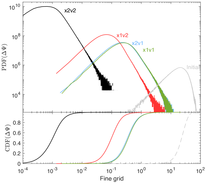
Figure 8.— Statistics of the error in particle displacement $\Delta{\boldsymbol{\Psi}}$ induced by integer-based algorithms in CUBE. The PDF and CDF of $|\Delta{\boldsymbol{\Psi}}|$ from S256 are shown in the upper and lower axes, as functions of fine grids. Black, red, blue, and green correspond to x2v2, x1v2, x2v1, and x1v1, respectively. The gray lines, marked with “initial”, show the distribution of the actual displacement of particles in CUBEP3M, $|{\boldsymbol{\Psi}}_{0}|$, which is orders of magnitudes larger than $|\Delta{\boldsymbol{\Psi}}|$.

3. Accuracy

We run a group of simulations to test the accuracy of CUBE. We use the same seeds to generate the same Gaussian random fields in the initial condition generators of CUBEP3M and CUBE, and then they produce initial conditions of their own formats. Then, the main $N$-body codes run their own initial conditions to redshift $z=0$. We use the same force kernels as CUBEP3M without PP force. Note that near the find grid scales, it is possible to enhance the force kernel to better match the nonlinear power spectrum predictions; however, we use the conservative mode of CUBEP3M in this paper. An extended PP force and an unbiased force matching algorithm will be added to CUBE. The power spectrum studies are presented in Harnois-Déraps et al. (2013), while here we focus on the cross-correlations between different integer-based methods.

First, by using different configurations – different numbers of computing nodes, box sizes, particle resolutions, different number of tiles per node/image, etc., we find that by using 2-byte integers for both positions and velocities ($n_{\chi}=n_{\nu}=2$, or x2v2) allows CUBE to give exact results compared to CUBEP3M. So if sufficient memory is provided, one can always use x2v2 to get exact results as CUBEP3M, and the optimal memory limit of this case is 12 bpp, which is still much lower than traditional methods. Next, we focus on the accuracy of the other three cases – x1v2, x2v1, and x1v1.

We list the names and configurations of the simulations used in Table 2, where $N_{\rm node}$, $L$, $z_{i}$, $N_{p}$, and $m_{p}$ are respectively the number of computing nodes used, the length of the side of the box, initial redshift, total number of particles, and particle mass. These configurations are run by CUBEP3M, x2v2, x1v2, x2v1, and x1v1 versions of CUBE with the same initial seeds. Using different numbers of tiles per image gives the exact same results. We also list the configurations for TianNu and TianZero (Yu et al., 2017b; Emberson et al., 2017) simulations as a reference.

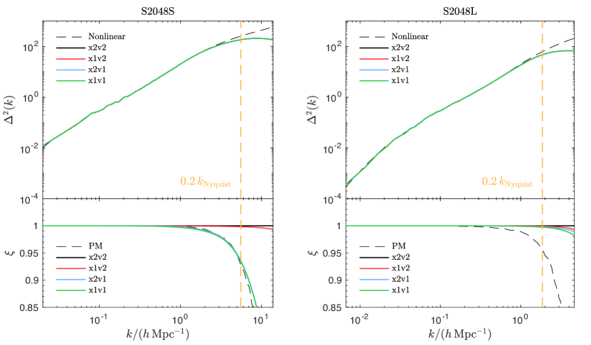
Figure 9.— Dimensionless power spectra $\Delta^{2}(k)$ and the cross-correlations $\xi(k)$ (lower axes) with respect to x2v2 in simulations S2048S and S2048L. The four solid lines show the results from {x2v2,x1v2,x2v1,x1v1}. In the lower panels, the dashed curves show the decorrelations given by the PM algorithm, measured by cross-correlating different resolutions of CUBE-x2v2. The vertical orange dashed lines show the scale $k=0.2\,k_{\rm Nyquist}$.

3.1. Power spectrum

3.2. Displacement of particles

In S512, we zoom-in on a small region of $15.625^{2}\times 3.90625\ ({\rm Mpc}/h)^{3}$ and compare the particle distribution between CUBEP3M and CUBE-x1v1 in Figure 7. For clarity, CUBEP3M particles are marked with the larger gray dots, whereas the smaller red dots are CUBE-x1v1 particles overplotted onto them. The 1 ${\rm Mpc}/h$, fine grid, and coarse grid scales are shown in the figure. The position resolution of particles in CUBE-x1v1 is 1/256 of a coarse grid, or 1/64 of a fine grid.

To quantify the offset in the final particle distributions, we use PIDs to track the displacement ${\boldsymbol{\Psi}}({\boldsymbol{q}})\equiv{\boldsymbol{x}}-{\boldsymbol{q}}$ of every particle (Yu et al., 2017a), where ${\boldsymbol{x}}$ and ${\boldsymbol{q}}$ are Eulerian and Lagrangian coordinates of the particle. Then, we calculate the absolute value of the offset vector

$$\Delta\Psi\equiv|{\boldsymbol{\Psi}}_{i}-{\boldsymbol{\Psi}}_{0}|.$$ (13)

Here, ${\boldsymbol{\Psi}}_{0}$ stands for CUBEP3M and subscript _i can stand for x2v2, x1v2, x2v1, or x1v1. The PDFs and CDFs of $\Delta\boldsymbol{\Psi}$ in S256 are shown in Figure 8. Results from x2v2, x1v2, x2v1, or x1v1 are in black, red, blue, and green respectively. The results from absolute displacement of particles (by replacing ${\boldsymbol{\Psi}}_{i}$ with ${\boldsymbol{q}}$ in Equation (13)) are shown in gray for comparison.

For x2v2, almost all particles are accurate up to 1/100 of a fine grid, and the worst particle is $\sim 1/10$ of a fine grid away from its counterpart in CUBEP3M. The difference is caused by round-off errors and is negligible in physical and cosmological applications. The accuracy of x1v2 is between x2v2 and x1v1, and x2v1 gives only a minor improvement from x1v1. We also run a simulation with the same number of particles but with $L=600\ {\rm Mpc}/h$ ($m_{p}=1.2\times 10^{12}M_{\odot}$), and find that the accuracy of x1v2 is in turns between x2v1 and x1v1. We interpret that, in this latter case, particles have lower mass resolution, so they move slower and need higher position resolution but need lower velocity resolution, thus x2v1 outperforms x1v2.

S2048S and S2048L are two simulations with $2048^{3}$ particles in small ($L=400\ {\rm Mpc}/h$) and large ($L=1200\ {\rm Mpc}/h$) box sizes. We compare their accuracy by their power spectra and their cross-correlations with CUBEP3M at $z=0$. The physical scale of S2048S is designed such that the particle mass resolution $m_{p}$ is comparable to TianNu and TianZero simulations (their parameters are also listed in Table 2). On the other hand, S2048L focuses on larger structures, on which scale one can study weak gravitational lensing, BAO (Eisenstein et al., 2005), and its reconstruction (Eisenstein et al., 2007; Wang et al., 2017), etc.

For each simulation the particles are firstly cloud-in-cell (CIC) interpolated onto the fine mesh grid, and from the density field $\rho$ we define the density contrast $\delta\equiv\rho/\left\langle\rho\right\rangle-1$. We define the cross-power spectrum $P_{\alpha\beta}(k)$ between two fields $\delta_{\alpha}$ and $\delta_{\beta}$ ($\delta_{\alpha}=\delta_{\beta}$ for auto-power spectrum) in Fourier space as

$$\left\langle\delta_{\alpha}^{\dagger}({\boldsymbol{k}})\delta_{\beta}({\boldsymbol{k}}^{\prime})\right\rangle=(2\pi)^{3}P_{\alpha\beta}(k){\boldsymbol{\delta}}_{\rm 3D}({\boldsymbol{k}}-{\boldsymbol{k}}^{\prime}),$$ (14)

where ${\boldsymbol{\delta}}_{\rm 3D}$ is the 3D Dirac delta function. In cosmology we usually consider the dimensionless power spectrum $\Delta^{2}_{\alpha\beta}(k)\equiv k^{3}P_{\alpha\beta}(k)/(2\pi^{2})$. The cross-correlation coefficient is defined as

$$\xi(k)\equiv P_{\alpha\beta}/\sqrt{P_{\alpha\alpha}P_{\beta\beta}}.$$ (15)

In the upper two panels of figure 9 we show the power spectra of CUBE. In both plots of S2048S and S2048L the four solid curves of different colors show the results of x2v2, x1v2, x2v1, and x1v1, and they almost overlapped with each other. The dashed curves are the nonlinear prediction of the matter power spectrum by CLASS (Blas et al., 2011).

We label $k=0.2\,k_{\rm Nyquist}$ as vertical dashed lines, where $k_{\rm Nyquist}$ is the scale of fine mesh grids, and the scale of average particle separations. On this scale, the power spectra are offset from nonlinear predictions by at least 20%. This error is from the PM algorithm and one has to increase the resolution of the simulation to correct these offsets. We do not plot CUBEP3M because we found that CUBEP3M and x2v2 of CUBE produce same results. Thus, the differences between CUBEP3M and different integer formats of CUBE are negligible compared to the error of the PM algorithm.

In the lower parts of these four panels we study the cross-correlations. We compare everything with CUBE-x2v2, to emphasize the decorrelation (i.e. $1-\xi(k)$) by different integer formats. Note that x2v2 is perfectly correlated with CUBEP3M. In the lower two panels of figure 9 the solid curves show the decorrelation $\xi$ of x1v2, x2v1, and x1v1. The higher resolution (S2048S) in general comes with more decorrelations, and x1v2 cross-correlates with x2v2 better than the other two cases. In order to quantify the PM error in terms of decorrelations, we run x2v2 simulations with the same initial conditions, but 8 times more particles and cells, and measure the decorrelation caused by coarser resolutions. These results are shown as dashed curves (labeled “PM”). We conclude that the cross-correlation of x1v1, in all cases, is not worse than the PM errors.

To summarize from Figure 9, in terms of either power spectrum deviation or cross-correlation, the error induced by information optimization (even for x1v1) is lower than the error from the PM algorithm, and we can safely use x1v1 for most of the LSS studies.

4. Discussion and conclusion

We present a parallel, information-optimized $N$-body algorithm. This open-source code, CUBE, has recently been used in many studies of LSS, e.g. Yu et al. (2017a); Wang et al. (2017); Pan et al. (2017). It requires very low memory usage, approaching 6 bpp.

The accuracy of this code is adjustable in that we can choose 1-byte/2-byte integers separately for positions and velocities of particles. In the case of using 2 byte integers for both positions and velocities (“x2v2”, and memory can be 12 bpp), the algorithm gives the exact results given by traditional $N$-body algorithms. Note that the results are exactly the same in that they not only produce the same physical statistics of LSS, but also the same error (not physical) from the PM algorithm near Nyquist frequencies. In other words, the positions and velocities of each particle are exact. In practice, we only require that the errors from information optimization is much lower than the errors from the PM algorithm. In Figure 9 we see that this is the case even for the most memory-efficient configuration, x1v1. This shows that in most LSS studies, when our scales of interest are smaller than $k\simeq 0.2\,k_{\rm Nyquist}$, six 1-byte fixed point numbers contain sufficient information of every $N$-body particle.

Another benefit of this algorithm is LSS simulations with neutrinos, although the neutrino modules of CUBE are in development. Neutrinos have a high velocity dispersion and move much faster than CDM, and their small-scale errors are dominated by their Poisson noise. We expect that, compared to CDM, x1v1 gives less power spectrum deviation to neutrinos, as they behave more Gaussian and are less clustered. LSS-neutrino simulations, like TianNu, can contain much more (for TianNu, 8 times more) neutrino $N$-body particles than CDM, which dominate the memory. For a TianNu-like simulation, one can safely use x1v2 or x2v2 for CDM and x1v1 for neutrinos, and the memory usage can approach 6 bpp. This allows much more particles to be included in the simulation and can lower the Poisson noise of neutrinos prominently. A 1-byte PID per particle increases minor memory usage and can differentiate eight kinds of particles, or we can store different particles in different arrays without using PID.

We did not include PP force in CUBE and CUBEP3M in this paper. If one wants to focus on smaller scales, like halo masses and profiles, an extended PP forces, which act up to adjacent fine cells, should be taken into account. The memory consumption for PP force is only local and is negligible compared to particles. In these cases where even x2v2 is used, a 12 bpp memory usage is still much lower than that of traditional $N$-body algorithms.

Traditional $N$-body codes consume considerable memory while performing relatively light computations. CUBE is designed to optimize the efficiency of information and the memory usage in $N$-body simulations. CUBE is written in Coarray Fortran – concise Coarray features are used instead of complicated MPI – and the code itself is much more concise than CUBEP3M for future maintenance and development. The next steps are optimization of the code and adapting it for various kinds of heterogeneous computing systems, e.g. MIC and GPUs. Optimizing the velocity storage may further improve the accuracy of x1v1, and whose effects on neutrino-LSS simulation are yet to be discovered.

References

- Angulo et al. (2012) Angulo, R. E., Springel, V., White, S. D. M., et al. 2012, MNRAS, 426, 2046
- Appel (1985) Appel, A. W. 1985, SIAM Journal on Scientific and Statistical Computing, vol. 6, no. 1, January 1985, p. 85-103., 6, 85
- Blas et al. (2011) Blas, D., Lesgourgues, J., & Tram, T. 2011, J. Cosmology Astropart. Phys., 7, 034
- Couchman (1991) Couchman, H. M. P. 1991, ApJ, 368, L23
- Couchman et al. (1995) Couchman, H. M. P., Thomas, P. A., & Pearce, F. R. 1995, ApJ, 452, 797
- Davis et al. (1985) Davis, M., Efstathiou, G., Frenk, C. S., & White, S. D. M. 1985, ApJ, 292, 371
- Dehnen (2014) Dehnen, W. 2014, Computational Astrophysics and Cosmology, 1, 1
- Dubinski et al. (2004) Dubinski, J., Kim, J., Park, C., & Humble, R. 2004, New A, 9, 111
- Eisenstein et al. (2007) Eisenstein, D. J., Seo, H.-J., Sirko, E., & Spergel, D. N. 2007, ApJ, 664, 675
- Eisenstein et al. (2005) Eisenstein, D. J., Zehavi, I., Hogg, D. W., et al. 2005, ApJ, 633, 560
- Emberson et al. (2017) Emberson, J. D., Yu, H.-R., Inman, D., et al. 2017, Research in Astronomy and Astrophysics, 17, 085
- Frigo & Johnson (2005) Frigo, M., & Johnson, S. G. 2005, in PROCEEDINGS OF THE IEEE, 216–231
- Harnois-Déraps et al. (2013) Harnois-Déraps, J., Pen, U.-L., Iliev, I. T., et al. 2013, MNRAS, 436, 540
- Hilbert et al. (2009) Hilbert, S., Hartlap, J., White, S. D. M., & Schneider, P. 2009, A&A, 499, 31
- Hockney & Eastwood (1988) Hockney, R. W., & Eastwood, J. W. 1988, Computer simulation using particles
- Merz et al. (2005) Merz, H., Pen, U.-L., & Trac, H. 2005, New A, 10, 393
- Pan et al. (2017) Pan, Q., Pen, U.-L., Inman, D., & Yu, H.-R. 2017, MNRAS, 469, 1968
- Pen (1995) Pen, U.-L. 1995, ApJS, 100, 269
- Potter & Stadel (2016) Potter, D., & Stadel, J. 2016, PKDGRAV3: Parallel gravity code, Astrophysics Source Code Library, , , ascl:1609.016
- Rimes & Hamilton (2005) Rimes, C. D., & Hamilton, A. J. S. 2005, MNRAS, 360, L82
- Rokhlin (1985) Rokhlin, V. 1985, Journal of Computational Physics, 60, 187
- Sato et al. (2009) Sato, M., Hamana, T., Takahashi, R., et al. 2009, ApJ, 701, 945
- Springel (2005) Springel, V. 2005, MNRAS, 364, 1105
- Springel et al. (2001) Springel, V., Yoshida, N., & White, S. D. M. 2001, New A, 6, 79
- Springel et al. (2005) Springel, V., White, S. D. M., Jenkins, A., et al. 2005, Nature, 435, 629
- Takahashi et al. (2009) Takahashi, R., Yoshida, N., Takada, M., et al. 2009, ApJ, 700, 479
- Takahashi et al. (2011) —. 2011, ApJ, 726, 7
- Teyssier (2010) Teyssier, R. 2010, RAMSES: A new N-body and hydrodynamical code, Astrophysics Source Code Library, , , ascl:1011.007
- Vale & White (2003) Vale, C., & White, M. 2003, ApJ, 592, 699
- Wang et al. (2017) Wang, X., Yu, H.-R., Zhu, H.-M., et al. 2017, ApJ, 841, L29
- Xu (1995) Xu, G. 1995, ApJS, 98, 355
- Yu et al. (2018) Yu, H.-R., Pen, U.-L., & Wang, X. 2018, CUBE: Information-optimized parallel cosmological N-body simulation code, Astrophysics Source Code Library, , , ascl:1805.018
- Yu et al. (2017a) Yu, H.-R., Pen, U.-L., & Zhu, H.-M. 2017a, Phys. Rev. D, 95, 043501
- Yu et al. (2017b) Yu, H.-R., Emberson, J. D., Inman, D., et al. 2017b, Nature Astronomy, 1, 0143
- Zel’dovich (1970) Zel’dovich, Y. B. 1970, A&A, 5, 84