The effect of neutrinos on the matter distribution as probed by the Intergalactic Medium
Abstract:
We present a suite of full hydrodynamical cosmological simulations that quantitatively address the impact of neutrinos on the (mildly non-linear) spatial distribution of matter and in particular on the neutral hydrogen distribution in the Intergalactic Medium (IGM), which is responsible for the intervening Lyman- absorption in quasar spectra. The free-streaming of neutrinos results in a (non-linear) scale-dependent suppression of power spectrum of the total matter distribution at scales probed by Lyman- forest data which is larger than the linear theory prediction by about 25 % and strongly redshift dependent. By extracting a set of realistic mock quasar spectra, we quantify the effect of neutrinos on the flux probability distribution function and flux power spectrum. The differences in the matter power spectra translate into a () difference in the flux power spectrum for neutrino masses with eV (0.6 eV). This rather small effect is difficult to detect from present Lyman- forest data and nearly perfectly degenerate with the overall amplitude of the matter power spectrum as characterised by . If the results of the numerical simulations are normalized to have the same in the initial conditions, then neutrinos produce a smaller suppression in the flux power of about 3% (5%) for eV (1.2 eV) when compared to a simulation without neutrinos. We present constraints on neutrino masses using the Sloan Digital Sky Survey flux power spectrum alone and find an upper limit of eV (2 C.L.), comparable to constraints obtained from the cosmic microwave background data or other large scale structure probes.
1 Introduction
One of the most exciting results in particle physics in the last decade has been that neutrinos have been established to be massive particles. Solar, atmospheric, reactor and accelerator neutrino experiments have confirmed the existence of flavour oscillations of active neutrinos, implying that neutrinos have non-zero mass (see Ref. [1] and references therein). This is generally considered as definite evidence for new physics beyond the Standard Model. The neutrino oscillation experiments do, however, not pin down the absolute neutrino masses. The experiments instead provide a lower limit for the sum of the neutrino masses of eV. Current measurement of the matter power spectrum from Cosmic Microwave Background (CMB) data extrapolated to smaller scales alone already give an upper limit on the sum of the neutrino masses of about eV well below what has been reached with particle physics experiments leaving an allowed range of only a factor about twenty for the sum of the neutrino masses. There is thus very strong motivation to push hard for an actual measurement of neutrino masses. The tritium -decay experiment KATRIN111http://www-ik.fzk.de/katrin is the most ambitious current direct detection experiment and is expected to probe an electron neutrino mass of eV in the near future (see [2] for a recent review).
The matter distribution in the Universe is sensitive to the free-streaming of cosmological neutrinos. Astrophysical constraints are therefore a very competitive alternative method to measure/constrain the masses of neutrinos. Measurements of the matter power spectrum can in principle probe neutrino masses significantly smaller than the upper limit from CMB experiments. Early on the neutrinos are relativistic and travel at the speed of light with a free-streaming length equal to the Hubble radius. Neutrinos in the mass range eV eV, become non-relativistic in the redshift range . In the mass range of degenerate neutrino masses the thermal velocities can be approximated as,
| (1) |
As a result present-day velocities (of the most massive neutrino species) range between 100 km/s for the upper and and 3000 km/s for the lower end of the still allowed range of the sum of the neutrinos masses. Dark matter particles with such a high velocity dispersion are usually called hot dark matter. A dominant contribution of hot dark matter to the total dark matter content would be at odds with current observations. Neutrinos in the still allowed mass range instead constitute a sub-dominant contribution complementing cold dark matter comprised of some other elementary particle, such as neutralinos or axions.
The effect of cosmological neutrinos on the evolution of density perturbation in the linear regime is well understood. Neutrinos affect both the cosmic expansion rate and the growth of structure ([3, 1]). The neutrino contribution in terms of energy density can be expressed as:
| (2) |
where is the present value of the Hubble constant in units of 100 km/s/Mpc and is the matter energy density in terms of the critical density.
When neutrinos become non relativistic in the matter dominated era, there is a minimum wavenumber
| (3) |
above which the physical effect produced by neutrino free-streaming damps small-scale neutrino density fluctuations, while modes with evolve according to linear theory. The free-streaming leads to a suppression of power on small scales which in linear theory can be approximated by for . With increasing energy content in neutrinos (corresponding to increasing neutrino mass) the suppression becomes larger and its shape and amplitude depends mainly on and weakly on redshift [4]. At scales Mpc the suppression is constant while at scales it gradually decreases to zero. At very large scales the effect of neutrinos on the matter power spectrum becomes negligible. These different scales are roughly those that are currently probed by Lyman- forest data, galaxy surveys, and CMB experiments, respectively.
A large number of studies have used the effect of neutrinos on the matter power spectrum (or perhaps better the lack thereof) to put upper limits on the energy content and therefore the masses of neutrinos. Unfortunately, there is no single data set yet which fully covers the characteristic imprint of neutrinos on the matter power spectrum and the reliability of these limits therefore depends strongly on the somewhat questionable assumption that there are no systematic offsets between measurements of the matter power spectrum with different methods which are not reflected in the quoted measurement errors.
The Lyman- forest data thereby plays a special role in probing the effect of the free-streaming of neutrinos on the matter power spectrum as it allows us to measure the matter power spectrum on the scales where the suppression due to neutrinos is most pronounced while still being in the mildly non-linear regime ([5, 6], see Ref. [7] for a more general review of the IGM). Ref. [8] have used high resolution spectra to obtain an early still rather weak limit of eV from Lyman- forest data alone. Ref. [9] have claimed a rather extreme limit of eV (2 C.L.) based on the Sloan Digital Sky Survey (SDSS) quasar data set, combined with other large scale structure probes. This is the tightest limit obtained so far from cosmological data. Other measurements using cosmic microwave background data, galaxy redshift surveys and growth of clusters of galaxies are usually a factor three to six larger than this (e.g. [10, 11, 12, 13, 14, 15]). Note, however, also the rather low upper limit of eV (2 C.L.) obtained by [16] based on Luminous Red Galaxies (LRG) in the SDSS Data Release 7 combined with data on the scale of Baryonic Acoustic Oscillations and the luminosity distance of distant supernovae. Forecasts for future CMB, weak lensing and Lyman- forest data obtained by Planck 222http://sci.esa.int/science-e/www/area/index.cfm?fareaid=17, the Baryon Oscillation Spectroscopic Survey 333http://www.sdss3.org/cosmology.php and other surveys are presented e.g. in [17, 1, 18, 19].
We would like, however, to stress again that the validity of current limits depends strongly on the assumption that there are no systematic offsets between estimates of the matter power spectrum obtained with different methods which are not reflected in the quoted measurement errors. To make further progress it will be very important to identify the characteristic signatures of the effect of neutrinos on the detailed shape of the matter power spectrum and its evolution with redshift. The Lyman- forest data has here again particular potential as it covers on its own a reasonably wide redshift range. With the Lyman- forest Baryonic Acoustic Oscillations (BAO) survey planned as part of the Sloan Digital Sky Survey (SDSS-3) it should be possible to reach the scales where the suppression due to neutrinos becomes scale dependent.
While linear theory is sufficient to quantify the impact of neutrinos on large scales and on the cosmic microwave background, the non-linear evolution of density fluctuations has to be taken into account on smaller scales at lower redshift. A range of numerical studies of the effect of neutrinos on the distribution of (dark) matter has been performed some while ago (e.g.[4, 20, 21]) with a renewed interest in the last couple of years ([22, 23, 24]). These numerical studies of the non-linear evolution have been complemented by analytical estimates based on the renormalization group time-flow approach [25, 26], perturbation theory [27, 28] or the halo model [29, 30].
The use of Lyman- forest data for accurate measurements of the matter power spectrum benefits tremendously from the careful modeling of quasar absorption spectra with hydrodynamical simulations (e.g. [31]). No such modeling has yet been performed including the effect of neutrinos. We will be closing this gap here and present results of the modeling of Lyman- forest data in the non-linear regime including the effect of neutrinos by using a modified version of the hydrodynamical code GADGET-3.
Modeling the effect of neutrinos in the mass range of interest is non-trivial due to their rather large thermal velocities. We mainly focus here on an implementation of the neutrinos as a separate set of particles. Ref. [23] have recently suggested to model the neutrinos with a grid based approach as a neutrino fluid instead of neutrino particles. In this approach the gravitational force due to neutrinos is calculated based on the linearly evolved density distribution of the neutrinos in Fourier space. This approach has the advantage that it does not suffer from the significant shot noise on small scales introduced by the particle representation of the fast moving neutrinos yielding higher accuracy at scales and redshifts where the effect of the non-linear evolution of the neutrinos is still moderate especially for small neutrino masses.
In addition to our particle based neutrino simulations we have also experimented with such a grid based implementation of neutrinos. In this implementation the linear growth of the perturbation in the neutrino component is followed by interfacing the hydrodynamical code with the public available Boltzmann code CAMB444http://camb.info/.
Further advantages of such a grid based implementation of neutrinos, aside from eliminating the Poisson noise, are the reduced requirements with regard to memory (there are no neutrino positions and velocities to be stored) and computational time. However, as we will demonstrate in Section 3 for the scales and redshift of interest for the Lyman- forest data, non-linear effects are important. Taking their effect into account with the particle-based implementation actually offers a somewhat higher accuracy despite the reduction of the shot noise at the smallest scales offered by a grid based implementation of the linear evolution of the neutrino density.
The main improvement of our work presented here compared to previous studies are the use of full hydrodynamical simulations in a regime in which baryons are expected to significantly impact on the matter power (e.g. [32]), the focus on small scales and high redshift and the estimate of statistical properties of the Lyman- flux distribution.
The outline of the paper is as follows. In Section 2 we describe the numerical methods and how we generate the initial conditions for the different simulations. Section 3 quantifies the impact of the neutrino component on the matter power spectrum. In this section we also address the role of numerical parameters such as the initial redshift, number of neutrino particles, Poisson noise and velocities in the initial conditions. Section 4 focuses on the impact of neutrinos on two statistics of the flux distribution in Lyman- forest spectra, the flux probability distribution function and the flux power spectrum. Section 5 presents the upper limit on the sum of the neutrino masses that we have obtained from the SDSS flux power spectrum alone. Section 6 summarizes our conclusions.
We recall that the scales of interest for the Lyman- forest low-resolution SDSS spectra are Mpc, or s/km. High-resolution spectra as the UVES/Large Programme LUQAS sample reach Mpc [33]. The results for neutrinos and matter power spectra will be presented as a function of wavenumber in units of Mpc, while those that refer to (one-dimensional) flux power spectrum will be cast in terms of s/km. The conversion between wavenumbers expressed in s/km and Mpc is redshift dependent and is given by the factor which for the cosmology used below is 99, 111.5 and 123.6 km/s/Mpc, at redshifts , , and , respectively.
2 The simulations
| linear size (Mpc) | N | N | PM1/3 | (eV) | |||
| 60 | 0.3 | 512 | 512 | – | 0.15 | 0.325 | 7 |
| 60 | 0.3 | 512 | 512 | – | 0.3 | 0.65 | 7 |
| 60 | 0.3 | 512 | 512 | – | 0.6 | 1.3 | 7 |
| 60 | 0.3 | 512 | 512 | – | 1.2 | 2.6 | 7 |
| 60 | 0.3 | 512 | 1024 | – | 0.6 | 1.3 | 7 |
| 60 | 0.3 | 512 | 1024 | – | 0.15 | 0.325 | 7 |
| 60 | 0.3 | 512 | – | – | – | – | 7 |
| 60 | 0.3 | 512 | – | – | – | – | 4 |
| 60 | 0.3 | 512 | – | – | – | – | 49 |
| 60 | 0.3 | 384 | – | – | – | – | 7 |
| 60 | 0.3 | 512 | 512 | – | 0.15 | 1.3 | 4 |
| 60 | 0.3 | 512 | 512 | – | 0.15 | 1.3 | 49 |
| 60 | 0.2 | 512 | 512 | – | 0.6 | 1.3 | 7 |
| 60 | 0.4 | 512 | 512 | – | 0.6 | 1.3 | 7 |
| 60 | 0.6 | 512 | 512 | – | 0.6 | 1.3 | 7 |
| 512 | 0.3 | 512 | – | – | – | – | 7 |
| 512 | 0.3 | 512 | – | – | – | – | 49 |
| 512 | 0.3 | 512 | 512 | – | 0.6 | 1.3 | 7 |
| 512 | 0.3 | 512 | 512 | – | 0.6 | 1.3 | 49 |
| 60 | 0.3 | 512 | – | 512 | 0.6 | 1.3 | 49 |
| 60 | 0.3 | 512 | – | 512 | 0.6 | 1.3 | 7 |
| 60 | 0.3 | 512 | – | 512 | 0.15 | 0.325 | 7 |
| 60 | 0.3 | 512 | – | 1024 | 0.6 | 1.3 | 49 |
| 512 | 0.3 | 512 | – | 512 | 0.6 | 1.3 | 49 |
In order to facilitate a straightforward comparison with the findings of [22], we have used the following cosmological model based on cold dark matter and a cosmological constant (CDM): , , , and ( km/s). For all our simulations, we use the hydrodynamical TreePM-SPH (Tree Particle Mesh-Smoothed Particle Hydrodynamics) code GADGET-3, which is an improved and extended version of the code described in Ref. [34]. We have modified the code in order to simulate the evolution of the neutrino density distribution. The neutrinos are treated as a separate collisionless fluid, just like the dark matter. In order to save computational time, most of our simulations assume however that the clustering of neutrinos on small scales is negligible and the short-range gravitational tree force in GADGET’s TreePM scheme is not computed for the neutrino particles. This means that the spatial resolution for the neutrino component is only of order the grid resolution used for the PM force calculation, while it is about an order of magnitude better for the dark matter, star and gas particles calculated with the Tree algorithm. We also implemented memory savings such that the number of neutrino particles can be made (significantly) larger than the number of dark matter particles, which helps to reduce the Poisson noise present in the sampling of the (hot) neutrino fluid.
In the grid based implementation the power spectra of the neutrino density component is interpolated in a table produced via CAMB of one hundred redshifts in total spanning logarithmically the range . The gravitational potential is calculated at the mesh points and the neutrino contribution is added when forces are calculated by differentiating this potential. We have checked that we have reached convergence with this number of power spectrum estimates and also explicitly checked that increasing the linear size of the PM grid by a factor two has an impact below the 1% level on the total matter power for the wavenumbers Mpc. For the grid simulations the starting redshift has been chosen as , well in the linear regime.
The initial conditions were generated based on linear matter power spectra separately computed for each component (dark matter, gas and neutrinos) with CAMB [35]. The total matter power spectrum was normalized such that its amplitude (expressed in terms of ) matched the prediction by CAMB at the same redshift. After some testing the starting redshift for most of our runs was chosen as a rather low to reduce the shot noise due to the neutrino particles. When generating the initial conditions, we picked random phases for the modes in -space but eliminated the Rayleigh sampling of the mode amplitudes in order to more accurately match the mean power expected in each mode, especially on large scales. This (artificially) reduces cosmic variance on the scale of the box, but since we are mainly interested in comparing power spectra at two different redshifts (i.e. in the relative growth), we do expect this effect to have a negligible impact on our main results. Initial neutrino velocities are drawn randomly from a Fermi-Dirac distribution (Eq. [1]). We have also tested a momentum pairing scheme in the initial conditions, as originally suggested in [21, 20], by splitting each neutrino particle into two particles, giving them half the original mass and equal but opposite thermal velocities. However, we found this to have no influence on our results.
We have used the Zeld́ovich approximation [36] to generate initial conditions. We acknowledge that the use of a second-order Lagrangian perturbation theory scheme as proposed by [37] and used in [22] should improve the accuracy for simulations with low starting redshifts. As we are mainly interested here in the relative effect due to the free-streaming of neutrinos and not an absolute measurement of the overall amplitude of the matter power spectrum at a given redshift this should, however, not be a concern.
We employ a simplified criterion for star formation to avoid spending most of our computational time on the small-scale dynamics of compact galaxies that form in our simulations. All gas particles whose overdensity with respect to the mean is above 1000 and whose temperature is less than are turned into star particles immediately. We have shown previously that such a star formation recipe has very little impact on Lyman- flux statistics [6, 38], but speeds up the simulations considerably. As in our previous simulations [6] the heating rates have been multiplied by a factor to achieve temperatures of the IGM at mean density at which are in better agreement with observational data. For the =0.6 eV case, the mass per simulation particle at our default resolution is , and for gas, dark matter and neutrinos, respectively.
In Table 1 we summarize the most important parameters of the main hydrodynamical simulations that we use in this study. We stress that the scales and redshifts probed by most of these simulations are very different from those explored in Refs. [22, 23, 24] but we have also run a few simulation with the same large box size to facilitate a comparison. Most of the simulations run for this work are moderately time consuming. For example, the fν=0.13 neutrino simulation took about 12 hours on 200 CPUs to reach , while increasing the number of neutrino particles by a factor eight for the same setup required 10 hrs on 512 CPUs, meaning that it has become about two times slower in terms of total computational expense. For comparison, the simulation of the fν=0.13 model with the same amplitude of the matter power spectrum took 12 hrs on 160 CPUs, so including neutrino particles slows down the code only by (all the above numbers refer to runs performed on the HPCS system DARWIN at Cambridge University). However, the memory requirements for storing a large number of neutrino particles are quite demanding, and are in fact the limiting factor for simulations with the particle based implementation of the neutrino density. Note that the grid based simulation of the small box size simulations has taken about 1.6 times less CPU time to run than the corresponding particle based simulation. The total CPU consumption for simulations with the smallest neutrino mass =0.15 eV is thereby about 10% larger than that for the largest mass we investigated =0.6 eV.
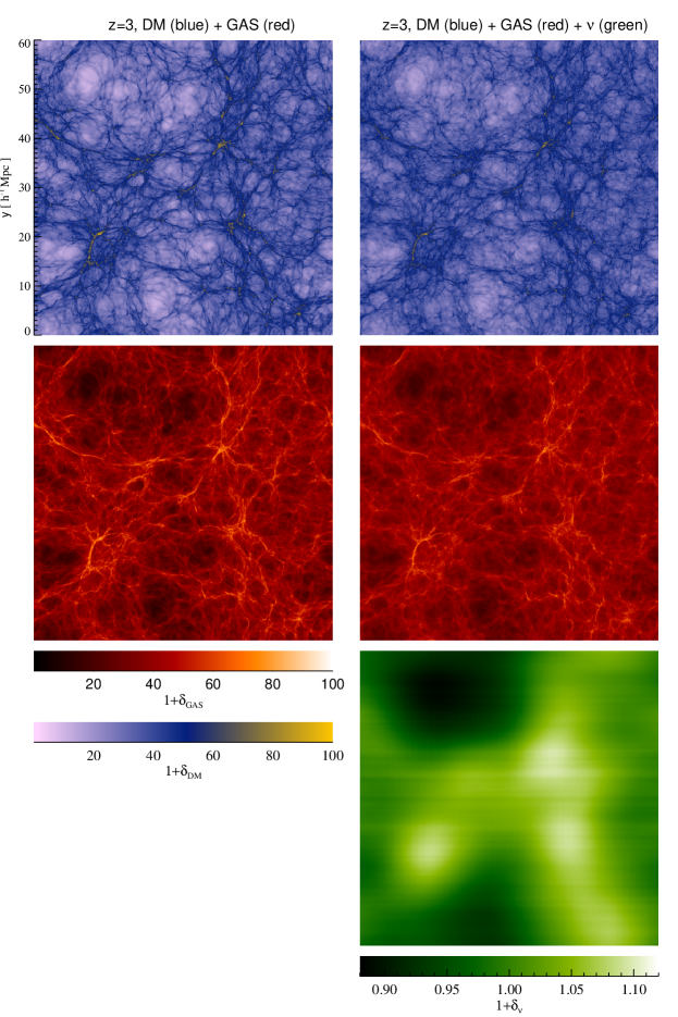
In Figure 1 we show illustrative slices of the density distribution of thickness 6 comoving Mpc extracted from two 60 comoving Mpc simulations at with and without neutrinos (for the particle based method). The left column shows a simulation with dark matter and gas but without neutrinos, while the right column shows the corresponding slices for the dark matter, gas and neutrinos for a three-component simulation with the same initial phases and =1.2 eV. The distribution of the neutrino density (in green, bottom panel) has been smoothed to eliminate spurious Poisson noise at the smallest scales in order to highlight that the genuine cosmological density fluctuations of the neutrinos occur only on large scales due to the free-streaming of the neutrinos. The growth of structure is clearly less evolved in the simulation with neutrinos (the voids are for example less empty), since the suppressed clustering of the neutrinos slows down the growth of the perturbations in the overall matter density. Typical neutrino fluctuations at the largest scales are about 10% around the mean, while fluctuations of the gas and dark matter density are usually much larger than this.
3 The matter power spectrum
3.1 Particle based vs. grid based implementation of neutrinos
In a series of papers Refs. [22, 23, 24] have recently discussed the relative benefits and drawbacks of implementing the effect of neutrinos in the form of particles taking into account the non-linear evolution of the gravitationally coupled neutrino, dark matter and gas components of the matter density and a grid based implementation accounting only for the effect of the linearly evolved neutrino density distribution. Here, we will primarily focus on modeling Lyman- forest data and are therefore interested in different scales and redshifts than those probed by other authors. However, in order to compare our work with that of Ref. [23] we performed some simulations with our grid and particle based implementation of neutrinos with a large box size of Mpc. These should correspond to simulations C1 and C3 of Ref. [23].
We measure the total matter power spectrum from the simulations by performing a CIC (Cloud-In-Cell) assignment to a grid of the same size as the PM grid used to compute the long-range gravitational forces. The smoothing effect of the CIC kernel is deconvolved when the density field at the grid points is obtained. Power spectra are computed for each component separately (gas, dark matter, stars and neutrinos), as well as for the total matter distribution.
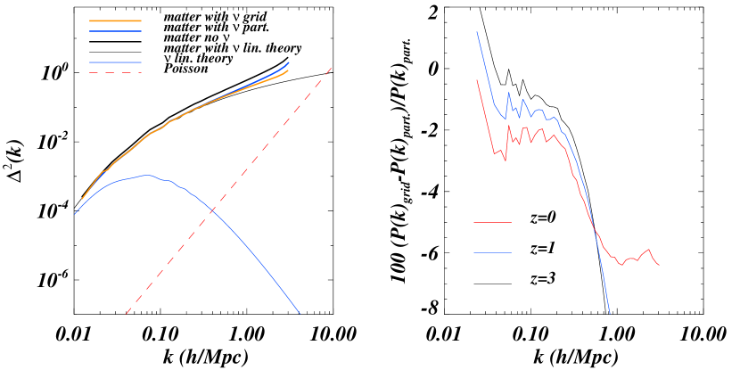
In the left panel of Figure 2 we compare the matter power spectra at in dimensionless units for simulations with neutrino mass =0.6 eV for the grid based (thick orange curve) and particle based (thick blue line) implementations with that of a simulation without neutrinos (thick black curve) and the prediction of linear theory (thin black curve). We also show the neutrino power spectrum (thin blue curves) and the (redshift independent) Poisson contribution (red dashed curve). The Poisson contribution (for the case) exceeds the neutrino power at Mpc. Only results for simulations with the large box size are shown. In the right panel we show the fractional difference of the matter power spectrum of simulations with the particle and grid based implementation of neutrinos at different redshifts (in percent). At large scales Mpc the differences are largest at , of the order of 2 % while at are smaller and around 1%. The results can be directly compared to those obtained by [23] for the same = 0.6 eV (figure 1 in their paper) but note that despite our attempt to choose similar parameters there may be still small differences in some of the parameters and that the simulations in [23] do not contain baryons. The discrepancies between the two implementations albeit small on large scales appear to be somewhat larger in our simulations.
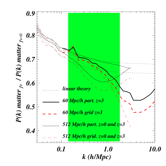
In Figure 3 we compare results from the two methods in terms of neutrino suppression for the large simulation box with results for a box size nearly ten times smaller ( Mpc), more appropriate for the modeling of Lyman- forest data. Large boxes are shown as thin curves which are red dashed in the grid implementation and black continuous in the particle one, respectively. Smaller boxes are reported as thick curves only at . At the smaller scales, that are not fully resolved by the large box-size simulation, non-linear effects are already important at the redshifts probed by Lyman- forest data and this is clearly demonstrated by the discrepancies between large and small scales. In fact, at (see left panel of Figure 2) and this non-linear evolution is missed in the large box simulations. We have checked that we get numerical convergence in terms of non-linear matter power spectra between the and the cases, so our results can be trusted at a quantitative level. We interpret this discrepancy as due to the fact that in simulations with the grid-based implementation the enforced linear evolution of the neutrinos with the same phases prevents a proper response to the dark matter growth. At the small scales Fourier mode mixing is important for the phase association and can alter the linear theory picture significantly. This appears to result in a significantly larger discrepancy between simulations with the grid and particle based implementations on the scales and redshifts relevant for Lyman- forest data. The differences between should thereby be mainly due to the fact that the non-linear evolution at small scales is not properly reproduced by the grid method. We will therefore focus mainly on simulations with the particle based implementation in the rest of the paper, keeping in mind that our results are affected by Poisson noise in the neutrino components at the smallest scales probed.
Note that increasing the accuracy of the simulations with the particle based neutrino implementation further by pushing up the number of neutrino particles in order to decrease the Poisson contribution to the matter power spectrum is rather demanding in terms of parallel computing resources. Increasing our default number of neutrino particles () by a factor of eight is still doable on the machine we had available for this (DARWIN) and requires a factor more CPU time. Increasing the default number of neutrino particles by a factor of 27 instead resulted, however, in prohibitive memory requirements. Further improvements in the accuracy of the simulations for future more accurate data sets will thus probably require optimization of the necessary compromises in a hybrid of the grid and particle based implementations as proposed by [24].
3.2 The effect of the neutrinos on the matter power spectrum
In this Section we first contrast the effect of the free-streaming of neutrinos on the power spectrum of the total matter density for a range of neutrino masses in full numerical simulation with that predicted by linear theory. We will only refer to results from simulations with the particle based implementations of neutrinos here, unless explicitly stated. In order to quantify the suppression of structure growth induced by neutrinos, we divide the matter power spectra of the neutrino simulations by the corresponding matter power spectrum extracted from the CDM simulation without neutrinos.

In Figure 4, we compare the non-linear power spectra from the numerical simulations with the results predicted by linear theory, shown as thick curves. The suppression of the matter power spectrum increases with increasing (recall that these simulations are normalized at the CMB scale). Note the plateau of constant suppression predicted by linear theory, which is approximately described by , and depends only very weakly on redshift. Linear theory provides a good description of the matter power spectrum at up to scales of about Mpc, and the agreement is more accurate for the smaller neutrino masses. The non-linear matter power spectrum does, on the other hand, depend strongly on redshift and the dependence on scale becomes steeper with decreasing redshift. For =0.6 eV, a good fit to the suppression at in the range that deviates from linear theory, , is given by at , respectively; while for =0.3 eV, we find at the same redshifts. We also note that the maximum reduction of power shifts to larger scales with decreasing redshift.
The maximum of the non-linear suppression can be described by (green thick curves in Fig. 4) for neutrino masses =0.15, 0.3, 0.6 eV, respectively. For the most massive case we considered the suppression is about . Our results differ somewhat from those of Ref. [22], who reported (at ) while we measure , apart from the most massive case in which the suppression is smaller, . We must remind, however, that the above linear approximation starts to break down for large neutrino masses and is already very poor for =1 eV (e.g. [1]).


Note that there is an up-turn in the suppression at scales of about , , /Mpc for , , , respectively. A similar upturn was found by Ref. [22], but at a scale of Mpc at . We have checked that this feature does not depend on the number of neutrino particles in the simulation. It does depend weakly on the value of (or ), moving to larger scales when is decreased. The upturn appears to be related to the non-linear collapse of haloes, which decouple from the large scale modes slightly differently in simulations with neutrinos than in simulations that have a different value for the amplitude of the power spectrum and no neutrinos. This suggests that the virialization of halos is slightly modified by the smoothly distributed neutrino component, in a similar fashion as done by dark energy where this is a well-known effect (see [39] for a recent study).
The main effect of the free-streaming of neutrinos is a reduction of the amplitude of the matter power spectrum on small scales. This results in a well known degeneracy between the values of and . In order to explore this degeneracy in more detail we have run four further hydrodynamical simulations without neutrinos that have the same value of at as the four different neutrino simulations, namely: = 0.137, 0.132, 0.122, and 0.103, mimicking the simulations with , , , and eV (note that the simulation without neutrinos has at ). The corresponding values are , , , , and for the default simulation. The differences in terms of the amplitude of density fluctuations range from 3% (0.15 eV) and 36% (1.2 eV). For the 0.6 eV simulations the difference is 15% which is very close to the corresponding uncertainty in the linear matter power spectrum amplitude at at scales s/km, as derived from SDSS Lyman- observations by [40].
The results of the simulations without neutrinos but a decreased power spectrum amplitude are shown in Figures 5 and 6, where we can see that the effects of neutrinos and a overall suppression of the matter power spectrum amplitude are very similar. For =0.15, eV the differences are at the percent level, while for the simulations with more massive neutrinos they differences increase to about 5-10%. In the rightmost panel of Fig. 6 ( =1.2 eV) , where the suppression is largest, we show the results of the neutrino simulations of Figure 4 for all three redshifts. On the small scales considered here the effect of the neutrinos on the non-linear matter power spectrum is to a high degree degenerate with an overall reduction of the matter power spectrum amplitude. The scale and redshift dependent differences to a simulation with an overall decrease of the power spectrum amplitude are small but nevertheless noticeable and increase with increasing neutrino mass. For neutrino masses with eV, the simulations with neutrinos typically show an additional suppression at the 5-10% level when compared to simulations without neutrinos with the same at . Note that Figure 6 is meant to highlight the small differences in the shape of the matter power spectra due to neutrinos if a normalization of the matter power spectrum at small scales is assumed (same , i.e. the fluctuations are effectively normalized at the Lyman- forest scale).
3.3 The effect of varying the total matter content
In the last section we had investigated the effect of varying the neutrino mass at fixed total matter content . In linear theory the effect of neutrinos is well parameterized by the ratio of mass content in neutrinos to total matter content, . We test here how well this holds for full non-linear simulations including neutrinos by varying at fixed neutrino mass. We have run simulations with and without neutrinos with and =0.6 eV. The results are shown in Figure 7. To further test the degeneracy with simulations with adapted value of we also run two simulations without neutrinos but with the same value as the simulations with . We overplot the results as thick curves. Note that this will mimic results obtained with simulations without neutrinos particles where the effect of neutrinos has been approximated by changing the (initial) power spectrum of the other matter components. This approximate approach has been taken by most studies in the past.

We note the same trends as before. The presence of neutrinos results in an additional suppression of the matter power that, is well parameterized by the quantity also in the non-linear regime. At fixed neutrino mass the suppression is therefore larger for smaller values of . For example, for it is twice larger than for and of about the same level of that we found for the fixed case. We thus conclude that the dependence of the matter power spectrum in the non-linear regime on the quantity is also well captured by the parameter . This is also demonstrated by the green line in the right-most panel of Figure 7 where the non-linear power spectra for the are overplotted on the result obtained for : the agreement is almost perfect at the scales of interest here, showing that also in the non-linear regime the parameter is the relevant quantity to describe the effect of neutrinos. We therefore conclude that on scales relevant for the Lyman- forest data the parameter is sufficient to characterize the effect of and the neutrino mass also on the non-linear power spectrum. although these results should be confirmed by using larger box size simulations, where possibly one starts to be more sensitive to the overall shape of the matter power spectrum.
3.4 Resolution tests and dependence on the initial conditions
In this subsection we investigate several numerical effects that impact the power spectra measurements presented in the previous section: the number of neutrino particles, the velocities in the initial conditions, the sampling of the initial conditions with neutrino pairs to balance momentum, and the starting redshift. Here we are not discussing resolution effects with regard to the number and mass of dark matter and gas particles since these have already been discussed extensively elsewhere with respect to the scales probed by Lyman- data (e.g. [6, 40, 41]). Furthermore, our results are mainly presented in terms of ratios of power spectra extracted from simulations with the same resolution. This strongly reduces the sensitivity to the dark matter and gas resolution.

First, we will take a closer look at the power spectrum of the neutrino component of the matter density. In Figure 8, we compare the non-linear neutrino power spectrum with predictions from linear theory for some of the simulations in Table 1. At scales of about Mpc the power spectrum starts to deviate strongly from linear theory and follows instead the expectation for Poisson noise, . The Poisson contribution to the power spectrum depends as expected on the number of neutrino particles used. This is demonstrated in the first and third panels where we also show results for simulations with =0.15, eV and instead of neutrino particles. Doubling the number of neutrino particles for each spatial dimension shifts the Poisson contribution to the matter power spectrum by a factor of roughly two to smaller scales.
When modeling the Lyman- forest flux power spectrum one ideally would like to sample the neutrino power spectrum properly on scales between 0.1 and 2 Mpc. As evident from Figure 8 this will be difficult as the neutrino distribution is affected by shot noise at the smallest relevant scales. Reducing this shot noise to negligible levels requires a number of neutrino particles with memory requirements beyond our current capabilities. In the following, we will see that despite the fact that the neutrino power spectrum is affected by shot noise at the smallest scales relevant for Lyman- studies, the impact on the one-dimensional flux power is still very small.
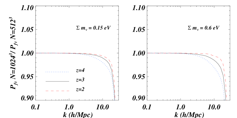
In Figure 9, we show the ratios of the (total) matter power spectra for a simulation with neutrino particles to that of our default simulations with neutrino particles, for = 0.15 eV (left panel) and = 0.6 eV (right panel). The increased number of neutrino particles results in an additional suppression of about 5-10% at scales above Mpc, while at the scales probed by the Lyman- forest the effect on the total matter power is of the order of 1% or less. While the Poisson contribution to the neutrino power spectrum is significant, its effect on the the total matter power spectrum is still small at small scales. The suppression is thereby slightly larger for = 0.6 eV, where the neutrinos constitute a larger fraction of the overall matter density. However, we should stress here that the Lyman- data is primarily sensitive the one-dimensional matter distribution along the line-of-sight (although cross-correlating information in the transverse direction is a promising tool for future observational data sets). The one-dimensional power spectrum, being a projection of the three-dimensional information, will be affected out to larger scales than the three-dimensional power spectrum by the suppression (or increase) of power at a given scale [42, 43].
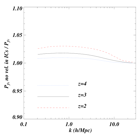
Next we will investigate the impact of the neutrino velocities assigned in the initial conditions. In Figure 10 we show for our default simulations with , the ratio of the matter power spectrum for a simulation without the thermal velocities relative to the matter power spectrum of a simulation where the velocities have been included in the initial conditions. Without the velocities in the initial conditions the power is less suppressed at Mpc by roughly 3%, 2% and 1% at , , and , respectively, with a very weak dependence on the wavenumber considered. These values are in good agreement with the results reported by Ref. [22].
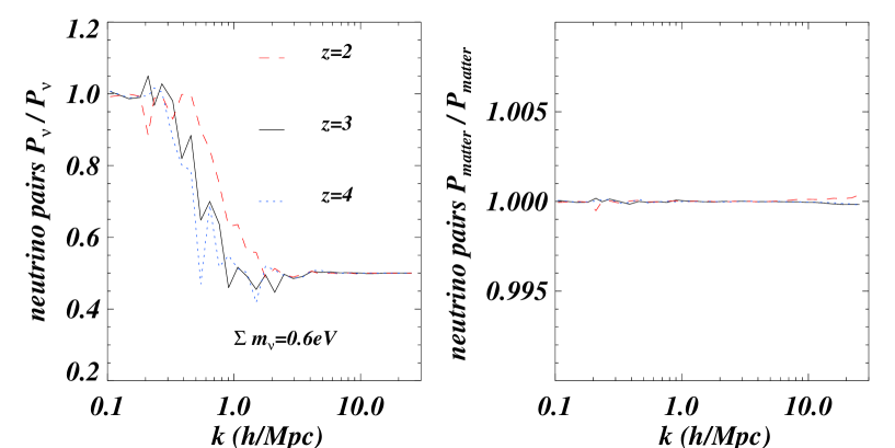
Another effect that could potentially affect our results are the details of the sampling of the initial phase-space density distribution of the neutrinos. Ref. [21] suggested that it would be advantageous to conserve momentum by creating pairs of neutrinos with equal and opposite thermal velocities. To test this, we modified the initial condition code to produce neutrino pairs with mass , instead of a single neutrino particle with mass . The two neutrino particles are then assigned the same velocities in opposite directions in order to conserve momentum. The results are shown in Figure 11, where we report the ratios of neutrino power spectra in the left panel and that of the matter power spectra in the right panel. The impact is very small and is fully accounted for by the different number of neutrino particles used, which decreases the Poisson contribution in the case of neutrino pairs by a factor of two at Mpc.
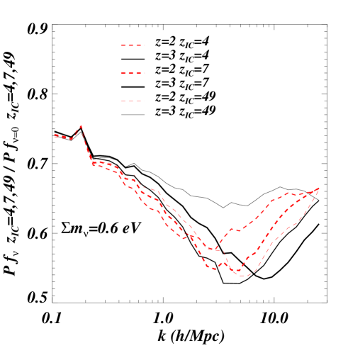
The last effect that we examine here is the dependence of the matter power spectrum on the initial redshift of the simulation [44, 45]. For this purpose we have performed four additional simulations with initial redshifts and for the simulation with = 0.6 eV and the CDM simulation without neutrinos. In Figure 12, we plot the suppression due to the effect of neutrinos for the matter power spectrum at and (black and red curves) for the three different values of the starting redshift. At Mpc there are differences of the order of 10% (3%) at (). As expected the results for our default simulation lie between those for the low and the high starting redshift. For the early starting redshift () the neutrino component becomes effectively Poissonian even at the largest scales, since the neutrino power spectrum as computed by CAMB will be in general much smaller at high redshift than the Poisson contribution (which is independent of redshift): this translates into a larger overall suppression of the matter power spectrum at small scales. Note that the different amount of Poisson power with respect to physical neutrino clustering in the initial conditions has an impact also on the subsequent clustering of the neutrino and matter components. For the low starting redshift (), the relevant scales are already affected by mildly non-linear growth. Note further that the relatively strong dependence on the initial redshift at is much more pronounced than that inferred by Refs. [22, 23], who found an overall agreement at the percent level at between simulations with different initial redshifts. This can probably be attributed at least partially to their use of second-order Lagrangian corrections in the initial conditions, which reduces the errors introduced when a low starting redshift is used. In addition, these authors studied much larger scales and by the non-linear evolution tends to largely erase the memory of differences in the initial conditions on small scales. For the purposes of our study appears to be an acceptable compromise. We provide further support for this in the next sections where we quantify the impact of the starting redshift on the Lyman- flux power spectrum.
4 The effect of neutrinos on statistics of the flux distribution in the Lyman- forest
4.1 Flux power and flux probability distribution function
In this Section we focus on the effect of neutrinos on the matter distribution as probed by the IGM, and in particular on the transmitted Lyman- flux and its one-point flux probability distribution function (PDF), and its two-point statistics (the flux power spectrum). To perform our analysis we have extracted 1000 mock quasar absorption spectra from the simulations at many different redshifts. All spectra are constructed in redshift space, taking into account the effect of the peculiar velocities of the IGM along the line-of-sight. The flux at redshift-space coordinate (in km/s/Mpc) can be written as with
| (4) |
where cm2 is the hydrogen Lyman- cross-section, is the Hubble constant at redshift , is the real-space coordinate (in km s-1), is the velocity dispersion in units of , is a Gaussian profile that approximates the Voigt profile well in the regime considered here.
The neutral hydrogen density in real-space in the equation above is approximately related to the underlying gas density (e.g. [46]) as,
where is the hydrogen photoionization rate in units of , is the IGM temperature, is the mean IGM density as a function of redshift and is the real-space coordinate.
As we have the benefit of a full hydrodynamical simulations there is, however, no need to make the approximations underlying equation (4.1). We calculate the integral in eq. (4) to obtain the Lyman- optical depth along each simulated line-of-sight using directly the relevant hydrodynamical quantities from the numerical simulations: . Further details on how to extract a mock quasar spectrum from an hydrodynamical simulation using the SPH formalism can be found in [47]. We have added noise typical for observed spectra and convolved the spectra with the instrumental resolution corresponding to observed high-resolution spectra. Note that the resolution has a larger effect on the flux PDF than the flux power spectrum. The ensemble of all our spectra have then been normalized by adjusting the assumed Ultra Violet background such that the observed mean flux level in high-resolution quasar spectra [48] at a given redshift, with is reproduced.
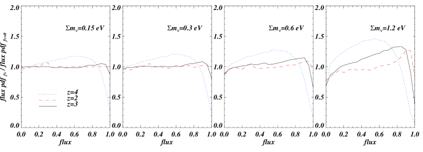
The Lyman- flux PDF is very well measured especially from high resolution quasar spectra (the statistical errors are at the percent level). We recently performed a careful analysis of the systematic uncertainties and were able to extract interesting astrophysical and cosmological constraints from the flux PDF [38]. In Figure 13, we show the ratio between the flux probability distribution functions of simulations with and without neutrinos: from left to right, the cases for , , , and eV are reported at , , and . The larger the neutrino masses , the more peaked the flux distribution becomes at intermediate flux values. The reason for this trend is that the growth of structure is suppressed in the simulation with neutrinos. As a result, voids (flux) are less empty and clustered regions are less dense than in the simulation without neutrinos and the effect is stronger at high redshift than at low redshift.
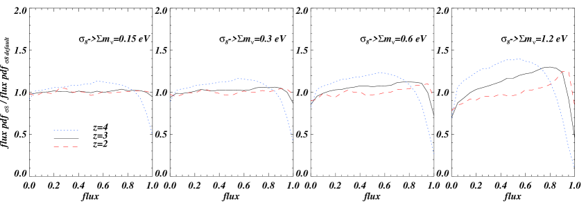
Analogous to our discussion in the previous section we also compute the flux properties for simulations without neutrinos but with a reduced overall amplitude of the matter power spectrum normalized to the same at . The results are shown in Figure 14. The trends with neutrino mass are similar to those seen in Figure 13, but slightly less pronounced.
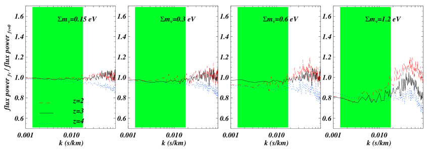
We now turn to the flux power spectrum, a quantity which is more closely related to the underlying matter power and has been extensively used to constrain cosmological and astrophysical parameters (e.g. [5]). The Lyman- flux power spectrum provides a more direct link to the matter power spectrum than the flux PDF: it is sensitive to cosmological parameters, the thermal state of the IGM, instrumental effects (signal to noise and resolution), the presence of metal lines and the nature of dark matter at small scales, etc. (see for example [33, 40]). The flux power spectrum has been measured over a wide redshift range, , using both high and low-resolution data. The growth of cosmic structures can thus be constrained over a significant fraction of the cosmic time, lifting the degeneracies between astrophysical and cosmological parameters that present different redshift and scale dependencies in this range.
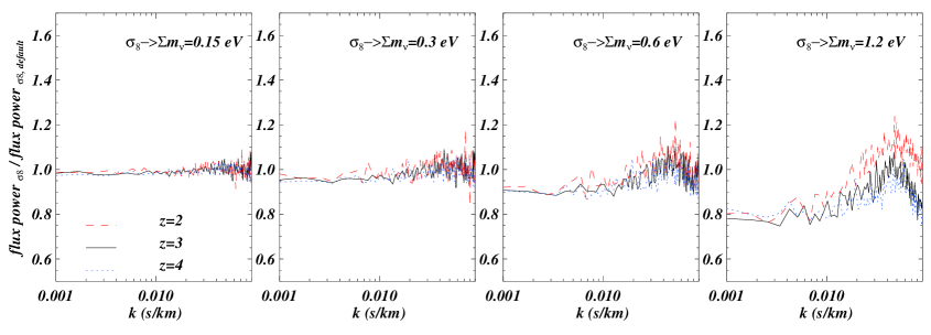
We show the measured flux power spectra for our different simulations in Figures 15 and 16. Note that the results have not been smoothed. We recall that the useful range of high resolution spectra reaches to s/km while we can reach to 0.018 s/km with low-resolution SDSS spectra. We are here primarily interested in quantifying the effects over this range of wavenumbers.
For =0.15 eV, the only effect of neutrinos on the flux power is a suppression at . As expected the effect becomes larger with increasing neutrino mass. At the largest scales the flux power in the simulations with neutrinos is suppressed by 5, 7 and 15% for = 0.3, 0.6 and 1.2 eV, respectively. There is some dependence of the suppression on wavenumber with an upturn at small scales of about 0.01 s/km and a bump at s/km.
The relationship between one-dimensional flux power spectrum and three-dimensional matter power is non-trivial, not only because of the fact that the one-dimensional matter power is an integral of the three-dimensional spectrum, but also due to non-linearities in the flux-density relation. As clearly demonstrated in Ref. [49], systems with column densities cm-2 contribute most to the flux power at s/km, and these absorbers are produced by gas which is close to the mean density [50]. The differences in the flux power spectrum of simulations with and without neutrinos reflect the differences in the spatial distribution of gas in models which have experienced different amounts of growth of structure: at , a model with a reduced amplitude of the matter power spectrum has more structure at mean density than a high- model for which the gas probability distribution function is more skewed. Note that the suppressions for the simulations without neutrinos in Figure 16 are very similar to those with a reduced amplitude of the matter power spectrum with the same value of . The small differences visible in the three dimensional matter power spectra are thus even smaller in the flux power spectrum.
4.2 Numerical effects on the flux power spectrum for simulations with the particle based implementation of neutrinos
In this subsection we explore the sensitivity of our results for the flux power spectrum on a number of numerical effects. In Figure 17, we show the ratios of the flux power spectrum for simulations with =0.15 eV (left panel) and =0.6 eV (right panel) with and neutrino particles. There is an opposite trend here to what we found in the corresponding plot for the matter power shown in Figure 9. There is a bump at s/km where the ratio rises above unity. The ratio of the matter power spectrum at a similar scale of Mpc does not change or is mildly suppressed. At these scales the matter power spectrum is affected by Poisson noise due to the neutrinos. The larger Poisson contribution to the matter power spectrum in the simulation with the smaller number of neutrinos should result in less diffuse small scale absorbers and lower the amplitude of the flux power spectrum at scales s/km.
We have also checked the effect of a different number of mesh points on the PM grid by running a simulation with and a PM grid of mesh points. We find that the impact is negligible in the range of scales of interest, about () at scales smaller than s/km. Note however that these scales are much smaller than those we are interested in.
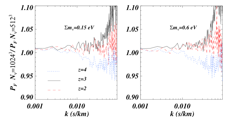
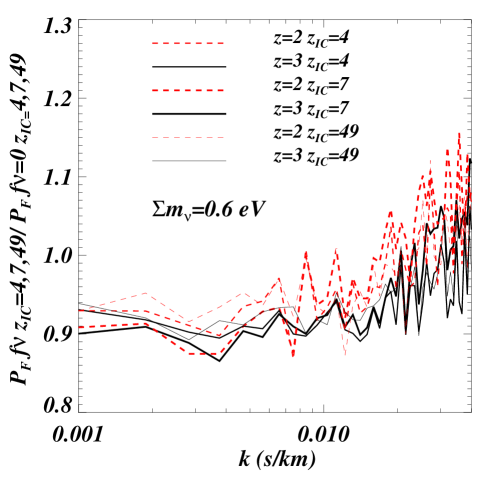
In Figure 18 we show the effect of varying the starting redshifts on the flux power spectrum ratios. The differences are significantly smaller than those for the matter power spectra (Figure 12). For neutrino masses with =0.6 eV the differences at and are at the level of 2% or less over the whole range of relevant wavenumbers (note that curves of the same color should be compared with each other).
The flux power spectrum of our simulation at appears to have converged at the 2% level in the range s/km. This level of numerical convergence should be sufficient for the analysis of presently available high- or low-resolution Lyman- forest data. The SDSS Lyman- flux power spectrum has statistical errors of the order of 3% or more at the smallest scales, and up to 10-15% at the largest scales, while the statistical errors of the high-resolution data are about two times larger than these.
4.3 Grid based vs particle based simulations of the effect of neutrinos on Lyman- forest data
We now have a closer look at the relative merits of grid based and particle based simulation on scales relevant for Lyman- forest data especially with regard to the Lyman- flux power spectrum. We will show how the differences shown in Figure 2 for the matter power spectra propagate to the flux power spectrum. In the left panel of Figure 19 we show the suppression of the matter power spectrum due to the free-streaming of neutrinos with =0.6 eV model on the matter power for simulations with the grid based implementation of the neutrino density. The suppression is larger than that of the corresponding simulation with the particle based neutrino implementation by about 10% (the horizontal green thick line indicates a value of ). In the middle panel, we directly compare the two implementations and while it is evident that at still linear scales, /Mpc, the agreement is at the 2% level, at smaller scales the differences are larger, about 7% at . In the rightmost panel, we compare the two implementations in terms of (one-dimensional) flux power. In this case the differences are of the order of for the scales considered in here. On the scales relevant for the Lyman- forest data the non-linear evolution of the matter distribution is more important than the effect of the Poisson contribution to the neutrino power spectrum justifying our choice of the particle based implementation for a quantitative analysis.

5 An upper limit on the neutrino mass from the SDSS Lyman- forest data
5.1 The SDSS flux power spectrum
We now turn to deriving an upper limit on the neutrino mass from the SDSS Lyman- forest data for which the flux power spectrum has been measured by [51]. This unique data set consists of 3035 absorption spectra of quasars in the redshift range , drawn from the DR1 and DR2 data releases. Since the spectral resolution is , the typical Lyman- absorption features with a width of km/s are not resolved. The signal-to-noise of the individual spectra is rather low, S/N per pixel. Due to the large number of spectra the flux power spectrum on scales a factor of a few larger than the thermal cut-off can, however, be measured with small statistical errors.
Ref. [51] have re-analyzed the raw data and have extensively investigated the effect of noise, resolution of the spectrograph, sky subtraction, quasar continuum and associated metal absorption: corrections for these effects are made and estimates of the associated errors are given. The noise contribution to the flux power spectrum rises from 15-30 percent at the smallest wavenumbers to order unity at the largest wavenumbers and varies with redshift. The correctios for uncorrelated metal absorption are generally a factor five to ten smaller than this. The correction for resolution varies from 1% at the smallest wavenumbers to a factor four at the largest wavenumbers. As final result of their analysis, [51] present their estimate for the flux power spectrum at 12 wavenumbers in the range (s/km), equally spaced in for , 2.4, 2.6, 2.8, 3.0, 3.2, 3.4, 3.6, 3.8, 4.0, and 4.2, for a total of 132 data points. They also provide the covariance matrix. Here, we will use this flux power spectrum together with the recommended corrections to the data and the recommended treatment of the errors of these corrections.
We note that Ref. [40] has interpreted this flux power spectrum previously based on a set of numerical simulations giving a measurement of the linear matter power spectrum at and s/km. Due to the wide redshift range sampled, many degeneracies between cosmological and astrophysical parameters can be broken, allowing for a high precision measurement of the linear power spectrum at small scales.
5.2 Multi-dimensional likelihood analysis
In order to explore the multi-dimensional astrophysical and cosmological parameter space we will use an improved version of a method based on a Taylor expansion of the flux power spectrum around a fiducial model as presented in Ref. [31]. Note that this is an approximate approach that assumes a physically motivated best-guess model and allows an exploration of the likelihood function around it. If we denote with an arbitrary vector of astrophysical, cosmological and noise-related parameters close to the best-guess model described by , we assume that:
| (5) |
where are the components of the vector , which represent the astrophysical and cosmological parameters. We perform here the Taylor expansion to second order for each parameter independently (i.e. neglecting cross derivatives). To obtain the derivatives of the flux power spectrum we run a suite of hydrodynamical simulations changing one parameter at a time with respect to those of the best-guess model and keeping all other parameters fixed. We then calculate the first and second order coefficients according to equation (5). This procedure is performed for the astrophysical parameters describing the thermal state of the IGM, and (both described by a power-law at with three parameters each: amplitude at , and power-law indices for and ), the mean flux level (amplitude and slope) and the reionization redshift; and for the cosmological parameters in a flat CDM model (, , , , ) that affect the growth of structure.
We then use a Monte-Carlo Markov Chain technique based on a suitable modification of the publicly available COSMOMC code [52]. We thereby allow for parameters that describe noise, resolution and those that model the contribution of Damped Lyman- systems to the flux power spectrum. In total a set of 28 parameters are allowed to vary. For a more extensive discussion on the use of the MCMC method in this context we refer to [53, 54, 55].
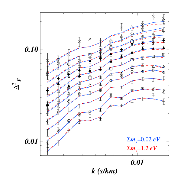
The main difference to our previous work in this respect is the addition of the effect of the neutrino mass on the flux power spectrum. Our analysis here does thereby not rely on any additional data which independently constrains the amplitude of the matter power spectrum on large scales. The results obtained in the previous sections refer to simulations that have a different and than our best-guess model (). We have thus rescaled the flux power spectrum to adjust for the different value of , .
The effect of the free-streaming of the neutrinos for a fixed value of is a small additional scale dependent suppression of the flux power which depends on redshift and mass of the neutrinos. The difference between the thick and thin curves in Figure 6 shows the effect for the matter power spectrum. Comparison of Figure 15 with Figure 16 shows that the corresponding effect on the flux power spectrum is somewhat smaller.
In order to demonstrate the effect of different values on the flux power spectrum we compare the theoretical predictions directly with the SDSS data points in Figure 20. Two different models are shown: the best fit model to the data with =0.02 eV and the same model (i.e. all the parameters fixed to the same values) but with a different =1.2 eV. The constraining power is largest for the data points at small scale and high redshift, similar to studies which constrain the free-streaming by warm dark matter particles.
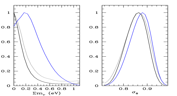
Our results with regard to the upper limit on the mass of neutrinos are summarized in Figure 21, where the one-dimensional marginalized (continuous curves) and mean (dashed curves) likelihoods for and are shown in the left and right panels, respectively. The constraints are (1 error bars) and eV (2 confidence level). The value for is in good agreement with previous analyses (e.g. [31]). We stress again that the constraint on is obtained from the SDSS flux power spectrum alone without considering other external data sets. The -value for the best fit model is 138.3 for 129 degrees of freedom, which should occur with a probability of 11%. We regard this upper limit as a conservative one, since having used the results obtained with the grid based approach would have produced a lower value than the one presented here, being the neutrino induced suppression larger for grid based simulations.
We note that the likelihoods in Figure 21 stay somewhat flat even for values eV, meaning that these values are allowed by SDSS data at the 2-2.5 level. In this Figure the mean likelihood is represented by the dotted curve, while the marginalized one is shown as a continuous curve. Note that this is very different from the result of the analysis in [9], where a very low upper limit of =0.17 eV was obtained. There are, however a number of important differences to our study here. The study of [9], is based on: inferring the linear dark matter power spectrum with a suite of approximate hydrodynamical simulations that do not incorporate neutrinos; and combining this measurement with other large scale structure probes. As extensively discussed in [9] the tension between the high r.m.s. values for the amplitude of the matter power spectrum suggested by Lyman- data and the lower values inferred from cosmic microwave background experiments is the main reason for the very low limit on .
It is also interesting to compare our findings with those that would be obtained by not considering the additional non-linear effects in simulations including neutrinos on the shape of the Lyman- flux power spectrum. The effect on the flux power spectrum can in this case be captured by the degenerate effect of changing the value of . In order to investigate this, we first add an extra parameter to represent neutrino’s mass fraction in the markov chains, which has exactly the same flux derivatives of the corresponding value, and then vary it independently from the others obtaining eV ( C.L). The results are shown in Figure 21 and one can see that the hold method results in a tighter upper bound because the likelihood is less flat for large values than in the new method (the upper limits are 0.38 eV and 0.18 eV for the old and new method, respectively). With this approximation the constraints are thus only slightly tighter than if we use the results from simulations including neutrinos which take the full non-linear effects on the shape of the flux power spectrum into account. The upper limit obtained in this way is also comparable to the constraint derived by just mapping (a-posteriori) the lower limit on , into an upper limit on using the code CAMB. In this latter case, however, and are not treated as independent parameters as they should if the matter power spectrum is normalized at the Lyman- forest scales. We think that the somewhat tigther constraints obtained without the results from the numerical simulations including neutrinos is due to the method we used. With the Taylor-expansion method we model small departures from a best-guess case and this is more accurately described by implementing the exact results on the flux power from the numerical simulations rather than treating the effect of and independently (in this second case the flux power is less likely to depart significantly from the reference case than in the first case). However, given the small difference between the two methods we would not regard this discrepancy as particularly significant.
We have focused here instead on investigating the impact of neutrinos on the (non-linear) spatial distribution of the neutral hydrogen in the IGM and the resulting flux power spectrum and obtaining a consistent upper limit on neutrino masses from the SDSS flux power spectrum alone. The rather small but scale dependent and redshift dependent impact of neutrinos with eV at the 4-5% level already results in an interesting upper limit which is somewhat stronger than that from the CMB data alone.
6 Summary and Discussion
Lyman- forest data in combination with cosmic microwave background measurements provide presently the lowest upper limits on the masses of neutrinos. A careful assessment of the ability of Lyman- forest data and in particular the Lyman- flux power spectrum to put limits on the effect of the free-streaming of neutrinos on the matter distribution is therefore important. The use of Lyman- forest data for measurements of the matter power spectrum relies heavily on the accurate modeling of the spatial distribution of neutral hydrogen. We have presented here for the first time a study of a large suite of hydrodynamical cosmological simulations that allow a quantification of the impact of neutrinos on the non-linear matter distribution as probed by the Intergalactic Medium. The simulations were performed with a modified version of GADGET-3 in which we have incorporated the effect of neutrinos by using a particle and a grid based method.
We have investigated a wide range of numerical issues relevant to simulating the effect of the free-streaming of neutrinos on the matter distribution. We find that with a particle based implementation the spatial distribution of the fast moving neutrinos suffers significantly from Poisson noise. On scales of interest for the use of Lyman- forest data the corresponding errors are, however, still smaller than the measurement errors of the flux power spectrum. The less CPU and memory demanding grid based implementation of neutrinos on the other hand does not suffer from Poisson noise but results in errors in the matter/flux power spectrum due to the assumption of linear theory for the growth of perturbations in the neutrino density. The error in the flux power spectrum in this case is as large as 4%, larger or comparable to the measurement errors. At linear scales Mpc simulations with the two different neutrino implementations agree at the 2% level at and at the 1% level at . The impact of other numerical effects investigated (starting redshift, velocities of the neutrino particles in the initial conditions) is also smaller or comparable to the statistical errors of the SDSS flux power spectrum.
By extracting a set of realistic mock quasar spectra, we quantify the effect of neutrinos on the flux probability distribution function and flux power spectrum. The free-streaming of neutrinos results in a (non-linear) scale-dependent suppression of the power spectrum of the total matter distribution at scales probed by Lyman- forest data which is larger than the linear theory prediction by about 25 % and strongly redshift dependent. The differences in the matter power spectra translate into a () difference in the flux power spectrum for neutrino masses with eV (0.6 eV).
We have performed a detailed comparison between simulations including neutrinos and simulations without neutrinos with a reduced overall amplitude of the matter power spectrum in order to disentangle as much as possible the effect of the free-streaming of neutrinos on the shape of the flux power spectrum and its evolution from the overall suppression of the power spectrum due to the free-streaming. The latter is responsible for the well known degeneracy between the (upper limit for the) mass of neutrinos and the value of . Breaking this degeneracy is important for a reliable assessment of the robustness of the upper limits on neutrino masses from Lyman- forest data as the lowest upper limits are based on combining measurements of the matter power spectrum on different scales with very different methods.
We find that the differences in the flux power spectrum and the flux probability distribution function between simulations including neutrinos and simulations without neutrinos with a reduced overall amplitude of the matter power spectrum are small but noticeable. Motivated by our findings, we then investigated whether the present SDSS data set alone can give constraints on the neutrino masses. We have explored the multi-dimensional likelihood space using the flux derivative method proposed by [31]. We found a conservative upper limit of = 0.9 eV at the level, obtained from SDSS quasar spectra alone, which is comparable to limits obtained with other probes of large scale structure. This limit is of course much weaker than published constraints obtained by combining Lyman- forest data with information from large scales, because the latter leverages the different r.m.s. value for the amplitude of the matter power spectrum suggested by small-scale and large-scale observables and turns this into a tight constraint for the absolute neutrino masses. The robustness of these recently published relatively low upper limits depends, however, strongly on the somewhat questionable assumption that there are no systematic offsets between the measurements obtained on small and large scales with these very different methods which are not yet fully understood or not correctly taken into account in the error analysis.
We have demonstrated here that a quantitative investigation of the effect of the free-streaming of neutrinos on the non-linear matter distribution as probed by the IGM structures can be efficiently performed with numerical hydrodynamical simulations. Reaching an accuracy below the one percent level at scales relevant for Lyman- forest or weak lensing data will still be challenging but should be doable and will be an important step in turning the exciting prospect of an actual measurement of neutrino masses into reality.
Acknowledgments.
We thank the referee for a useful and constructive report. MV is partly supported by ASI/AAE, INFN-PD51 and a PRIN by MIUR. Numerical computations were performed using the COSMOS Supercomputer in Cambridge (UK), which is sponsored by SGI, Intel, HEFCE and the Darwin Supercomputer of the University of Cambridge High Performance Computing Service (http://www.hpc.cam.ac.uk/), provided by Dell Inc. using Strategic Research Infrastructure Funding from the Higher Education Funding Council for England. Part of the analysis has been performed at CINECA with a Key project on the intergalactic medium obtained through a CINECA/INAF grant.References
- [1] J. Lesgourgues and S. Pastor, Massive neutrinos and cosmology, Physics Reports 429 (July, 2006) 307–379, [astro-ph/].
- [2] G. L. Fogli, E. Lisi, A. Marrone, A. Melchiorri, A. Palazzo, A. M. Rotunno, P. Serra, J. Silk, and A. Slosar, Observables sensitive to absolute neutrino masses. II, Phys. Rev. D 78 (Aug., 2008) 033010–+, [arXiv:0805.2517].
- [3] C. Ma and E. Bertschinger, Cosmological Perturbation Theory in the Synchronous and Conformal Newtonian Gauges, ApJ 455 (Dec., 1995) 7–+, [astro-ph/].
- [4] J. R. Bond, G. Efstathiou, and J. Silk, Massive neutrinos and the large-scale structure of the universe, Physical Review Letters 45 (Dec., 1980) 1980–1984.
- [5] R. A. C. Croft, D. H. Weinberg, M. Bolte, S. Burles, L. Hernquist, N. Katz, D. Kirkman, and D. Tytler, Toward a Precise Measurement of Matter Clustering: Ly Forest Data at Redshifts 2-4, ApJ 581 (Dec., 2002) 20–52, [astro-ph/].
- [6] M. Viel, M. G. Haehnelt, and V. Springel, Inferring the dark matter power spectrum from the Lyman forest in high-resolution QSO absorption spectra, MNRAS 354 (Nov., 2004) 684–694, [astro-ph/].
- [7] A. A. Meiksin, The physics of the intergalactic medium, Reviews of Modern Physics 81 (Oct., 2009) 1405–1469.
- [8] R. A. C. Croft, W. Hu, and R. Davé, Cosmological Limits on the Neutrino Mass from the Ly Forest, Physical Review Letters 83 (Aug., 1999) 1092–1095, [astro-ph/].
- [9] U. Seljak, A. Slosar, and P. McDonald, Cosmological parameters from combining the Lyman- forest with CMB, galaxy clustering and SN constraints, Journal of Cosmology and Astro-Particle Physics 10 (Oct., 2006) 14–+, [astro-ph/].
- [10] Ø. Elgarøy, O. Lahav, W. J. Percival, J. A. Peacock, D. S. Madgwick, S. L. Bridle, C. M. Baugh, I. K. Baldry, J. Bland-Hawthorn, T. Bridges, R. Cannon, S. Cole, M. Colless, C. Collins, W. Couch, G. Dalton, R. de Propris, S. P. Driver, G. P. Efstathiou, R. S. Ellis, C. S. Frenk, K. Glazebrook, C. Jackson, I. Lewis, S. Lumsden, S. Maddox, P. Norberg, B. A. Peterson, W. Sutherland, and K. Taylor, New Upper Limit on the Total Neutrino Mass from the 2 Degree Field Galaxy Redshift Survey, Physical Review Letters 89 (July, 2002) 061301–+, [astro-ph/].
- [11] M. Tegmark, D. J. Eisenstein, M. A. Strauss, D. H. Weinberg, M. R. Blanton, J. A. Frieman, M. Fukugita, J. E. Gunn, A. J. S. Hamilton, G. R. Knapp, R. C. Nichol, J. P. Ostriker, N. Padmanabhan, W. J. Percival, D. J. Schlegel, D. P. Schneider, R. Scoccimarro, U. Seljak, H. Seo, M. Swanson, A. S. Szalay, M. S. Vogeley, J. Yoo, I. Zehavi, K. Abazajian, S. F. Anderson, J. Annis, N. A. Bahcall, B. Bassett, A. Berlind, J. Brinkmann, T. Budavari, F. Castander, A. Connolly, I. Csabai, M. Doi, D. P. Finkbeiner, B. Gillespie, K. Glazebrook, G. S. Hennessy, D. W. Hogg, Ž. Ivezić, B. Jain, D. Johnston, S. Kent, D. Q. Lamb, B. C. Lee, H. Lin, J. Loveday, R. H. Lupton, J. A. Munn, K. Pan, C. Park, J. Peoples, J. R. Pier, A. Pope, M. Richmond, C. Rockosi, R. Scranton, R. K. Sheth, A. Stebbins, C. Stoughton, I. Szapudi, D. L. Tucker, D. E. vanden Berk, B. Yanny, and D. G. York, Cosmological constraints from the SDSS luminous red galaxies, Phys. Rev. D 74 (Dec., 2006) 123507–+, [astro-ph/].
- [12] A. Mantz, S. W. Allen, and D. Rapetti, The Observed Growth of Massive Galaxy Clusters IV: Robust Constraints on Neutrino Properties, ArXiv e-prints (Nov., 2009) [arXiv:0911.1788].
- [13] E. Komatsu, J. Dunkley, M. R. Nolta, C. L. Bennett, B. Gold, G. Hinshaw, N. Jarosik, D. Larson, M. Limon, L. Page, D. N. Spergel, M. Halpern, R. S. Hill, A. Kogut, S. S. Meyer, G. S. Tucker, J. L. Weiland, E. Wollack, and E. L. Wright, Five-Year Wilkinson Microwave Anisotropy Probe Observations: Cosmological Interpretation, ApJS 180 (Feb., 2009) 330–376, [arXiv:0803.0547].
- [14] E. Komatsu, K. M. Smith, J. Dunkley, C. L. Bennett, B. Gold, G. Hinshaw, N. Jarosik, D. Larson, M. R. Nolta, L. Page, D. N. Spergel, M. Halpern, R. S. Hill, A. Kogut, M. Limon, S. S. Meyer, N. Odegard, G. S. Tucker, J. L. Weiland, E. Wollack, and E. L. Wright, Seven-Year Wilkinson Microwave Anisotropy Probe (WMAP) Observations: Cosmological Interpretation, ArXiv e-prints (Jan., 2010) [arXiv:1001.4538].
- [15] B. A. Reid, L. Verde, R. Jimenez, and O. Mena, Robust neutrino constraints by combining low redshift observations with the CMB, Journal of Cosmology and Astro-Particle Physics 1 (Jan., 2010) 3–+, [arXiv:0910.0008].
- [16] S. A. Thomas, F. B. Abdalla, and O. Lahav, Upper Bound of 0.28eV on the Neutrino Masses from the Largest Photometric Redshift Survey, ArXiv e-prints (Nov., 2009) [arXiv:0911.5291].
- [17] S. Wang, Z. Haiman, W. Hu, J. Khoury, and M. May, Weighing Neutrinos with Galaxy Cluster Surveys, Physical Review Letters 95 (June, 2005) 011302–+, [astro-ph/].
- [18] S. Gratton, A. Lewis, and G. Efstathiou, Prospects for constraining neutrino mass using Planck and Lyman- forest data, Phys. Rev. D 77 (Apr., 2008) 083507–+, [arXiv:0705.3100].
- [19] A. Vallinotto, M. Viel, S. Das, and D. N. Spergel, Cross-correlations of the Lyman-alpha forest with weak lensing convergence I: Analytical Estimates of S/N and Implications for Neutrino Mass and Dark Energy, ArXiv e-prints (Oct., 2009) [arXiv:0910.4125].
- [20] A. Klypin, J. Holtzman, J. Primack, and E. Regos, Structure Formation with Cold plus Hot Dark Matter, ApJ 416 (Oct., 1993) 1–+, [astro-ph/].
- [21] C. Ma and E. Bertschinger, A calculation of the full neutrino phase space in cold + hot dark matter models, Astrophysical Journal 429 (July, 1994) 22–28, [astro-ph/].
- [22] J. Brandbyge, S. Hannestad, T. Haugbølle, and B. Thomsen, The effect of thermal neutrino motion on the non-linear cosmological matter power spectrum, Journal of Cosmology and Astro-Particle Physics 8 (Aug., 2008) 20–+, [arXiv:0802.3700].
- [23] J. Brandbyge and S. Hannestad, Grid based linear neutrino perturbations in cosmological N-body simulations, Journal of Cosmology and Astro-Particle Physics 5 (May, 2009) 2–+, [arXiv:0812.3149].
- [24] J. Brandbyge and S. Hannestad, Resolving Cosmic Neutrino Structure: A Hybrid Neutrino N-body Scheme, ArXiv e-prints (Aug., 2009) [arXiv:0908.1969].
- [25] J. Lesgourgues, S. Matarrese, M. Pietroni, and A. Riotto, Non-linear power spectrum including massive neutrinos: the time-RG flow approach, Journal of Cosmology and Astro-Particle Physics 6 (June, 2009) 17–+, [arXiv:0901.4550].
- [26] S. Saito, M. Takada, and A. Taruya, Nonlinear power spectrum in the presence of massive neutrinos: Perturbation theory approach, galaxy bias, and parameter forecasts, Phys. Rev. D 80 (Oct., 2009) 083528–+, [arXiv:0907.2922].
- [27] Y. Y. Y. Wong, Higher order corrections to the large scale matter power spectrum in the presence of massive neutrinos, Journal of Cosmology and Astro-Particle Physics 10 (Oct., 2008) 35–+, [arXiv:0809.0693].
- [28] S. Saito, M. Takada, and A. Taruya, Impact of Massive Neutrinos on the Nonlinear Matter Power Spectrum, Physical Review Letters 100 (May, 2008) 191301–+, [arXiv:0801.0607].
- [29] S. Hannestad, A. Ringwald, H. Tu, and Y. Y. Y. Wong, Is it possible to tell the difference between fermionic and bosonic hot dark matter?, Journal of Cosmology and Astro-Particle Physics 9 (Sept., 2005) 14–+, [astro-ph/].
- [30] K. Abazajian, E. R. Switzer, S. Dodelson, K. Heitmann, and S. Habib, Nonlinear cosmological matter power spectrum with massive neutrinos: The halo model, Phys. Rev. D 71 (Feb., 2005) 043507–+, [astro-ph/].
- [31] M. Viel and M. G. Haehnelt, Cosmological and astrophysical parameters from the Sloan Digital Sky Survey flux power spectrum and hydrodynamical simulations of the Lyman forest, MNRAS 365 (Jan., 2006) 231–244, [astro-ph/].
- [32] D. H. Rudd, A. R. Zentner, and A. V. Kravtsov, Effects of Baryons and Dissipation on the Matter Power Spectrum, ApJ 672 (Jan., 2008) 19–32, [astro-ph/].
- [33] T. Kim, M. Viel, M. G. Haehnelt, R. F. Carswell, and S. Cristiani, The power spectrum of the flux distribution in the Lyman forest of a large sample of UVES QSO absorption spectra (LUQAS), MNRAS 347 (Jan., 2004) 355–366, [astro-ph/].
- [34] V. Springel, The cosmological simulation code GADGET-2, MNRAS 364 (Dec., 2005) 1105–1134, [astro-ph/].
- [35] A. Lewis, A. Challinor, and A. Lasenby, Efficient computation of CMB anisotropies in closed FRW models, Astrophys. J. 538 (2000) 473–476, [astro-ph/9911177].
- [36] Y. B. Zel’Dovich, Gravitational instability: An approximate theory for large density perturbations., A&A 5 (Mar., 1970) 84–89.
- [37] F. R. Bouchet, S. Colombi, E. Hivon, and R. Juszkiewicz, Perturbative Lagrangian approach to gravitational instability., A&A 296 (Apr., 1995) 575–+, [astro-ph/].
- [38] M. Viel, J. S. Bolton, and M. G. Haehnelt, Cosmological and astrophysical constraints from the Lyman forest flux probability distribution function, MNRAS 399 (Oct., 2009) L39–L43, [arXiv:0907.2927].
- [39] J. Alimi, A. Füzfa, V. Boucher, Y. Rasera, J. Courtin, and P. Corasaniti, Imprints of dark energy on cosmic structure formation - I. Realistic quintessence models and the non-linear matter power spectrum, MNRAS 401 (Jan., 2010) 775–790, [arXiv:0903.5490].
- [40] P. McDonald, U. Seljak, R. Cen, D. Shih, D. H. Weinberg, S. Burles, D. P. Schneider, D. J. Schlegel, N. A. Bahcall, J. W. Briggs, J. Brinkmann, M. Fukugita, Ž. Ivezić, S. Kent, and D. E. Vanden Berk, The Linear Theory Power Spectrum from the Ly Forest in the Sloan Digital Sky Survey, Astrophysical Journal 635 (Dec., 2005) 761–783, [astro-ph/].
- [41] M. Viel, M. G. Haehnelt, and V. Springel, Testing the accuracy of the hydrodynamic particle-mesh approximation in numerical simulations of the Lyman forest, MNRAS 367 (Apr., 2006) 1655–1665, [astro-ph/].
- [42] M. Viel, S. Matarrese, H. J. Mo, M. G. Haehnelt, and T. Theuns, Probing the intergalactic medium with the Ly forest along multiple lines of sight to distant QSOs, MNRAS 329 (Feb., 2002) 848–862, [astro-ph/].
- [43] U. Seljak, A. Makarov, P. McDonald, and H. Trac, Can Sterile Neutrinos Be the Dark Matter?, Physical Review Letters 97 (Nov., 2006) 191303–+, [astro-ph/].
- [44] J. Wang and S. D. M. White, Discreteness effects in simulations of hot/warm dark matter, MNRAS 380 (Sept., 2007) 93–103, [astro-ph/].
- [45] L. Gao and T. Theuns, Lighting the Universe with Filaments, Science 317 (Sept., 2007) 1527–, [arXiv:0709.2165].
- [46] L. Hui and N. Y. Gnedin, Equation of state of the photoionized intergalactic medium, MNRAS 292 (Nov., 1997) 27–+, [astro-ph/].
- [47] T. Theuns, A. Leonard, G. Efstathiou, F. R. Pearce, and P. A. Thomas, P^3M-SPH simulations of the Lyalpha forest, MNRAS 301 (Dec., 1998) 478–502, [astro-ph/].
- [48] T. Kim, J. S. Bolton, M. Viel, M. G. Haehnelt, and R. F. Carswell, An improved measurement of the flux distribution of the Ly forest in QSO absorption spectra: the effect of continuum fitting, metal contamination and noise properties, MNRAS 382 (Dec., 2007) 1657–1674, [arXiv:0711.1862].
- [49] M. Viel, M. G. Haehnelt, R. F. Carswell, and T. Kim, The effect of (strong) discrete absorption systems on the Lyman forest flux power spectrum, MNRAS 349 (Apr., 2004) L33–L37, [astro-ph/].
- [50] J. Schaye, Model-independent Insights into the Nature of the Ly Forest and the Distribution of Matter in the Universe, ApJ 559 (Oct., 2001) 507–515, [astro-ph/].
- [51] P. McDonald, U. Seljak, S. Burles, D. J. Schlegel, D. H. Weinberg, R. Cen, D. Shih, J. Schaye, D. P. Schneider, N. A. Bahcall, J. W. Briggs, J. Brinkmann, R. J. Brunner, M. Fukugita, J. E. Gunn, Ž. Ivezić, S. Kent, R. H. Lupton, and D. E. Vanden Berk, The Ly Forest Power Spectrum from the Sloan Digital Sky Survey, ApJS 163 (Mar., 2006) 80–109, [astro-ph/].
- [52] A. Lewis and S. Bridle, Cosmological parameters from CMB and other data: A Monte Carlo approach, Phys. Rev. D 66 (Nov., 2002) 103511–+, [astro-ph/].
- [53] A. Boyarsky, J. Lesgourgues, O. Ruchayskiy, and M. Viel, Lyman- constraints on warm and on warm-plus-cold dark matter models, Journal of Cosmology and Astro-Particle Physics 5 (May, 2009) 12–+, [arXiv:0812.0010].
- [54] M. Viel, J. S. Bolton, and M. G. Haehnelt, Cosmological and astrophysical constraints from the Lyman forest flux probability distribution function, MNRAS 399 (Oct., 2009) L39–L43, [arXiv:0907.2927].
- [55] A. Lidz, C. Faucher-Giguere, A. Dall’Aglio, M. McQuinn, C. Fechner, M. Zaldarriaga, L. Hernquist, and S. Dutta, A Measurement of Small Scale Structure in the Lyman-alpha Forest, ArXiv e-prints (Sept., 2009) [arXiv:0909.5210].