On the road to percent accuracy III: non-linear reaction of the matter power spectrum to massive neutrinos

Abstract

We analytically model the non-linear effects induced by massive neutrinos on the total matter power spectrum using the halo model reaction framework of Cataneo et al. 2019. In this approach the halo model is used to determine the relative change to the matter power spectrum caused by new physics beyond the concordance cosmology. Using standard fitting functions for the halo abundance and the halo mass-concentration relation, the total matter power spectrum in the presence of massive neutrinos is predicted to percent-level accuracy, out to $k=10\,h\,{\rm Mpc}^{-1}$. We find that refining the prescriptions for the halo properties using $N$-body simulations improves the recovered accuracy to better than 1%. This paper serves as another demonstration for how the halo model reaction framework, in combination with a single suite of standard $\Lambda$CDM simulations, can recover percent-level accurate predictions for beyond-$\Lambda$CDM matter power spectra, well into the non-linear regime.

1 Introduction

In the standard model of particle physics, neutrinos are treated as elementary massless particles. However, it has been conclusively shown that neutrino flavour (i.e. electronic, muonic, tauonic) can change with time (Fukuda et al., 1998; Ahmed et al., 2004), a phenomenon know as flavour oscillations. For this to be possible, at least two neutrinos must possess a non-zero mass, therefore pointing to physics beyond the standard model. Since oscillation experiments measure the mass-squared splittings between the three mass eigenstates, they can only provide a lower bound on the absolute mass scale, and hence alone cannot determine the neutrino mass hierarchy (Qian & Vogel, 2015).

On the other hand, the presence of massive neutrinos has profound implications for the formation and evolution of structures in the Universe (Lesgourgues & Pastor, 2006). At early times, in particular at recombination, neutrinos are ultra-relativistic and so their masses do not affect the primary CMB. At redshifts of $\sim 200(m_{\nu}/0.1\,\mathrm{eV})$ neutrinos become non-relativistic; however, their still large thermal velocities prevent them from clustering strongly producing a characteristic modification to the matter power spectrum. Large-scale structure observables are therefore sensitive to the sum of neutrino masses (Marulli et al., 2011), with measurable effects, for instance, on the abundance of massive galaxy clusters (e.g. Costanzi et al., 2013) and two-point shear statistics (e.g., Liu et al., 2018).

Upcoming wide-field galaxy surveys will map the large-scale structure of the Universe to an unprecedented volume and accuracy (Laureijs et al., 2011; LSST Dark Energy Science Collaboration, 2012; Green et al., 2012; Levi et al., 2013), thus challenging our ability to predict cosmological summary statistics with the required small uncertainties over the entire range of relevant scales. In particular, percent-level knowledge of the matter power spectrum in the non-linear regime is necessary to take full advantage of future cosmic shear measurements (Taylor et al., 2018). At present, however, all known (semi-)analytical methods incorporating the non-linear effects of massive neutrinos on the matter power spectrum lack sufficient accuracy to be employed in future cosmological analyses aimed at stringent and unbiased constraints of the absolute mass scale (Bird et al., 2012; Blas et al., 2014; Mead et al., 2016; Lawrence et al., 2017).

In this paper we demonstrate how the halo model reaction framework of Cataneo et al. (2019) can predict the non-linear total matter power spectrum in the presence of massive neutrinos to the accuracy requirements imposed by the next generation of cosmological surveys. Sec. 2 describes our approach and the cosmological simulations used for its validation. Sec. 3 presents our results, and in Sec. 4 we discuss their implications and future applications.

Our baseline flat $\Lambda$CDM cosmology has total matter density $\Omega_{\rm m}=0.2905$, baryon density $\Omega_{\rm b}=0.0473$, reduced Hubble constant $h=0.6898$, scalar spectral index $n_{\rm s}=0.969$ and amplitude of scalar fluctuations $A_{\rm s}=2.422\times 10^{-9}$ at the pivot scale $k_{0}=0.002\,{\rm Mpc}^{-1}$. In massive neutrino cosmologies we fix all parameters to their baseline values, and vary the cold dark matter (CDM) density as $\Omega_{\rm c}=\Omega_{\rm m}-\Omega_{\rm b}-\Omega_{\nu}$, with $\Omega_{\nu}$ denoting the neutrino density. For our linear calculations we use the Boltzmann code camb (Lewis et al., 2000).

2 Methods

2.1 Halo model reactions with massive neutrinos

The implementation of massive neutrinos in the halo model (HM) has been previously studied in Abazajian et al. (2005) and Massara et al. (2014), with the latter finding inaccuracies as large as 20-30% in the predicted total matter non-linear power spectrum when compared to $N$-body simulations. To reduce these discrepancies down to a few percent, Massara et al. (2014) proposed the use of massive-to-massless neutrino HM power spectrum ratios. Here, we follow a similar strategy by extending the recently developed halo model reaction framework (Cataneo et al., 2019, also see Mead (2017) for its first applications) to include the effect of massive neutrinos. As we shall see in Sec. 3, this approach improves the halo model performance by more than one order of magnitude, therefore reaching the target accuracy set by the next generation of galaxy surveys, albeit neglecting baryonic feedback (Chisari et al., 2019).

The total matter power spectrum in the presence of massive neutrinos is given by the weighted sum

$$P^{\mathrm{(m)}}(k)=(1-f_{\nu})^{2}P^{\mathrm{(cb)}}(k)+2f_{\nu}(1-f_{\nu})P^{(\mathrm{cb}\nu)}(k)+f_{\nu}^{2}P^{(\nu)}(k)\,,$$ (1)

where $f_{\nu}=\Omega_{\nu}/\Omega_{\mathrm{m}}$, $P^{\mathrm{(cb)}}$ is the auto power spectrum of CDM+baryons, $P^{(\nu)}$ is the neutrino auto power spectrum, and $P^{(\mathrm{cb}\nu)}$ is the cross power spectrum of the neutrinos and the two other matter components. In our halo model predictions we approximate neutrino clustering as purely linear, allowing us to replace the neutrino non-linear auto power spectrum with its linear counterpart, $P_{\mathrm{L}}^{(\nu)}$, and thus rewrite the cross power spectrum as (Agarwal & Feldman, 2011; Ali-Haïmoud & Bird, 2013)

$$P_{\mathrm{HM}}^{(\mathrm{cb}\nu)}(k)\approx\sqrt{P_{\mathrm{HM}}^{\mathrm{(cb)}}(k)P_{\mathrm{L}}^{(\nu)}(k)}\,.$$ (2)

The CDM+baryons auto power spectrum is then divided into two-halo and one-halo contributions (see, e.g., Cooray & Sheth, 2002),

$$P_{\mathrm{HM}}^{\mathrm{(cb)}}(k)=P_{\mathrm{L}}^{\mathrm{(cb)}}(k)+P_{1\mathrm{h}}^{\mathrm{(cb)}}(k)\,,$$ (3)

where we neglect the two-halo integral pre-factor involving the linear halo bias (see Cataneo et al., 2019, for details).

In the reaction approach described in Cataneo et al. (2019), we must now define a pseudo massive neutrino cosmology, which is a flat and massless neutrino $\Lambda$CDM cosmology whose linear power spectrum is identical to the total linear matter power spectrum of the real massive neutrino cosmology at a chosen final redshift, $z_{\mathrm{f}}$, that is

$$P_{\mathrm{L}}^{\mathrm{pseudo}}\left(k,z_{\mathrm{f}}\right)=P_{\mathrm{L}}^{\mathrm{(m)}}\left(k,z_{\mathrm{f}}\right)\,.$$ (4)

Owing to the different linear growth in the two cosmologies, $P_{\mathrm{L}}^{\mathrm{pseudo}}$ and $P_{\mathrm{L}}^{\mathrm{(m)}}$ can differ substantially for $z>z_{\mathrm{f}}$. In the halo model language, the ratio of the real to pseudo non-linear total matter power spectra, i.e. the reaction, takes the form

$$\mathcal{R}(k)=\frac{(1-f_{\nu})^{2}P_{\mathrm{HM}}^{\mathrm{(cb)}}(k)+2f_{\nu}(1-f_{\nu})P_{\mathrm{HM}}^{(\mathrm{cb}\nu)}(k)+f_{\nu}^{2}P_{\mathrm{L}}^{(\nu)}(k)}{P_{\mathrm{HM}}^{\mathrm{pseudo}}(k)}\,,$$ (5)

with

$$P_{\mathrm{HM}}^{\mathrm{pseudo}}(k)=P_{\mathrm{L}}^{\mathrm{(m)}}(k)+P_{\mathrm{1h}}^{\mathrm{pseudo}}(k)\,.$$ (6)

For a mass-dependent and spherically symmetric halo profile with Fourier transform $u(k,M)$, the one-halo term is given by the integral

$$P_{1\mathrm{h}}(k)=\int\mathrm{d}\ln M\,n(M)\left(\frac{M}{\bar{\rho}}\right)^{2}\left|u\left(k,M\right)\right|^{2}\,,$$ (7)

where

$$n(M)\equiv\frac{\mathrm{d}n}{\mathrm{d}\ln M}=\frac{\bar{\rho}}{M}\left[\nu f(\nu)\right]\frac{\mathrm{d}\ln\nu}{\mathrm{d}\ln M}$$ (8)

is the virial halo mass function, and we use the Sheth-Tormen multiplicity function (Sheth & Tormen, 2002)

$$\nu f(\nu)=A\sqrt{\frac{2}{\pi}q\nu^{2}}\left[1+\left(q\nu^{2}\right)^{-p}\right]\exp\left[-q\nu^{2}/2\right]\,,$$ (9)

with $\{A,q,p\}=\{0.3292,0.7665,0.2488\}$ (Despali et al., 2016). In Eqs. (8) and (9) the peak height $\nu(M,z)\equiv\delta_{\mathrm{coll}}(z)/\sigma(M,z)$, where $\delta_{\mathrm{coll}}$ is the redshift-dependent spherical collapse threshold, and

$$\sigma^{2}(R,z)=\int\frac{\mathrm{d}^{3}k}{(2\pi)^{3}}|\tilde{W}(kR)|^{2}P_{\mathrm{L}}(k,z)\,.$$ (10)

Here, $R=(3M/4\pi\bar{\rho})^{1/3}$, and $\tilde{W}$ denotes the Fourier transform of the top-hat filter.

For the halo profile in Eq. (7) we assume the Navarro-Frank-White (NFW) profile (Navarro et al., 1996) truncated at its virial radius $R_{\mathrm{vir}}=(3M/4\pi\bar{\rho}\Delta_{\mathrm{vir}})^{1/3}$, where $\Delta_{\mathrm{vir}}$ is the redshift- and cosmology-dependent virial spherical overdensity (see, e.g., Cataneo et al., 2019). In our NFW profiles calculations, we approximate the relation between the halo virial concentration and mass with the power law

$$c(M,z)=\frac{c_{0}}{1+z}\left[\frac{M}{M_{*}(z)}\right]^{-\alpha}\,,$$ (11)

where the characteristic mass, $M_{*}$, satisfies $\nu(M_{*},z)=1$, and we set the $c$-$M$ relation parameters to their standard values $c_{0}=9$ and $\alpha=0.13$ (Bullock et al., 2001).

For the evaluation of the one-halo term (Eq. 7) we use different comoving background matter densities, linear matter power spectra, and spherical collapse evolution in the real and pseudo cosmologies. More specifically, for the CDM+baryons component in the real cosmology we have

$$\bar{\rho} \rightarrow \bar{\rho}_{\mathrm{cb}}\,,$$ (12)

$$P_{\mathrm{L}} \rightarrow P_{\mathrm{L}}^{\mathrm{(cb)}}\,.$$ (13)

Then the equation of motion for the spherical collapse overdensity (see, e.g., Cataneo et al., 2019) is independent of mass and sourced only by the CDM+baryons Newtonian potential (cf. LoVerde, 2014); the flat $\Lambda$CDM background expansion is controlled by $\Omega_{\mathrm{m}}$. On the other hand, for the pseudo cosmology

$$\bar{\rho} \rightarrow \bar{\rho}_{\mathrm{m}}\,,$$ (14)

$$P_{\mathrm{L}} \rightarrow P_{\mathrm{L}}^{\mathrm{(m)}}\,,$$ (15)

while the spherical collapse dynamics is still governed by the standard $\Lambda$CDM equation with $\Omega_{\mathrm{cb}}^{\rm pseudo}=\Omega_{\mathrm{m}}^{\rm real}$.

Finally, assuming we can accurately compute the non-linear matter power spectrum of the pseudo cosmology with methods other than the halo model (see, e.g., Giblin et al., 2019), the total matter power spectrum of the real cosmology, Eq. (1), can be rewritten in the halo model reaction framework as

$$P^{\mathrm{(m)}}(k,z)=\mathcal{R}(k,z)\times P^{\rm{pseudo}}(k,z)\,.$$ (16)

In this work we generally use the pseudo matter power spectrum measured from the simulations described in the next Section. However, to test the robustness of the reaction approach to alternative $N$-body codes implementing massive neutrinos, in Sec. 3.3 we employ Bird et al. (2012) and Takahashi et al. (2012) fitting formulas as proxy for the real and pseudo massive neutrino simulations, respectively.

2.2 $N$-body simulations

We compute our fiducial non-linear power spectra and halo properties with the publicly available $N$-body code cubep³m (Harnois-Déraps et al., 2013), which has been modified to include neutrinos as a separate set of particles (Inman et al., 2015; Emberson et al., 2017). We run a suite of simulations both with and without neutrino particles. In the standard massless neutrino case, particles are initialized from the Zel’dovich displacement field (Zel’Dovich, 1970), obtained from the combined baryons + CDM transfer functions, linearly evolved from $z=0$ to $z=100$. However, for the pseudo cosmologies we generate the initial conditions from the total linear matter power spectrum of the corresponding real massive neutrino cosmologies at $z_{\mathrm{f}}=0$ or 1 (see Eq. 4), rescaled to the initial redshift $z=100$ with the $\Lambda$CDM linear growth function using $\Omega_{\rm m}^{\rm real}$.

In the massive neutrino case the simulations run in two phases, as unphysical dynamics sourced by the large thermal velocities (such as unaccounted for relativistic effects or large Poisson fluctuations) can occur if neutrinos are included at too high redshift (Inman et al., 2015). In the first, from $z=100$ to $z=10$, only CDM particles are evolved; the neutrinos are treated as a perfectly homogeneous background component. We account for their impact on the growth factor by multiplying a $z=10$ CDM transfer function with the neutrino correction, $D(z=100)/D(z=10)$, where $D(a)\propto a^{1-3f_{\nu}/5}$ (Bond et al., 1980). The Zel’dovich displacement is also modified to account for neutrino masses, with every velocity component being multiplied by $1-3f_{\nu}/5$. Finally, the mass of every particle is multiplied by $1-f_{\nu}$. With this strategy, CDM perturbations are correct at $z=10$ even though we do not evolve neutrino perturbations before then. In the second phase, neutrinos are added into the code as a separate $N$-body species. For their initialization, neutrino density and velocity fields are computed at $z=10$ from camb transfer functions, and the Zel’dovich approximation is again used to compute particle displacements and velocities. A random thermal contribution, drawn from the Fermi-Dirac distribution, is also added to their velocities. cubep$3$m then co-evolves neutrinos and dark matter with masses weighted by $f_{\nu}$ and $1-f_{\nu}$ respectively.

In all neutrino runs, we assume a single massive neutrino contributing $\Omega_{\nu}h^{2}=m_{\nu}/93.14\,{\rm eV}$ (Mangano et al., 2005), and consider cosmologies with $m_{\nu}=0.05,0.1,0.2,0.4$ eV. We perform runs with $N_{\nu}=3072^{3}$ neutrino particles and box sizes $L_{\rm box}=500\,h^{-1}{\rm Mpc}$ for all values of $m_{\nu}$ considered, as well as one set of large-volume runs with $L_{\rm box}=1000\,h^{-1}{\rm Mpc}$ and $m_{\nu}=0.4$ eV. We use $N_{\rm cb}=1536^{3}$ CDM particles in the smaller boxes and $N_{\rm cb}=3072^{3}$ particles in the larger boxes, corresponding to a common mass resolution of $m_{\mathrm{cb}}=2.78\times 10^{9}\,h^{-1}M_{\odot}$ for the baseline $\Lambda$CDM cosmology. A common gravitational softening length of $24\,h^{-1}{\rm kpc}$ is also used.

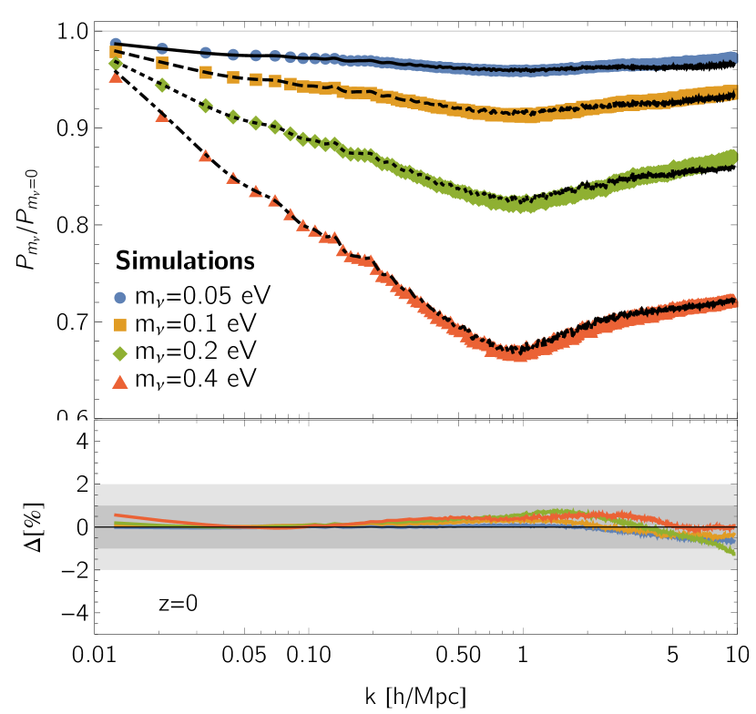
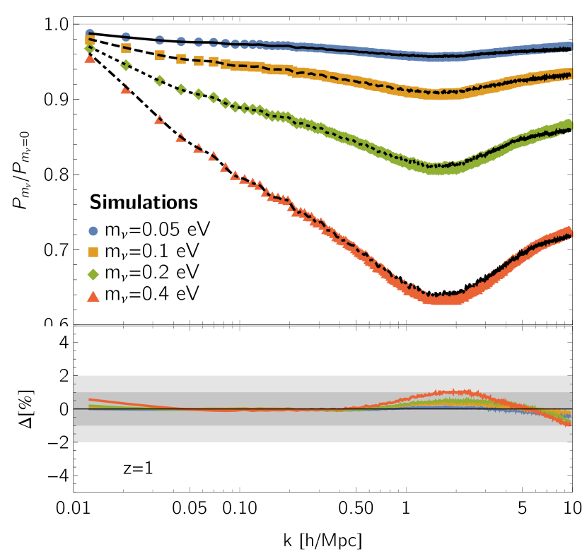
Figure 1: Total matter power spectrum ratios of the massive to the massless neutrino cosmologies at $z=0$ (left) and $z=1$ (right). The data points show the results of the $L_{\rm box}=500\,h^{-1}{\rm Mpc}$ simulations described in Sec. 2.2, and the black lines correspond to the halo model reaction predictions, $P^{\rm(m)}=\mathcal{R}\times P^{\rm pseudo}$, where $P^{\rm pseudo}$ is taken from flat $\Lambda$CDM dark matter-only simulations with pseudo initial conditions, and the halo model reactions are computed assuming the  Despali et al. (2016) and Bullock et al. (2001) fits for the halo mass functions and $c$-$M$ relations, respectively. The lower panels illustrate the excellent performance of our method, which matches the simulations at percent level for all $k\lesssim 10\,h\,{\rm Mpc}^{-1}$ (solid lines).

Halo catalogues for each simulation are generated using a spherical overdensity algorithm based on the method described in Harnois-Déraps et al. (2013). Briefly, the first stage of this process is to identify halo candidates as peaks in the dark matter density field. This is achieved by interpolating dark matter particles onto a uniform mesh with cell width $81\,h^{-1}{\rm kpc}$ and denoting candidates as local maxima in the density field. We then refine the density interpolation in the local region of each candidate using a mesh of width $16\,h^{-1}{\rm kpc}$ and identify a centre as the location of maximum density. The halo radius is defined by building spherical shells around the centre until the enclosed density reaches the cosmology- and redshift-dependent virial density, $\Delta_{\mathrm{vir}}$, derived from the spherical collapse and virial theorem. The density profile for each halo is stored using 20 logarithmically-spaced bins that reach out to $2\,h^{-1}{\rm Mpc}$. We compute a concentration for each halo by performing a least-squares fit to an NFW density profile. When doing so, we discard all radial bins smaller than twice the gravitational softening length and larger than the virial radius.

3 Results

3.1 $P^{\mathrm{(}m)}$ from the standard halo abundance and concentration fits

We begin by presenting the performance of the halo model reactions against our suite of small-volume simulations. For this comparison our reaction predictions (Eq. 5) are based on the standard values of the parameters entering the halo mass function (Despali et al., 2016) and $c$-$M$ relation (Bullock et al., 2001), which we apply to both the real and pseudo massive neutrino cosmologies. The upper panels of Fig. 1 shows the the impact of massive neutrinos on the non-linear total matter power spectrum for the range of neutrino masses relevant for the next generation of cosmological surveys (Coulton et al., 2019). The lower panels display the relative deviation of our predictions (see Eq. 16) from the full massive neutrino simulations, which is $\lesssim 1\%$ over the entire range of scales analysed and at both redshifts considered. This highly accurate result follows from the good agreement between the predicted real-to-pseudo halo mass function ratio and the simulations, which we show in the lower-left panel of Fig. 2 for the largest neutrino mass in our study. Cataneo et al. (2019) noticed that this quantity is directly related to the accuracy of the reaction across the transition to the non-linear regime. In fact, although the real and pseudo standard halo mass functions are a poor fit for halo masses $M\gtrsim 10^{14.5}\,h^{-1}M_{\odot}$ when taken individually (Fig. 2, upper- and middle-left panel), the predicted ratio remains within $\sim 2\%$ of the simulation measurements, thus corroborating the original findings of Cataneo et al. (2019). On the other hand, halo concentrations become relevant deep in the non-linear regime, and the right panel of Fig. 2 illustrates that despite the large absolute inaccuracies of the standard fits, once again the real-to-pseudo ratio is not too dissimilar from that of the simulations. This fact enables the excellent performance of the halo model reactions on scales $k\gtrsim 1\,h\,{\rm Mpc}^{-1}$.

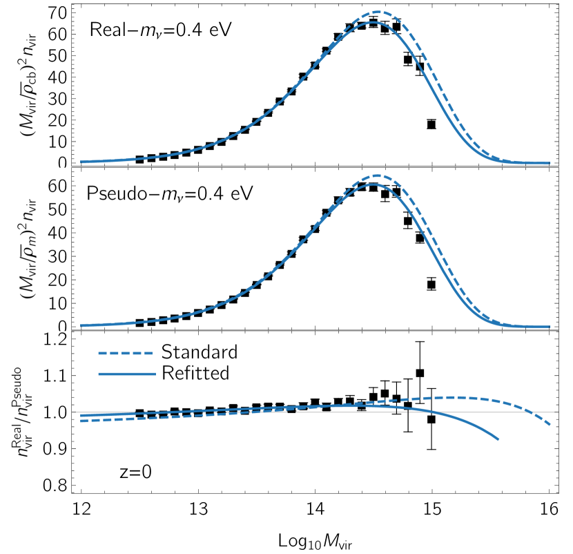
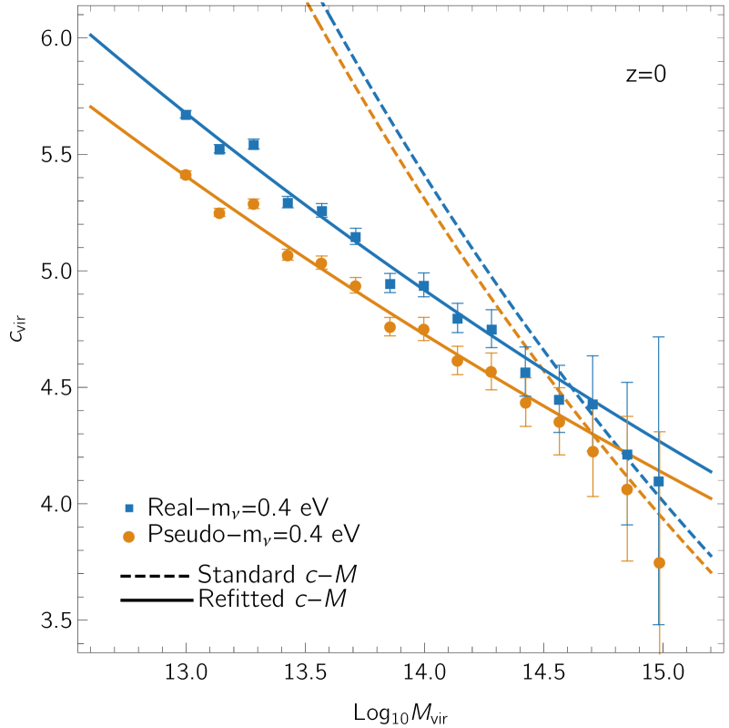
Figure 2: Halo properties extracted from the $z=0$ snapshots of the large-volume simulations ($L_{\rm box}=1000\,h^{-1}{\rm Mpc}$). Left: the abundance of dark matter halos for the real (top panel) and pseudo (middle panel) cosmologies with $m_{\nu}=0.4$ eV, both adjusted with prefactors such as to match the large-scale limit of the corresponding one-halo integrands (Eq. 7). The lower panel shows the real-to-pseudo halo mass function ratio, a quantity controlling the two-to-one-halo transition of the halo model reaction. The data points and error bars represent the means and Jackknife uncertainties obtained by splitting the simulation boxes in octants. Halo masses are binned in logarithmic bins of size $\Delta\log_{10}M=0.1$. We only use halos with more than 1000 particles and discard mass bins with fewer than 5 halos per sub-volume. The blue lines represent the Sheth-Tormen semi-analytical predictions with halo mass function parameters either taken from Despali et al. (2016) (dashed) or re-calibrated to fit individually our real and pseudo simulations (solid). Right: virial concentration-mass relation for the real (blue) and pseudo (orange) cosmologies with $m_{\nu}=0.4$ eV. The coloured lines are power law approximations with parameter values taken from Bullock et al. (2001) (dashed) or fitted to our simulations (solid). Symbols denote measurements from the simulations with central values corresponding to the mass-weighted mean concentration of the halos within each mass bin, and error bars only account for the Poisson noise. In addition, we only keep halos with more than 3000 particles to minimise profile fitting errors.

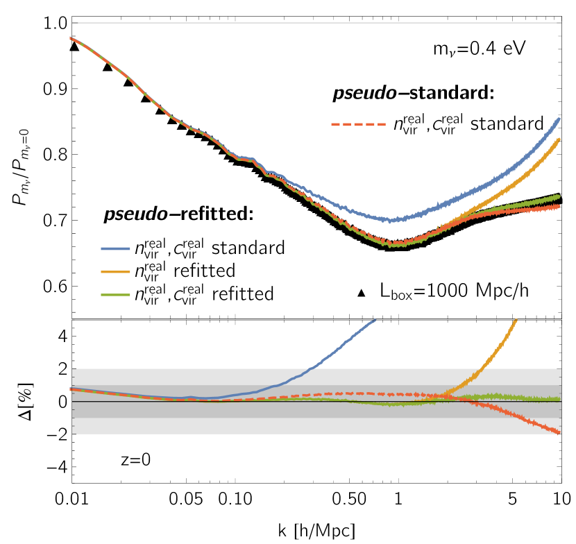
Figure 3: Present-day total matter power spectrum ratio of the massive neutrino cosmology with $m_{\nu}=0.4$ eV relative to the massless neutrino case. Symbols correspond to the measurements from the large-volume simulations. Solid lines are the halo model reaction predictions adopting the refitted halo mass functions and $c$-$M$ relations shown in Fig. 2 for the pseudo cosmology, while the real quantities use either the standard or refitted parameters. For comparison, we also show the predictions computed using the standard fits for both the pseudo and the real halo properties (dashed line). For all cases, our predictions use the non-linear matter power spectrum of the large-volume pseudo simulation. The lower panel shows that once the pseudo halo properties are calibrated to the simulations, the reaction enables an accurate one-to-one mapping between the real halo properties and the power spectrum, thus out-performing the traditional halo model calculations. Differences on small scales for the predictions based on the full standard fits (dashed line) compared to those in Fig. 1 are due to different halo concentrations in the small- and large-volume real massive neutrino simulations.

3.2 The effect of halo properties measured in simulations

It is currently unclear how accurately the non-linear matter power spectrum can be predicted given just mean halo properties such as their abundance and density profiles. For the standard halo model, it is well known that this approach fails due to large inaccuracies on quasi-linear scales of the absolute power spectrum (see, e.g., Giocoli et al., 2010; Massara et al., 2014). The halo model reactions, however, are fractional quantities, and as such better suited to absorb the errors incurred separately by the real and pseudo halo model predictions. To quantify the accuracy of this approach, we fit the Sheth-Tormen mass function and $c$-$M$ relations to our large volume $m_{\nu}=0.4$ eV simulations, obtaining $\{A^{\mathrm{real}},q^{\mathrm{real}},p^{\mathrm{real}}\}=\{0.3152,0.8423,0\}$, $\{A^{\mathrm{pseudo}},q^{\mathrm{pseudo}},p^{\mathrm{pseudo}}\}=\{0.3097,0.8313,0\}$, $\{c_{0}^{\mathrm{real}},\alpha^{\mathrm{real}}\}=\{6.3,0.062\}$, $\{c_{0}^{\mathrm{pseudo}},\alpha^{\mathrm{pseudo}}\}=\{6,0.058\}$. We show these fits as solid lines in Fig. 2.

To estimate the relative importance of the mean halo properties for the accuracy of the predicted non-linear power spectrum, in Fig. 3 we fix the pseudo halo mass function and $c$-$M$ parameters to their refitted values while varying their real counterparts. When the parameters entering the halo mass function and $c$-$M$ relation are all set to their standard values (blue line), our predictions experience deviations as large as $\sim 10\%$ for $k\gtrsim 0.1\,h\,{\rm Mpc}^{-1}$. The match to the simulations improves substantially on scales $0.1\lesssim k\lesssim 1\,h\,{\rm Mpc}^{-1}$ by including information on the halo mass function (orange line). If we further add our knowledge of the real halo concentrations, the agreement with the simulations reaches sub-percent level down to the smallest scales modelled in this study. These results confirm that the halo model reactions can produce even higher-quality predictions when supplied with accurate halo properties and pseudo non-linear power spectra. For comparison, we also show the calculation based on the standard fits for both the pseudo and the real halo properties (dashed line). Differences on scales $k\gtrsim 5\,h\,{\rm Mpc}^{-1}$ compared to the same prediction in Fig. 1 are primarily sourced by changes to the concentrations of small halos between the small- and large-volume simulations of the real massive neutrino cosmology, which in turn depend on the different $N_{\nu}/N_{\rm cb}$ particle number ratio used for these two runs (see Sec. 2.2).

3.3 Comparison to halofit

We shall now assess the validity of the halo model reactions for alternative implementations of the gravitational force (e.g. Springel, 2005; Habib et al., 2016) and of massive neutrinos (e.g. Banerjee & Dalal, 2016; Bird et al., 2018) in $N$-body codes. Ideally, we would carry out this test using the simulation outputs of codes other than cubep³m (e.g., Castorina et al., 2015; Liu et al., 2018). However, publicly available snapshots do not include runs for the pseudo cosmologies, which means we must resort to our simulations for these cases. Given that the clustering of matter generated by different codes can vary considerably even for dark matter-only simulations (Schneider et al., 2016; Garrison et al., 2019), this choice could bias our conclusions in the highly non-linear regime. Instead, we use halofit to compute the non-linear matter power spectrum, employing the Takahashi et al. (2012) calibration for the pseudo and the massless $\Lambda$CDM cases, and the Bird et al. (2012) prescription for the massive neutrino cosmologies; these two fitting functions are calibrated to the output of gadget-2 and gadget-3 codes (Springel et al., 2001; Springel, 2005), respectively. Moreover, for this comparison we use the standard halo mass function and $c$-$M$ relation parameters listed in Sec. 2.1, i.e. without refitting to the cubep³m simulations. We find that our reaction-based predictions for the total matter power spectrum of the massive neutrino cosmologies deviate no more than 3% from the halofit outputs. Such departures are comparable to, or smaller than, the typical halofit inaccuracies (see, e.g., Knabenhans et al., 2019; Smith & Angulo, 2019), which suggests our method can also satisfactorily reproduce the results of other $N$-body codes provided that the baseline pseudo power spectrum is obtained from simulations run with the same code and initial random phases of their real massive neutrino counterparts.

4 Discussion

In this paper we incorporated in the halo model reaction framework of Cataneo et al. (2019) an effective analytical strategy to accurately describe the non-linear effects induced by massive neutrinos on the total matter power spectrum. Our approach draws from the cold dark matter prescription adopted in Massara et al. (2014), with the notable difference that here we treated the clustering of massive neutrinos as purely linear, and worked with pseudo rather than the standard massless neutrino cosmology as baseline in our halo model power spectrum ratios. In contrast to modified gravity cosmologies (Cataneo et al., 2019), we found that the inclusion of high-order perturbative corrections to the two-halo contributions in the reaction was unnecessary.

We studied the interdependency between halo properties and matter power spectrum reactions, and conclusively showed that accurate knowledge of the mean halo abundances and concentrations (both central in cluster cosmology studies) leads to exquisite predictions for the halo model reactions. Together with the fast emulation method to compute the pseudo non-linear matter power spectrum presented in Giblin et al. (2019), the tight connection between halo mass function and matter power spectrum in our approach enables, for instance, the simultaneous analysis of cluster number counts and cosmic shear data in a novel, self-consistent way. In a future work, we will merge in a single reaction function both massive neutrino and dark energy/modified gravity cosmologies, which will enable us to predict the combined effects of these extensions on the matter power spectrum in a regime so far only accessible to specially modified $N$-body simulations (Baldi et al., 2014; Giocoli et al., 2018; Wright et al., 2019).

Finally, poorly understood baryonic processes impact the distribution of matter on scales $k\gtrsim 1\,h\,{\rm Mpc}^{-1}$, thus limiting our ability to correctly model the power spectrum deep in the non-linear regime (see Chisari et al., 2019, for a review). It was showed that it is possible to account for these additional effects within the halo model (Semboloni et al., 2011, 2013; Fedeli, 2014; Mohammed et al., 2014; Mead et al., 2015; Schneider et al., 2019; Debackere et al., 2019), and we leave the implementation of baryonic feedback in the halo model reactions to future investigation.

References

- Abazajian et al. (2005) Abazajian K., Switzer E. R., Dodelson S., Heitmann K., Habib S., 2005, Phys. Rev. D, 71, 043507
- Agarwal & Feldman (2011) Agarwal S., Feldman H. A., 2011, MNRAS, 410, 1647
- Ahmed et al. (2004) Ahmed S. N., et al., 2004, Phys. Rev. Lett., 92, 181301
- Ali-Haïmoud & Bird (2013) Ali-Haïmoud Y., Bird S., 2013, MNRAS, 428, 3375
- Baldi et al. (2014) Baldi M., Villaescusa-Navarro F., Viel M., Puchwein E., Springel V., Moscardini L., 2014, MNRAS, 440, 75
- Banerjee & Dalal (2016) Banerjee A., Dalal N., 2016, J. Cosmology Astropart. Phys., 2016, 015
- Behroozi et al. (2013) Behroozi P. S., Wechsler R. H., Wu H.-Y., 2013, ApJ, 762, 109
- Bird et al. (2012) Bird S., Viel M., Haehnelt M. G., 2012, MNRAS, 420, 2551
- Bird et al. (2018) Bird S., Ali-Haïmoud Y., Feng Y., Liu J., 2018, MNRAS, 481, 1486
- Blas et al. (2014) Blas D., Garny M., Konstandin T., Lesgourgues J., 2014, J. Cosmology Astropart. Phys., 2014, 039
- Bond et al. (1980) Bond J. R., Efstathiou G., Silk J., 1980, Phys. Rev. Lett., 45, 1980
- Bullock et al. (2001) Bullock J. S., Kolatt T. S., Sigad Y., Somerville R. S., Kravtsov A. V., Klypin A. A., Primack J. R., Dekel A., 2001, MNRAS, 321, 559
- Castorina et al. (2015) Castorina E., Carbone C., Bel J., Sefusatti E., Dolag K., 2015, J. Cosmology Astropart. Phys., 2015, 043
- Cataneo et al. (2019) Cataneo M., Lombriser L., Heymans C., Mead A. J., Barreira A., Bose S., Li B., 2019, MNRAS, p. 1778
- Chisari et al. (2019) Chisari N. E., et al., 2019, The Open Journal of Astrophysics, 2, 4
- Cooray & Sheth (2002) Cooray A., Sheth R., 2002, Phys. Rep., 372, 1
- Costanzi et al. (2013) Costanzi M., Villaescusa-Navarro F., Viel M., Xia J.-Q., Borgani S., Castorina E., Sefusatti E., 2013, J. Cosmology Astropart. Phys., 2013, 012
- Coulton et al. (2019) Coulton W. R., Liu J., Madhavacheril M. S., Böhm V., Spergel D. N., 2019, J. Cosmology Astropart. Phys., 2019, 043
- Debackere et al. (2019) Debackere S. N. B., Schaye J., Hoekstra H., 2019, arXiv e-prints, p. arXiv:1908.05765
- Despali et al. (2016) Despali G., Giocoli C., Angulo R. E., Tormen G., Sheth R. K., Baso G., Moscardini L., 2016, MNRAS, 456, 2486
- Elahi et al. (2019) Elahi P. J., Cañas R., Poulton R. J. J., Tobar R. J., Willis J. S., Lagos C. d. P., Power C., Robotham A. S. G., 2019, Publ. Astron. Soc. Australia, 36, e021
- Emberson et al. (2017) Emberson J. D., et al., 2017, Research in Astronomy and Astrophysics, 17, 085
- Fedeli (2014) Fedeli C., 2014, J. Cosmology Astropart. Phys., 2014, 028
- Fukuda et al. (1998) Fukuda Y., et al., 1998, Phys. Rev. Lett., 81, 1158
- Garrison et al. (2019) Garrison L. H., Eisenstein D. J., Pinto P. A., 2019, MNRAS, 485, 3370
- Giblin et al. (2019) Giblin B., Cataneo M., Moews B., Heymans C., 2019, arXiv e-prints, p. arXiv:1906.02742
- Giocoli et al. (2010) Giocoli C., Bartelmann M., Sheth R. K., Cacciato M., 2010, MNRAS, 408, 300
- Giocoli et al. (2018) Giocoli C., Baldi M., Moscardini L., 2018, MNRAS, 481, 2813
- Green et al. (2012) Green J., et al., 2012, arXiv e-prints, p. arXiv:1208.4012
- Habib et al. (2016) Habib S., et al., 2016, New Astron., 42, 49
- Harnois-Déraps et al. (2013) Harnois-Déraps J., Pen U.-L., Iliev I. T., Merz H., Emberson J. D., Desjacques V., 2013, MNRAS, 436, 540
- Inman (2017) Inman D., 2017, PhD thesis, University of Toronto (Canada)
- Inman et al. (2015) Inman D., Emberson J. D., Pen U.-L., Farchi A., Yu H.-R., Harnois-Déraps J., 2015, Phys. Rev. D, 92, 023502
- Knabenhans et al. (2019) Knabenhans M., et al., 2019, MNRAS, 484, 5509
- LSST Dark Energy Science Collaboration (2012) LSST Dark Energy Science Collaboration 2012, preprint, (arXiv:1211.0310)
- Laureijs et al. (2011) Laureijs R., et al., 2011, preprint, (arXiv:1110.3193)
- Lawrence et al. (2017) Lawrence E., et al., 2017, ApJ, 847, 50
- Lesgourgues & Pastor (2006) Lesgourgues J., Pastor S., 2006, Phys. Rep., 429, 307
- Levi et al. (2013) Levi M., et al., 2013, preprint, (arXiv:1308.0847)
- Lewis et al. (2000) Lewis A., Challinor A., Lasenby A., 2000, ApJ, 538, 473
- Liu et al. (2018) Liu J., Bird S., Zorrilla Matilla J. M., Hill J. C., Haiman Z., Madhavacheril M. S., Petri A., Spergel D. N., 2018, J. Cosmology Astropart. Phys., 2018, 049
- LoVerde (2014) LoVerde M., 2014, Phys. Rev. D, 90, 083518
- Loken et al. (2010) Loken C., et al., 2010, in Journal of Physics Conference Series. p. 012026, doi:10.1088/1742-6596/256/1/012026
- Mangano et al. (2005) Mangano G., Miele G., Pastor S., Pinto T., Pisanti O., Serpico P. D., 2005, Nuclear Physics B, 729, 221
- Marulli et al. (2011) Marulli F., Carbone C., Viel M., Moscardini L., Cimatti A., 2011, MNRAS, 418, 346
- Massara et al. (2014) Massara E., Villaescusa-Navarro F., Viel M., 2014, J. Cosmology Astropart. Phys., 12, 053
- McCarthy et al. (2018) McCarthy I. G., Bird S., Schaye J., Harnois-Deraps J., Font A. S., van Waerbeke L., 2018, MNRAS, 476, 2999
- Mead (2017) Mead A. J., 2017, MNRAS, 464, 1282
- Mead et al. (2015) Mead A. J., Peacock J. A., Heymans C., Joudaki S., Heavens A. F., 2015, MNRAS, 454, 1958
- Mead et al. (2016) Mead A. J., Heymans C., Lombriser L., Peacock J. A., Steele O. I., Winther H. A., 2016, MNRAS, 459, 1468
- Mohammed et al. (2014) Mohammed I., Martizzi D., Teyssier R., Amara A., 2014, arXiv e-prints, p. arXiv:1410.6826
- Navarro et al. (1996) Navarro J. F., Frenk C. S., White S. D. M., 1996, ApJ, 462, 563
- Ponce et al. (2019) Ponce M., et al., 2019, arXiv e-prints, p. arXiv:1907.13600
- Qian & Vogel (2015) Qian X., Vogel P., 2015, Progress in Particle and Nuclear Physics, 83, 1
- Schmidt (2016) Schmidt F., 2016, Phys. Rev. D, 93, 063512
- Schneider et al. (2016) Schneider A., et al., 2016, J. Cosmology Astropart. Phys., 2016, 047
- Schneider et al. (2019) Schneider A., Teyssier R., Stadel J., Chisari N. E., Le Brun A. M. C., Amara A., Refregier A., 2019, J. Cosmology Astropart. Phys., 2019, 020
- Semboloni et al. (2011) Semboloni E., Hoekstra H., Schaye J., van Daalen M. P., McCarthy I. G., 2011, MNRAS, 417, 2020
- Semboloni et al. (2013) Semboloni E., Hoekstra H., Schaye J., 2013, MNRAS, 434, 148
- Sheth & Tormen (2002) Sheth R. K., Tormen G., 2002, MNRAS, 329, 61
- Smith & Angulo (2019) Smith R. E., Angulo R. E., 2019, MNRAS, 486, 1448
- Springel (2005) Springel V., 2005, MNRAS, 364, 1105
- Springel et al. (2001) Springel V., Yoshida N., White S. D. M., 2001, New Astron., 6, 79
- Takahashi et al. (2012) Takahashi R., Sato M., Nishimichi T., Taruya A., Oguri M., 2012, ApJ, 761, 152
- Taylor et al. (2018) Taylor P. L., Kitching T. D., McEwen J. D., 2018, Phys. Rev. D, 98, 043532
- Wright et al. (2019) Wright B. S., Koyama K., Winther H. A., Zhao G.-B., 2019, J. Cosmology Astropart. Phys., 2019, 040
- Zel’Dovich (1970) Zel’Dovich Y. B., 1970, A&A, 500, 13