Enhancing the hierarchy and octant sensitivity of ESS$\nu$SB in conjunction with T2K, NO$\nu$A and ICAL@INO

Abstract

The main aim of the ESS$\nu$SB proposal is the discovery of the leptonic CP phase $\delta_{CP}~{}$with a high significance ($5\sigma$ for 50% values of $\delta_{CP}~{}$) by utilizing the physics at the second oscillation maxima of the $P_{\mu e}$ channel. It can achieve $3\sigma$ sensitivity to hierarchy for all values of $\delta_{CP}~{}$. In this work, we concentrate on the hierarchy and octant sensitivity of the ESS$\nu$SB experiment. We show that combining the ESS$\nu$SB experiment with the atmospheric neutrino data from the proposed India-based Neutrino Observatory(INO) experiment can result in an increased sensitivity to mass hierarchy. In addition, we also combine the results from the ongoing experiments T2K and NO$\nu$A assuming their full runtime and present the combined sensitivity of ESS$\nu$SB + ICAL@INO + T2K + NO$\nu$A. We show that while by itself ESS$\nu$SB can have up to $3\sigma$ hierarchy sensitivity, the combination of all the experiments can give up to $5\sigma$ sensitivity depending on the true hierarchy-octant combination. The octant sensitivity of ESS$\nu$SB is low by itself. However the combined sensitivity of all the above experiments can give up to $3\sigma$ sensitivity depending on the choice of true hierarchy and octant. We discuss the various degeneracies and the synergies that lead to the enhanced sensitivity when combining different experimental data.

1 Introduction

Several commendable ongoing and past experiments have not only established neutrino oscillation phenomenon, the oscillation parameters have also been quantified with considerable precision. In the three flavor framework, these are the mixing angles $\theta_{12}$, $\theta_{13}$, $\theta_{23}$ and the mass squared differences $\Delta m^{2}_{21}$, and $|\Delta m^{2}_{31}|$, where $\Delta m^{2}_{ij}=m_{i}^{2}-m_{j}^{2}$, $i,j=1,2,3~{}\&~{}i>j$. The unresolved parameters at this stage are the – neutrino mass hierarchy or the sign of $\Delta m^{2}_{31}$, octant of $\theta_{23}$ and the CP phase $\delta_{CP}$. The mass hierarchy or mass ordering depends on the position of the mass eigenstate state $m_{3}$ with respect to the other two. If $m_{3}>m_{2}>m_{1}$, then it is called Normal Hierarchy (NH) whereas if $m_{3}<m_{1}<m_{2}$ it is called Inverted Hierarchy (IH). As for the octant, $\theta_{23}<45^{\circ}$ implies Lower Octant (LO) and $\theta_{23}>45^{\circ}$ corresponds to the Higher Octant (HO). CP phase $\delta_{CP}$ is the parameter which governs the CP violation in the neutrino sector: $\delta_{CP}=0^{\circ},\pm 180^{\circ}$ implies CP conservation whereas $\delta_{CP}=\pm 90^{\circ}$ corresponds to maximum CP violation. Global analysis of data from all the neutrino oscillation experiments indicates $\delta_{CP}~{}$$\sim-90^{\circ}$, reports a hint for NH and a preference for HO Capozzi et al. (2017); Esteban et al. (2017); de Salas et al. (2018). One of the main difficulties in determining these parameters are the presence of degeneracies due to the unknown value of the phase $\delta_{CP}$. Several future experiments are proposed or planned to address the above degeneracies and unambiguous determination of the parameters – hierarchy, octant and $\delta_{CP}$. This includes the beam based experiments T2HK Abe et al. (2014) $/$ T2HKK Abe et al. (2016), DUNE Acciarri et al. (2015) and ESS$\nu$SB Baussan et al. (2012, 2014). Many studies have been performed in the literature to explore the physics potential of these facilities Agarwalla et al. (2014a); Ghosh et al. (2016a); Bora et al. (2015); Barger et al. (2014); Deepthi et al. (2015); Nath et al. (2016); Soumya et al. (2016); Coloma et al. (2013); Ballett et al. (2017); Agarwalla et al. (2017); Ghosh (2016); Ghosh and Yasuda (2017); Raut (2017); Das et al. (2018). A recent comparative study of these facilities have been accomplished in Chakraborty et al. (2018). Among these, the ESS$\nu$SB proposal plans to use the European Spallation Source (ESS), which is under construction in Sweden. The ESS$\nu$SB experiment will use this facility for generating a very intense neutrino super-beam. The main aim of the ESS$\nu$SB experiment is to measure the CP violation in the neutrino sector. This is expected to be achieved by using the second oscillation maxima of the $P_{\mu e}$ probability. However, for such a set-up the hierarchy and octant sensitivity gets compromised as compared to the first oscillation maximum. Optimization of the ESS$\nu$SB proposal for discovery of $\delta_{CP}~{}$has been done in Baussan et al. (2014), which recommends the neutrino baseline in the 300-550 km range and peak energy of 0.24 GeV. It was shown that $5\sigma$ sensitivity can be achieved for discovery of CP violation for 50% of the $\delta_{CP}~{}$values for 2 years of $\nu$ and 8 years of $\bar{\nu}$ run. This configuration can also reach $3\sigma$ hierarchy sensitivity for majority of the $\delta_{CP}~{}$values. In Agarwalla et al. (2014b) the octant sensitivity of ESS$\nu$SB has been studied at both first and second oscillation maxima and they advocated 200 km baseline with 7$\nu$+3$\bar{\nu}$ years as the optimal configuration for octant and CP sensitivity.

In this study our aim is to explore whether the hierarchy and octant sensitivity of ESS$\nu$SB can be improved by combining with the proposed atmospheric neutrino experiment ICAL@INOAhmed et al. (2017). It has been shown earlier that since the hierarchy sensitivity of ICAL@INO is independent of $\delta_{CP}$, combination of ICAL@INO with T2K and NO$\nu$A can help to raise the hierarchy sensitivity for unfavorable values of $\delta_{CP}~{}$for the latter experimentsChatterjee et al. (2013). We perform a quantitative analysis of this effect for the ESS$\nu$SB experiment. In addition we also explore how the information from the ongoing experiments T2K and NO$\nu$A can further enhance the hierarchy and octant sensitivity of the ESS$\nu$SB experiment as well as ESS$\nu$SB + ICAL@INO combination. We discuss in detail the various degeneracies and expound the synergistic effects of combining data from the various experiments. The ESS$\nu$SB set-up that we consider corresponds to that discussed in Baussan et al. (2014) with a baseline of 540 km – between Lund and Garpenberg mine.

This paper is structured as follows. In section 2, we have described the appearance probabilities of the long-baseline accelerator experiments (LBL) and the associated degeneracies. We also discuss briefly the behavior of the probability for baselines and energies for which resonance matter effect occurs for atmospheric neutrinos passing through the earth. Section 3, summarizes the various experiments that are used in this analysis and in section 4 the details of the simulation procedure is described. The section 5 contains the results for the mass hierarchy and octant sensitivity that can be achieved from ESS$\nu$SB , ICAL@INO , T2K + NO$\nu$A and their various combinations. Conclusions are presented in section 6.

2 Probability analysis

For the accelerator based experiments T2K, NO$\nu$A, ESS$\nu$SB the relevant channel for mass hierarchy and octant sensitivity is the appearance channel governed by the probability $P_{\mu e}$. In presence of matter of constant density, this can be expanded in terms of the small parameters $\alpha~{}(=~{}\frac{\Delta m^{2}_{21}}{\Delta m^{2}_{31}})$ and $\sin{\theta_{13}}$ up to second order as Akhmedov et al. (2004) :

$$P(\nu_{\mu}\rightarrow\nu_{e}) = \sin^{2}{2\theta_{13}}\sin^{2}{\theta_{23}}\frac{\sin^{2}{\Delta}(1-\hat{A})}{(1-\hat{A})^{2}}$$ (1)

$$+\alpha\cos{\theta_{13}}\sin{2\theta_{12}}\sin{2\theta_{13}}\sin{2\theta_{23}}\cos{(\Delta+\delta_{CP})}\frac{\sin{\Delta\hat{A}}}{\hat{A}}\frac{\sin{\Delta(1-\hat{A})}}{(1-\hat{A})}$$

$$+\alpha^{2}\sin^{2}{2\theta_{12}}\cos^{2}{\theta_{13}}\cos^{2}\theta_{23}\frac{\sin^{2}{\Delta\hat{A}}}{\hat{A}^{2}}$$

where, $E$ = energy of the neutrino, $A=2\sqrt{2}G_{F}N_{e}E$, $G_{F}$ is the Fermi constant, $N_{e}$ is the number density of electrons in matter, $L$ is the baseline, $\Delta=\frac{\Delta m^{2}_{31}L}{4E}$, $\alpha=\frac{\Delta m^{2}_{21}}{\Delta m^{2}_{31}}$, $\hat{A}=\frac{A}{\Delta m^{2}_{31}}$, ${\Delta m^{2}_{ij}}=m^{2}_{i}-m^{2}_{j}$.

In Fig.1 we have plotted the appearance probabilities for T2K baseline of 295 km (top row) and NO$\nu$A baseline of 810 km (bottom row) as a function of $\delta_{CP}$. The probability plot in this figure and the subsequent figures have been generated by exact numerical calculations using GLoBES. The energies are fixed at the peak energies of 0.6 GeV and 2 GeV respectively in these plots. The left and right columns represent the neutrino and anti-neutrino oscillation probabilities respectively. Each plot in Fig.1 and Fig.2 comprises of four different hierarchy-octant bands NH-LO (cyan), NH-HO (purple), IH-LO (green), IH-HO (brown). Each LO (HO) band represents the $\theta_{23}~{}$variation in the range $39^{\circ}-42^{\circ}$ ($48^{\circ}-51^{\circ}$). These plots help to understand the various degeneracies occurring between hierarchy, octant and $\delta_{CP}$.

With respect to $\delta_{CP}~{}$there can be two kind of solutions : (i) those with wrong values of $\delta_{CP}~{}$which can be seen by drawing a horizontal line through the curves and seeing the CP values at which this line intersects the two bands of opposite hierarchies and/or octant. (ii) Those with right values of $\delta_{CP}~{}$which occur when two bands intersect each other. Thus we can have the following type of degenerate solutions in addition to the true solution which can affect the hierarchy and octant sensitivity :

• Wrong Hierarchy - Right Octant - Right $\delta_{CP}~{}$(WH-RO-R$\delta_{CP}$)

• Wrong Hierarchy - Right Octant - Wrong $\delta_{CP}~{}$(WH-RO-W$\delta_{CP}$)

• Wrong Hierarchy - Wrong Octant - Right $\delta_{CP}~{}$(WH-WO-R$\delta_{CP}$)

• Wrong Hierarchy - Wrong Octant - Wrong $\delta_{CP}~{}$(WH-WO-W$\delta_{CP}$)

• Right Hierarchy - Wrong Octant - Wrong $\delta_{CP}~{}$(RH-WO-W$\delta_{CP}$)

The plots in Fig.1 show that there are no degeneracies at the highest and lowest points of the probability bands. These correspond to NH-HO (NH-LO) and $\delta_{CP}~{}$$\sim-90^{\circ}$ and IH-LO (IH-HO) and $\delta_{CP}~{}$$\sim+90^{\circ}$ for neutrinos (anti-neutrinos). The rest of the combinations are not free from hierarchy - octant - $\delta_{CP}~{}$degeneracies Ghosh et al. (2016b). NO$\nu$A baseline being higher, shows a wider separation between opposite hierarchies than that of T2K. Also one can note that combination of neutrinos and anti-neutrinos can remove octant degeneracy. For instance NH-LO with $\delta_{CP}~{}$$\sim-90^{\circ}$ is degenerate with IH-HO with $\delta_{CP}~{}$in the same half plane and NH-HO in the opposite half plane of $\delta_{CP}~{}$as can be seen by comparing the cyan, brown and purple bands for the neutrinos. Thus with neutrinos one can get degenerate solutions corresponding to WH-WO-R$\delta_{CP}~{}$and RH-WO-W$\delta_{CP}$. However, if one considers anti-neutrinos then these degeneracies are not present. Thus combination of neutrino and anti-neutrino data can help in alleviating degenerate solutions in opposite octant Prakash et al. (2014); Ghosh et al. (2016b); Agarwalla et al. (2013); Machado et al. (2014); Coloma et al. (2014).

The ESS$\nu$SB set-up that we consider corresponds to that discussed in Baussan et al. (2014) with a baseline of 540 km – between Lund and Garpenberg mine. The flux peaks around 0.24 GeV with significant flux around 0.35 GeV which is close to the second oscillation maxima. The probability has a sharper variation at the second oscillation maxima, with $\delta_{CP}~{}$leading to a higher CP sensitivity. Primarily three energy bins with mean energy 0.25 GeV (E1), 0.35 GeV (E2), 0.45 GeV (E3) contribute significantly to the hierarchy sensitivity. Thus, in order to understand the degeneracies for the ESS$\nu$SB baseline of 540 km we have plotted the appearance probability for three different energies in Fig.2 where the top, middle and bottom row corresponds to 0.25 GeV, 0.35 GeV and 0.45 GeV respectively. The behavior of $P_{\mu e}$ for 0.35 GeV is somewhat similar to that of T2K and NO$\nu$A in Fig.1. However, the variation with $\delta_{CP}~{}$is sharper, octant bands are narrower and the different curves intersect each other more number of times indicating presence of wrong hierarchy and/or wrong octant solutions at right $\delta_{CP}$. There is no degeneracy for NH-HO (NH-LO) at $\delta_{CP}~{}$= $-90^{\circ}$ and IH-LO (IH-HO) at $\delta_{CP}~{}$= $+90^{\circ}$ for neutrinos(anti-neutrinos) as in case of T2K and NO$\nu$A. The degeneracies for the energies 0.25 and 0.45 GeV are different than the above. From top left and bottom left plots in Fig.2, we find that for neutrinos, IH does not suffer from mass hierarchy degeneracy in ($-180^{\circ}~{}\leq$ $\delta_{CP}~{}$$\leq-60^{\circ}~{}$ and $130^{\circ}~{}\leq$ $\delta_{CP}~{}$$\leq 180^{\circ}~{}$ ) but NH suffers from hierarchy degeneracy for the whole range of $\delta_{CP}$. For anti-neutrinos (top and bottom right panel in Fig.2) for $-30^{\circ}~{}\geq$ $\delta_{CP}~{}$$\geq~{}70^{\circ}$ there is no degeneracy for NH while IH is degenerate with NH throughout the full range of $\delta_{CP}$. Thus the degeneracies for NH and IH occur for different $\delta_{CP}~{}$values and combination of neutrino and anti-neutrino runs can help in resolving these.

The dependence of $P_{\mu e}$ on $\delta_{CP}~{}$and $\theta_{23}$ can be understood analytically by expressing the probability $P_{\mu e}$ as follows Agarwalla et al. (2013):

$$P_{\mu e}=(\beta_{1}-\beta_{3})\sin^{2}\theta_{23}+\beta_{2}\sin 2\theta_{23}\cos(\Delta+\delta_{CP})+\beta_{3}$$ (2)

where,

$$\beta_{1} = \sin^{2}2{\theta_{13}}\frac{\sin^{2}\Delta(1-\hat{A})}{(1-\hat{A})^{2}},$$

$$\beta_{2} = \alpha\cos{\theta_{13}}\sin 2{\theta_{12}}\sin 2{\theta_{13}}\frac{\sin\Delta\hat{A}}{\hat{A}}\frac{\sin\Delta(1-\hat{A})}{1-\hat{A}},$$

$$\beta_{3} = \alpha^{2}\sin^{2}2{\theta_{12}}\cos^{2}{\theta_{13}}\frac{\sin^{2}\Delta\hat{A}}{\hat{A}^{2}}$$ (3)

Baseline(L)	Peak Energy(E)	$\beta_{1}$	$\beta_{2}$	$\beta_{3}$
		NH       IH	NH       IH	NH       IH
295 km	0.6 GeV	0.094       0.077	0.013       -0.011	0.002       0.002
810 km	2.0 GeV	0.095       0.062	0.011       -0.009	0.001       0.001
540 km	0.25 GeV	0.015       0.035	0.023       -0.035	0.034       0.034
540 km	0.35 GeV	0.090       0.071	-0.039       0.035	0.017       0.017

Table 1: $\beta_{1}$, $\beta_{2}$ & $\beta_{3}$ values in Eq.3 for 295 km, 810 km, and 540 km baselines corresponding to T2K, NO$\nu$A and ESS$\nu$SB experiments.The energies correspond to the values where the flux peaks. For ESS$\nu$SB we present the values for two representative energies.

The CP dependence of the probabilities can be understood from the following expression

$$P_{\mu e}(\delta_{CP})-P_{\mu e}(\delta_{CP}^{\prime})=-2\beta_{2}\sin 2\theta_{23}\sin\left(\Delta+\frac{\delta_{CP}+\delta^{\prime}_{CP}}{2}\right)\sin\left(\frac{\delta_{CP}-\delta^{\prime}_{CP}}{2}\right)$$ (4)

for neutrino probabilities and normal hierarchy. T2K and NO$\nu$A are experiments close to first oscillations maxima corresponding to $\Delta\approx\frac{\pi}{2}$. Then, Eq.4 reduces to

$$P_{\mu e}(\delta_{CP})-P_{\mu e}(\delta_{CP}^{\prime})=-2\beta_{2}\sin 2\theta_{23}\cos\left(\frac{\delta_{CP}+\delta^{\prime}_{CP}}{2}\right)\sin\left(\frac{\delta_{CP}-\delta^{\prime}_{CP}}{2}\right)$$ (5)

For ESS$\nu$SB as the bin 0.35 GeV is close to the second oscillations maxima, we can write $\Delta\approx\frac{3\pi}{2}$. Hence, the equation 4 is,

$$P_{\mu e}(\delta_{CP})-P_{\mu e}(\delta_{CP}^{\prime})=2\beta_{2}\sin 2\theta_{23}\cos\left(\frac{\delta_{CP}+\delta^{\prime}_{CP}}{2}\right)\sin\left(\frac{\delta_{CP}-\delta^{\prime}_{CP}}{2}\right)$$ (6)

The 0.25 GeV bin in ESS$\nu$SB is closer to the third oscillations maxima, so $\Delta\approx\frac{5\pi}{2}$. Hence, the governing equation for this energy is the Eq.5. Although Eq.5 and Eq.6 have a relative $(-)$ sign, the shapes are similar for Fig.1 and the second row for Fig.2 because the $\beta_{2}=0.013$ for T2K, $\beta_{2}=0.011$ for NO$\nu$A and $\beta_{2}=-0.039$ for ESS$\nu$SB . Thus the negative sign in $\beta_{2}$ compensates for the relative negative signs between the two equations. The sharper variation in the probabilities for ESS$\nu$SB can be attributed to the higher $|\beta_{2}|$ value of ESS$\nu$SB as compared to T2K and NO$\nu$A ( $|\beta_{2}|_{\rm{ESS}\nu\rm{SB}}\approx 3|\beta_{2}|_{\rm{T2K(NOvA)}}$). To understand the shape of the $P_{\mu e}$ curve the slopes of the probability for various $\delta_{CP}~{}$values should be understood, which is given by

$$S=\frac{dP_{\mu e}}{d\delta_{CP}}=-\beta_{2}\sin 2\theta_{23}\sin\left(\Delta+\delta_{CP}\right)$$ (7)

From Eq.7 we obtain that in Fig.1 the slope is positive from $-180^{\circ}<\delta_{CP}<-90^{\circ}$ and $90^{\circ}<\delta_{CP}<180^{\circ}$, with the slope becoming zero at $\delta_{CP}~{}$$=-90^{\circ}$ and $90^{\circ}$ and positive from $-90^{\circ}<\delta_{CP}<90^{\circ}$. The same explanation is also valid for 0.35 GeV probability for ESS$\nu$SB but the slopes being higher in ESS$\nu$SB due to greater $|\beta_{2}|$. Comparing the NH-LO(blue) and NH-HO(purple) bands Fig.2 and Fig.1 we can see that the variation of NH probabilities for ESS$\nu$SB 0.25 GeV is more rapid compared to T2K and NO$\nu$A but less rapid compared to 0.35 GeV of ESS$\nu$SB. This is because the $|\beta_{2}|$ for 0.25 GeV bin in ESS$\nu$SB is greater compared to T2K and NO$\nu$A and less in comparison with 0.35 GeV bin of ESS$\nu$SB. Similarly, the shapes for IH and the anti-neutrino probabilities can be explained.

The dependence of $P_{\mu e}$ on $\theta_{23}$ can also be understood from Eq.2,3 and Tab.1. In case of ESS$\nu$SB one can see from the plots in Fig.2 that the octant bands for 0.25 GeV and 0.45 GeV are very narrow indicating that the probabilities do not change significantly with $\theta_{23}$. For the energy bin 0.35 GeV the octant bands are slightly wider as compared to the other two energies. The $\theta_{23}$ behavior is governed by the first term of Eq.2, which shows a linear variation with $\theta_{23}$ with a slope of ($\beta_{1}-\beta_{3}$). Over the allowed range of $\theta_{23}$ ($39^{\circ}-51^{\circ}$), $\sin 2\theta_{23}\sim 1$ and hence the second term of Eq.2 does not play a role in determining the dependence of $P_{\mu e}$ on $\theta_{23}$.

$$P_{\mu e}(\theta_{23})-P_{\mu e}(\theta_{23}^{\prime})\approx(\beta_{1}-\beta_{3})(\sin^{2}\theta_{23}-\sin^{2}\theta_{23}^{\prime})$$ (8)

This does not depend on $\delta_{CP}~{}$which is corroborated by the probability plots. The $\beta_{i}$s for the three different baselines and the relevant energies are tabulated in Tab.1 for both the hierarchies. We can see that for the ESS$\nu$SB baseline and 0.25 GeV energy the $\beta_{1}$ and $\beta_{3}$ are almost equal indicative of the fact that the probability does not vary much with $\theta_{23}$. For 0.35 GeV energy $\beta_{1}-\beta_{3}\sim 0.73$ for NH and 0.54 for IH, hence the octant bands are comparatively wider. This also implies that the IH bands are slightly narrower as compared to the NH bands as can be seen from the figure. For 0.25 GeV and 0.45 GeV the octant degeneracy for the same hierarchy is seen to prevail over the full range of $\delta_{CP}~{}$corresponding to RH-WO-R$\delta_{CP}~{}$solutions. In addition RH-WO-W$\delta_{CP}$, WH-WO-W$\delta_{CP}$, WH-RO-W$\delta_{CP}~{}$and WH-WO-R$\delta_{CP}~{}$solutions are also seen to be present. The octant sensitivity of ESS$\nu$SB comes mainly from the bin with mean energy the 0.35 GeV. For this energy, the octant degeneracies are seen to occur close to $\pm 90^{\circ}$ in the same half plane giving WH-WO-R$\delta_{CP}~{}$between NH-LO(cyan band) and IH-HO(brown band) for neutrinos and between NH-HO(purple band) and IH-LO(green band) for anti-neutrinos. For purposes of comparison we also give the $\beta_{i}$ values for T2K and NO$\nu$A. For these cases also the NH bands are slightly wider than the IH bands as can be seen from the Fig.2 and the values of ($\beta_{1}-\beta_{3}$).

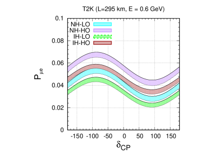
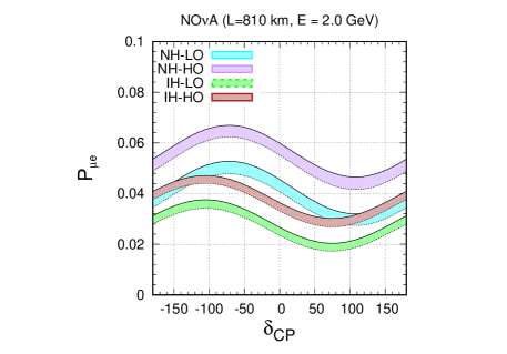
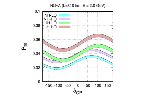
Figure 1: Probability vs $\delta_{CP}~{}$for T2K & NO$\nu$A. The bands are obtained by varying $\theta_{23}$ in lower octant and upper octant. See text for details.

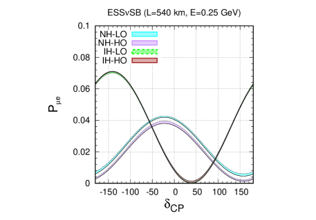
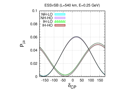
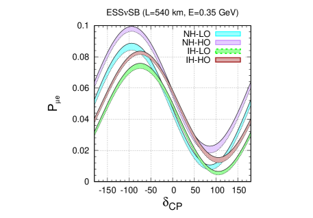
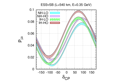
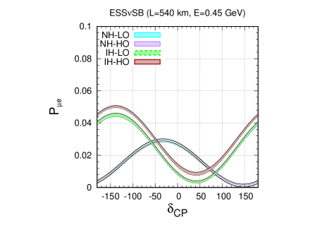
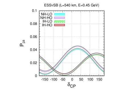
Figure 2: Appearance probability for ESS$\nu$SB for different energies. The bands are obtained by varying $\theta_{23}$ in lower octant and upper octant. See text for details.

In comparison to the LBL experiments the atmospheric neutrinos in ICAL detector can travel through larger baselines and encounter resonance effects. At resonance, the probabilities can be better described by the one mass scale dominance (OMSD) approximation rather than the $\alpha-s_{13}$ approximation in Eq.1. The relevant probabilities $P_{\mu\mu}$ and $P_{\mu e}$ in the OMSD approximation can be expressed as,

$${\mathrm{P^{m}_{\mu e}}}={\mathrm{\sin^{2}\theta_{23}\;\sin^{2}2\theta^{m}_{13}\;\sin^{2}\left[1.27~{}\mathrm{(\Delta m_{31}^{2})^{m}}~{}\frac{L}{E}\right]}}$$ (9)

$${\mathrm{P^{m}_{\mu\mu}}} = {\mathrm{1-\cos^{2}\theta^{m}_{13}\;{\mathrm{\sin^{2}2\theta_{23}}}\;\sin^{2}\left[1.27\;\left(\frac{\mathrm{\Delta m_{31}^{2}}+A+\mathrm{(\Delta m_{31}^{2})^{m}}}{2}\right)\;\frac{L}{E}\right]}}$$ (10)

$$~{}-~{}{\mathrm{\sin^{2}\theta^{m}_{13}\;{\mathrm{\sin^{2}2\theta_{23}}}\;\sin^{2}\left[1.27\;\left(\frac{\mathrm{\Delta m_{31}^{2}}+A-\mathrm{(\Delta m_{31}^{2})^{m}}}{2}\right)\;\frac{L}{E}\right]}}$$

$$~{}-~{}{\mathrm{\sin^{4}\theta_{23}}}\;{\mathrm{\sin^{2}2\theta^{m}_{13}}}\;\sin^{2}\left[1.27\;\mathrm{(\Delta m_{31}^{2})^{m}}\;\frac{L}{E}\right]$$

Due to matter effect the modified mass squared difference ${\mathrm{\mathrm{(\Delta m_{31}^{2})^{m}}}}$ and mixing angle ${\mathrm{\mathrm{\sin^{2}2\theta_{13}^{m}}}}$ are given by ,

$${\mathrm{\mathrm{(\Delta m_{31}^{2})^{m}}}} = {\mathrm{\sqrt{(\mathrm{\Delta m_{31}^{2}}\cos 2\theta_{13}-A)^{2}+(\mathrm{\Delta m_{31}^{2}}\sin 2\theta_{13})^{2}}}}$$

$${\mathrm{\sin 2\theta^{m}_{13}}} = \frac{\mathrm{\mathrm{\Delta m_{31}^{2}}\sin 2\theta_{13}}}{{\mathrm{\sqrt{(\mathrm{\Delta m_{31}^{2}}\cos 2\theta_{13}-A)^{2}+(\mathrm{\Delta m_{31}^{2}}\sin 2\theta_{13})^{2}}}}}$$ (11)

The Mikheyev-Smirnov-Wolfenstein(MSW) matter resonance Wolfenstein (1978); Mikheev and Smirnov (1985, 1986) occurs when,

$$\mathrm{\Delta m_{31}^{2}}\cos 2\theta_{13}=A$$

The MSW resonance happens when $\mathrm{\Delta m_{31}^{2}}>0$ for neutrinos and $\mathrm{\Delta m_{31}^{2}}<0$ for anti-neutrinos. Sine the resonance conditions are opposite for neutrinos and anti-neutrinos therefore the ability to distinguish between neutrinos and anti-neutrinos is crucial for mass hierarchy sensitivity. Hence, the ICAL detector which has charge sensitivity can help unfold the mass hierarchy. The $\sin^{2}\theta_{23}$ term in $P_{\mu e}$ and $\sin^{4}\theta_{23}$ term in $P_{\mu\mu}$ is responsible for the octant sensitivity of ICAL Brahmachari et al. (2003). Detailed discussion on the octant dependence of the probability for atmospheric neutrinos can be found for instance in Chatterjee et al. (2013).

3 Experimental details

In this section we provide a brief description of the experiments used in our study — the currently running long-baseline experiments T2K, NO$\nu$A and also the future proposed long-baseline experiment ESS$\nu$SB along with the atmospheric neutrino experiment ICAL@INO.

T2K (Tokai to Kamioka) Abe et al. (2017) is a 295 km baseline experiment with the flux centered at the neutrino energy around 0.6 GeV generated by JPARC neutrino beam facility at power level higher than 300 kW. T2K has already collected $3.1\times 10^{21}$ protons on target(POT) and is expected to collect a total of $8\times 10^{21}$ in 10 years. So, we have used a total POT of $8\times 10^{21}$ in our simulation. In order to minimize the experimental uncertainty a near and a far detector are used at an angle $2.5^{\circ}$ from the center of the neutrino beam. Using the shape of the $\hat{\rm{C}}$herencov rings, the Super Kamiokande detector (fiducial volume 22.5 kt) for T2K has the ability to distinguish between electron and muon events. In our analysis we have considered 4 years of neutrino and 4 years of anti-neutrino runs for T2K.

NO$\nu$A experiment Adamson et al. (2017) is also a long-baseline neutrino experiment with a baseline of 810 km between the source and the detector. NO$\nu$A uses high intensity 400 kW NuMI beam at Fermi lab. In this experimental set up a relatively smaller, 222 ton near detector and a bigger 15 kiloton far detector are placed at an off axis of $0.8^{\circ}$ from the NuMI beam with peak energy at 2 GeV. In both near and far positions liquid scintillator type detectors are used. NO$\nu$A is currently running at 700 kW beam power corresponding to $7.3\times 10^{20}$ POT yearly and has already collected $8.85\times 10^{20}$ POT. NO$\nu$A is planned to run in 3 years neutrino and 3 years of anti-neutrino mode. In our study we have used the re-optimized NO$\nu$A set up from Agarwalla et al. (2012); Patterson (2012) and have used the full projected run time.

ESS$\nu$SB Baussan et al. (2012, 2014) is a 540 km baseline experiment where high intensity neutrino beam will be produced at the European Spallation Source (ESS) in Lund, Sweden. ESS$\nu$SB Wildner et al. (2016) will focus its research on the second oscillation maximum and plans to use a megaton water $\hat{\rm{C}}$herencov detector. To create a high intensity neutrino beam, they propose to use the linac facility of the European Spallation Source which will produce 2 GeV protons with an average beam power of 5 MW and $27\times 10^{23}$ POT. The ESS$\nu$SB collaboration advocates an optimized set up with 2 years of neutrino and 8 years of anti-neutrino runs Baussan et al. (2014).

$\bf{I}$ndia-based $\bf{N}$eutrino $\bf{O}$bservatory (INO) Ahmed et al. (2017) is a proposal for observing atmospheric neutrinos in a magnetized $\bf{i}$ron $\bf{cal}$orimeter (ICAL) detector. This experiment will look for atmospheric $\nu_{\mu}$ and $\bar{\nu}_{\mu}$ in the GeV energy range. It is proposed to be built in the southern part of India under a mountain with 1 km overall rock coverage. It will house a 50 kt ICAL detector with 1.5 Tesla magnetic field. Because of the magnetic properties of the detector, ICAL can identify the polarity of the charged particles produced by the $\bf{c}$harge $\bf{c}$urrent (CC) interaction of neutrinos with the detector. This gives it the ability to differentiate between neutrinos and anti-neutrinos by identifying the charge of the daughter particles using Resistive Plate Chambers (RPC) as an active detector component.

4 Simulation details

In this section we present the details of our simulation procedure for the LBL experiments T2K, NO$\nu$A and ESS$\nu$SB and the atmospheric neutrino experiment ICAL@INO. We also discuss how the combined analysis of the various experiments are performed.

The simulation for the long-baseline accelerator experiments T2K , NO$\nu$A & ESS$\nu$SB are done using the General Long Baseline Experiment Simulator (GLoBES) package Huber et al. (2005, 2007). In this, the capability of an experiment to determine an oscillation parameter is obtained by a $\chi^{2}$-analysis using frequentist approach. The total $\chi^{2}_{{\rm tot}}$ is composed of $\chi^{2}_{{\rm stat}}$ and $\chi^{2}_{{\rm pull}}$ and is given by the following relation

$$\chi^{2}_{{\rm tot}}=\underset{\xi,\Omega}{\mathrm{min}}\left\{\chi^{2}_{{\rm stat}}(\Omega,\xi)+\chi^{2}_{{\rm pull}}(\xi)\right\}$$ (12)

where $\Omega=\{\theta_{12},\theta_{13},\theta_{23},\Delta m^{2}_{21},\Delta m^{2}_{31},\delta_{CP}\}$ represents the oscillation parameters, $\chi^{2}_{{\rm stat}}$ denotes the poissonian $\chi^{2}$ function and $\chi^{2}_{{\rm pull}}$ consists of the systematic uncertainties incorporated in terms of pull variables $(\xi)$. The “pull" variables considered in our analysis are signal normalization error, background normalization error, energy calibration error on signal & background (tilt). In the “pull" method a penalty term is added in terms of the “pull" variables which is given by $\chi^{2}_{{\rm pulls}}=\sum\limits_{r=1}^{r=4}\xi^{2}_{r}$ in order to account for the systematics errors stated above. The poissonian $\chi^{2}_{{\rm stat}}$ is given by

$$\chi^{2}_{{\rm stat}}(\Omega,\xi)=2\sum\limits_{i}\left\{\tilde{N_{i}}^{{\rm test}}-N_{i}^{{\rm true}}+N_{i}^{{\rm true}}\ln\frac{N_{i}^{{\rm true}}}{\tilde{N_{i}}^{{\rm test}}}\right\}.$$ (13)

The number of events predicted by the theoretical model over a range of oscillation parameters $\Omega$ in the $i^{th}$ bin and is given by

$$\tilde{N_{i}}^{{\rm test}}(\Omega,\xi)=\sum\limits_{k=s,b}{N_{i}}^{k}(\Omega)\left[1+c_{i}^{(k)norm}\xi^{(k)norm}+c_{i}^{(k)tilt}\xi^{(k)tilt}\frac{E_{i}-\bar{E}}{E_{max}-E_{min}}\right]$$ (14)

where, $k=s(b)$ denotes signal(background) and $c_{i}^{norm}$(${c_{i}}^{tilt}$) represents alteration in the number of events by the modification of the “pull" variable $\xi^{norm}$(${\xi}^{tilt}$). $E_{i}$ is the mean reconstructed energy of the $i^{th}$ bin, and $\bar{E}=({E_{max}+E_{min}})/{2}$ is the mean energy over this range with $E_{min}$ and $E_{max}$ denoting the maximum and minimum energy. The systematic errors on the signal and background normalizations are shown in Tab.2 . $N_{i}^{{\rm true}}$ in Eq.13 is given by the sum of simulated signal and background events $N_{i}^{{\rm true}}=N_{i}^{s}+N_{i}^{b}$.
The background channels influencing detection of neutrinos is dependent on the type of detector used. The background channels which contribute for the water $\hat{\rm{C}}$herenkov detectors for T2K and ESS$\nu$SB are the Charged Current(CC) non-Quasielastic(QE) background, intrinsic beam background, neutral current background and mis-identification error. While the main background channels affecting the scintillator detector in NO$\nu$A are CC non-QE, intrinsic beam background, neutral current background. The systematic uncertainties in signal and background normalizations in various channels are summarized in Tab.2. Besides these, the energy calibration errors are also incorporated in the analysis in terms of “tilt" errors. The signal (background) “tilt" errors that have been included are 1%(5%) for T2K, 0.1%(0.1%) for NO$\nu$A and 0.1%(0.1%) for ESS$\nu$SB .

Channel	T2K	NO$\nu$A	ESS$\nu$SB
$\nu_{e}$ appearance	2% (5%)	5% (10%)	5% (10%)
$\bar{\nu}_{e}$ appearance	2% (5%)	5% (10%)	5% (10%)
$\nu_{\mu}$ disappearance	0.1% (0.1%)	2.5% (10%)	5% (10%)
$\bar{\nu}_{\mu}$ disappearance	0.1% (0.1%)	2.5% (10%)	5% (10%)

Table 2: The signal (background) normalization errors for T2K , NO$\nu$A and ESS$\nu$SB .

ICAL is a 50 kt detector which aims to detect $\nu_{\mu}$ and $\bar{\nu}_{\mu}$ along with hadron produced in the detector. Atmospheric flux consist of $\nu_{\mu}$ ($\bar{\nu}_{\mu}$) and $\nu_{e}$($\bar{\nu}_{e}$) both of which will contribute to the number of events observed in the ICAL detector. The events observed in the detector can be expressed as:

$$\frac{d^{2}N}{d\Psi_{\mu}}=(t~{}n_{d})\times\int d\Psi_{\nu}~{}d\Phi_{\mu}~{}\biggl{[}P_{\mu\mu}\frac{d^{3}\Phi_{\mu}}{d\Psi_{\nu}~{}d\Phi_{\nu}}+P_{e\mu}\frac{d^{3}\Phi_{e}}{d\Psi_{\nu}~{}d\Phi_{\nu}}\biggr{]}\frac{d\sigma_{\mu}(E_{\nu})}{d\Psi_{\mu}}$$ (15)

where, $d\Psi_{\alpha}=dE_{\alpha}~{}d\cos\theta_{\alpha}$, $n_{d}$ is the number of nucleon target in the detector, t is the experiment run time, $\Phi_{\mu}$ and $\Phi_{e}$ are the initial flux of muon and electron respectively, $\sigma_{\mu}$ is the differential neutrino interaction cross section. $P_{\mu\mu}$ and $P_{e\mu}$ are the muon survival and appearance probabilities. To reduce the Monte Carlo fluctuations, firstly 1000 years of unoscillated data is generated with Nuance Casper (2002) neutrino generator using Honda neutrino flux and the interaction cross section and the ICAL detector geometry. Each event is then multiplied with the oscillation probability depending on the neutrino energy and path length. Oscillation probability in matter is calculated solving differential neutrino propagation equation in matter using the PREM model for the density profile of the Earth Dziewonski and Anderson (1981). These events are smeared on a bin by bin basis using detector resolutions and efficiencies Chatterjee et al. (2014); Devi et al. (2013) to get realistic simulation of the ICAL detector. Later in our analysis we have scaled down to 10 years of ICAL data. For ICAL@INO both “data" and theory events are simulated in the same way. In our analysis, we have used the resolution and the efficiency obtained for the central part of the ICAL detector Chatterjee et al. (2014) using GEANT4 et al. (2003, 2016, 2006) based simulation for the whole detector. The typical muon energy resolution in the GeV energy range is $\sim 10\%$ and angular resolution is $\sim 1^{\circ}$ and charge identification efficiency is greater than $\sim 95\%$ in the relevant energy rangeThakore et al. (2013). As ICAL has very good energy and angular resolution for the muons produced in the detector, so the events spectrum is categorized in terms of measured muon energy ($E_{\mu}$) and reconstructed muon angle ($\cos\theta_{\mu}$). This binning scheme is referred to as $\bf{2D}$ binning scheme in our analysis. Hadrons are also produced along with muons in the CC interaction with the detector. The hadron resolution is $\sim 85\%$ at $1$ GeV and $\sim 36\%$ at $15$ GeV. It is also possible to extract the hadron energy in event by event basis in CC interaction as $E^{\prime}_{h}=E_{\nu}-E_{\mu}$. Now the inelasticity parameter $y=\frac{E^{\prime}_{h}}{E_{\nu}}$ can be used as an independent parameter with every CC event in the previously mentioned 2D scheme. Analysis with these three independent parameters is referred to as the $\bf{3D}$ binning scheme. Improvement of the sensitivities while using the 3D binning scheme over the 2D scheme has been shown in Devi et al. (2014). The binning scheme is summarized in Tab.3. While generating the data, oscillation parameters are used at their true values whereas the test events are generated using the $3\sigma$ range as mentioned in the Tab.4.

Reconstructed variable	[ Range ] (bin width)	Total bins
	[1 : 4] (0.5)	6
$E^{obs}_{\mu}$ (GeV)	[4 : 7] (1)	3
	[7 : 11] (4)	1
	[-1.0 : -0.4] (0.05)	12
$\cos\theta_{\mu}$	[-0.4 : 0] (0.1)	4
	[0.0 : 1.0] (0.2)	5
	[0.0 : 2.0] (1)	2
$E^{\prime}_{\rm{had}}$ (GeV)	[2.0 : 4.0] (2)	1
	[4.0 : 11.0] (11)	1

Table 3: The binning scheme used in 2D ($E_{\mu}$, $\cos\theta_{\mu}$) and 3D ($E_{\mu}$, $\cos\theta_{\mu}$, $E^{\prime}_{\rm{had}}$) analysis.

As ICAL is not sensitive to $\delta_{CP}~{}$Gandhi et al. (2007), we have not marginalized over test $\delta_{CP}~{}$and fixed the value at $0^{\circ}$ while generating the test events. To get the ICAL@INO sensitivity we perform a $\chi^{2}$ analysis where with $chi^{2}$ defined as:

$$\chi^{2}_{\rm{INO}} = {\stackrel{{\scriptstyle\hbox{min}}}{{\displaystyle\xi_{l}^{\pm}}}}\sum^{N_{E^{obs}_{\mu}}}_{i=1}\sum^{N_{\cos\theta^{obs}_{\mu}}}_{j=1}\sum^{N_{E^{\prime obs}_{had}}}_{k=1}2\left[\left(T^{+}_{ijk}-D^{+}_{ijk}\right)-D^{+}_{ijk}\ln\left(\frac{T^{+}_{ijk}}{D^{+}_{ijk}}\right)\right]+$$ (16)

$$2\left[\left(T^{-}_{ijk}-D^{-}_{ijk}\right)-D^{-}_{ijk}\ln\left(\frac{T^{-}_{ijk}}{D^{-}_{ijk}}\right)\right]+\sum^{5}_{l^{+}=1}\xi^{2}_{l^{+}}+\sum^{5}_{l^{-}=1}\xi^{2}_{l^{-}}~{}.$$

Where $i,j,k$ sums over muon energy, muon angle and hadron energy bins respectively. $T_{ijk},~{}D_{i,j,k}$ refers the predicted (theory) and observed (data) events respectively in $i,j,k$ bin. The $\pm$ sign in theory or observed events refer to the $\mu^{\pm}$ events coming from $\nu^{\pm}_{\mu}$ interactions in the detector. The number of expected events with systematic errors in each bin are given by:

$$T^{+}_{ijk}=T^{0+}_{ijk}\left(1+\sum^{5}_{l^{+}=1}\pi^{l^{+}}_{ijk}\xi_{l^{+}}\right)~{};~{}~{}T^{-}_{ijk}=T^{0-}_{ijk}\left(1+\sum^{5}_{l^{-}=1}\pi^{l^{-}}_{ijk}\xi_{l^{-}}\right)~{}.$$ (17)

where $T^{0\pm}_{ijk}$ refers to the number of theory events without systematic errors in a particular bin $i,j,k$. The systematic uncertainties considered in the analysis using pull method are Gonzalez-Garcia and Maltoni (2004):

• $\pi_{1}=20$% flux normalization error

• $\pi_{2}=10$% cross section error

• $\pi_{3}=5$% tilt error

• $\pi_{4}=5$% zenith angle error

• $\pi_{5}=5$% overall systematics

To incorporate the “tilt" error, the predicted neutrino fluxes is modified using:

$$\Phi_{\delta}(E)=\Phi_{0}(E)\left(\frac{E}{E_{0}}\right)^{\delta}\simeq\Phi_{0}(E)\left(1+\delta\ln\frac{E}{E_{0}}\right),$$ (18)

where, $E_{0}$ is 2 GeV, and $\delta$ is the 1$\sigma$ systematic “tilt" error (5%). Flux uncertainty is included as $\Phi_{\delta}(E)-\Phi_{0}(E)$.

Oscillation parameters	True value	Test range
$\sin^{2}2\theta_{13}$	0.085	fixed
$\sin^{2}\theta_{12}$	0.304	fixed
$\theta_{23}$	$42^{\circ}$ (LO), $48^{\circ}$ (HO)	$39^{\circ}:51^{\circ}$
$\Delta m^{2}_{21}$ (eV2)	$7.4\times 10^{-5}$	fixed
$\Delta m^{2}_{31}$ (eV2)	$2.5\times 10^{-3}$	$(2.35:2.65)\times 10^{-3}$
$\delta_{\rm{CP}}$ (LBL)	$-180^{\circ}:180^{\circ}$	$-180^{\circ}:180^{\circ}$
$\delta_{\rm{CP}}$ (INO)	$-180^{\circ}:180^{\circ}$	$0^{\circ}$(fixed)

Table 4: The true and test values of the oscillation parameters used in our analysis.

For performing the statistical analysis the observed events or data are generated using the true values listed in Tab.4. The predicted or test events are simulated varying the parameters $|\Delta m^{2}_{31}|$, $\sin^{2}\theta_{23}$ in their $3\sigma$ ranges presented in Tab.4. The values of $\theta_{12}$, $\sin^{2}\theta_{13}$ and $\Delta m^{2}_{21}$ are held fixed to their best-fit values while calculating the test events. For LBL experiments $\delta_{CP}~{}$is varied over $0^{\circ}-360^{\circ}$ while generating the test events. For calculating $\chi^{2}$ corresponding to hierarchy or octant sensitivity for a particular experiment marginalization is done over the oscillation parameters which are varied in the 3$\sigma$ range obtained from the global analysis of the current data. If two or more LBL experiments are combined then the $\chi^{2}$ of each experiment are added in the test plane and then the combined $\chi^{2}$ is marginalized over. Since ICAL@INO is insensitive to $\delta_{CP}$, the $\delta_{CP}$(test) is kept fixed for ICAL@INO analysis to save computation time. While calculating the combined $\chi^{2}$ for LBL and ICAL@INO, the marginalization over test-$\delta_{CP}~{}$is first performed for LBL experiments and then the marginalized $\chi^{2}$ is added with the ICAL@INO $\chi^{2}$. This $\chi^{2}$ is further marginalized over the oscillation parameters $|\Delta m^{2}_{31}|$, $\sin^{2}\theta_{23}$ as follows :

$$\chi^{2}_{tot}~{}=~{}\stackrel{{\scriptstyle\hbox{Min}}}{{\hbox{\small{$\theta_{23}$,$|\Delta m^{2}_{31}|$}}}}\biggl{[}\chi^{2}_{INO}+\stackrel{{\scriptstyle\hbox{Min}}}{{\hbox{\small{$\delta_{CP}$}}}}\chi^{2}_{LBL}\biggr{]}.$$ (19)

5 Results and Discussions

5.1 Mass hierarchy sensitivity

The mass hierarchy sensitivity is calculated by taking a true set of parameters assuming NH(IH) as true hierarchy and is compared against the test parameters assuming the opposite hierarchy IH(NH). While calculating the hierarchy sensitivity, marginalization is done over $\theta_{23}$, $|\Delta m^{2}_{31}|$ and $\delta_{CP}~{}$in the range depicted in Tab.4 in the test events (unless otherwise mentioned) while $\theta_{12}$, $\theta_{13}$ and $\Delta m^{2}_{21}$ are kept fixed at their best-fit values.

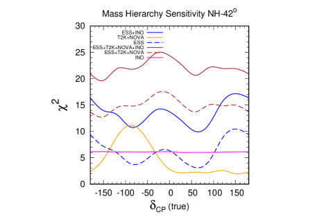
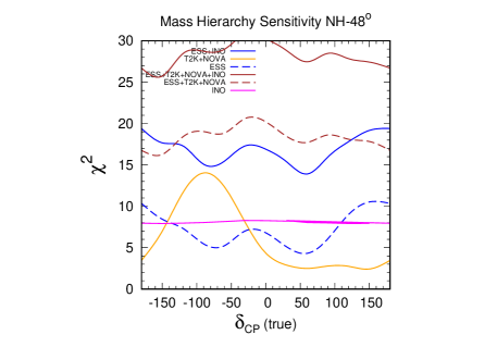
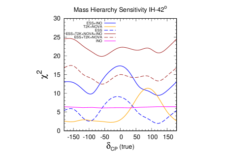
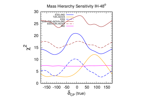
Figure 3: Mass hierarchy sensitivity vs $\delta_{CP}~{}$(true) for ICAL@INO-3D ESS$\nu$SB T2K NO$\nu$A for four hierarchy-octant combinations starting from top right, clockwise in the order NH-LO, NH-HO, IH-HO and IH-LO. Each figure consists of six different experimental combinations which are represented as ICAL@INO (magenta solid curve), ESS$\nu$SB (blue dashed curve), T2K + NO$\nu$A (orange solid curve), ESS$\nu$SB + ICAL@INO (blue solid curve), ESS$\nu$SB + T2K + NO$\nu$A (brown dashed curve) and ESS$\nu$SB + T2K + NO$\nu$A + ICAL@INO (brown solid curve).

In Fig.3 we present the hierarchy sensitivities as a function of true $\delta_{CP}~{}$for the experiments ESS$\nu$SB (2 years neutrino + 8 years anti-neutrino), T2K + NO$\nu$A (3 years neutrino + 3 years anti-neutrino), INO-3D, individually and combined with each other for four hierarchy-octant combinations. These are NH-LO, NH-HO, IH-LO and IH-HO. The representative true values of $\theta_{23}$ for LO and HO are chosen as $42^{\circ}$ and $48^{\circ}$ respectively.

The blue dashed lines in the plots represent the hierarchy sensitivity of ESS$\nu$SB. It is seen that for all the four cases hierarchy sensitivity of ESS$\nu$SB is more for CP conserving values ($0^{\circ}$, $\pm 180^{\circ}$) than for CP violating values ($\pm 90^{\circ}$). Overall, for NH and $\theta_{23}=42^{\circ}$, ESS$\nu$SB can have close to $2\sigma$ hierarchy sensitivity for all values of $\delta_{CP}~{}$reaching upto $3\sigma$ for $\delta_{CP}~{}$= $\pm 180^{\circ}$. The CP dependence of hierarchy sensitivity for NH-HO is similar to that of NH-LO as can be seen from the right panel of the top row. However, the sensitivity is slightly higher because of the higher octant. The panels in the second row show the hierarchy sensitivity for IH-LO and IH-HO. In this case ESS$\nu$SB attains highest hierarchy sensitivity ($\sim 3\sigma$) for $\delta_{CP}~{}$$=0^{\circ}$ but sensitivity is $<2\sigma$ for $\delta_{CP}=\pm 90^{\circ}$.

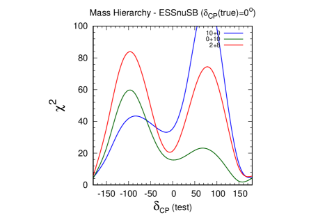
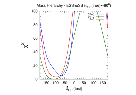
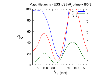
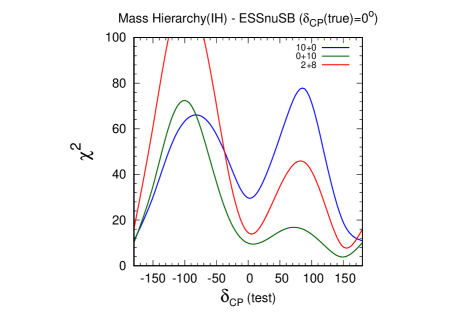
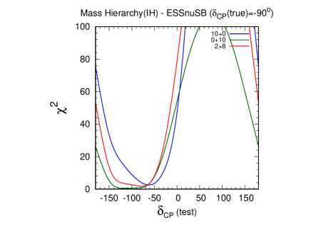
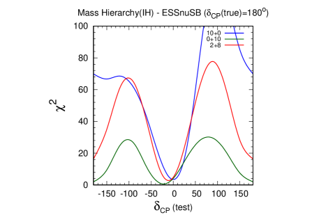
Figure 4: Mass hierarchy sensitivity vs $\delta_{CP}~{}$(test) for ESS$\nu$SB with true $\delta_{CP}~{}$fixed. The top row represents true NH white the bottom row represents true IH. The true octant is fixed as lower octant for all the plots. Each row has plots for three different $\delta_{CP}~{}$(true), which are $0^{\circ}$,$-90^{\circ}$ and $180^{\circ}$ from left to right in the given order. Each figure consists of three different runtime combinations of neutrino and anti-neutrino runs. The blue, green and red curves denote the runtime combinations (in years) of $10\nu+0\bar{\nu}$, $0\nu+10\bar{\nu}$ and $2\nu+8\bar{\nu}$ respectively.

In order to understand the behavior of the hierarchy sensitivity $\chi^{2}$ with $\delta_{CP}~{}$in Fig.4 we plot the hierarchy $\chi^{2}$ as a function of test-$\delta_{CP}~{}$for only neutrino, only anti-neutrino and the mixed runs of 10$\nu$+0$\bar{\nu}$ years, 0$\nu$+10$\bar{\nu}$ years and 2$\nu$+8$\bar{\nu}$ years respectively for the ESS$\nu$SB experiment. One can see that for $\delta_{CP}~{}$= $0^{\circ}$ the minimum for neutrinos come at $\pm 180^{\circ}$ while that of anti-neutrinos occur at $150^{\circ}$. Therefore, the position of the overall minimum combining neutrinos and anti-neutrinos is at $\delta_{CP}~{}$$=\pm 180^{\circ}$. For $\delta_{CP}~{}$(true) $=180^{\circ}$, the neutrino minimum is seen to be at $\delta_{CP}~{}$(test) $=0^{\circ}$ whereas the anti-neutrino minima at $\delta_{CP}~{}$(test) $\approx-30^{\circ}$ and $\pm 180^{\circ}$. The overall minimum of 2$\nu$+8$\bar{\nu}$ years runtime come at $\delta_{CP}~{}$$=-20^{\circ}$. In comparison the figure drawn for true $\delta_{CP}~{}$$=-90^{\circ}$ (the second panel in the first row) shows that the minimum for only neutrino run comes around $-60^{\circ}$ whereas that for only anti-neutrino comes around $-110^{\circ}$. Whereas the combined minimum occurs close to $-90^{\circ}$. Thus for $\delta_{CP}~{}$$=-90^{\circ}$ the wrong hierarchy minima comes at the same CP value as compared to $\delta_{CP}~{}$(true) $=0^{\circ}$, $\pm 180^{\circ}$ where the wrong hierarchy minima are farther from the true value and hence the tension is enhanced. Similar feature is observed in the IH-LO curves (in the lower panel) also. For $\delta_{CP}~{}$(true) $=-90^{\circ}$ the minima for only neutrino, only anti-neutrino and the combined runs occur in the same half plane as $\delta_{CP}~{}$$=-90^{\circ}$ whereas for true $\delta_{CP}~{}$$=0^{\circ}$ the corresponding minima occurs at $\pm 180^{\circ}$ and $150^{\circ}$. Similarly for $\delta_{CP}~{}$$=180^{\circ}$, the minimum for only neutrino run is at $0^{\circ}$, for only anti-neutrino run is at $-30^{\circ}$ and the combined run is close to $-10^{\circ}$. Thus for $\delta_{CP}~{}$$=-90^{\circ}$ the presence of WH-R$\delta_{CP}~{}$degeneracy gives a lower sensitivity as compared to the CP conserving values, where the wrong hierarchy minima come at different wrong CP values for neutrino and anti-neutrino which enhances the tension and hence the $\chi^{2}$. It is seen that the only neutrino run of ESS$\nu$SB can give a better hierarchy sensitivity because of statistics than the combined runs. However, the combined neutrino and anti-neutrino run is expected to give a higher CP sensitivity Baussan et al. (2014).

The magenta curves in Fig.3 represents the hierarchy sensitivity of ICAL@INO. Mass hierarchy sensitivity of ICAL@INO is independent of $\delta_{CP}~{}$because of the sub-dominant effect of $\delta_{CP}~{}$in survival probability and also due to smearing over directions Ghosh et al. (2014a, b). Hence, when ICAL@INO is added to other long-baseline accelerator experiments a constant increase in the sensitivity is observed. This helps to get reasonable sensitivity in the degenerate region. This is reflected by the blue solid curves which demonstrate the hierarchy sensitivity of ESS$\nu$SB + ICAL@INO. Since ICAL@INO has no dependence on $\delta_{CP}~{}$the combined curve follows the ESS$\nu$SB curve. The combination of ESS$\nu$SB + ICAL@INO can give $3\sigma$ hierarchy sensitivity over the whole range of $\delta_{CP}~{}$reaching $4\sigma$ for $\delta_{CP}~{}$= $\pm 180^{\circ}$ for NH-LO. For NH-HO, the combined sensitivity is more than $3.5\sigma$ for all values of $\delta_{CP}~{}$crossing $4\sigma$ for $\pm 180^{\circ}$. For IH-LO, as can be seen from the second row first column of the Fig.3 the combined sensitivity of ESS$\nu$SB + ICAL@INO is more than $\sim 3\sigma$ for all values of $\delta_{CP}~{}$and more than $4\sigma$ for $\delta_{CP}~{}$$=0^{\circ}$. For IH-HO, the sensitivity at $\delta_{CP}~{}$$=0^{\circ}$ can reach $\sim 4.5\sigma$.

The yellow curves in the different panels of Fig.3 represent the hierarchy sensitivity for T2K + NO$\nu$A. We see that for NH-LO/HO highest sensitivity occurs for $\delta_{CP}~{}$$\sim-90^{\circ}$ and the lower half plane (LHP, $-180^{\circ}<$$\delta_{CP}~{}$$<0^{\circ}$) is seen to be favorable for hierarchy. This can be understood from the probability figures for T2K and NO$\nu$A in Fig.1. For instance NH-LO (the cyan band) and $\delta_{CP}~{}$$\sim-90^{\circ}$ does not show any degeneracy for anti-neutrinos. The degeneracy with IH-HO present for neutrinos can be resolved when neutrino and anti-neutrino are combined. Thus the LHP is conducive for hierarchy determination Prakash et al. (2012). For true NH-HO, neutrino has no degeneracy for $\delta_{CP}~{}$= $-90^{\circ}$, whereas the WH-WO-R$\delta_{CP}~{}$degeneracy observed in the anti-neutrino data (purple and green bands in the probability Fig.2 ) can be resolved when combined with neutrino data. Thus the LHP is favorable for hierarchy. For true IH-LO/HO the upper half plane(UHP, $0^{\circ}<$ $\delta_{CP}~{}$$<180^{\circ}$) is favorable for hierarchy, since there is no degeneracy for neutrinos (anti-neutrinos) for $\delta_{CP}~{}$in the UHP.

When T2K + NO$\nu$A $\chi^{2}$ is added to ESS$\nu$SB and marginalized, the CP dependence of the hierarchy sensitivity is governed by all the three experiments. The resultant curve shows highest sensitivity for $\delta_{CP}~{}$$=0^{\circ}$ reaching $4\sigma$ level for both NH-LO and NH-HO. For IH, $4\sigma$ sensitivity is reached for HO for all values of $\delta_{CP}~{}$and for $\delta_{CP}~{}$$=\pm 180^{\circ}$ for LO. Note that the hierarchy sensitivity for ESS$\nu$SB + ICAL@INO for certain values of $\delta_{CP}~{}$could be higher than that of T2K + NO$\nu$A + ESS$\nu$SB.

The brown solid curve represents the combined hierarchy sensitivity of ESS$\nu$SB + T2K + NO$\nu$A + ICAL@INO and it shows sensitivity reach of $\chi^{2}=25$ for all values of $\delta_{CP}~{}$NH-HO. For NH-LO $5\sigma$ sensitivity is reached for $\delta_{CP}~{}$$=0^{\circ}$, while for IH-HO $\delta_{CP}~{}$$=0^{\circ}$, $\pm 180^{\circ}$. For IH-LO, the sensitivity stays slightly higher than $4.4\sigma$ for all values of $\delta_{CP}$. We have also observed a synergy between ICAL@INO and the accelerator based long-baseline experiments owing to $|\Delta m^{2}_{31}|$ tension. This tension happens because atmospheric data slightly prefers lower $|\Delta m^{2}_{31}|$ values while the accelerator data supports the true value.

Note that, the above analyses are done using the $\chi^{2}$ defined in Eq.19 where we have not included any priors. We have also checked the effect of priors over $\delta_{CP}$, $\Delta m^{2}_{31}$ and $\theta_{23}$ taking their $3\sigma$ ranges from the global analysis of the current data. In this case, we obtain up to 9% increment in the sensitivity with prior on $\delta_{CP}$, while priors over $\Delta m^{2}_{31}$ and $\theta_{23}$ does not have any significant effect on the sensitivities. Hence, our results are more conservative.

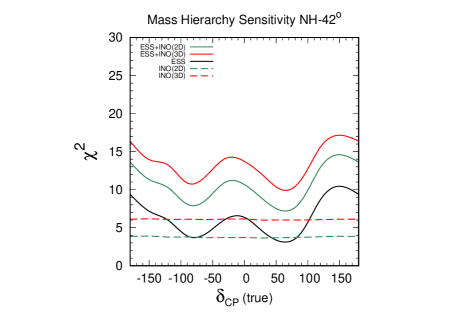
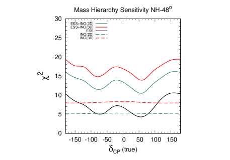
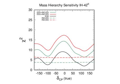
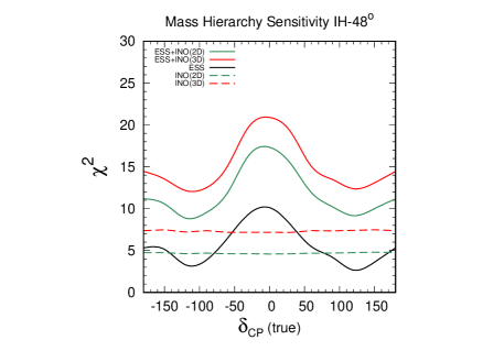
Figure 5: Mass hierarchy sensitivity vs $\delta_{CP}~{}$(true) for ICAL@INO-3D, ICAL@INO-2D and ESS$\nu$SB for four hierarchy-octant combinations starting from top right, clockwise in the order NH-LO, NH-HO, IH-HO and IH-LO. Each figure consists of five different experimental combinations which are represented as ICAL@INO-2D (green dashed curve), ICAL@INO-3D (red dashed curve), ESS$\nu$SB (black solid curve), ESS$\nu$SB + ICAL@INO-2D (green solid curve) and ESS$\nu$SB + ICAL@INO-3D (red solid curve) .

In Fig.5 we compare and quantify the hierarchy sensitivity of ESS$\nu$SB + ICAL@INO for 2D and 3D analysis of the ICAL@INO experiment. The 3D analysis gives better hierarchy sensitivity over 2D because of the inclusion of hadron information in the analysis as described in Sec.3.

5.2 Octant sensitivity

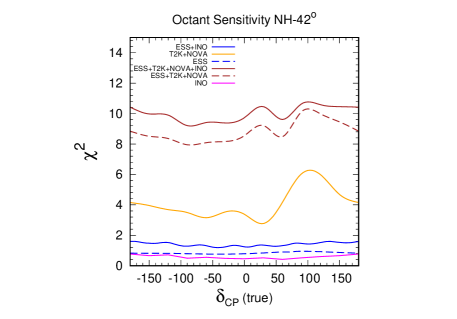
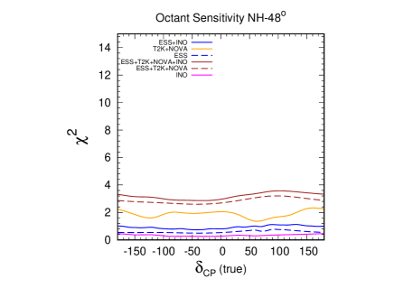
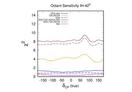
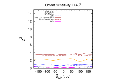
Figure 6: Octant sensitivity vs $\delta_{CP}~{}$(true) for ICAL@INO-3D ESS$\nu$SB T2K NO$\nu$A for four hierarchy-octant combinations starting from top right, clockwise in the order NH-LO, NH-HO, IH-HO and IH-LO. Each figure consists of six different experimental combinations which are represented as ICAL@INO (magenta solid curve), ESS$\nu$SB (blue dashed curve), T2K + NO$\nu$A (orange solid curve), ESS$\nu$SB + ICAL@INO (blue solid curve), ESS$\nu$SB + T2K + NO$\nu$A (brown dashed curve) and ESS$\nu$SB + T2K + NO$\nu$A + ICAL@INO (brown solid curve).

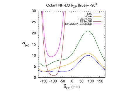
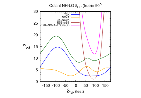
Figure 7: Octant sensitivity vs $\delta_{CP}~{}$(test) for ESS$\nu$SB , T2K and NO$\nu$A with $\delta_{CP}~{}$(true) $=\pm 90^{\circ}$. The true hierarchy and true octant are taken as NH and LO respectively. Left panel represents the octant sensitivities for $\delta_{CP}~{}$(true) $=-90^{\circ}$ and the right panel $\delta_{CP}~{}$(true) $=+90^{\circ}$. Each figure consists of five different experimental combinations which are represented as T2K (blue solid curve), NO$\nu$A (orange solid curve), ESS$\nu$SB (brown solid curve), T2K + NO$\nu$A (green solid curve), ESS$\nu$SB + T2K + NO$\nu$A (magenta solid curve).

To calculate the octant sensitivity we simulate the data for a representative value of true $\theta_{23}$ belonging to LO (HO) and test it by varying $\theta_{23}$ in the opposite octant i.e. HO (LO) along with marginalization over $|\Delta m^{2}_{31}|$, hierarchy and $\delta_{CP}~{}$(for LBL experiments). The plots in Fig.6 show the octant sensitivity for the various experiments. The magenta curves denote the octant sensitivity of ICAL@INO including the hadron information. It is seen that ICAL@INO has very poor octant sensitivity ($\sim<1\sigma$). Although as discussed earlier, the matter effect can break octant degeneracy the sensitivity is low for ICAL@INO, since it can detect only the muon signal. This gets contribution from both $P_{\mu\mu}$ and $P_{e\mu}$ probabilities and the octant sensitivity are opposite which reduces the sensitivity.

T2K, NO$\nu$A and ESS$\nu$SB are accelerator experiments which can detect both the appearance and disappearance channels separately. The blue dashed line denotes the octant sensitivity of ESS$\nu$SB which is again $<1\sigma$ for all the four hierarchy octant combinations. As we have seen from the discussion on probabilities, that ESS$\nu$SB suffers from octant degeneracy over the whole range of $\delta_{CP}~{}$for the E1 and E3 bins. Thus, the octant $\chi^{2}$ gets contribution mainly from the bin E2.

The solid yellow line in Fig.6 represents the combined octant sensitivity for T2K + NO$\nu$A. This combination has $\sim 2\sigma$ octant sensitivity for most of the $\delta_{CP}~{}$range for true NH-LO and IH-LO with peak sensitivity reaching upto $\sim 2.4\sigma$ and $\sim 2.2\sigma$ at $\delta_{CP}~{}$$\sim 90^{\circ}$ respectively. The combination of neutrino and anti-neutrino run help in removing the degenerate wrong octant solutions Ghosh et al. (2016b); Agarwalla et al. (2013); Machado et al. (2014); Coloma et al. (2014). There can also be some synergy between T2K and NO$\nu$A which can enhance octant sensitivity. For instance for true NH-LO, we find a higher sensitivity in the upper half plane of $\delta_{CP}~{}$near $\delta_{CP}~{}$$\sim 100^{\circ}$. This happens because of synergy between T2K and NO$\nu$A. This can be understood from the Fig.7 where we plot the octant sensitivity $\chi^{2}$ vs test-$\delta_{CP}~{}$for T2K, NO$\nu$A and ESS$\nu$SB for NH-LO and two representative values of true $\delta_{CP}~{}$= $\pm 90^{\circ}$. It is seen that for $\delta_{CP}~{}$= $-90^{\circ}$ the minima of NO$\nu$A, T2K and the combined $\chi^{2}$ of NO$\nu$A and T2K, represented by the blue, yellow and the green lines come around $-150^{\circ}$. But for $\delta_{CP}~{}$=$90^{\circ}$ the minimum of T2K comes close to $+90^{\circ}$ but the minimum of NO$\nu$A comes close to $\delta_{CP}~{}$$\sim-20^{\circ}$. The combined minimum comes at $\sim\delta_{CP}=20^{\circ}$ where the T2K and NO$\nu$A contributions are higher than that at their individual minimum. This synergy gives a higher $\chi^{2}$ in the UHP.

For IH-LO (green band in the probability Fig.1), the neutrino probability has no degeneracy for $\delta_{CP}~{}$belonging to the upper half plane. The anti-neutrino probabilities for $\delta_{CP}~{}$in upper half plane has degeneracy with NH-HO at same $\delta_{CP}~{}$(purple band) and IH-HO with $\delta_{CP}~{}$in the lower half plane. But since neutrino events have larger statistics, higher sensitivity is obtained for $\delta_{CP}~{}$in the upper half plane. The $\chi^{2}$ is lower for HO in general. This is because the $\chi^{2}\sim(N_{HO(LO)}-N_{LO(HO)})/N_{HO(LO)}$ for true HO(LO). We see that the numerator is same for both cases whereas the denominator is larger for a true higher octant resulting in a lower sensitivity.

When T2K + NO$\nu$A is combined with ESS$\nu$SB (shown by the dashed brown lines in the Fig.6) an enhancement is observed with the octant sensitivity reaching $\sim 3\sigma$ at $\delta_{CP}~{}$$\sim 90^{\circ}$ for true NH-LO while the octant sensitivity reaches $\sim 2.9\sigma$ for true IH-LO at the same $\delta_{CP}$. But the octant sensitivities are $\sim 1.7\sigma$ for true NH-HO and IH-HO.

It is interesting to understand the enhancement of the octant sensitivity of T2K + NO$\nu$A when combined with ESS$\nu$SB . This synergy can be understood from Fig.7. The brown curve in this figure denotes the octant sensitivity of ESS$\nu$SB as a function of test $\delta_{CP}~{}$while the magenta curve denotes the combined sensitivity of T2K + NO$\nu$A + ESS$\nu$SB . The left panel represents the plots with $\delta_{CP}~{}$(true) = $-90^{\circ}$ while right panel represents $\delta_{CP}~{}$(true) = $90^{\circ}$. Analyzing the first panel i.e. NH-LO and $\delta_{CP}~{}$(true) = $-90^{\circ}$ it is seen that the minima for both T2K and NO$\nu$A come at $\delta_{CP}~{}$(test) = $-150^{\circ}$ hence there is no synergy between T2K and NO$\nu$A as discussed earlier. But, the ESS$\nu$SB minima is at $\delta_{CP}~{}$(test) = $-100^{\circ}$ therefore the overall minima is shifted towards $\delta_{CP}~{}$(test) = $-120^{\circ}$, which gives rise to significant synergy between ESS$\nu$SB and T2K + NO$\nu$A which can be seen from the magenta curve in Fig.7.

The variation in the octant sensitivity $\chi^{2}$ with $\delta_{CP}~{}$(test) is seen to be very rapid for ESS$\nu$SB hence it controls the overall shape of the combined octant sensitivity curve and the position of the minima. As we have discussed earlier, the octant sensitivity for ESS$\nu$SB is contributed by the bin with mean energy 0.35 GeV. As can be seen from Fig.2, the probability for this bin has a sharp variation with $\delta_{CP}$. Thus a slight shift in the $\delta_{CP}~{}$value can cause a large change in the probability and hence in the $\chi^{2}$. Similar feature can also be observed in the second panel for NH-LO and true $\delta_{CP}~{}$= $90^{\circ}$.

Addition of ICAL@INO with T2K + NO$\nu$A + ESS$\nu$SB represented by the solid brown curves, results in slightly higher sensitivity. In this case for true NH-LO $3\sigma$ octant sensitivity is obtained. For true IH-LO the octant sensitivity reaches close to $\sim 3\sigma$ at $\delta_{CP}~{}$$\sim 90^{\circ}$. While for true NH-HO and IH-HO the total sensitivity obtained is close to $2\sigma$. Adding ICAL@INO, results in a constant increase in the $\chi^{2}$, since the ICAL@INO $\chi^{2}$ is almost independent of $\delta_{CP}$.

If we add priors over $\delta_{CP}$, $\Delta m^{2}_{31}$ and $\theta_{23}$ using the $3\sigma$ ranges from the global analysis of the current data we find a 6% increase in octant sensitivity due to the prior on $\delta_{CP}$. But priors over $\Delta m^{2}_{31}$ and $\theta_{23}$ do not play any significant role.

6 Conclusions

The ESS$\nu$SB experiment is planned for discovery of $\delta_{CP}~{}$with a high significance using the second oscillation maximum. In this work, we show how the hierarchy sensitivity of the ESS$\nu$SB experiment can be enhanced by combining with the atmospheric neutrino data at the proposed ICAL detector of the ICAL@INO collaboration as well as the data from the ongoing T2K and NO$\nu$A experiments assuming their full projected runs. We present our results for four true hierarchy - octant combination : NH-LO, NH-HO, IH-LO, IH-HO taking representative values of $\theta_{23}=42^{\circ}$ for LO and $48^{\circ}$ for HO. We find that ESS$\nu$SB has $\sim 2(3)\sigma$ hierarchy sensitivity over the majority of $\delta_{CP}~{}$values for the above hierarchy octant combinations. The mass hierarchy sensitivity of ICAL@INO is independent of $\delta_{CP}~{}$and adding ICAL data to ESS$\nu$SB helps to enhance this to $3(4)\sigma$ depending on hierarchy, octant and $\delta_{CP}~{}$value. Addition of T2K + NO$\nu$A to this combination raises the hierarchy sensitivity farther and $5\sigma$ sensitivity to mass hierarchy can be reached. The overall conservative sensitivities (best sensitivities) for the various hierarchy octant combinations are as follows:

• NH-LO : $\sim$ 4.4(5)$\sigma$

• NH-HO : $\sim$ 5(5.5)$\sigma$

• IH-LO : $\sim$ 4.5(5)$\sigma$

• IH-HO : $\sim$ 4.8(5.3)$\sigma$

We have also explored to what extent the octant sensitivity of ESS$\nu$SB can be improved by combining with ICAL@INO and T2K and NO$\nu$A simulated data. We find that ICAL@INO itself has very low octant sensitivity due to opposite interplay of the survival and appearance channels nullifying the octant sensitivity. However when T2K + NO$\nu$A data is added $2(3)\sigma$ octant sensitivity can be achieved. Additionally, we have shown that despite the poor octant sensitivity of ESS$\nu$SB, it can have interesting synergy with T2K + NO$\nu$A owing to the rapid variation of $P_{\mu e}$ with respect to $\delta_{CP}$ at the second oscillation maximum. Hence, combining ESS$\nu$SB with T2K + NO$\nu$A significantly increases the combined $\chi^{2}$.

In conclusion, our analysis underscores the importance of exploring the synergies between the ongoing experiments T2K and NO$\nu$A and the ESS$\nu$SB experiment and atmospheric neutrino experiment ICAL@INO to give enhanced sensitivity.

References

- Capozzi et al. [2017] F. Capozzi, E. Di Valentino, E. Lisi, A. Marrone, A. Melchiorri, and A. Palazzo, Phys. Rev. D95, 096014 (2017), 1703.04471.
- Esteban et al. [2017] I. Esteban, M. C. Gonzalez-Garcia, M. Maltoni, I. Martinez-Soler, and T. Schwetz, JHEP 01, 087 (2017), 1611.01514.
- de Salas et al. [2018] P. F. de Salas, D. V. Forero, C. A. Ternes, M. Tortola, and J. W. F. Valle, Phys. Lett. B782, 633 (2018), 1708.01186.
- Abe et al. [2014] K. Abe et al. (Hyper-Kamiokande Working Group) (2014), 1412.4673, URL https://inspirehep.net/record/1334360/files/arXiv:1412.4673.pdf.
- Abe et al. [2016] K. Abe et al. (Hyper-Kamiokande proto-) (2016), 1611.06118.
- Acciarri et al. [2015] R. Acciarri et al. (DUNE) (2015), 1512.06148.
- Baussan et al. [2012] E. Baussan, M. Dracos, T. Ekelof, E. F. Martinez, H. Ohman, and N. Vassilopoulos (2012), 1212.5048.
- Baussan et al. [2014] E. Baussan et al. (ESSnuSB), Nucl. Phys. B885, 127 (2014), %****␣ino-lbl-submit-final_jhep_v3.bbl␣Line␣75␣****1309.7022.
- Agarwalla et al. [2014a] S. K. Agarwalla, S. Prakash, and S. Uma Sankar, JHEP 03, 087 (2014a), 1304.3251.
- Ghosh et al. [2016a] M. Ghosh, S. Goswami, and S. K. Raut, Eur. Phys. J. C76, 114 (2016a), 1412.1744.
- Bora et al. [2015] K. Bora, D. Dutta, and P. Ghoshal, Mod. Phys. Lett. A30, 1550066 (2015), 1405.7482.
- Barger et al. [2014] V. Barger, A. Bhattacharya, A. Chatterjee, R. Gandhi, D. Marfatia, and M. Masud, Phys. Rev. D89, 011302 (2014), 1307.2519.
- Deepthi et al. [2015] K. N. Deepthi, C. Soumya, and R. Mohanta, New J. Phys. 17, 023035 (2015), 1409.2343.
- Nath et al. [2016] N. Nath, M. Ghosh, and S. Goswami, Nucl. Phys. B913, 381 (2016), 1511.07496.
- Soumya et al. [2016] C. Soumya, K. N. Deepthi, and R. Mohanta, Adv. High Energy Phys. 2016, 9139402 (2016), 1408.6071.
- Coloma et al. [2013] P. Coloma, P. Huber, J. Kopp, and W. Winter, Phys. Rev. D87, 033004 (2013), 1209.5973.
- Ballett et al. [2017] P. Ballett, S. F. King, S. Pascoli, N. W. Prouse, and T. Wang, Phys. Rev. D96, 033003 (2017), 1612.07275.
- Agarwalla et al. [2017] S. K. Agarwalla, M. Ghosh, and S. K. Raut, JHEP 05, 115 (2017), 1704.06116.
- Ghosh [2016] M. Ghosh, Phys. Rev. D93, 073003 (2016), 1512.02226.
- Ghosh and Yasuda [2017] M. Ghosh and O. Yasuda, Phys. Rev. D96, 013001 (2017), 1702.06482.
- Raut [2017] S. K. Raut, Phys. Rev. D96, 075029 (2017), 1703.07136.
- Das et al. [2018] C. R. Das, J. Pulido, J. Maalampi, and S. Vihonen, Phys. Rev. D97, 035023 (2018), 1708.05182.
- Chakraborty et al. [2018] K. Chakraborty, K. N. Deepthi, and S. Goswami, Nucl. Phys. B937, 303 (2018), 1711.11107.
- Agarwalla et al. [2014b] S. K. Agarwalla, S. Choubey, and S. Prakash, JHEP 12, 020 (2014b), 1406.2219.
- Ahmed et al. [2017] S. Ahmed et al. (ICAL), Pramana 88, 79 (2017), 1505.07380.
- Chatterjee et al. [2013] A. Chatterjee, P. Ghoshal, S. Goswami, and S. K. Raut, JHEP 06, 010 (2013), 1302.1370.
- Akhmedov et al. [2004] E. K. Akhmedov, R. Johansson, M. Lindner, T. Ohlsson, and T. Schwetz, JHEP 04, 078 (2004), hep-ph/0402175.
- Barenboim et al. [2019] G. Barenboim, P. B. Denton, S. J. Parke, and C. A. Ternes, Phys. Lett. B791, 351 (2019), 1902.00517.
- Ghosh et al. [2016b] M. Ghosh, P. Ghoshal, S. Goswami, N. Nath, and S. K. Raut, Phys. Rev. D93, 013013 (2016b), %****␣ino-lbl-submit-final_jhep_v3.bbl␣Line␣250␣****1504.06283.
- Prakash et al. [2014] S. Prakash, U. Rahaman, and S. U. Sankar, JHEP 07, 070 (2014), 1306.4125.
- Agarwalla et al. [2013] S. K. Agarwalla, S. Prakash, and S. U. Sankar, JHEP 07, 131 (2013), 1301.2574.
- Machado et al. [2014] P. A. N. Machado, H. Minakata, H. Nunokawa, and R. Zukanovich Funchal, JHEP 05, 109 (2014), 1307.3248.
- Coloma et al. [2014] P. Coloma, H. Minakata, and S. J. Parke, Phys. Rev. D90, 093003 (2014), 1406.2551.
- Wolfenstein [1978] L. Wolfenstein, Phys. Rev. D17, 2369 (1978).
- Mikheev and Smirnov [1985] S. P. Mikheev and A. Y. Smirnov, Sov. J. Nucl. Phys. 42, 913 (1985).
- Mikheev and Smirnov [1986] S. P. Mikheev and A. Y. Smirnov, Nuovo Cim. C9, 17 (1986).
- Brahmachari et al. [2003] B. Brahmachari, S. Choubey, and P. Roy, Nucl. Phys. B671, 483 (2003), hep-ph/0303078.
- Abe et al. [2017] K. Abe et al. (T2K), Phys. Rev. Lett. 118, 151801 (2017), 1701.00432.
- Adamson et al. [2017] P. Adamson et al. (NOvA), Phys. Rev. Lett. 118, 231801 (2017), 1703.03328.
- Agarwalla et al. [2012] S. K. Agarwalla, S. Prakash, S. K. Raut, and S. U. Sankar, JHEP 12, 075 (2012), 1208.3644.
- Patterson [2012] R. Patterson, Nova collaboration, neutrino 2012 conference, kyoto, japan, (unpublished), http://nova-docdb.fnal.gov/cgi-bin/RetrieveFile?docid=7546&filename=Web_SESSION09_Patterson.pdf&version=2 (2012).
- Wildner et al. [2016] E. Wildner et al., Adv. High Energy Phys. 2016, 8640493 (2016), 1510.00493.
- Huber et al. [2005] P. Huber, M. Lindner, and W. Winter, Comput. Phys. Commun. 167, 195 (2005), hep-ph/0407333.
- Huber et al. [2007] P. Huber, J. Kopp, M. Lindner, M. Rolinec, and W. Winter, Comput. Phys. Commun. 177, 432 (2007), hep-ph/0701187.
- and [2008] I. K. and, Journal of Physics: Conference Series 136, 022018 (2008), URL https://doi.org/10.1088%2F1742-6596%2F136%2F2%2F022018.
- Casper [2002] D. Casper, Nucl. Phys. Proc. Suppl. 112, 161 (2002), [,161(2002)], hep-ph/0208030.
- Dziewonski and Anderson [1981] A. M. Dziewonski and D. L. Anderson, Phys. Earth Planet. Interiors 25, 297 (1981).
- Chatterjee et al. [2014] A. Chatterjee, K. K. Meghna, K. Rawat, T. Thakore, V. Bhatnagar, R. Gandhi, D. Indumathi, N. K. Mondal, and N. Sinha, JINST 9, P07001 (2014), 1405.7243.
- Devi et al. [2013] M. M. Devi, A. Ghosh, D. Kaur, L. S. Mohan, S. Choubey, A. Dighe, D. Indumathi, S. Kumar, M. V. N. Murthy, and M. Naimuddin, JINST 8, P11003 (2013), 1304.5115.
- et al. [2003] S. A. et al., Nuclear Instruments and Methods in Physics Research Section A: Accelerators, Spectrometers, Detectors and Associated Equipment 506, 250 (2003), ISSN 0168-9002, URL http://www.sciencedirect.com/science/article/pii/S0168900203013688.
- et al. [2016] J. A. et al., Nuclear Instruments and Methods in Physics Research Section A: Accelerators, Spectrometers, Detectors and Associated Equipment 835, 186 (2016), ISSN 0168-9002, URL http://www.sciencedirect.com/science/article/pii/S0168900216306957.
- et al. [2006] J. A. et al., IEEE Transactions on Nuclear Science 53, 270 (2006), ISSN 0018-9499.
- Thakore et al. [2013] T. Thakore, A. Ghosh, S. Choubey, and A. Dighe, JHEP 05, 058 (2013), 1303.2534.
- Devi et al. [2014] M. M. Devi, T. Thakore, S. K. Agarwalla, and A. Dighe, JHEP 10, 189 (2014), 1406.3689.
- Gandhi et al. [2007] R. Gandhi, P. Ghoshal, S. Goswami, P. Mehta, S. U. Sankar, and S. Shalgar, Phys. Rev. D76, 073012 (2007), 0707.1723.
- Gonzalez-Garcia and Maltoni [2004] M. C. Gonzalez-Garcia and M. Maltoni, Phys. Rev. D 70, 033010 (2004), URL https://link.aps.org/doi/10.1103/PhysRevD.70.033010.
- Ghosh et al. [2014a] M. Ghosh, P. Ghoshal, S. Goswami, and S. K. Raut, Phys. Rev. D89, 011301 (2014a), 1306.2500.
- Ghosh et al. [2014b] M. Ghosh, P. Ghoshal, S. Goswami, and S. K. Raut, Nucl. Phys. B884, 274 (2014b), 1401.7243.
- Prakash et al. [2012] S. Prakash, S. K. Raut, and S. U. Sankar, Phys. Rev. D86, 033012 (2012), 1201.6485.