Sensitivities and synergies of DUNE and T2HK

Abstract

Long-baseline neutrino oscillation experiments, in particular Deep Underground Neutrino Experiment (DUNE) and Tokai to Hyper-Kamiokande (T2HK), will lead the effort in the precision determination of the as yet unknown parameters of the leptonic mixing matrix. In this article, we revisit the potential of DUNE, T2HK and their combination in light of the most recent experimental information. As well as addressing more conventional questions, we pay particular attention to the attainable precision on $\delta$, which is playing an increasingly important role in the physics case of the long-baseline programme. We analyse the complementarity of the two designs, identify the benefit of a programme comprising distinct experiments and consider how best to optimise the global oscillation programme. This latter question is particularly pertinent in light of a number of alternative design options which have recently been mooted: a Korean second detector for T2HK and different beams options at DUNE. We study the impact of these options and quantify the synergies between alternative proposals, identifying the best means of furthering our knowledge of the fundamental physics of neutrino oscillation.

1 Introduction

Our knowledge of the neutrino sector has undergone a sea-change over the last decade. The oscillation mechanism has been well established as the explanation of the anomalous solar and atmospheric neutrino flavour ratios, and the paradigm has been subjected to scrutiny from long-baseline accelerator and reactor experiments resulting in a measurement of the final mixing angle $\theta_{13}$ [1, 2, 3, 4]. Although some short-baseline anomalies still remain unexplained [5, 6, 7], the oscillation mechanism has leapt many hurdles to become a part of the new Standard Model (SM). However, some significant unknowns remain: the ordering of neutrino masses parameterized by the sign of $\Delta m^{2}_{31}$, the existence and extent of CP violation (CPV) or maximal CP violation in leptonic mixing, and the precise value, including crucially the octant, of $\theta_{23}$. In addition, the current precision on the oscillation parameters is insufficient to rule out many theoretical models, for example those discussed recently in Refs. [8, 9, 10, 11]. These models can offer predictions for $\delta$ — potentially explaining maximally CP violating or CP conserving values — as well as the octant, and the mass ordering.

With the intention of building on the progress of the oscillation programme, the international community has conceived a range of future facilities with the potential to explore the final unknowns in the conventional oscillation paradigm, and to hunt for tensions in the data which might indicate that a richer extension of the SM is required. There are three major strands in the future experimental neutrino oscillation programme: short-baseline experiments such as those comprising the SBN programme [12], intermediate baseline reactor facilities, RENO-50 and JUNO [13, 14, 15], and long-baseline experiments (LBL) such as LBNF-DUNE and T2HK [16, 17, 18, 19, 20, 21]. In this article we focus on these latter two proposals for novel long-baseline facilities: Long-Baseline Neutrino Facility-Deep Underground Neutrino Experiment (LBNF-DUNE, referred to subsequently as DUNE) and Tokai to Hyper-Kamiokande (T2HK). DUNE is the flag-ship long baseline experiment of the Fermilab neutrino programme [20, 21]. It consists of a new beam sourced at Fermilab and a detector complex at Sanford Underground Research Facility (SURF) in South Dakota separated by a distance of 1300 km. Over this distance, neutrinos produced in the decays of secondary particles from proton collisions at Fermilab will propagate, undergoing oscillations and scattering processes in the matter of the Earth. The appreciable matter effects will modify the probability of detecting a given flavour of neutrino, in a way that will ultimately make the facility highly sensitive to the mass ordering while the broad spectrum of events arising from its on-axis flux also allows for significant sensitivity to the unknown CPV phase $\delta$. The detector will use Liquid Argon Time Projection Chamber (LAr-TPC) technology, allowing for strong event reconstruction. As a result, a high signal to background ratio is expected. T2HK [19] in contrast was conceived with a smaller baseline of 295 km and a different detector technology. Building on the successes of Kamiokande and Super-Kamiokande [22], Hyper-Kamiokande will employ Water Čerenkov technology at a significantly larger scale, with fiducial volumes on the order of hundreds of kilotonnes. Matter effects for this facility will be smaller due to the shorter baseline (although non-negligible), and the significantly enhanced event rate will allow for a high-statistics comparison between neutrino and anti-neutrino modes, searching for fundamental asymmetries due to the CP violating phase $\delta$.

Much work has been done over the years assessing the physics reach of T2HK [19, 23, 24] and DUNE [25, 21, 26, 27, 28] (along with its predecessor designs LBNE [20, 29, 30, 31, 24] and LBNO [32, 33, 24]). In this article, we revisit the physics sensitivity of DUNE and T2HK for key measurements relating to the mass ordering, $\delta$ phase and the mixing angle $\theta_{23}$, focusing in particular on the combined reach of these designs. Recently, as the designs for T2HK and DUNE have matured, both collaborations have considered significant alterations to the benchmark proposals in Refs. [19] and [25, 21]. The nuPIL (neutrinos from a PIon beam Line) design [34, 35, 36], developed at Fermilab, is a novel beam technology building on accelerator R&D work done for the neutrino factory [37]. Although nuPIL is no longer in consideration by the DUNE collaboration, its unique design leads to phenomenology which may be of interest to future work. nuPIL foresees the collection and sign selection of pions from a conventional beam, which are directed though a beam line and decay to produce neutrinos. This selection and manipulation of the secondary beam forces unwanted parent particles out of the beam resulting in a particularly clean flux. This screening process presents a particular advantage over conventional neutrino beams, where the contamination of the flux due to mesons of the wrong sign can limit the sensitivity of the antineutrino channel. In the latter case, the contamination from intrinsic $\nu_{\mu}$ is effectively enhanced by the cross-section differences. This increases the relative number of wrong-sign events, and reduces the signal over background ratio. The simulated flux is also notably narrower than the DUNE reference design (although this could be changed through modification of the design) which will alter the sensitivity to the oscillation probability. In a parallel development, T2HK has reconsidered the location of its second detector module. The current design divides the detector into two modules installed at Kamioka following a staged implementation [38]: an initial data-taking period would use a single tank during which the second tank would be constructed and would start taking data after $6$ years to further boost the statistical power of the experiment. Instead of this plan, the suggestion has been made to locate the second tank in South Korea at a baseline distance of between $1000$ – $1300$ km from J-PARC [39, 40, 41, 42, 43]. This would allow T2HK + Korea (T2HKK) to collect data from two different baselines and with two different off-axis angles (and consequently energy spectra), crucially altering the phenomenology of the experiment.

Although the question of the combined sensitivity of DUNE and T2HK has been studied before (most recently in [44]), our work brings three new elements to the discussion. Firstly, our work incorporates the significant redesign and development work that has been performed in the last few years on both designs. Our simulation of T2HK is particularly noteworthy, departing significantly from those used in previous comparable analyses [44] by incorporating up-to-date information about detector performance from the collaboration’s in-house simulation, and has been carefully calibrated against previously published results. Secondly, we thoroughly address the precision measurement of $\delta$ and its phenomenology, often deemed a secondary question in earlier studies, but one which is increasingly central to the aims of the long-baseline programme, and which has significant theoretical implications. Finally, we provide a detailed discussion of the differences between the two designs as well as their potential redesigns (nuPIL, T2HKK) and a quantification of their complementarity in an attempt to identify the optimal choice from a global perspective.

We start our discussion with a brief recap of the relevant phenomenology of oscillation physics in Section 2. In Section 3, we describe the details of DUNE and T2HK (including their alternative designs) taken into account in our simulations. Section 4 is devoted to the results of our simulations assuming the standard configurations of each experiment which look at mass ordering sensitivity, CP violation discovery, the ability to exclude maximally CP violating values of $\delta$, the expected precision on $\theta_{23}$ and the ability to resolve the octant. We present an analysis of the complementarity for precision on $\delta$ in Section 5, taking care to discuss the interplay of factors which influence this measurement. In Section 6, we reconsider these physics goals in light of the alternative deigns for DUNE and T2HK. We end our study with some concluding remarks in Section 7.

2 Oscillation phenomenology at DUNE and T2HK

The fundamental parameters which describe the oscillation phenomenon are the angles and Dirac phase of the Pontecorvo-Maki-Nakagawa-Sakata (PMNS) mixing matrix as well as two independent mass-squared splittings, e.g. $\Delta m^{2}_{21}$ and $\Delta m^{2}_{31}$. The PMNS matrix is the mapping between the bases of mass and flavour states (denoted with Latin and Greek indices, respectively), which can be written as

$$\nu_{\alpha}=U_{\alpha i}^{*}\nu_{i},$$

where $U$ will be expressed by the conventional factorization [45]:

$$U_{\mathrm{PMNS}} =U_{23}U_{13}U_{12}P,$$

$$=\left(\begin{matrix}1&0&0\\ 0&c_{23}&s_{23}\\ 0&-s_{23}&c_{23}\end{matrix}\right)\left(\begin{matrix}c_{13}&0&s_{13}e^{-\mathrm{i}\delta}\\ 0&1&0\\ -s_{13}e^{\mathrm{i}\delta}&0&c_{13}\end{matrix}\right)\left(\begin{matrix}c_{12}&s_{12}&0\\ -s_{12}&c_{12}&0\\ 0&0&1\end{matrix}\right)\left(\begin{matrix}e^{\mathrm{i}\alpha_{1}}&0&0\\ 0&e^{\mathrm{i}\alpha_{2}}&0\\ 0&0&1\end{matrix}\right),$$

$$=\left(\begin{matrix}c_{12}c_{13}&s_{12}c_{13}&s_{13}e^{-\mathrm{i}\delta}\\ -s_{12}c_{23}-c_{12}s_{23}s_{13}e^{\mathrm{i}\delta}&c_{12}c_{23}-s_{12}s_{23}s_{13}e^{\mathrm{i}\delta}&s_{23}c_{13}\\ s_{12}s_{23}-c_{12}c_{23}s_{13}e^{\mathrm{i}\delta}&-c_{12}s_{23}-s_{12}c_{23}s_{13}e^{\mathrm{i}\delta}&c_{23}c_{13}\end{matrix}\right)P,$$

where $P$ is a diagonal matrix containing two Majorana phases $\alpha_{1}$ and $\alpha_{2}$ which play no role in oscillation physics. The mixing angles $\theta_{12}$, $\theta_{13}$ and $\theta_{23}$ are often referred to as the solar, reactor and atmospheric mixing angles respectively; all of these angles are now known to be non-zero [46]. The remaining parameter in $U$ is the phase $\delta$, which is currently poorly constrained by data. This parameter dictates the size of CP violating effects in vacuum during oscillation. All such effects will be proportional to the Jarlskog invariant of $U_{\text{PMNS}}$,

$$J=\frac{1}{8}\sin\delta\sin\left(2\theta_{23}\right)\sin\left(2\theta_{13}\right)\sin\left(2\theta_{12}\right)\cos\theta_{13}.$$

For the theory to manifest CP violating effects, $J$ must be non-zero. Given our knowledge of the mixing angles, the exclusion of $\delta\notin\{0,\pi\}$ would be sufficient to establish fundamental leptonic CP violation.

Long-baseline experiments such as DUNE and T2HK aim to improve our knowledge of $U$, as well as the atmospheric mass-squared splitting, by the precision measurement of both the appearance $\nu_{\mu}\to\nu_{e}$ and disappearance oscillation channels $\nu_{\mu}\to\nu_{\mu}$, as well as their CP conjugates. In the following section, we will discuss the key aims of the long-baseline program and the important design features of these experiments which lead to their sensitivities. To facilitate this discussion, we introduce an approximation of the appearance channel probability following Ref. [47], which is derived by performing a perturbative expansion in the small parameter $\epsilon\equiv\Delta m^{2}_{21}/\Delta m^{2}_{31}\approx 0.03$ under the assumption that $\sin^{2}\theta_{13}=\mathcal{O}(\epsilon)$. The expression for the oscillation probability is decomposed into terms of increasing power of $\epsilon$,

$$P(\nu_{\mu}\to\nu_{e};E,L)\equiv P_{1}+P_{\frac{3}{2}}+\mathcal{O}\left(\epsilon^{2}\right),$$ (2.1)

where $E$ is the neutrino energy, $L$ the oscillation baseline, and the ordered terms $P_{n}=\mathcal{O}(\epsilon^{n})$ are given by

$$P_{1} =\frac{4}{(1-r_{A})^{2}}\sin^{2}\theta_{23}\sin^{2}\theta_{13}\sin^{2}\left(\frac{(1-r_{A})\Delta L}{2}\right),$$ (2.2)

$$P_{\frac{3}{2}} =8J_{r}\frac{\epsilon}{r_{A}(1-r_{A})}\cos\left(\delta+\frac{\Delta L}{2}\right)\sin\left(\frac{r_{A}\Delta L}{2}\right)\sin\left(\frac{(1-r_{A})\Delta L}{2}\right),$$ (2.3)

where $J_{r}=\cos\theta_{12}\sin\theta_{12}\cos\theta_{23}\sin\theta_{23}\sin\theta_{13}$, $r_{A}=2\sqrt{2}G_{\text{F}}N_{e}E/\Delta m^{2}_{31}$, with $N_{e}$ denoting the electron density in the medium, and $\Delta=\Delta m^{2}_{31}/2E$. Using the same scheme, the disappearance channel can be written at leading order as

$$P(\nu_{\mu}\to\nu_{\mu};E,L)=1-\sin^{2}(2\theta_{23})\sin^{2}\left(\frac{\Delta L}{2}\right)+\mathcal{O}(\epsilon).$$ (2.4)

For both channels, equivalent expressions for antineutrino probabilities can be obtained by the mapping $r_{A}\to-r_{A}$ and $\delta\to-\delta$.

2.1 Mass ordering, CPV and the octant of $\theta_{23}$

The sensitivity of long-baseline experiments to the questions of the neutrino mass ordering, the existence of CPV and the octant of $\theta_{23}$, are by now well studied topics (for a recent review see e.g. Ref. [52]). To help us clarify the role of the designs of DUNE and T2HK, as well as their possible modifications, we will briefly recap how experiments on these scales derive their sensitivities using the approximate formulae expressed by Eqs. (2.2), (2.3) and (2.4).

The dependence on the sign of $\Delta m^{2}_{31}$, and therefore the mass ordering, arises at long-baselines from the interplay with matter, where forward elastic scattering can significantly enhance or suppress the oscillation probability. This is governed by the parameter $r_{A}$ in Eq. (2.1) and goes to zero in the absence of matter. Changing from Normal Ordering (NO, $\Delta m^{2}_{31}>0$) to Inverted Ordering (IO, $\Delta m^{2}_{31}<0$) requires the replacements $\Delta\to-\Delta$ and $r_{A}\to-r_{A}$. However, in vacuum ($r_{A}=0$) the leading-order term in Eq. (2.1) remains invariant under this mapping. This invariance is broken once a matter term is included ($r_{A}\neq 0$), and the oscillation probability acquires a measurable enhancement or suppression dependent on the sign of $\Delta m^{2}_{31}$. The size of this enhancement increases with baseline length, and this effect is expected to be very relevant for appearance channels at a long-baseline experiment $\nu_{\mu}\rightarrow\nu_{e}$ and $\bar{\nu}_{\mu}\rightarrow\bar{\nu}_{e}$. However, the determination of the mass ordering is further facilitated by the contrasting behaviour of neutrinos and antineutrinos. Due to the dependence on $r_{A}$, for NO larger values of the matter density cause an enhancement and a shift in the probability for $\nu_{\mu}\to\nu_{e}$ oscillation at the first maximum, whilst suppressing the probability for $\overline{\nu}_{\mu}\to\overline{\nu}_{e}$. This behaviour is reversed for IO, with neutrinos seeing a suppression and antineutrinos, an enhancement. Moreover, matter effects also affect the energies of the first oscillation maxima for neutrinos and antineutrinos. Through precise measurements around the first maxima, these shifts can be observed allowing long-baseline oscillation experiments to determine the mass ordering.

To detect CPV in neutrino oscillation an experiment requires sensitivity to $\delta$. Unfortunately, the leading order appearance probability $P_{1}$ is independent of the CP phase $\delta$ in vacuum, as seen in Eq. (2.2). CP asymmetries between neutrino and antineutrino channels first appear with the subdominant term $P_{\frac{3}{2}}$. In the presence of a background medium, CP violating effects are instead introduced in $P_{1}$ due to $r_{A}$ which differs by a sign for neutrinos and antineutrinos; however, these offer no sensitivity to the fundamental CP violating parameter $\delta$. As the sensitivity to $\delta$ is subdominant and masked by CP asymmetry arising from matter effects, extracting the CP phase is a more challenging measurement, requiring greater experimental sensitivity. Long baseline (LBL) experiments can obtain sensitivity to $\delta$ by looking not only at the first maximum but also at the spectral differences between CP conjugate channels. In particular, an important role is played by low-energy events in the sensitive determination of $\delta$ [31, 53, 54, 55]: around the second maximum, CP dependent terms of the oscillation probability are more significant. Although accessing these events can be a challenging experimental problem, and low statistics or large backgrounds could limit their potential [53], their benefit is clear from recent experimental work [56].

The atmospheric mixing angle is known to be large and close to maximal $\theta_{23}\approx\pi/4$, but it is not currently established if it lies in the first octant $\theta_{23}<\pi/4$ or the second octant $\theta_{23}>\pi/4$. We see in Eq. (2.2) that the appearance channel is sensitive to the octant. However, we also see that changing the octant enhances or suppresses the first maximum of the appearance channel in much the same way as the matter enhancement. For this reason, the sensitivity to these questions can be expected to be correlated; however, this correlation will be reduced when data from both neutrino and antineutrino is available as this effect is the same in both CP conjugate channels. The determination of $\theta_{23}$ is also known to be beset by issues of degeneracy with $\delta$ which can complicate its determination [57, 58, 52]. As both of these parameters enter the second-order terms in Eq. (2.2), the freedom to vary $\delta$ can be used to mask the effects of a wrong octant, making their joint determination more challenging. Fortunately, a precise measurement of $\sin(2\theta_{23})$ is possible through the disappearance channel, helping to break this degeneracy. Also, spectral information is expected to mitigate this problem.

2.2 Precision on $\delta$

Although the question of the existence of leptonic CP violation often dominates discussions about $\delta$, the precision measurement of $\delta$ could prove to be the most valuable contribution of the long-baseline programme. To determine the existence of fundamental leptonic CP violation it suffices to exclude the CP conserving values $\delta=0$ and $\delta=\pi$, those values corresponding to a vanishing Jarlskog invariant. Therefore the discovery potential of a facility to CP violation is fundamentally linked to the precision attainable for measurements of $\delta$ in the neighbourhood of $0$ and $\pi$. However, the question of precision on $\delta$ goes beyond CP violation discovery. Many models of flavour symmetries, for example, are consistent with the known oscillation data and make predictions for $\delta$. No experiment on comparable time-scales is expected to be able to compete with precision measurements of $\delta$ from DUNE and T2HK.

It can be shown that the precision expected on $\delta$ worsens significantly around $\delta=\pm\frac{\pi}{2}$, and that this is because of the probability itself [66]. Looking at the CP sensitive term in Eq. (2.3) at energies around the first maximum, where $\Delta L/2\approx\pi/2$, we can approximate the probability by

$$P_{\frac{3}{2}}\approx-8J_{r}\frac{\epsilon}{r_{A}(1-r_{A})}\sin\delta\sin\left(\frac{r_{A}\Delta L}{2}\right)\sin\left(\frac{(1-r_{A})\Delta L}{2}\right).$$

The highest sensitivity to $\delta$ is found when this function is most sensitive to changes in $\delta$, information naturally encoded in the function’s first derivative. Due to the sinusoidal nature of the function, when the CP term has its largest effect ($|\sin\delta|=1$), it is at a maximum and consequently its gradient is at a minimum. Therefore, we expect the errors on $\delta$ to be small around $0$ and $\pi$, when even though the absolute size of the CP sensitive terms are small, they are most sensitive to parameter shifts. Taking matter into account moves the location of the worst sensitivity away from $\delta=\pm\frac{\pi}{2}$. Assuming we are close to the first maximum, and introducing a dimensionless parameter $\xi$ to describe the deviation from this point (where $\xi=0$ corresponds to the first maximum), the relevant parameter governing the phase of the sinusoidal terms can be expressed by

$$\Delta L=\pi\frac{1+\xi}{1-r_{A}},$$ (2.5)

we can find the value of $\delta$ for which we expect the worst sensitivity by minimising the gradient of Eq. (2.3), which occurs for the values

$$\delta\approx-\frac{\pi}{2}\frac{1+\xi}{1-r_{A}}+\pi n,$$ (2.6)

for $n\in\mathbb{Z}$. From this formula it is clear that the value of $\delta$ with the worst sensitivity shifts away from $\frac{(2n+1)\pi}{2}$ in a direction governed by the signs of $r_{A}$ and $\xi$. Specifically, the dependence on $r_{A}$ means that the neutrino and anti-neutrino mode sensitivities at fixed energy have their worst sensitivity for different true values of $\delta$. Running both CP conjugate channels in a single experiment allows each channel to compensate for the poorer performance of the other at certain values of $\delta$, helping to smooth out the expected precision [66]. In this way, the multichannel nature of LBL experiments allows for a greater physics reach than a single channel experiment.

The argument above assumed that all events came from a fixed energy defined implicitly by $\xi$ in Eq. (2.5). Due to the dependence on $\xi$ in Eq. (2.6), having information from different energies will also be complementary, acting analogously to the combination of neutrino and antineutrino data by mitigating the poorest performance. Although all LBL experiments aim to include the first maximum, where event rates are highest, none have a purely monochromatic beam and so-called wide-band beams include considerable information from other energies. Therefore such experiments can be expected to avoid the significant loss of sensitivity predicted by the simple analytic formula. We can infer, however, that a narrow beam focused on the first maximum in the presence of small matter effects should have a worse sensitivity at maximal values of $\delta$ compared to CP conserving values [66].

With reference to the traditional designs of T2HK and DUNE, from the above discussion we can infer that T2HK can be expected to have a greater range of expected precisions as we vary $\delta$ than DUNE. In particular, due to its narrower beam and small matter effects, we expect markedly poorer performance for T2HK at $\delta\in\{-\frac{\pi}{2},\frac{\pi}{2}\}$. DUNE on the other hand will be less variable as its broad band mitigates the total loss of sensitivity at certain energies, and its large matter effect helps to stabilise performance, but it can be expected to see its worst sensitivity at values of $\delta$ slightly displaced from $0$ and $\pi$, where the sensitivity at the first maximum is worst. This suggests a degree of complementarity of the wide-band and narrow-band beams when it comes to precision measurements of $\delta$: a narrow-band focused on the first maximum is optimal for precision around $0$ and $\pi$ (and by implication, for CPV discovery) while a wide-band beam should perform better for precision measurements around $\delta=\pm\frac{\pi}{2}$. This general behaviour will be relevant not only for the traditional designs of DUNE and T2HK, but also their possible redesigns: nuPIL could lead to a narrowing of the neutrino flux, and T2HKK could see a wider-band component in its flux, or a narrow-band component focused away from the first maximum. The interplay of these factors will be explored in more detail in Section 5.

3 Simulation details

To better understand the sensitivities and complementarity of DUNE and T2HK (including their potential redesigns), we have performed a simulation of the experiments in isolation and in combination. We are using the General Long Baseline Experiment Simulator (GLoBES) libraries [67, 68] and in the following sections, we will describe the features of our modelling of the two facilities and the statistical treatment.

3.1 DUNE

The DUNE experiment consists of a new neutrino source, known as Long Baseline Neutrino Facility (LBNF), a near detector based at Fermilab and a LArTPC detector complex located in SURF a distance of 1300 km away. Several variants of the LBNF beam have been developed. In this work, we study three neutrino fluxes: a 2-horn optimised beam design [21, 69], a 3-horn optimised beam design [70, 71], and the neutrinos from a PIon beam Line (nuPIL) [34, 35, 36, 72]. We show all three fluxes used in our simulations in Fig. 1.

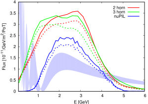
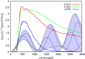
Figure 1: Left: $\nu_{\mu}$ ($\overline{\nu}_{\mu}$) flux component in $\nu$-mode ($\bar{\nu}$-mode) shown as solid (dashed) lines for 2-horn optimised, 3-horn optimised, and nuPIL beam designs. Right: the fluxes for $\nu$-mode shown as a function of $L/E$. In both panels, the shaded region shows the envelope of the oscillation probability as $\delta$ is varied over its full range. The black lines in the right panel show the probability for $\delta\in\{0,\frac{\pi}{2},\pi,\frac{3\pi}{2}\}$.

The 2-horn optimised beam has been designed to maximise the sensitivity to CP violation [21]. In our simulation, we take the proton energy to be $80$ GeV, and follow a staged implementation of the beam power in line with the DUNE proposal, which assumes the beam power will double after 6 years [73]. Our simulation assumes a power of $1.07$ MW and $1.47\times 10^{21}$ protons on target (POT) per year for the first 6 years, and $2.14$ MW ($2.94\times 10^{21}$ POT per year) afterwards. Thanks to constant development work by the DUNE collaboration, an additional optimised beam has also been designed. This 3-horn design has a stronger focus on producing lower energy events, leading to an increase in flux between $0.5$ GeV and $1.5$ GeV. This leads to a greater number of expected events from around the second oscillation maximum, which is well-known to be particularly sensitive to the phase $\delta$. For this design, the proton energy is assumed to be $62.5$ GeV and the POT per year is taken as $1.83\times 10^{21}$, before doubling at the 6th year in line with the expected beam upgrade. We also consider the nuPIL design. Although this design is no longer considered to be an option for the LBNF beam, its novelty leads to interesting phenomenological consequences and we study it alongside the main beam design. nuPIL foresees the collection and sign selection of pions from proton collisions with a target which are then directed though a beam line and ultimately decay to produce neutrinos. This selection and manipulation of the secondary beam forces unwanted parent particles out of the beam resulting in lower intrinsic contamination of the neutrino (antineutrino) flux by antineutrinos (neutrinos). In particular, this would improve the signal to background ratio of the antineutrino mode compared to a conventional neutrino beam. The proton energy for this design is assumed to be $80$ GeV, and the corresponding POT per year is $1.47\times 10^{21}$ which again doubles after 6 years. Compared to the other two designs, nuPIL offers a lower intrinsic contamination from other flavours and CP states while maintaining low systematic uncertainties. We note that nuPIL also expects a smaller total flux, although this might be avoidable through further design effort. Another characteristic of the nuPIL design is its notably narrower flux. As events from the second oscillation maximum are expected to be highly informative about the true value of $\delta$, this may impact the sensitivity to $\delta$. The coverage of first and second maxima is seen clearly in the right-hand panel of Fig. 1, where the fluxes are shown as a function of $L/E$. The first maximum ($L/E\approx 600$ km/GeV) is covered comparably well for all three flux designs, while the flux at the second maximum ($L/E\approx 1800$ km/GeV) varies significantly. The 2-horn design is seen to be similar to the 3-horn design: the two designs are very similar around the first maximum, but the 2-horn design sees slightly fewer events at higher values of $L/E$.

Although we consider alternative fluxes, we always assume the same detector configuration of four 10-kiloton LArTPC detectors at 1300 km from the neutrino source. We neglect the possibility of staging, assuming that all four tanks are operational at the same time, and do not account for the expected improvement in performance throughout the lifetime of the detectors. LArTPC technology has a particularly strong particle identification capability as well as good energy resolution which are both crucial in providing high efficiency searches and low backgrounds. We model the LArTPC detector response with migration matrices incorporating the results of parameterized Monte Carlo simulations undertaken by the collaboration [69]. We use fourteen migration matrices — seven each for the disappearance and appearance channels — describing the detection and reconstruction of all three flavours of neutrino, and antineutrino, as well as generic flavour blind NC events.

We include both appearance and disappearance searches in our study. The appearance channel signal is taken as the combination of $\nu_{e}$ and $\bar{\nu}_{e}$ charged-current (CC) events. For the disappearance channel, we study $\nu_{\mu}$ and $\bar{\nu}_{\mu}$ for neutrino and antineutrino modes, respectively. The backgrounds to the appearance channel are taken to be neutral-current (NC) events, mis-identified $\nu_{\mu}+\bar{\nu}_{\mu}$ CC interactions, intrinsic $\nu_{e}+\bar{\nu}_{e}$ CC events, and $\nu_{\tau}+\bar{\nu}_{\tau}$ CC events. On the other hand, in $\nu_{\mu}$ and $\bar{\nu}_{\mu}$ disappearance we consider NC events, $\nu_{\mu}+\bar{\nu}_{\mu}$ CC events, and $\nu_{\tau}+\bar{\nu}_{\tau}$ CC events. These assumptions follow the collaboration’s own analysis [21]. The rates of these backgrounds are governed by the migration matrices.

We assume the same systematic errors for all beam designs. The reduction of the systematic errors is an ongoing task in the collaboration, and our values are based on the conservative end of the current estimates of $1$–$2\%$ [21, 69]. As such, we take an overall normalization error on the signal ($2\%$ for appearance and $5\%$ for disappearance) and on the background rates ($5\%$ for $\nu_{e}$, $\bar{\nu}_{e}$, $\nu_{\mu}$, and $\bar{\nu}_{\mu}$ CC events, $10\%$ for NC interactions, and $20\%$ for $\nu_{\tau}$ and $\bar{\nu}_{\tau}$ CC events). This accounts for fully correlated uncertainties on the event rates in each bin, and we do not consider uncorrelated uncertainties. We note the nuPIL design could lower the systematic error with respect to the conventional design, although the extent of this is unknown, and beating $1\%$ systematics will be challenging.

3.2 T2HK

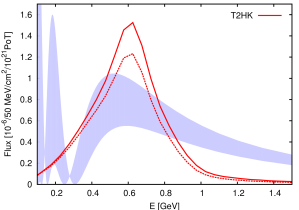
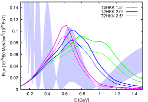
Figure 2: Left: T2HK’s flux plotted against neutrino energy for $\nu$-mode (solid) and $\overline{\nu}$-mode (dashed). Right: the T2HKK fluxes plotted against energy for $\nu$ and $\overline{\nu}$ modes. The shaded region shows the envelope of the probability found by varying the true value of $\delta$. Due to T2HKK’s longer baseline but comparable energy range to T2HK, the fluxes on the right sample a very different part of the probability.

The Tokai to Hyper-Kamiokande (T2HK) experiment [38] is the proposed next-generation long-baseline experiment using a neutrino beam produced at the synchrotron at J-PARC in Tokai directed $2.5\mathrm{°}$ off-axis to Hyper-Kamiokande (Hyper-K), a new water Čerenkov detector to be built near Kamioka, $295\text{\,}\mathrm{km}$ from the beam source. The narrow-band beam comprises mostly of $\nu_{\mu}$ (or $\overline{\nu}_{\mu}$), with the energy peaked near $600\text{\,}\mathrm{MeV}$ corresponding to the first oscillation maximum at $295\text{\,}\mathrm{km}$. Hyper-K is capable of detecting interactions of $\nu_{\mu}$, $\overline{\nu}_{\mu}$, $\nu_{e}$ and $\overline{\nu}_{e}$, allowing measurements of the oscillation probabilities $P(\nu_{\mu}\to\nu_{e})$, $P(\nu_{\mu}\to\nu_{\mu})$, $P(\overline{\nu}_{\mu}\to\overline{\nu}_{e})$, $P(\overline{\nu}_{\mu}\to\overline{\nu}_{\mu})$ with the primary goal of searching for CP violation and measuring $\delta_{CP}$.

The J-PARC neutrino beam will be upgraded from that used for the T2K experiment to provide a beam power of $1.3\text{\,}\mathrm{MW}$ [74, 75]. The beam is produced from $30\text{\,}\mathrm{GeV}$ protons colliding with a graphite target. Charged pions produced in these collisions are focused through magnetic horns into a decay volume, where the majority of the neutrinos in the beam are the $\nu_{\mu}$ ($\overline{\nu}_{\mu}$) produced from the $\pi^{+}$ ($\pi^{-}$) decay. The polarity of the $320\text{\,}\mathrm{kA}$ horn current can be reversed to focus pions of positive or negative charge in order to produce a beam of neutrinos or antineutrinos respectively. A small contamination (less than 1% of the neutrino flux) of $\nu_{e}$ or $\overline{\nu}_{e}$ in the beam and $\overline{\nu}_{\mu}$ ($\nu_{\mu}$) in the $\nu_{\mu}$ ($\overline{\nu}_{\mu}$) beam result from the decay of the $\mu^{+}$ ($\mu^{-}$) produced in the pion decay, however the majority of the $\mu^{\pm}$ are stopped after reaching the end of the decay volume before decaying.

The baseline design for the Hyper-Kamiokande detector consists of two water tanks each with a total (fiducial) mass of $258\text{\,}\mathrm{kt}$ ($187\text{\,}\mathrm{kt}$) [76]. Each tank is surrounded by approximately 40,000 inward facing $50\text{\,}\mathrm{cm}$ diameter photosensors corresponding to a 40% photocoverage, equivalent to that currently used at Super-Kamiokande. The tanks would be built and commissioned in a staged process with the second tank starting to take data six years after the first. The detectors use the water Čerenkov ring-imaging technique as used at Super-Kamiokande, capable of detecting the charged leptons produced in neutrino interactions on nuclei in water. At these energies, most neutrino–nucleus interactions are quasi-elastic, and the measurement of the outgoing charged lepton allows for an accurate reconstruction of the energy and flavour of the initial neutrino.

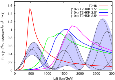
Figure 3: The T2HK and T2HKK fluxes shown as a function of $L/E$. The shaded region shows the envelope of the probability for $L=1100$ km and the black lines indicate the specific behaviour for $\delta\in\{0,\frac{\pi}{2},\pi,\frac{3\pi}{2}\}$. Note that the T2HK flux actually samples from the probability with a smaller matter effect corresponding to its shorter baseline $L=295$ km; however, on this scale the location of the first maximum does not deviate much from what is shown here.

We have developed an up-to-date GLoBES implementation of T2HK, incorporating the collaboration’s latest estimates for detector performance. Our simulation is based on the GLoBES implementation of T2HK [77] with comprehensive modifications to match the latest experimental design. The beam power and fiducial mass have been updated to $1.3\text{\,}\mathrm{MW}$ and $187\text{\,}\mathrm{kt}$ per tank. For our studies we have used the staged design with one tank operational for $6$ years followed by two operational tanks beyond that time. In cases where we show results against the run time of the experiment, we have used additional simulations with just a single tank operational throughout to highlight the discontinuous nature of this design. The neutrino flux and channel definitions have been updated to match those of Ref. [38], with separate channels for four interaction types (charged current quasielastic, charged current with one pion, other charged current and neutral current), for the $\nu_{\mu}\to\nu_{e}$ and $\overline{\nu}_{\mu}\to\overline{\nu}_{e}$ signals, and unoscillated $\nu_{e}$, $\overline{\nu}_{e}$, $\nu_{\mu}$ and $\overline{\nu}_{\mu}$ backgrounds. New tables of pre-smearing efficiencies and migration matrices have been created for each channel based on the full detector simulations used in Ref. [38]. New cross-sections for interactions on water for the four interaction types have been generated using the GENIE Monte-Carlo neutrino interaction event generator [78].

The simulation determines the event rates for signal and background components for each of $\nu_{\mu}/\overline{\nu}_{\mu}\to\nu_{e}/\overline{\nu}_{e}$ appearance and $\nu_{\mu}/\overline{\nu}_{\mu}\to\nu_{\mu}/\overline{\nu}_{\mu}$ disappearance measurements in neutrino mode and antineutrino mode. The rates are determined for 12 energy bins, given in Appendix A. For the appearance measurements, the energy range is restricted to $0\text{\,}\mathrm{GeV}1.25\text{\,}\mathrm{GeV}$, so only bins $18$ are included. All bins are included in the disappearance measurements. Separate uncorrelated systematic errors are assumed on the total signal and background rates for each of the four measurements, where the size of the errors assumed, summarised in Table 4, are the same as in the official Hyper-K studies after an adjustment to account for correlations between systematics not included in our simulations.

The design of T2HKK [39] and the location of the second detector module are still under development. As such, physics studies are being performed for a number of simulated fluxes with varying off-axis angles, generally ranging from on-axis to $2.5^{\circ}$ off-axis, which is aligned with the first detector in Kamioka. The novelty of this design is not only the longer baseline distance, which will enhance the role of matter effects, but also the fact that the energy profile of the flux remains similar to that at the detector at 295 km, meaning that the oscillation probability is sampled at very different values of $L/E$. This results in the second detector having access to increased spectral information, which can help to break degeneracies and enhance overall sensitivity [43]. This is clearly seen in Fig. 2, where the left panel shows how the flux aligns with the first maximum of the probability at Kamioka while the right panel shows that the fluxes align around the second maximum for the Korean detector. When plotted against $L/E$, as in Fig. 3, we see that the T2HK flux has only minor coverage of the second maximum in contrast to T2HKK. The fluxes used in our simulation were provided by the Hyper-Kamiokande proto-collaboration and were produced in the same way as the fluxes used in [38] but with a baseline of $1100$ km and off-axis angles of $1.5^{\circ}$, $2.0^{\circ}$ and $2.5^{\circ}$.

3.3 Experimental run times and $\nu$ : $\overline{\nu}$ ratios

The previous sections have discussed our models of the experimental details of DUNE and T2HK. However, in the present study, we will consider a number of different exposures for these experiments and their combination. This section is intended to clarify our terminology and explain our choices of run time, neutrino–antineutrino sharing, and staging adopted in the following analyses.

First, we comment that although the ratio of the run time between $\nu$ and $\bar{\nu}$ beam modes is also known to affect the sensitivities of long-baseline experiments, we stick to the ratios defined by each experiment’s official designs throughout our work. For DUNE and T2HK, the ratio of $\nu$ to $\bar{\nu}$ are 1:1 and 1:3, respectively. We have investigated the impact of changing these ratios, but they do not significantly impact the results, and for both experiments the optimal ratio was close to those assumed here. In the study for alternative designs, we stick with the same ratios as the standard configurations of DUNE and T2HK.

	Label	$\nu$ : $\overline{\nu}$ at DUNE	$\nu$ : $\overline{\nu}$ at T2HK
Fixed run time	DUNE	$5$ : $5$	0 : 0
	T2HK	0 : 0	$2.5$ : $7.5$
	DUNE + T2HK	$5$ : $5$	$2.5$ : $7.5$
Variable run time	DUNE	$T/2$ : $T/2$	0 : 0
	T2HK	0 : 0	$T/4$ : $3T/4$
	DUNE/2 + T2HK/2	$T/4$ : $T/4$	$T/8$ : $3T/8$

Table 1: The run times in years for each component of DUNE, T2HK, and their combination (DUNE + T2HK) for both the standard full data taking period (top 3 rows) and when considered with variable run times (bottom 3 rows). Plots with cumulative run time $T$ on the $x$-axis are for the “variable run time” configurations, whilst all other plots are for the “fixed run time” configurations. We specify the details for configurations without staged power or mass increases when relevant in the text. We note here that the fixed run-time configuration of DUNE (T2HK) corresponds to $600$ ($3400$) kiloton$\times$MW$\times$ years of exposure.

Most of our plots deal with three configurations labelled as DUNE, T2HK and DUNE + T2HK, and the sensitivities shown assume the full data taking periods for these experiments have ended. These are our standard configurations, and are defined in terms of run times and neutrino–antineutrino sharing in the rows labelled “fixed run time” in Table 1. We point out that as we are interested in comparing experimental performance, we take our standard configuration of DUNE to have 10 years runtime, equal to the baseline configuration of T2HK [38]. This does, however, differ from the 7 years considered in Ref. [21], and our sensitivities are correspondingly better.

However, we will also plot quantities against run time, and for these figures we define the sharing of run time between components in terms of a quantity we call the cumulative run time $T$; these are shown in the rows labelled “variable run time” in Table 1. The cumulative run time for the combination of DUNE and T2HK is defined to be the sum of the individual experiments’ run times, i.e. if the two experiments were run back to back, with no overlapping period of operation, then our definition of cumulative run time is identical to the calendar time taken for the full data set to be collected. Of course, if the experiments run in parallel, with identical start and end dates, our definition of cumulative run time would be double the calendar time required to collect the data. To remind readers of our definitions, we label this variable run time configuration as DUNE/2 + T2HK/2, as half of the cumulative run time goes to each experiment. Note also that, as per the official studies of each experiment, we assume $10^{7}$ seconds per year of active beam time for T2HK ($2.7\times 10^{21}$ POT/year at 1.3 MW with 30 GeV protons) and combined accelerator uptime and efficiency of 56% ($1.47\times 10^{21}$ POT/year at 1.07 MW with 80 GeV protons up to the 6th year, doubling the POT thereafter) for DUNE.

The possible staging options for the two modules of T2HK and the power of LBNF cause some added complication when plotting sensitivities against run time. In this study, we assume that our standard configurations of T2HK and DUNE follow the staging scenarios suggested by the collaborations: $6$ years of 1-tank ($187$ kt of total volume) running followed by $4$ with an additional tank for T2HK ($374$ kiloton of total volume), and $6$ years of $1.07$ MW ($1.47\times 10^{21}$ POT/year) followed by $4$ of $2.14$ MW ($2.54\times 10^{21}$ POT/year) for DUNE with 2-horn 80-GeV-proton design. In practice, we implement an effective mass for T2HK which depends on the run time $t$ assigned to T2HK defined by

$$M(t)=M_{0}\left[1+\Theta(t-6)\frac{t-6}{t}\right],$$

where $M_{0}$ is the mass of a single tank, defined above as $187$ kt, and $\Theta(x)$ is the Heaviside step function. We make an analogous definition for the power of DUNE, again increasing by a factor of two after 6 years. As our definition of cumulative run time $T$ would require 12 years to pass before 6 years of data had been collected by either of the experiments in the combination of DUNE/2 + T2HK/2, we see the discontinuity in sensitivity due to staging appear in two different places in our plots against run time: one for an experiment alone, and one for DUNE/2 + T2HK/2. This can be seen clearly in e.g. Fig. 5, where we mark the discontinuities with vertical dashed lines. So as to better understand the impact of these upgrades, we will also show the sensitivities against run time which would apply were they absent. However, we stress that the full programme of upgrades is an integral part of the collaborations’ proposals and should be taken as part of their baseline configurations.

Finally, in Section 5 we will deviate from these configurations (and the labels in Table 1) as we consider non-standard exposures for the purpose of better exploring the complementarity of DUNE and T2HK. This will be discussed in more detail in Section 5.

3.4 Statistical method

Our simulation uses GLoBES [67, 68] to compute the event rates and statistical significances for the experiments discussed in the previous section. We will now briefly recap the salient details of the statistical model underlying the analysis.

Given the true bin-by-bin event rates $n_{i}$ for a specific experimental configuration, we construct a $\chi^{2}$ function based on a log-likelihood ratio,

$$\chi^{2}(\vec{\theta},\xi_{s},\xi_{b})=2\sum_{i}\left(\eta_{i}(\vec{\theta},\xi_{s},\xi_{b})-n_{i}+n_{i}\ln\frac{n_{i}}{\eta_{i}(\vec{\theta},\xi_{s},\xi_{b})}\right)+p(\xi_{s},\sigma_{s})+p(\xi_{b},\sigma_{b}),$$ (3.1)

where $i$ runs over the number of bins, $\eta_{i}(\vec{\theta},\xi_{s},\xi_{b})$ is the hypothesis event rate for bin $i$ and $E_{i}$ is the central bin energy. The vector $\vec{\theta}$ has six components, corresponding to each of the three mixing angles, one phase and two mass-squared splittings of the hypothesis. The parameters $\xi_{s}$ and $\xi_{b}$ are introduced to account for the systematic uncertainty of normalization for the signal (subscript $s$) and background (subscript $b$) components of the event rate, and are allowed to vary in the fit as nuisance parameters. For a given hypothesised set of parameters $\vec{\theta}$, the event rate for bin $i$ is calculated as

$$\eta_{i}(\vec{\theta},\xi_{s},\xi_{b})=(1+\xi_{s})\times n_{i}+(1+\xi_{b})\times b_{i},$$

where $n_{i}$ and $b_{i}$ are the expected number of signal and background events in bin $i$, respectively. The nuisance parameters are constrained by terms $p(\xi,\sigma)=\xi^{2}/\sigma^{2}$, representing Gaussian priors on $\xi_{s}$ and $\xi_{b}$ with corresponding uncertainties $\sigma_{s}$ and $\sigma_{b}$. To test a given hypothesis against a data set, we profile out unwanted degrees of freedom. This amounts to minimising the $\chi^{2}$ function Eq. (3.1) over these parameters whilst holding the relevant parameters fixed. We will explain the statistical parameters of interest for each analysis in the following sections, however, as an example we will be interested in how well different hypothesised values of $\delta$ fit a given data set. In this case, we would compute

$$\chi^{2}(\delta)=\min_{\{\vec{\theta}\neq\delta,\xi_{s},\xi_{b}\}}\left(\chi^{2}(\vec{\theta},\xi_{s},\xi_{b})+P(\vec{\theta})\right),$$ (3.2)

where the notation $\vec{\theta}\neq\delta$ means all parameters other than $\delta$. The function $P(\theta)$ is a prior, introduced to mimic the role of data from existing experiments during fitting. In all fits that we perform, unless explicitly stated otherwise, we use true values from the recent global fit NuFit 2.2 (2016) [46]. $P(\theta)$ comprises a sum of the 1D $\chi^{2}$ data provided by NuFit for each parameter, except for $\delta$, and we switch between NO and IO priors depending on the mass ordering of our hypothesis. This includes the correlations which are currently seen in the global data, and our treatment goes beyond the common assumption of Gaussian priors, allowing for both the degenerate solution and its relative poorness of fit to be more accurately taken into account. The values of all parameters are permitted to vary, including the different octants for $\theta_{23}$, the value of $\delta_{CP}$ and the mass orderings, subject to the global constraints. Our choice of true values depends on the mass ordering, and are given explicitly in Table 2, unless stated otherwise. Note that the current best-fit values correlate the mass ordering and the octant, with NO preferring the lower octant and IO, the higher octant. This will affect our simulation, for example leading to poorer CPV sensitivity for IO, and in Section 4 we will show results for a band of $\theta_{23}$ spanning both solutions to mitigate this asymmetry.

We point out that our treatment of the external data, which attempts to accurately model the global constraints beyond the approximation of independent Gaussians, leads to some differences between our results and those of previous studies [21, 38, 44]. The differences can be traced to two key features: first, we take into account the significantly non-Gaussian behaviour of the global constraints at higher significances. This is particularly relevant for the prior on $\Delta m^{2}_{21}$ and we will comment on this in more detail in Section 4.1 and Appendix C. The second important feature of our priors is the strong correlation between mass ordering and the octant of $\theta_{23}$. The current global data disfavours the combination of IO and first octant (NO and second octant). This fact is reflected in our priors; although a visible local minimum is always present, it is never degenerate with the true minimum. In previous studies, various treatments of this degeneracy have been employed, some which do not allow the alternative minimum, and some which do not penalise it at all. Our method interpolates between these two extremes, and attempts to faithfully describe the current global picture. We will provide more detail on the specific differences between our results and existing calculations of the sensitivity of DUNE, T2HK and their variant designs on a case-by-case basis in the following sections.

Parameter	Normal ordering	Inverted ordering
$\theta_{12}$ [∘]	$33.72^{+0.79}_{-0.76}$	$33.72^{+0.79}_{-0.76}$
$\theta_{13}$ [∘]	$8.46^{+0.14}_{-0.15}$	$8.48^{+0.15}_{-0.15}$
$\theta_{23}$ [∘]	$41.5^{+1.3}_{-1.1}$	$49.9^{+1.1}_{-1.3}$
$\Delta m_{21}^{2}$ [$\times 10^{-5}$ eV2]	$7.49^{+0.19}_{-0.17}$	$7.49^{+0.19}_{-0.17}$
$\Delta m_{31}^{2}$ [$\times 10^{-3}$ eV2]	$+2.526^{+0.039}_{-0.037}$	$-2.518^{+0.038}_{-0.037}$

Table 2: The true values used in our fit, unless otherwise stated explicitly, with their uncertainties (the $1\sigma$ range of the priors we have used in our fit). These are based on NuFit 2.2 (2016) [46], and are similar to the parameters found in other recent global fits (see e.g. [79, 80]).

4 Sensitivity to mass ordering, CPV, non-maximal CPV, and octant

In this section, we will present the results of our simulation studying the sensitivity of the standard configurations of DUNE and T2HK. This means we use the 2-horn optimised flux for DUNE with a staged beam upgrade after 6 years, while for the T2HK detector we assume the installation of a second detector module after 6 years. More details of these configurations can be found in Section 3.1 and Section 3.2. However, for comparison, we also include two unstaged options: where the experiments continue without upgrading at the $6$ year mark. We stress that these are not the baseline configurations of the experiments, and that they are interesting for comparison purposes only. The run time and neutrino–antineutrino sharing for these configurations are discussed in more detail in Section 3.3. After considering these benchmark configurations and their complementarity, we will return to the potential of alternative designs in Section 6.

4.1 Mass ordering sensitivity

The mass ordering is one of the central goals of the next generation of LBL experiments; it is also one of the easiest to measure with this technology. We quantify the ability to determine the mass ordering by computing the following test statistic,

$$\Delta\chi^{2}_{\text{MO}}=\min_{\{\vec{\theta},\xi_{s},\xi_{b}\}}\left[\chi^{2}(\text{sgn}\Delta m^{2}_{31}=\text{true})-\chi^{2}(\text{sgn}\Delta m^{2}_{31}=\text{false})\right].$$ (4.1)

That is to say, the smallest value of the $\chi^{2}$ function for any parameter set with the wrong ordering. All parameters are allowed to vary during marginalisation whilst preserving the ordering. Although our composite hypothesis violates the assumptions of Wilks’ theorem [81, 82], and therefore invalidates the mapping between $\sqrt{\Delta\chi^{2}}$ and $\sigma$-valued significance for discrimination of the two hypotheses, we stick to convention in this section, reporting the expected sensitivities for the median experiment in terms of $\sqrt{\Delta\chi^{2}}$ and discussing it in terms of $\sigma$. For the reader who is interested in the precise formulation of the statistical interpretation of $\sqrt{\Delta\chi^{2}}$, see e.g. Ref. [83].

The sensitivity we find in Fig. 4 is very strong. DUNE, with its large matter effects, can expect a greater than $8.5\sigma$ measurement of the mass ordering after $10$ years for all values of $\delta$, with an average sensitivity of around $12\sigma$ and a maximal sensitivity of around $17\sigma$. T2HK alone has limited access to this measurement due to its shorter baseline, but can still expect a greater than $3\sigma$ measurement for around $25\%$ of the possible values of $\delta$ after $10$ years of data-taking. The combination of DUNE and T2HK running for 10 years each can reach sensitivities of at least $15\sigma$, with an average of around $18\sigma$. Care should be taken when interpreting such large significances; however, it is clear that DUNE, and the combination of DUNE and T2HK, can expect a very strong determination of the mass ordering. We also note the strong complementarity here: for the values of $\delta$ where DUNE performs the worst, the information from T2HK helps to raise the global sensitivity by about $7\sigma$. Despite this interesting interplay, the fact that this is such an easy measurement for experiments of this type, means that we will not dwell on the question of optimising such a measurement further.

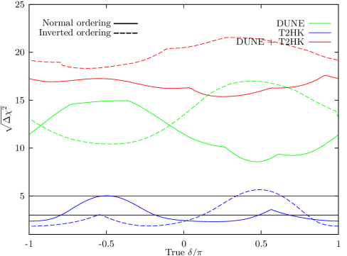
Figure 4: The sensitivity to the mass ordering for DUNE and T2HK in isolation and combined for true normal ordering (solid) and inverted ordering (dashed). This plot assumes the “fixed run time” configurations in Table 1 and the true oscillation parameters given in Table 2.

Our sensitivities in Fig. 4 deviate from previous published values for DUNE, and we generally report a worse ability for DUNE to exclude the ordering, with lower average sensitivity and visibly discontinuous behaviour in the values of $\Delta\chi^{2}$. This is due to the priors that we have imposed. Instead of a Gaussian approximation to the global data, we implement the global 1D $\chi^{2}$ functions, as provided by NuFit [46]. The true global data has strongly non-Gaussian behaviour at high significance, and there exist non-standard parameter sets which are not excluded at greater than $6\sigma$. These parameter sets sometimes become the best-fitting wrong-ordering solution, and must be excluded to rigorously establish the mass ordering. We discuss this in more detail in Appendix C. We point out, however, that our priors do not always significantly affect the point of minimum sensitivity, and DUNE still expects to see a greater than $5\sigma$ discovery for all true values of $\delta$. However, the values of parameters at the minimum do depend on our assumptions. For example, in Fig. 4 we have found for inverted ordering the lowest MO sensitivity over $\delta$ is affected by the degeneracy due to our prior, while for the normal ordering, the minimum is given by the conventional parameter set.

Another way to understand the complementarity of DUNE and T2HK is in terms of minimal run time necessary to ensure a $\sqrt{\Delta\chi^{2}}>5$ measurement regardless of the true value of $\delta$. We plot this quantity in Fig. 5, for normal ordering (left) and inverted ordering (right). The shaded bands take into account the variation in sensitivity due to the true value of $\theta_{23}$. DUNE alone takes between 2 and 6 years to reach this sensitivity, while the combination of DUNE and T2HK always takes less than 3 years (which if run in parallel is only 1.5 years). T2HK running alone cannot ensure a measurement of this significance over any plausible run time. We note the small discontinuity along the upper bound for normal (inverted) ordering after about 2 (5) years run time for DUNE. This marks the appearance of a degenerate solution due to the non-Gaussianity of our priors as discussed before (and in more detail in Appendix C). We also show explicitly the difference in minimal sensitivity for T2HK with (solid lines) and without (dashed lines) a second staged detector module at Kamioka, as well as for DUNE with (solid lines) and without (dashed lines) the upgraded accelerator complex. For T2HK, the increase in performance is negligible, but DUNE as well as the combination of DUNE and T2HK sees a notable performance increase.

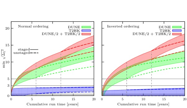
Figure 5: The least sensitivity for discovering mass ordering, $\text{min}(\sqrt{\Delta}\chi^{2})$, which can be reached by DUNE, T2HK and their combination as a function of cumulative run time. The width of the bands shows the sensitivity for $40^{\circ}\leq\theta_{23}\leq 50^{\circ}$. The left (right) panel assumes normal (inverted) ordering. These plots assume the “variable run time” configurations in Table 1 and the true oscillation parameters, apart from $\theta_{23}$, given in Table 2. The vertical lines mark the introduction of a staged second detector for T2HK and/or a increase in the beam power for DUNE. They lead to a notable discontinuity in sensitivity.

4.2 CP violation sensitivity

To fulfil the central aim of the LBL programme, the experiments must be able to rule out CP conservation over a large fraction of the true parameter space. This would imply a non-zero Jarlskog invariant and rigorously establish CP violation in the leptonic sector. Once again, we follow the conventional test statistic and define the quantity

$$\Delta\chi^{2}_{\text{CP}}=\min_{\delta\in\{0,\pi\}}\Delta\chi^{2}(\delta),$$ (4.2)

which amounts to studying the composite hypothesis of CP conservation ($\delta=0$ or $\delta=\pi$) [84]. Although at low-significance this test statistic is known to deviate from a $\chi^{2}$ distribution [85], we expect such effects to be small for the experiments under consideration in this study and the interpretation of $\sqrt{\Delta\chi^{2}}$ as $\sigma$-valued significances to be reasonable.

For the discovery of CP violation, the true value of the mass ordering and octant are relevant. We do not specify these values, and have studied the sensitivity for all combinations of values. We show in the left panel of Fig. 6 the significance for exclusion of CP conservation for the standard designs of the two facilities, in isolation and combination. We find that both experiments have a high sensitivity to this measurement, with at least a $3\sigma$ ($5\sigma$) discovery of CPV over $70$–$75\%$ ($46$–$47\%$) of the parameter space for DUNE and $73$–$80\%$ ($26$–$51\%$) for T2HK. For $0\leq\delta\leq\pi$, we see a notable difference in behaviour between DUNE and T2HK: the sensitivity for T2HK is limited, and much more dependent on the true value of $\theta_{23}$. This is due to the inability of T2HK to resolve the mass ordering degeneracy, which leads to a degenerate approximately CP conserving solution for these regions of parameter space. We point out that, as DUNE provides high MO sensitivity, the combination of data from DUNE and T2HK does not suffer from this problem, and sees significant improvements in sensitivity for these values of $\delta$. Aside from this limitation, the general shape of these curves can be understood by our discussion in Section 2.2. Discovery potential for CPV is closely related to the precision on $\delta$ at the CP conserving values, both rely on distinguishing between e.g. $\delta=0$ and other values. The best sensitivity to CP conserving values of $\delta$ is at the first maximum, where the majority of T2HK events are found and consequently it sees a better sensitivity. Our plots have assumed NO, but the qualitative picture remains the same for IO: in this case, the degeneracy occurs for the $-\pi\leq\delta\leq 0$, but otherwise the two regions of $\delta$ swap roles and the sensitivites are similar. We note, however, that the current best-fit values of $\theta_{23}$ would lead to additional suppression of CPV sensitivity for IO. The global data associates IO with a value of $\theta_{23}$ in the higher octant, which predicts poorer sensitivity to $\delta$.

As we mentioned in the last paragraph of Section 3.4, our prior correlates the allowed octant to the mass ordering, and this is responsible for differences between our results and previously published work. In Fig 6 of Ref. [44], there is almost no CPV sensitivity for $0<\delta<\pi$ for T2HK, which has not been found in our results, while their results for DUNE are similar to ours. This feature is explained as being due to the lack of MO sensitivity at T2HK, allowing for degeneracies to limit the sensitivity. In our simulation, however, T2HK alleviates this problem by its strong determination of the octant and the correlation of the global data. This lifts the degeneracy to higher significances, and allows a higher sensitivity to be obtained before the limiting effect becomes relevant.

We find that DUNE performs slightly better in our simulation than is reported in the left panel of Fig 3.13 in Ref. [21]. Around $\delta=\pi/2$ ($-\pi/2$), their result shows the sensitivity is about $5.8$ ($4.8$). However, our simulation finds a range of between $7.8$ to $9.0$ ($6$ to $8\sigma$) for $\delta=-\pi/2$ ($=\pi/2$). There are two sources for this discrepancy. Firstly, we are assuming a longer run time (10 years), for the purposes of comparison between T2HK and DUNE. Secondly, our priors are based on newer data, with updated central values and smaller $1\sigma$ intervals. The CPV sensitivity for DUNE does not peak around $\delta=-\pi/2$ in the left panel of Fig 3.13 in Ref. [21] like our results, due to the relatively poor determination of the octant. DUNE does not have as strong octant sensitivity as for the mass ordering, but our prior correlates the two, helping to reduce the impact of this alternative minimum for values of $\delta$ around $\delta=-\pi/2$. Finally, we find general agreement between our results and those of Fig. 119 in Ref. [38]. This is because the mass ordering is fixed during fitting in Ref. [38], which mitigates the impact of the mass ordering degeneracy. This leads to superficial agreement between our two sets of results when the degeneracy is not relevant, but discrepancies when it is. Our result shows the sensitivity which is possible assuming only the current global data, whereas assuming the MO is known would require new external data, perhaps from another long-baseline experiment (or from a joint analysis with atmospheric neutrino data).

In the right panel of Fig. 6, we show the fraction of values of $\delta$ for which a $5\sigma$ exclusion of CP conservation can be made as a function of run time. DUNE requires between $5$ and $7$ years of data-taking to reach at least a $5\sigma$ measurement for $25\%$ of the possible values of $\delta$, while T2HK alone shows a stronger dependence on $\theta_{23}$ but expects to be able to make at least a $5\sigma$ measurement for more than $25\%$ of the parameter space after $8$ years. The combination of DUNE and T2HK is shown as a function of cumulative run time, the sum of the individual run times for each experiment, and as such interpolates the two sensitivities. However, if run in parallel, the combination of the two experiments performs stronger than either in isolation, and expects a greater than $5\sigma$ measurement for more than $50\%$ of the parameter space after between $1.5$ and $2.5$ years of parallel data-taking.

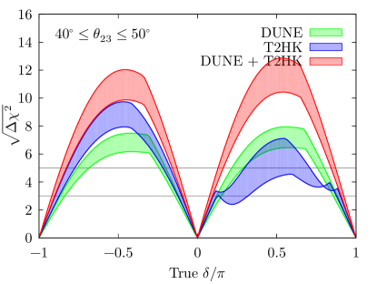
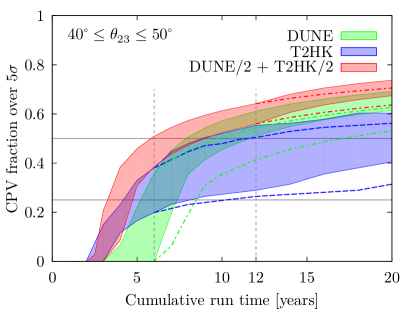
Figure 6: The sensitivity to CP violation for DUNE and T2HK in isolation and combined as a function of delta (left) and the fraction of $\delta$ parameter space for which greater than $5\sigma$ CPV discovery is expected (right). We consider a range of true $\theta_{23}$ spanning both octant solutions. The lower edge of the shaded regions corresponds to $\theta_{23}>45^{\circ}$ due to a decrease in sensitivity arising from the relative suppression of the CP sensitive terms in Eq. (2.1). The left (right) plot assumes the “fixed run time” (“variable run time”) configurations in Table 1 and the true oscillation parameters, apart from $\theta_{23}$, specified in Table 2.

4.3 Sensitivity to maximal CP violation

Although the search for any non-zero CPV is the principle goal of the next LBL experiments, understanding the value of $\delta$ is also highly relevant. Current global fits [46, 79, 80] point towards maximal values of $\delta$, $\delta=\pm\pi/2$. Of course, these should be treated with some scepticism: no single experiment can claim evidence for this at an appreciable level. However, determining if a maximal CP violating phase exists will remain a high priority for the next generation of long-baseline experiments. If established, it could be seen as an “unnatural” value advocated as evidence against anarchic PMNS matrices. Indeed, it is also one of the most common predictions in flavour models with generalised CP symmetries, and is often associated with close to maximal values of $\theta_{23}$ in models with residual flavor symmetries. For more discussion, see e.g.  Ref. [64, 65].

We have studied this question in Fig. 7 where we have defined the quantity

$$\Delta\chi^{2}_{\text{MCP}}=\min_{\delta\in\{-\frac{\pi}{2},\frac{\pi}{2}\}}\Delta\chi^{2}(\delta).$$ (4.3)

This is analogous to $\Delta\chi^{2}_{\text{CP}}$ defined earlier, and gives us a measure of the compatibility of the data with the hypothesis of maximal CP violation. On the left panel, we see the ability to exclude maximal CPV as a function of the true value of $\delta$. There is a similar sensitivity for both facilities. DUNE has the best performance for most cases, but T2HK still achieves the highest significance exclusions for $-3\pi/4<\delta<-\pi/2$ and $0<\delta<\pi/2$; although, its sensitivity is more affected by the value of $\theta_{23}$ and the mass ordering. In this way, the two experiments once again exhibit a complementarity, and the combination of DUNE and T2HK inherits the best sensitivity of its two component parts, expecting a $3\sigma$ exclusion of MCP for over $48$–$54\%$ of the parameter space.

On the right panel of Fig. 7, we show the fraction of true values of $\delta$ for which a $5\sigma$ exclusion of maximal CP violation can be achieved. By running in parallel for 10 years, DUNE and T2HK can expect a coverage at this significance of around $42$–$50\%$ of the parameter space. Once again we see T2HK’s sensitivity is more dependent on $\theta_{23}$ and generally lower than DUNE’s.

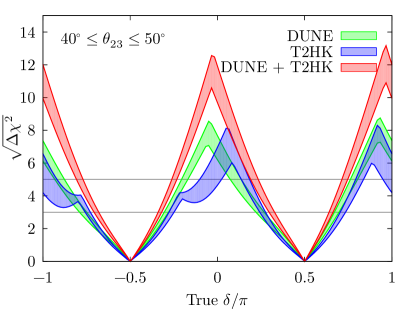
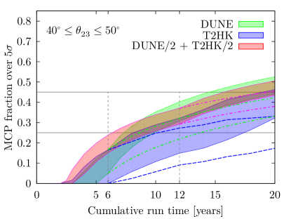
Figure 7: Left: the significance at which maximal CP can be excluded for DUNE and T2HK in isolation and combined as a function of true $\delta$. Right: the fraction of $\delta$-parameter space for which maximal CP can be excluded as a function of run time. The left (right) plot assumes the “fixed run time” (“variable run time”) configurations in Table 1 and the true oscillation parameters, apart from $\theta_{23}$, specified in Table 2.

4.4 Octant degeneracy and the precision on $\theta_{23}$

Although we know that $\theta_{23}$ is around $45^{\circ}$, the current global fit data allows for two distinct local minima, one below and one above $45^{\circ}$. This ambiguity is known as the octant degeneracy and arises as the disappearance channel of $\nu_{\mu}\rightarrow\nu_{\mu}$ is sensitive at leading-order only to $\sin^{2}2\theta_{23}$. However, the appearance channel breaks this degeneracy at leading-order, and future long-baseline experiments are expected to significantly improve our knowledge of $\theta_{23}$. In this section, we study how well DUNE and T2HK will be able to measure $\theta_{23}$ as well as settling two central questions: is $\theta_{23}$ maximal, and which is its correct octant? These questions are also of particular theoretical significance as many models with flavour symmetries exist which predict close to maximal values of $\theta_{23}$, and often the size of its deviation from this point is in correlation to other parameters like $\delta$ [64, 65]. Therefore, determining the octant (or maximality) of $\theta_{23}$ would be highly instructive in our search to understand leptonic flavour.

The ability to exclude the wrong octant for DUNE, T2HK and their combination is shown in Fig. 8. On the left, we show the sensitivity as a function of the true value of $\theta_{23}$. In these plots we assume a fixed value of $\delta=0$. The impact of varying $\delta$ for these measurements is small, as the degeneracy is broken at leading-order in the appearance channel, and the subdominant effects of $\delta$ are less relevant. The ability to exclude the wrong octant can reach up to 8$\sigma$ at the extremes of the current $3\sigma$ range of $\theta_{23}$, and we see that $3\sigma$ determinations of the upper (lower) octant can be expected for true values of $\sin^{2}\theta_{23}$ less than 0.47–0.48 (greater than 0.54–0.55). This corresponds to a $3\sigma$ determination of the octant for all values of $\theta_{23}$ in the ranges $\theta_{23}\lesssim 43.3^{\circ}$–$43.8^{\circ}$ or $\theta_{23}\gtrsim 47.3^{\circ}$–$48.4^{\circ}$. On the right, we fix the true value of $\theta_{23}$ and show how the sensitivity depends on cumulative run time. We see that the sensitivity quickly plateaus, and the staging options make little difference. Overall, the experiments expect to be able to establish the octant for this value of $\theta_{23}$ after only 2 to 4 years. Although this plot assumes $\theta_{23}=40^{\circ}$, changing the true value of $\theta_{23}$ leads to a predictable change in sensitivity, as indicated in the left panel, but does not qualitatively change the behaviour against run time. We see that overall, T2HK performs better than DUNE for the determination of the octant. However, the difference in performance is marginal, and their combination after 10 years of data for each experiment, outperforms T2HK running alone for 20 years, but performs slightly worse than DUNE with 20 year of total run time.

In this simulation, we have not imposed a prior on $\theta_{23}$. This process differs from Ref. [21], in which they give a gaussian prior for $\theta_{23}$. It also differs from the fitting method in Ref. [38], where they fit $\theta_{13}$, $\theta_{23}$ and the value of $\Delta m^{2}_{31}$ without implementing any priors, but fix $\theta_{12}$, $\Delta m^{2}_{21}$ and the mass ordering. In Ref. [44], the details of the fitting process are not specified. Despite these differences, we see qualitatively similar behaviour between the three sets of results. We find the regions of $\theta_{23}$ where the octant cannot be determined at $5\sigma$ to be $\theta_{23}\in[43^{\circ},49.7^{\circ}]$, $\theta_{23}\in[42^{\circ},48.9^{\circ}]$, and $\theta_{23}\in[43^{\circ},48.7^{\circ}]$ for DUNE, T2HK, and their combination, respectively. In Fig. 3.18 of Ref. [21], the equivalent region for DUNE is $\theta_{23}\in[41^{\circ},50^{\circ}]$, which is comparable to our work. In the middle panels of Fig. 5 in Ref. [44], the authors estimate the region as $42.5^{\circ}<\theta_{23}<48.5^{\circ}$ for T2HK and the combination of DUNE and T2HK, while for DUNE alone the range is slightly smaller than in our simulation at $42^{\circ}<\theta_{23}<49^{\circ}$. Compare to our results, in Fig. 125 of Ref. [38], we find the bigger range at $5\sigma$ level is $0.44<\sin^{2}\theta_{23}<0.58$.

In Fig. 9, we show the analogous plots for the exclusion of maximal $\theta_{23}$. We see that maximal $\theta_{23}$ can generally be excluded at greater significance than the octant. T2HK can reach $5\sigma$ sensitivity for $\sin^{2}\theta_{23}\lesssim 0.47$ as well as for $\sin^{2}\theta_{23}\gtrsim 0.55$, while DUNE can make an exclusion at the same statistical significance for $\sin^{2}\theta_{23}\lesssim 0.45$ and $\sin^{2}\theta_{23}\gtrsim 0.56$. Due to its poorer sensitivity, DUNE plays less of a role in the combination and DUNE + T2HK follows the sensitivity of T2HK. On the right, we show the sensitivity against cumulative run time. Again, the combination of DUNE + T2HK performs similarly to T2HK when the cumulative run time is divided by two, while DUNE performs slightly worse. We see that the staging of T2HK and DUNE plays a notable role, leading to significantly higher sensitivities.

We study the attainable precision on $\sin^{2}\theta_{23}$ in Fig. 10, where we plot $\Delta(\sin^{2}\theta_{23})$ against the true value of $\sin^{2}\theta_{23}$ for normal mass ordering. For all configurations, we see the same behaviour: the uncertainty climbs up from about $\sin^{2}\theta_{23}=0.48$ and falls down around $\sin^{2}\theta_{23}=0.54$, peaking at $\sin^{2}\theta_{23}\sim 0.51$. This is expected for a measurement dominated by the disappearance channel, where the probability is proportional to $\sin^{2}(2\theta_{23})$ and a leading-order analytic treatment would imply the relation

$$\Delta(\sin^{2}\theta_{23})\propto\left|\tan(2\theta_{23})\right|,$$

which naively predicts a total loss of sensitivity at maximal mixing, analogous to $\Delta\delta$ at $\delta=\pi/2$. This is mitigated by higher-order effects, as well as the information from the appearance channel, which becomes important around these values. The drop in sensitivity seen in Fig. 10 is quite sharp, and for values of $\sin^{2}\theta_{23}$ away from maximal mixing there is only modest variation in precision. For DUNE, $\Delta(\sin^{2}\theta_{23})$ is about $0.009$ at the boundaries, and peaks up to the value $\sim 0.038$. T2HK has better performance, with $\Delta(\sin^{2}\theta_{23})\sim 0.005$ for $\sin^{2}\theta_{23}=0.43$ and $0.585$. As with DUNE, the worst performance for T2HK is near the peak at $\sin^{2}\theta_{23}=0.5$ with $\Delta(\sin^{2}\theta_{23})\sim 0.032$. For significant deviations from $\theta_{23}=45^{\circ}$, the combination of DUNE and T2HK performs very similarly to T2HK, as T2HK’s high sensitivity drives that of the combination. However, the improvement of including DUNE data is viewable around the peak of $\Delta(\sin^{2}\theta_{23})$. In these plots, we set $\delta=0$, although qualitatively similar behaviour holds for other choices. There is, however, a correlation between the precision on $\theta_{23}$ and $\delta$. We present an estimate of the joint precision on $\theta_{23}$ and $\delta$ attainable at DUNE and T2HK in Fig. 11. In this plot, each ellipse shows the $1\sigma$ allowed region for a set of true values inside its boundary taken from the sets $\delta\in\{0^{\circ},\pm 90^{\circ},\pm 180^{\circ}\}$ and $\theta_{23}\in\{40^{\circ},45^{\circ},50^{\circ}\}$. T2HK generally performs slightly better for this measurement; although, at times DUNE achieves a marginally better sensitivity to $\delta$, and the combination of additional data from DUNE helps to reduce the T2HK contours. The best measurements will be obtained for large deviations from $\theta_{23}$-maximality and values of $\delta$ close to the CP conserving values, where DUNE (T2HK) can expect precisions on $\theta_{23}$ of $\Delta\theta_{23}=0.2^{\circ}$ ($\Delta\theta_{23}=0.13^{\circ}$). Conversely, the worst precision comes from the values of $\theta_{23}$ near maximal mixing where DUNE (T2HK) can expect larger uncertainties with $\Delta\theta_{23}=2^{\circ}$ ($\Delta\theta_{23}=0.95^{\circ}$). Comparing our result in Fig. 11 to Fig. 123 in [38], we find that our value for $\Delta\sin^{2}\theta_{23}$ is better than the official result for T2HK, which we suspect is due to the differences in our treatment of external data as mentioned previously.

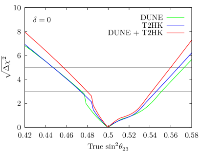
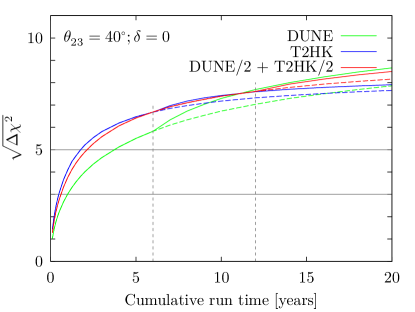
Figure 8: The sensitivity to exclude the wrong octant for DUNE, T2HK and their combination, as a function of $\sin^{2}\theta_{23}$ (left) and the cumulative run time (right). These plots assume $\delta=0$ and normal mass ordering. The left (right) plot assumes the “fixed run time” (“variable run time”) configurations in Table 1 and the true oscillation parameters, apart from $\theta_{23}$, specified in Table 2.

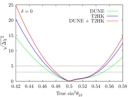
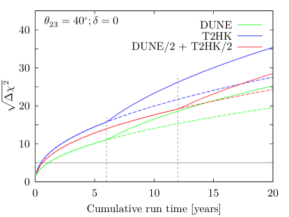
Figure 9: The ability to exclude $\theta_{23}=45^{\circ}$ for DUNE, T2HK and their combination, against the true value of $\sin^{2}\theta_{23}$ (left) and the cumulative run time (right). These plots assume $\delta=0$ and normal mass ordering. The left (right) plot assumes the “fixed run time” (“variable run time”) configurations in Table 1 and the true oscillation parameters, apart from $\theta_{23}$, specified in Table 2.

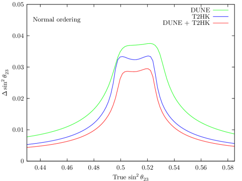
Figure 10: The expected 1$\sigma$ precision on $\sin^{2}\theta_{23}$ as a function of true value of $\sin^{2}\theta_{23}$ from $0.43$ to $0.585$ for DUNE, T2HK, and their combination, under the assumption of normal ordering. This plot assumes the “fixed run time” configurations in Table 1 and the true oscillation parameters, apart from $\theta_{23}$, specified in Table 2.

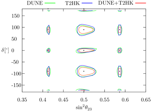
Figure 11: The attainable 1$\sigma$ precision on $\sin^{2}\theta_{23}$ and $\delta$ for DUNE, T2HK, and their combination. In each case, the contours enclose the assumed true values for $\theta_{23}$ and $\delta$, marked with a point. This plot assumes the “fixed run time” configurations in Table 1 and the true oscillation parameters, apart from $\theta_{23}$, specified in Table 2.

5 Complementarity for precision measurements of $\delta$

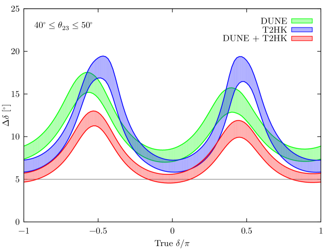
Figure 12: The $1\sigma$ precision on $\delta$ for DUNE and T2HK in isolation and combination. This plot assumes the “fixed run time” configurations in Table 1 and the true oscillation parameters, apart from $\theta_{23}$, specified in Table 2.

For the reasons outlined in Section 2.2, we expect an interesting interplay of sensitivities for a narrow-band and wide-band beam for the determination of $\delta$. In this section, we study the complementarity of DUNE and T2HK for precision measurements of $\delta$. In Fig. 12, we show the $1\sigma$ precision on $\delta$ which is attainable by the standard configurations of DUNE and T2HK and their combination. We consider a range of true values of $\theta_{23}$ as this significantly affects the ultimate precision. We see that for most of the parameter space T2HK can attain a better precision, with values of $\delta$ between $6$ and $7^{\circ}$ for the CP conserving values of $\delta$ compared to between $7.5$ and $9^{\circ}$ for DUNE. However, DUNE performs better than T2HK for maximally CP violating values of $\delta$ up to $5^{\circ}$. This leads to an effective complementarity between the two experiments, and their combined sensitivity reduces $\Delta\delta$ as compared to the two experiments in isolation by between $1$ and $6^{\circ}$ depending on the value of $\delta$.

We see therefore an improvement when combining the data from the two experiments. This was to be expected for a number of reasons. Firstly, there is a simple statistical benefit of combination — an increase in data reduces the statistical uncertainty and allows for a more precise measurement. On top of this, there is a synergistic benefit, where the two experiments mutually improve the reconstruction of the parameter of interest. To try to understand the synergy between DUNE and T2HK, we have run simulations where we mitigate the statistical advantage through different normalization procedures so as to expose the complementarity shown by the information available in each data set. As the experiments operate under such different assumptions, there is no universal way to do this. There are many factors which influence an experiment’s sensitivity: for example, the total flux produced by the accelerator; the effects of baseline distance on the flux; the detector’s size, technology and analysis efficiencies; not to mention the purely probabilistic effects of the oscillation itself, which occurs over different baseline distances and at different energies. In the next two sections, we consider different ways to normalise the experiments which reveal different aspects of their sensitivities.

5.1 Normalising by number of events

We can remove the statistical advantage of combining two experiments by fixing the number of events. We will consider two ways of doing this, both based on the total number of signal events $S$, composed of genuine appearance channel events in the detectors. We define $S$ to be the sum of these events across both neutrino and antineutrino mode appearance channels.

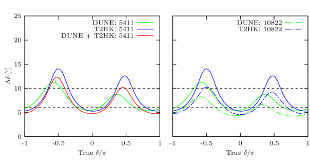
Figure 13: Left: the precision attainable by DUNE, T2HK and their combination with a fixed number (5411, the average number expected by DUNE + T2HK) of appearance channel events. On the left, DUNE + T2HK denotes the “fixed run time” configuration in Table 1, which expects around 5411 events. Right: the performance of DUNE and T2HK with double numbers of appearance events (in brackets) compared to those with 5411 events. In both plots, all unspecified parameters take the true values given in Table 2.

Our first normalization method fixes $S$. This is, of course, an unrealistic goal in practice. However, it answers an interesting hypothetical question: would a given number of events be more informative if they came from DUNE or T2HK? We have run the simulation of T2HK and DUNE while fixing the number of events in the appearance channel. This number varies with $\delta$, and so the effective run time has been modified for each value of $\delta$ to keep the observed events constant. In the left-hand panel of Fig. 13, we have fixed the number of appearance events to be 5411 for each configuration, which is the average number of events expected for the combination of DUNE and T2HK running for $20$ years cumulative run time. We see that events at DUNE are more valuable than events at T2HK around maximally CP violating values; however, around CP conserving values, the opposite is true and T2HK has more valuable events. We quantitatively assess this effect in the right-hand panel of Fig. 13. This plot compares the performance of DUNE and T2HK with a fixed 5411 events, with the same experiments assuming double the number of events. The figure shows that for DUNE to consistently outperform T2HK, it needs at least twice as many events. The same is true to T2HK: it can only lead to better performance for all values of $\delta$ once its has more than twice the exposure.

Our second normalization scheme is designed to include the effect of the probability from the comparison with fixed event rates. The number of appearance channel events, $S$, is to a good approximation proportional to the oscillation probability,

$$S\propto P(\nu_{\mu}\to\nu_{e};\langle E\rangle),$$

where $\langle E\rangle$ denotes the average energy of the flux, and we introduce a quantity $N$ denoting signal events with the effects due to the probability removed,

$$N(\langle E\rangle)=S/P(\nu_{\mu}\to\nu_{e};\langle E\rangle).$$ (5.1)

$N$ can be thought of as the constant of proportionality between the number of signal events and the probability, and it is affected by many factors, whose product is often referred to as the exposure of the experiment. These factors, such as run time, detector mass and power of the accelerator, describe technical aspects of the experimental design and the exposure is often taken as a proxy for run time in phenomenological studies of neutrino oscillation experiments. However, there are other factors affecting the coefficient $N$ such as the effects of cross-sections and detector efficiencies, which also vary from experiment to experiment. Our definition of $N$ accounts for all of the factors which affect the signal, apart from the fundamental effect of the oscillation probability. Equating $N$ assumes that all technical parameters are identical between the two experiments, and allows us to study the effect of the oscillation probability alone. We find that fixing $N$ leads to little change from fixing $S$. DUNE still outperforms T2HK for values of $\delta$ near maximal mixing, while T2HK performs best at CP conserving values. Even isolating the effect of probability in this way, we arrive at the same conclusion that events at DUNE are more informative about the value of $\delta$ than at T2HK around $\delta=\pm\pi/2$, while each event of T2HK has more impact than when $\delta$ is CP conserving.

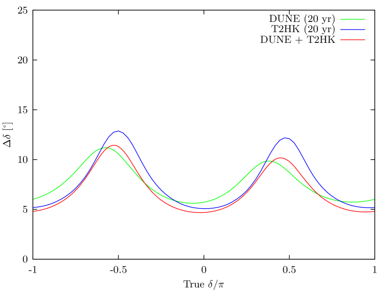
Figure 14: The 1$\sigma$ precision on $\delta$ as a function of the true value of $\delta$ for DUNE, T2HK and their combination with the same cumulative run time of 20 years. The configuration of DUNE (20 yr) is defined by the “variable run time” entry in Table 1, with $T$ given in brackets after the experiment’s name, whereas DUNE + T2HK is the corresponding “fixed run time” entry. Note that due to the staged upgrades of both designs, DUNE (20 yr) and T2HK (20 yr) correspond to 6 years without the planned upgrades followed by 14 years of upgraded running. This plot assumes normal mass ordering and all other unspecified true parameters are given in Table 2.

Comparing the expected precision on $\delta$ under our different normalization conditions gives us an idea of the role played by the probability. We see that generally, the conclusions are the same: when arranged to have equal normalizations, T2HK does worse than DUNE for maximal CP violation, but performs better at $\delta=0$ and $\pi$. This is true even if probability is included in the normalization, so we infer the difference in performance really does come from the spectrum. We conclude this section by noting that both normalization methods highlight the same aspect of the two experiments: for equal events the two experiments are very complementary, each providing the best measurement of $\delta$ for around half of the parameter space. However, in its standard configuration, DUNE expects fewer events than T2HK in the appearance channels. We will study this in more detail in the next section.

5.2 Normalising by run time

Of course, one of the most pragmatic ways to normalise the experiments is by run time. Would a decade of both experiments running in parallel be better than two consecutive decades of DUNE (or T2HK)? To make this comparison, we assume the same cumulative run time for the experiments running alone, and in combination. In Fig. 14 we show the results of our simulation. The combination of DUNE and T2HK generally outperforms either experiment running for twice as long. However, there are some small regions of parameter space around maximal CP violating values of $\delta$ where $20$ years of DUNE outperforms not only T2HK but also the combination of DUNE and T2HK. At these values of $\delta$, DUNE’s wide-band beam performs best by incorporating information from other energies. We also see this benefit in the combination of DUNE and T2HK, which notably outperforms $20$ years of T2HK at these values. This result tells us that the combination offers two advantages. First, running the experiments in parallel allows us to collect two decades of data in half the calendar time. This explains a significant part of the sensitivity improvement; however, there is also a complementarity arising from the different sensitivities of the two experiments. This is especially marked for this measurement around the maximally CP violating values of $\delta$.

The behaviour of $\Delta\delta$ for different experimental configurations as a function of run time is shown in Fig. 15. We have studied this for the maximum and the minimum values of $\Delta\delta$ (denoted $\Delta\delta_{\text{max}}$ and $\Delta\delta_{\text{min}}$), which describe the extremes of performance for the two experiments. We find that $\Delta\delta_{\text{max}}$ is better at DUNE than T2HK for all run times, whereas the situation is reversed for $\Delta\delta_{\text{min}}$. We note that for both experiments, the staged upgrades lead to a strong improvement in the sensitivity. If run in parallel, the combination of DUNE and T2HK expects $\Delta\delta_{\text{min}}<5^{\circ}$ and $\Delta\delta_{\text{max}}\lesssim 11^{\circ}$ after 10 years.

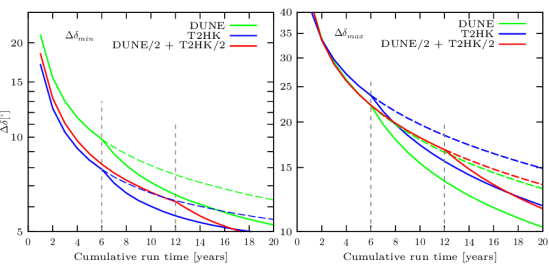
Figure 15: $\Delta\delta_{\text{min}}$ (left) and $\Delta\delta_{\text{max}}$ (right) at DUNE, T2HK and their combination as a function of run time. These plots assume the “variable run time” configurations in Table 1 and the true oscillation parameters appropriate for normal ordering as given in Table 2. We have checked that similar behaviour obtains for inverted ordering.

To end this section, we compare the performance of the two experiments and their combination through the minimal exposures required to obtain certain physics goals. In Table 3, we show the value of $N$, see Eq. (5.1), the number of signal events $S$ and the cumulative run time required to reach a precision on $\delta$ of $10^{\circ}$ for $\Delta\delta_{\text{max}}$ and $\Delta\delta_{\text{min}}$. It is clear from our study in this section that to achieve a precision of $10^{\circ}$ for $\Delta\delta_{\text{max}}$ will be a challenging measurement: above $20$ years of data is necessary, requiring $12.5$ years of both experiments running in parallel. For $\Delta\delta_{\text{min}}$ this is, however, a feasible goal. DUNE expects a similar measurement after a full $5.8$ year data-taking period, while T2HK can achieve this goal in $3.3$ years. The combination of DUNE and T2HK marginally improves on this, requiring only $1.9$ years of parallel running.

	$\Delta\delta_{min}$			$\Delta\delta_{max}$
	DUNE	T2HK	Both	DUNE	T2HK	Both
$\delta$	$354^{\circ}$	$0^{\circ}$	$0^{\circ}$	$255^{\circ}$	$270^{\circ}$	$264^{\circ}$
$N$	26837	15868	21900	167497	332532	218995
$S$	961	1034	739	6811	15653	8124
Cumulative run time [years]	5.8	3.3	3.8	21.1	27.1	25

Table 3: Exposures required for $\Delta\delta_{\text{max}}$ and $\Delta\delta_{\text{min}}$ to reach $10^{\circ}$. T2HK has the best precision on reasonable time scales due to its very high event rate especially at $\delta=\pi$. DUNE marginally out performs T2HK for maximally violating values of $\delta$. The year shown in this table, assumes the “variable run time” configurations of Table 1. The combination “Both” assumes a scaling of the standard configuration of DUNE/2 + T2HK/2.

5.3 Impact of systematic errors

In the previous section, we have looked at the precision on $\delta$ under a number of different assumptions. We have seen that T2HK has a larger number of events than DUNE, and for the majority of the parameter space this leads to a better expected precision on $\delta$. This means that the relationship between statistical and systematic uncertainty will be quite different at the different experiments and our assumptions about systematics, always a contentious issue, may be significant. In this section we try to understand these effects and explore the impact on the expected precision on $\delta$ under differing systematics assumptions for the combination of DUNE and T2HK.

We can get a feel for the relevance of statistical versus systematic uncertainty by seeing how the sensitivity scales with run time. In our model of the systematics, we only consider effective signal and background normalisation systematics for both DUNE and T2HK. In Fig. 16, we show the sensitivity to $\delta$ for different run times of the two experiments in isolation, with and without systematic uncertainties. We see that there is little impact from the systematic uncertainty at DUNE, and it continues to further its sensitivity as we increase its run time. This effect is quite different for T2HK where systematics clearly have a more important role; for CP conserving values, there is only modest improvement in sensitivity after extensions of the experiment run time by a factor of 4. This result neatly shows that DUNE is statistically limited while T2HK has more reliance on its systematic assumptions (except for maximally CP violating values of $\delta$). It is interesting to note that in both cases, even after large increases in exposure, neither DUNE nor T2HK taken as a single experiment can significantly improve on the sensitivity at CP conserving values found by the combination of DUNE and T2HK running for only 10 years each.

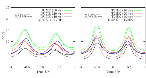
Figure 16: Left (right): the expected 1$\sigma$ precision on $\delta$ for DUNE (T2HK) with different run times with and without systematics (solid and dashed, respectively) compared to a reference design of our “fixed run time” configuration of DUNE + T2HK from Table 1. Note that in all cases, the experiments in isolation have a staged upgrade after 6 years, and so see increasingly long periods of upgraded running.

Due to the limiting effect of systematic uncertainties suspected at T2HK, we can expect that its performance is quite sensitive to our assumptions. To understand how the combination of DUNE and T2HK can help reduce this sensitivity, we have run simulations while varying the value of the normalization systematics in T2HK. We study the case of 2%, 4%, 6% and 8% normalization uncertainty at T2HK for the combination of DUNE and T2HK in comparison to T2HK running for 10 years with the same systematic assumptions. The results are shown in Fig. 17. We see that for $2\%$ systematic uncertainty, around $\delta=0$ and $\pi$, T2HK dominates the precision on $\delta$ and is limited strongly by the systematics, meaning that doubling the run time leads to scant improvement. As the systematic uncertainty on T2HK increases, we see more of an advantage of including DUNE. Although at $4\%$ systematics the lines are almost identical, for $6\%$ systematics the improvement in precision at $\delta=0$ is around $2^{\circ}$ (an improvement of around $10\%$). We conclude that T2HK is systematically limited around CP conserving values of $\delta$, and including DUNE data can help to mitigate the effect of larger uncertainties. At maximally CP violating value of $\delta$, we see little impact of our systematic assumptions.

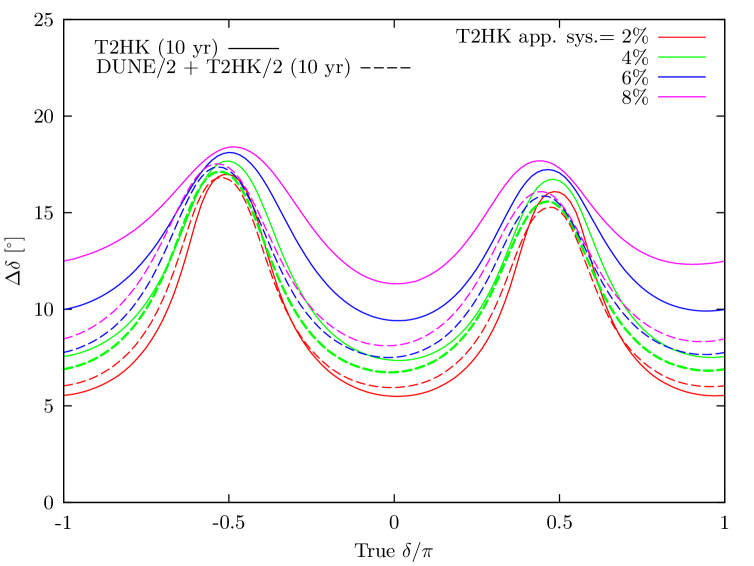
Figure 17: $\Delta\delta$ for T2HK and the combination of DUNE/2 + T2HK/2 each with 10 years cumulative run time for different normalization systematic uncertainties on the appearance channel in T2HK (2%, 4%, 6%, and 8%). We hold the normalization systematics at 2% for the appearance channels of DUNE. The configurations in this plot are labelled “variable run time” in Table 1 with the cumulative run time denoted in brackets after their names. This plot assumes normal ordering, but all other true parameters follow Table 2.

6 Impact of potential alternative designs

As part of their continual optimisation work, both the DUNE and T2HK collaborations have considered modifications of their reference designs, aiming to further the physics reach of their experiments. As mentioned in Section 3.1, DUNE has considered an optimised beam based on a 3-horn design, and a novel beam concept, nuPIL. For T2HK, the redesign efforts are focused on the location of the second tank. Originally foreseen as being installed at Kamioka 6 years after the experiment started to take data, the possibility of installing the detector in southern Korea has been mooted [40, 41, 42, 43]. In this section, we discuss the impact of these redesigns on the physics reach of the experiments, both alone and in combination, via the results of our phenomenological discussion and simulations. We focus on the mass ordering, CPV discovery, MCP and precision measurements of $\delta$. We point out that we do not discuss measurements of $\theta_{23}$ further, as we have found that there is little difference between the alternative designs under consideration.

6.1 Experimental run times and $\nu$ : $\overline{\nu}$ ratios

In all plots that follow, we assume that DUNE and its variants will run with equal time allocated to neutrino and antineutrino mode, while T2HK and T2HKK will always follow the 1:3 ratio of their standard configuration. We also assume that there is no staged implementation of any of the variants of T2HKK, and that both detector modules start collecting data at the same time. For DUNE and the lines labelled T2HK, we assume our standard configurations which implement a staged upgrade at 6 years. Note that this means that when comparing T2HKK with DUNE or the single-tank T2HK, T2HKK benefits from an increase in exposure.

The run time configurations for these alternative designs follow those of the “variable run time” options in Table 1, albeit with variant fluxes for each experiment. All variants of DUNE, T2HK and T2HKK when run on their own are assumed to have a cumulative run time of 10 years. When a variant of DUNE is run in combination with a variant of T2HK, we assume that the cumulative run time is divided equally between the two experiments in the same way as DUNE/2 + T2HK/2 in Table 1. This means that when not plotted against $T$, the combination of DUNE and T2HK will have $T=20$, corresponding to 10 years running time for each of the two experiments.

6.2 Mass ordering

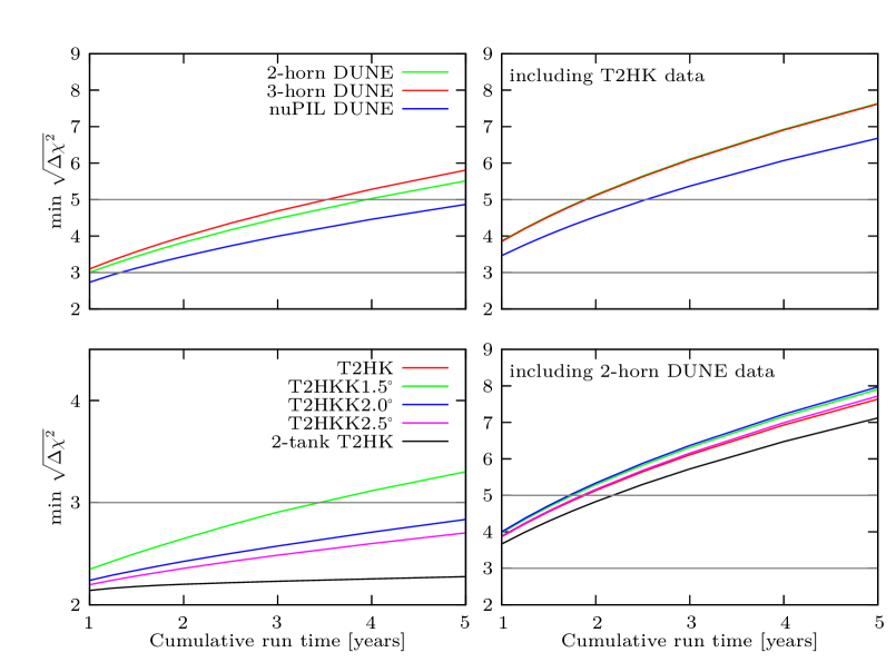
Figure 18: Top (bottom) row: The minimum statistical significance of mass ordering discrimination for DUNE (T2HK) with various beam designs. On both rows, the left-hand panels show the performance of the alternative designs in isolation, while the right-hand panels show the impact of an alternative design on the combination of DUNE and T2HK by incorporating the standard T2HK and DUNE designs on the top and bottom rows, respectively. The configurations assumed here are described in Section 6.1 and the true oscillation parameters are given in Table 2. Full details of the assumed exposures can be found at the start of Section 6.1, and that in the top-right panel, the blue and green lines overlap.

As shown for the standard configurations in Section 4.1, identifying the mass ordering is almost guaranteed for experiments on this scale. However, we see a large difference in performance between DUNE and T2HK due to the difference in baseline distance. The alternative beams of the DUNE collaboration do little to change this picture. The results of our simulation are shown in Fig. 18, in which we show the minimum sensitivity to the mass ordering as a function of cumulative run time. The left column of panels shows the performance of the alternative designs for DUNE (top) and T2HK (bottom). We see that for DUNE, the 3-horn and 2-horn designs do better at the minimum sensitivity by about $1\sigma$ compared to the nuPIL design. We see that the 3-horn design can reach greater than $5\sigma$ significance after around $3.3$ years run time, while the 2-horn design achieves the same significance after around 4 years, and nuPIL requires above $5$ years. For T2HK and its alternative designs the picture is quite different. The T2HK design cannot achieve sensitivity above $2\sigma$ for these run times. However, placing a second tank in Korea will allow T2HKK to see larger matter effects over the $1000$–$1200$ km baseline: the sure-fire way to sensitivity to the mass ordering. Moreover, the possibility of placing the second detector at a different off-axis angle, could produce a wider beam, or a narrow beam whose peak is shifted away from the first maximum. This interplay of factors could qualitatively alter our picture of mass ordering sensitivity at HK(K). We see a greater variation in performance as the fluxes are varied, but as we saw before, lower overall sensitivities. Due to the larger matter effects associated with the Korean detector, we might expect increased sensitivity to the mass ordering over the standard T2HK design; however, we do not see an enhancement of this kind. We understand this effect as due in part to the limited data collected by T2HKK at the longer baseline. Fewer events associated with neutrinos travelling the longer baseline are detected as the beam suffers significant suppression due to dispersion over the longer distance as can be seen in Table 5. With WC technology, we know that the advantage comes from scale, and such a limitation on event numbers means that longer baselines will not be competitive unless operated for a longer period of time. Moreover, the matter effect is relatively suppressed compared to the effect at DUNE due to the lower energies of the J-PARC beam. And it has been shown in Ref. [43] that it is not sufficient to allow for a separation of the two degenerate solutions in all cases at fixed energies. However, the most important contribution of a Korean second detector is the very different spectral information it provides from a detector at Kamioka. This helps to provide sensitivity to the ordering, and we see that the T2HKK$1.5^{\circ}$ option expects to push the sensitivity above $3\sigma$ after around $3$ years. Although we do not show the full MO sensitivity against $\delta$ in Fig. 18, we can draw a limited comparison between our work and Fig. 18 in Ref. [39]. Our results find slightly lower sensitivities: for T2HKK$1.5^{\circ}$, the difference is about $1\sigma$, while for off-axis angles of $2.5^{\circ}$ and $2.0^{\circ}$ the difference is smaller than $1\sigma$.

The sensitivity is seen to increase as the Korean detector is moved to smaller off-axis angles. This can be explained by the different flux profiles of the T2HKK options. As the detector is moved towards the beam axis, the events sample the oscillation probability increasingly close to the first maximum. This is where the mass ordering is most visible in the presence of matter effects and we see an accordingly stronger discovery potential.

On the right column of Fig. 18, we show how the alternative designs impact the combination of the two experiments. Including T2HK data reduces the difference in performance between the three DUNE beam designs, which all expect a minimum sensitivity of $5\sigma$ after about $2$ years. For T2HK, the inclusion of DUNE data, pushes the overall sensitivity above $5\sigma$ for the first time, with an extra Korean detector, DUNE + T2HKK expects a greater than $5\sigma$ measurement for all values of $\delta$ with around $2$ years run time.

6.3 CPV and MCP sensitivity

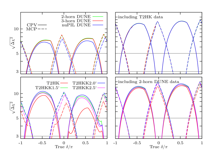
Figure 19: The sensitivity to CPV (solid) and MCP (dashed) as a function of $\delta$ for various designs of DUNE (top row) and T2HK (bottom row). The exposures assumed here are described in Section 6.1 and the true oscillation parameters are given in Table 2.

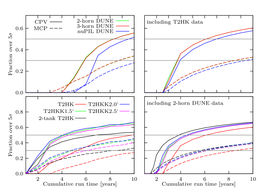
Figure 20: The fraction of true $\delta$ values for which we expect a CPV sensitivity (solid) and MCP sensitivity (dashed) over 5 $\sigma$, against cumulative run time. The exposures assumed here are described in Section 6.1 and the true oscillation parameters are given in Table 2.

The sensitivity to CPV is understood to depend upon the energy of the events observed, meaning that modifying the flux spectrum, for example with a narrower beam from nuPIL or a beam located at the second maximum for T2HKK, could lead to significant changes in the physics reach of the design. In the top-left panel of Fig. 19 we compare the performance of the standard and alternative DUNE designs. CPV and MCP sensitivities are shown for the three beam options as a function of $\delta$ in solid and dashed lines, respectively. We find that the 2-horn and 3-horn designs perform similarly for CPV and MCP measurements, and nuPIL performs slightly worse, by about $1\sigma$. The top-right panel shows how these sensitivities are changed as information from the standard configuration of T2HK is included. We see that due to T2HK’s strong sensitivity to the parameter $\delta$, the impact of alternative designs for DUNE is greatly reduced. Maximal sensitivities to CPV of above $11\sigma$ are found for the maximal values of $\delta\in\{\frac{\pi}{2},\frac{3\pi}{2}\}$.

For T2HKK we compare three off-axis angles for the Korean detector to the standard configuration in the bottom row of Fig. 19. On the left panel, we show the performance of these alternative designs in isolation. We see that the experiments perform comparably, but the best performance comes from the T2HKK2.0^∘ flux. As can be seen in Fig. 3, this flux is the best aligned with the second maximum, suggesting that it is the access to events which sample this part of the oscillation spectrum which lead to the increase in sensitivity. The increase in sensitivity for $-\pi\leq\delta\leq 0$ is modest between T2HK and T2HKK. We understand this again due to the suppression in event rates for a Korean detector: although possessing valuable information, they are seen in relatively small numbers, and their impact is limited. However, there is a notable difference for $0\leq\delta\leq\pi$, as the Korean detector helps to lift the degeneracy which limits the performance of T2HK. In the bottom-right panel of Fig. 19, we see the sensitivity to CPV and MCP for combinations of DUNE and T2HKK. In these simulations, the degeneracy is lifted by the inclusion of DUNE data, and there is little difference between the alternative designs for T2HKK aside from an overall improvement in the sensitivities by between $1$ and $2\sigma$.

In Fig. 20, we have computed the fraction of values of $\delta$ for which CP conservation or maximal CP violation can be excluded at greater than $5\sigma$ confidence. The top-left panel shows the performance of the alternative DUNE beam designs in isolation. The 3-horn and 2-horn designs have almost identical sensitivities for all run times, with a CPV fraction greater than that of nuPIL by between $10$–$30\%$ and an MCP fraction higher by around $10\%$. If we consider $30\%$ to be a benchmark CPV fraction, the 3-horn and 2-horn designs expect to reach this sensitivity after around $5$ years, while nuPIL takes around $7$ years. Excluding MCP is a harder measurement for all beam designs, and exposures of greater than $10$ years would be required to achieve a $30\%$ coverage of $\delta$ parameter space at $5\sigma$. The top-right panel shows how the alternative DUNE designs are affected by the inclusion of T2HK data. Thanks to the good CPV and MCP sensitivity of T2HK, we see the improvement for the combination, especially for nuPIL by up to $10\%$. We also find a relative suppression of the difference between variants — ultimately, DUNE offers less to this configuration and its precise design is less important. These combinations expect to reach a CPV fraction of $30\%$ ($50\%$) after about $4$ ($6$) years. For the exclusion of MCP, a $30\%$ fraction will be approximately reached after 9 years run time.

The bottom row of Fig. 20, shows analogous plots for T2HK and T2HKK. On the left, these alternative designs are considered in isolation, and we have also included a 2-tank T2HK line for comparison which assumes two tanks collecting data at Kamioka from the start of the experiment. There is very little difference between the T2HKK designs, although they all show an increase in CPV and MCP fraction over the T2HK design. T2HKK expects a CPV fraction of over $50\%$ after less than $4$ years, while T2HK requires around $10$ years for the same sensitivity (and 2-tank T2HK around $7$ years). MCP fractions of greater than $30\%$ are possible after $5$ and $11$ years for T2HKK and T2HK, respectively. Compared with the results shown in the upper panels in Fig. 20 in Ref. [39], we find the same ranking of designs. However, we also find sensitivities around $2\sigma$ higher near $\delta=\pm\pi/2$. We suspect this quantitative difference is due to our priors, as in Ref. [39], it is pointed out that priors for $\delta_{CP}$, $\theta_{23}$ and $\Delta m^{2}_{31}$ are not implemented. However, we use priors on all variables apart from $\delta$, and our simulation has slightly less leeway to accommodate degenerate solutions, and a correspondingly improved ability to exclude CP conserving parameter sets. It is interesting to point out that, for both DUNE and T2HK, differences in design have a greater impact on the highest sensitivity to CPV and MCP, as seen in Fig. 19, than on the long-term average performance encapsulated in the CPV/MCP fraction at $5\sigma$. This can be seen in Fig. 19 as the width of the sensitivity curves remaining unchanged, while the peak is raised or lowered. The sensitivity of the peak corresponds to different rising behaviour in Fig. 20, but the curves can be seen to quickly plateau for T2HK. For DUNE, this effect is less marked, and suggests increasing run time would still lead to increases in sensitivity.

On the right panel, we show the performance for the combination of DUNE data with the T2HK variants. As in the bottom-left panel, we see that the T2HKK designs perform similarly, with T2HKK2.0 performing marginally better. The inclusion of DUNE data here makes little change to the sensitivities. In fact, as we define cumulative run time as the sum of the individual DUNE and T2HKK run times, we see an apparent decrease in performance. Scaled appropriately for parallel data collection, we find that DUNE + T2HKK expect a $5\sigma$ CPV fraction of greater than $50\%$ after around $2$ years compared to $4$ years for T2HKK alone. We note that there is a notable change in the performance of the T2HK design with two tanks at Kamioka operated for the duration of the experiment. Without DUNE data, this configuration performs more poorly than the T2HKK designs; however, with the inclusion of DUNE data, it becomes the best option. This can be understood as DUNE resolving the degeneracy and T2HK maximising its CPV measurement by a large increase of data at shorter baselines.

To conclude this section, we note that almost all of the experiments, when running in isolation, can expect the exclusion of one of CP conservation or maximal CP violation for all values of $\delta$ at $4\sigma$ and $5\sigma$ for DUNE and T2HK variants, respectively. This can be seen clearly in Fig. 19, where the intersections between CPV and MCP lines are above the $3$ or $5\sigma$ horizontal lines. This is true for all alternative designs, while the combination of DUNE and T2HK ensures that one of these facts would be established with a significance greater than $6\sigma$. The exception is for T2HK alone which, due to the degeneracy, falls short in some some regions of parameter space.

6.4 Precision on $\delta$

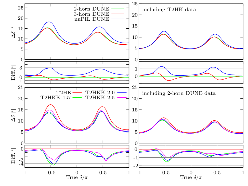
Figure 21: The 1$\sigma$ precision on $\delta$ for variants of DUNE (top row) and T2HK (bottom row). In the left column, these designs are considered in isolation while on the right, we combine variant designs of one experiment with the standard configuration of the other. Our configurations are described in Section 6.1. These plots assume normal mass ordering and the remaining true parameters are specified in Table 2.

We show the difference in $\Delta\delta$ for the alternative designs in the left column of Fig. 21. We find that for DUNE, the 3-horn design works similarly to 2-horn design; although, the 3-horn design performs slightly better in the 2nd and 4th quadrant and for maximal CP violation, while the 2-horn design expects smaller $\Delta\delta$ in all other cases. These designs expect a precision on $\delta$ somewhere between $8$ and $18^{\circ}$ after their full data taking period. The performance of the nuPIL design depends significantly on the true value of $\delta$. For values near maximal CP violation $\delta=\pm\frac{\pi}{2}$, nuPIL performs worse than the standard design. This can be understood due to the narrowing of the beam, which when focused on first maximum, has insufficient events from other energies to mitigate the poor sensitivity around maximal CP violating phases. On the top-right panel of Fig. 21, we show the impact that the DUNE redesigns have on the combination of DUNE and the standard configuration of T2HK. As shown in Section 5, data from T2HK improves the resolution on $\delta$ for DUNE, and we see a correspondingly small impact of alternative beam designs for DUNE. Notably, we do however see the worsening of performance around maximal CP violating values of $\delta$ for the combination of nuPIL and T2HK.

The expected sensitivity of $\Delta\delta$ for the alternative designs for T2HKK are shown on the bottom-left panel of Fig. 21. Here we see that all designs with a far detector allow for a significant improvement in the precision on $\delta$, generally seeing the best performance coming from the $1.5^{\circ}$ or $2.0^{\circ}$ off-axis angle fluxes. We see a slight loss of performance for larger off-axis angles, which may be associated with the peak of the flux falling beyond the second maximum into a region of hard to identify, fast oscillations. Our result for $\Delta\delta$ is very close to that shown in the upper panels of Fig. 23 in Ref. [39], and we agree on the ranking among alternative designs. This is notable, given the differences induced by our priors in other variables of interest, but is explained by the fact that our priors differ in their global structure more than in their local structure. It is this local structure which dictates $\Delta\delta$, as at low significance the Gaussian approximation works well and multiple minima are irrelevant. On the right panel of Fig. 21, the combination is shown with different T2HKK fluxes and the standard DUNE configuration. Once again, we see that T2HKK dominates the combination, and therefore the shapes of these curves closely follow those on the left panel.

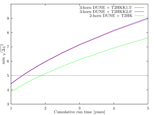
Figure 22: The minimum mass ordering sensitivity for the combination of DUNE with the 3 horn flux and T2HKK$1.5^{\circ}$ (red) and T2HKK$2.0^{\circ}$ (blue) compared with the standard configurations of DUNE with 2-horn flux and T2HK with a single tank at Kamioka (green). The configurations assumed here are described in Section 6.1 and the true oscillation parameters are given in Table 2.

6.5 Optimal configuration

In the preceding sections, we have studied how the alternative designs of T2HKK and DUNE could impact the physics reach for key measurements, considering both the experiments in isolation and in certain combinations. We have seen that for DUNE, the 2-horn and 3-horn designs perform similarly, with the greatest difference occurring for the measurements of the mass ordering and $\Delta\delta$. Both designs still expect very high significance measurements of the mass ordering. However, as we see in Fig. 12, the 3-horn design can achieve marginally better values of $\Delta\delta$ when $\delta$ in the 2nd and 4th quadrants, which is where T2HK performs worse than DUNE. We therefore take the 3-horn design to be the optimal choice for DUNE, with the 2-horn a close second. T2HKK in contrast performs best with a flux positioned between $1.5$ and $2.0^{\circ}$ degrees off axis. Here it maximizes its sensitivity to CP violation, its ability to exclude maximal CP violation and to make precision measurements of $\delta$ around CP conserving values. Whereas so far we have only considered alternative designs for one experiment in combination with the standard design of the other, in this section we report the physics reach of the optimal combination of DUNE 3-horn and T2HKK1.5 (and T2HKK2.0).

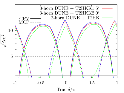
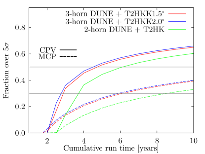
Figure 23: Left: the CPV and MCP sensitivity for the combination of DUNE with the 3-horn flux and T2HKK$1.5^{\circ}$($2.0^{\circ})$. For reference, we also show the combination of the two standard designs: DUNE with 2 horn beam and T2HK (green). Right: the fraction of $\delta$ parameter space for CPV (MCP) sensitivity over $5\sigma$ for the same configurations as on the left panel. The configurations assumed here are described in Section 6.1 and the true oscillation parameters are given in Table 2.

In Fig. 22, we show the minimum sensitivity expected for the mass ordering for this optimal configuration of DUNE + T2HKK. A $4\sigma$ measurement is expected after less than a year, which increases to $5\sigma$ after 1.5 years. In Fig. 23, we show the significance at which we can expect to exclude CP conservation (solid) and maximal CP violation (dashed). These are expected to reach a maximal significance of $11\sigma$ and $12\sigma$, respectively. The advantage of the combination is clearer when the performance is viewed in terms of the minimal run time required for the exclusions to be made at $5\sigma$. The combination of DUNE + T2HKK expects to have greater than $5\sigma$ exclusion of CP conservation for more than $25\%$ ($50\%$) of the parameter space after $2.5$ ($5$) years of cumulative run time. For the exclusion of maximal CP violation, longer run times are required: about $6$ years ensures the exclusion for more than $25\%$ of values of $\delta$. For the precision on $\delta$, shown in Fig. 24, we see that the optimal combination of DUNE + T2HKK could expect a measurement around a CP conserving value with an uncertainty of only $4.5^{\circ}$. This worsens for maximally CP violating values of $\delta$ to around $10^{\circ}$.

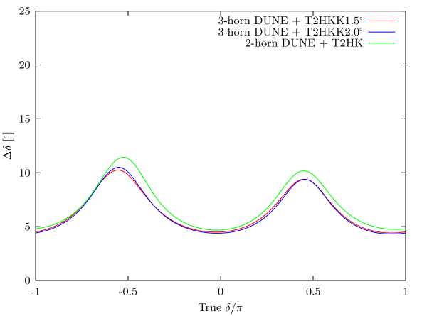
Figure 24: The $1\sigma$ error on $\delta$ for the combination of DUNE with the 3-horn flux and T2HKK$1.5^{\circ}$($2.0^{\circ}$) shown in red (blue). For reference, we also show the combination of the two standard designs: DUNE with 2-horn beam and T2HK with one tank (green). The configurations assumed here are described in Section 6.1 and the true oscillation parameters are given in Table 2.

7 Conclusions

DUNE and T2HK will lead the way in key measurements of the neutrino oscillation parameters. These long-baseline experiments will make high statistics determinations of the mass ordering, the first precision measurements of $\delta$, and have an excellent chance to establish the presence of fundamental CP violation in the leptonic sector. In this article, we have studied the expected performance of these two experiments, including possible alternative designs which have been recently suggested. We see that, thanks to their different designs, both the energy profiles of the beam and the different baseline distances chosen, DUNE and T2HK have different sensitivities to the mass ordering and the value of $\delta$, leading to a natural complementarity.

DUNE, with its long baseline and significant matter effects, excels at measuring the mass ordering. It can expect a greater than $5\sigma$ determination after between $2$ and $6$ years depending on the true value of $\theta_{23}$. T2HK is limited in its sensitivity for this measurement, but the combination of data collected at T2HK with the DUNE data reduces the impact of the worst-case scenario, significantly reducing the required run times. DUNE + T2HK can expect the same measurement in less than $3$ years regardless of $\theta_{23}$. The roles are reversed for measurements of the CP phase $\delta$. Although T2HK has high sensitivity for this measurement, it suffers from a degeneracy linked to the mass ordering which may limit its performance for some values of $\delta$. In isolation, T2HK expects to be able to exclude CP conservation at greater than $5\sigma$ for more than $50\%$ of the parameter space after around $5$ years in the best case scenario. DUNE alone would require at least $11$ years of data for the same measurement, but the combination of the two experiments, assumed to collect data in parallel, would take at most $5$ years. This is a particularly clear example of synergy between the two designs, as the degeneracy limiting T2HK’s sensitivity can be lifted by the inclusion of DUNE data. A similar but less pronounced synergy is present for the measurement of maximal CP violation, where the MO degeneracy again affects T2HK’s sensitivity. However, the combination of DUNE + T2HK mitigates this limitation and can exclude MCP for between $42$–$50\%$ of the parameter space after 10 years parallel data taking. For the measurement of the octant sensitivity, we find that to exclude the upper octant solution at 5$\sigma$ with a true value of $\theta_{23}=40^{\circ}$, T2HK needs about 2 years, while DUNE requires a slightly longer run time. This pattern is repeated for the exclusion of maximal mixing, where for the true value $\theta_{23}=40^{\circ}$, $5\sigma$ exclusion at DUNE takes around 2 years, while T2HK can make this exclusion in only 1 year. For these measurements, the performance of the combination of DUNE and T2HK generally follows the sensitivity of T2HK, although some small benefit is found from the inclusion of extra data. We have also studied the precision on $\sin^{2}\theta_{23}$, where there is a strong dependence on the true value of $\theta_{23}$, with the worst precision close to maximal mixing, as expected for a measurement driven by the disappearance channel. At the peak, $\Delta(\sin^{2}\theta_{23})$ for DUNE is about $0.041$ while T2HK can improve this, peaking around $0.032$. Extending our study to the 1$\sigma$ joint precision on $\delta$ and $\sin^{2}\theta_{23}$, we see the measurement to these two parameters are largely independent, due to the disappearance channel driving the fits to $\theta_{23}$ and the appearance channel dictates $\delta$. The precision gets worse at $\theta_{23}=45^{\circ}$, as seen before, and improves as we move from this maximal value. For $\theta_{23}=40^{\circ}$ or $50^{\circ}$, the precision on $\theta_{23}$ is around $0.2^{\circ}$ ($0.13^{\circ}$) for DUNE (T2HK). However, near maximal mixing the value increases to $\Delta\theta_{23}=2^{\circ}$ ($0.95^{\circ}$) for DUNE (T2HK).

We have stressed in particular the sensitivity to $\delta$, studying the behaviour of the $1\sigma$ uncertainty on $\delta$, $\Delta\delta$, in some detail. We find that for equal event rates, the two experiments perform comparably, with each having the best sensitivity for around half of the parameter space. For fixed run times of 10 years, however, T2HK has on average the best sensitivities and expects $\Delta\delta$ to lie between $6$ and $18^{\circ}$. We have shown that T2HK is not intrinsically more sensitive to $\delta$, but increases its sensitivity through large statistics. DUNE on the other hand, is limited by lower event rates, suggesting that it may be able to improve its sensitivity with further data collection. However, to provide uniformly improved precision on $\delta$, T2HK would require between $2$ and $3$ times as many events as DUNE. Beyond the question of statistics, we have discussed the complementarity of the two experiments for precision measurements of $\delta$. DUNE’s wide-band beam helps to compensate for a loss of sensitivity at the first oscillation maximum, which hampers T2HK’s performance. We find that DUNE performs best for maximally CP violating values of $\delta$ and T2HK, in contrast, prefers CP conserving values. When combined, these experiments complement each other, and the global sensitivity to $\delta$ is well covered by the two technologies: we expect DUNE + T2HK to reach $4.5^{\circ}\lesssim\Delta\delta\lesssim 11^{\circ}$ for all values of $\delta$ after 10 years of running in parallel.

We have also considered potential alternative designs for T2HK and DUNE. T2HK may locate its second detector module in southern Korea, while DUNE has been associated with two beam designs beyond its 2-horn design: a 3-horn optimised design and the nuPIL design. Although the nuPIL design is no longer being actively pursued by the collaboration, we have shown that this novel technology leads to interesting phenomenology which highlights the flux dependence of an experiment’s sensitivities to key measurements. We have investigated the ability of these designs to determine the mass ordering, to exclude CP conservation and maximal CP violation, and to measure $\delta$. These alternatives are promising extensions of the current physics programme, and lead to modest improvements in all measurements studied in this work. We have identified the combination of DUNE (3-horn) and T2HKK with a flux between $1.5^{\circ}$ and $2.0^{\circ}$ off-axis as the optimal choice; although, the difference between the performance of the 2-horn and 3-horn designs is not very significant. Assuming parallel running, the optimal combination expects to discover the mass ordering at $5\sigma$ after only $0.7$ years, to be able to exclude CP conservation at $5\sigma$ for more than $50\%$ of the parameter space after $2.5$ years, and to measure $\delta$ around CP conserving (maximally violating) values with an uncertainty of around $4.5^{\circ}$ $(10^{\circ})$ after its full data-taking period.

We conclude that DUNE and T2HK have a natural complementarity, thanks to key differences in their designs. Although design modifications, such as nuPIL for DUNE or the location of T2HK’s second detector in Korea, have quite distinct features which could upset the existing synergy, we find that the combination of the two experiments is quite robust. Sensitivity to the mass ordering will come primarily from DUNE, sensitivity to CPV sees a larger contribution from T2HK (although due to the mass ordering degeneracy the sensitivity is notably improved by DUNE data, or perhaps data from atmospherics), but precision on $\delta$ is a bit more nuanced with wider-band information being preferred for maximally CP violating values of $\delta$, and high statistics first maximum measurements preferred for CP conserving values. Overall, the global physics program greatly benefits from breadth and variation in design.

Appendix A Further details of T2HK simulation

Our model of the T2HK detector significantly deviates from previous work. In this appendix, we give some further details of its implementation which where glossed over in the main text and a comparison with the collaboration’s simulation.

A.1 Energy bins

Our model of the T2HK detector(s) features $12$ energy bins. Bin 1 collects all events below 0.35 GeV. The next 5 bins are 0.1 GeV wide, collecting events from 0.35-0.85 GeV. The next two bins are 0.2 GeV wide, followed by a single bin of 0.25 GeV width. There are then 3 increasingly broad bins, from 1.5 to 3.5, 3.5 to 6 and an overspill bin from 6 to 10 GeV.

A.2 Channel systematic uncertainties

Our model of the systematic uncertainty at T2HK uses two general normalisation systematics for the signal and background of each channel. The precise systematic errors used in our simulation are given, channel by channel, in Table 4.

	$\nu_{\mu}\to\nu_{e}$	$\nu_{\mu}\to\nu_{\mu}$	$\overline{\nu}_{\mu}\to\overline{\nu}_{e}$	$\overline{\nu}_{\mu}\to\overline{\nu}_{\mu}$
Signal	2.4%	2.7%	2.925%	2.7%
Background	2.4%	2.7%	2.925%	2.7%

Table 4: Systematic errors used for T2HK simulation.

A.3 Comparison with published event rates

In Fig. 25 we compare the event rates from our simulation to the official rates published by T2HK. The official simulation does not use GLoBES, and our reproduction is a non-trivial check to show that the signal and background modelling in our simulation is faithful. Additional checks have also been made to ensure that our simulations are able to reproduce the final sensitivities of official simulations, once we have modified our simulation to match the priors and chosen fitted parameters of the official simulations.

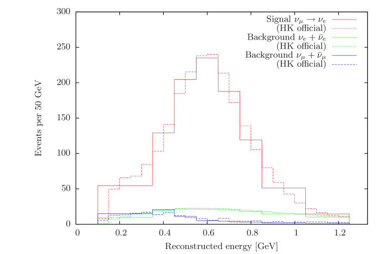
Figure 25: T2HK appearance spectrum from our simulation compared to official event rates [38]. Note that the finer binning of the rates published by T2HK are shown for reference, but this finer granularity is not used in their oscillation fits; the binning we have used in our own fits has been chosen to match that of the official T2HK studies

Appendix B Total number of events for all configurations

In Table 5, we show the expected total rates for events and backgrounds for all configurations, discussed in this work. We adopt the true values according to NuFit 2.2, shown in Tab. 2, but assume $\delta=0$. Two mass orderings are considered. For all cases, cumulative run time is set 10 years. For DUNE, we take events from 0.5 GeV to 8 GeV, while for the other configurations we take from 0.1 GeV to 1.2 GeV.

	$\nu_{\mu}\to\nu_{e}$		$\nu_{\mu}\to\nu_{\mu}$		$\overline{\nu}_{\mu}\to\overline{\nu}_{e}$		$\overline{\nu}_{\mu}\to\overline{\nu}_{\mu}$
	NO	IO	NO	IO	NO	IO	NO	IO
2-horn DUNE (total)	2353	1589	13269	13189	667	1210	13180	13095
2-horn DUNE (BG)	486	502	200	203	253	252	111	112
3-horn DUNE (total)	2317	1561	13773	13774	587	1087	5125	5081
3-horn DUNE (BG)	488	504	199	203	228	227	90	92
nuPIL DUNE (total)	1209	721	5756	5801	230	580	2079	2077
nuPIL DUNE (BG)	111	116	84	85	43	42	38	38
staged T2HK (total)	2294	2514	9221	9157	2093	2715	10997	10855
staged T2HK (BG)	522	525	619	619	695	694	805	805
1tank T2HK (total)	1638	1795	6587	6540	1495	1939	7855	7754
1tank T2HK (BG)	373	375	442	442	496	495	575	575
T2HKK$1.5^{\circ}$ (total)	207	196	3151	3066	288	275	4453	4362
T2HKK$1.5^{\circ}$ (BG)	96	96	117	117	148	148	176	176
T2HKK$2.0^{\circ}$ (total)	163	154	1913	1854	198	194	2331	2256
T2HKK$2.0^{\circ}$ (BG)	51	51	53	53	71	71	63	63
T2HKK$2.5^{\circ}$ (total)	121	116	1269	1283	135	146	1322	1328
T2HKK$2.5^{\circ}$ (BG)	29	29	36	36	37	37	41	41

Table 5: The total rate of events and backgrounds for all configurations with cumulative run time of 10 years, assuming $\delta=0$ for normal ordering (NO) and inverse ordering (IO). The true values are adopted according to the best of NuFit 2.2, shown in Tab. 2. For all configurations of DUNE, we take events from 0.5 GeV to 8 GeV, while for the others we take from 0.1 GeV to 1.2 GeV.

Appendix C Mass ordering sensitivity at high significance

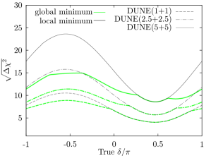
Figure 26: Left: Comparison of our reported sensitivities based on the global minimum and more common published versions which show only a local minimum. This is due to the presence of additional wrong-ordering minima at high significance in the global data. Right: The prior on $\Delta m^{2}_{21}$ provided by the NuFit global fit [46]. Additional local minima with significances around $5\sigma$ ($\Delta m^{2}_{21}\approx 1.6\times 10^{-4}$ eV²) and $10\sigma$ ($\Delta m^{2}_{21}\approx 2.6\times 10^{-4}$ eV²) lead to the unusual behaviour in our reported mass ordering sensitivities.

The sensitivity to mass ordering is conventionally reported as the difference between the value of a $\chi^{2}$ statistic for the true parameter set and the close degenerate set with the atmospheric mass splitting changed by the following mapping,

$$\Delta m^{2}_{31}\to-\Delta m^{2}_{31}+\Delta m^{2}_{21}.$$

This local minimum becomes a worse and worse fit as data is collected, and reaches a $\Delta\chi^{2}$ value of above $8\sigma$ within a few years of running DUNE. This method computes the decreasing quality of a poor fit to the data; however, there are lots of parameter sets which are poor fits to the current data, and many cannot be excluded with a significance greater than $8\sigma$. Statistically speaking, to establish the mass ordering we must exclude all possible parameter sets with that ordering regardless of the other parameter values. In some circumstances, this may mean the local minimum identified above is not the true global wrong-ordering minimum. We find this problem is relevant for DUNE as soon as the local minimum approaches a $5\sigma$ exclusion. This is because the global prior for the solar mass-squared splitting, $\Delta m^{2}_{21}$ has a second minimum at around this significance. The long-baseline experiments considered in this paper, offer no sensitivity to this parameter themselves, and rely on the priors to help constrain it. We have plotted the prior that we have used in our simulations in Fig. 26, where the second minimum can be seen just above the global minimum. For DUNE to exclude the wrong mass ordering at above $5\sigma$, we must ensure it considers all values of $\Delta m^{2}_{21}$ allowed by the global data at this significance. We find that DUNE can often exclude this minimum only at lower significance than the more obvious local minimum corresponding to the expected degeneracy. This causes the lower significances, and discontinuous behaviour, that we have reported in Section 4.1. On average, this reduces the expected significance of the mass ordering measurement by around $5\sigma$.

Of course, predicting any sensitivities at high significance requires good control over all other aspects of the statistical modelling, and we do not pretend that our method correctly models all uncertainties up to very small fluctuations. However, we point out this particular subtlety as a concrete example of how the oft quoted sensitivity is not quite what it seems: it is the confidence at which we can expect to exclude a particular local minimum, not to the best-fitting set of parameters with the wrong ordering. The difference in these quantities starts to become relevant at for DUNE at very modest exposures. In the left panel of Fig. 26, we show the difference in $\Delta\chi^{2}$ values for the local minimum and the full set of wrong ordering parameter sets (green), which starts to be visible after only $2$ years run time. We hope that this example helps to highlight some of the complexities of making precise statements with high confidence sensitivities.

References

- Abe et al. [2011] K. Abe et al. (T2K Collaboration), Phys.Rev.Lett. 107, 041801 (2011), arXiv:1106.2822 [hep-ex] .
- An et al. [2012] F. An et al. (DAYA-BAY Collaboration), Phys.Rev.Lett. 108, 171803 (2012), arXiv:1203.1669 [hep-ex] .
- Ahn et al. [2012] J. Ahn et al. (RENO collaboration), Phys.Rev.Lett. 108, 191802 (2012), arXiv:1204.0626 [hep-ex] .
- An et al. [2013] F. An et al. (Daya Bay), Chin.Phys. C37, 011001 (2013), arXiv:1210.6327 [hep-ex] .
- Aguilar-Arevalo et al. [2009] A. A. Aguilar-Arevalo et al. (MiniBooNE), Phys. Rev. Lett. 102, 101802 (2009), arXiv:0812.2243 [hep-ex] .
- Aguilar-Arevalo et al. [2013] A. A. Aguilar-Arevalo et al. (MiniBooNE), Phys. Rev. Lett. 110, 161801 (2013), arXiv:1207.4809 [hep-ex] .
- Aguilar-Arevalo et al. [2001] A. Aguilar-Arevalo et al. (LSND), Phys. Rev. D64, 112007 (2001), arXiv:hep-ex/0104049 [hep-ex] .
- Ballett et al. [2016] P. Ballett, S. F. King, S. Pascoli, N. W. Prouse, and T. Wang, (2016), arXiv:1612.01999 [hep-ph] .
- Ma [2016] E. Ma, Phys. Lett. B755, 348 (2016), arXiv:1601.00138 [hep-ph] .
- Lu and Ding [2016] J.-N. Lu and G.-J. Ding, (2016), arXiv:1610.05682 [hep-ph] .
- Berryman and Hernández [2016] J. M. Berryman and D. Hernández, (2016), arXiv:1611.07033 [hep-ph] .
- Antonello et al. [2015] M. Antonello et al. (LAr1-ND, ICARUS-WA104, MicroBooNE), (2015), arXiv:1503.01520 [physics.ins-det] .
- An et al. [2016] F. An et al. (JUNO), J. Phys. G43, 030401 (2016), arXiv:1507.05613 [physics.ins-det] .
- Djurcic et al. [2015] Z. Djurcic et al. (JUNO), (2015), arXiv:1508.07166 [physics.ins-det] .
- Kim [2015] S.-B. Kim, Proceedings, Neutrino Oscillation Workshop (NOW 2014): Conca Specchiulla, Otranto, Lecce, Italy, September 7-14, 2014, Nucl. Part. Phys. Proc. 265-266, 93 (2015), arXiv:1412.2199 [hep-ex] .
- Adamson et al. [2016a] P. Adamson et al. (NOvA), Phys. Rev. Lett. 116, 151806 (2016a), arXiv:1601.05022 [hep-ex] .
- Adamson et al. [2016b] P. Adamson et al. (NOvA), Phys. Rev. D93, 051104 (2016b), arXiv:1601.05037 [hep-ex] .
- Abe et al. [2015] K. Abe et al. (T2K), Phys. Rev. D91, 072010 (2015), arXiv:1502.01550 [hep-ex] .
- Abe et al. [2014] K. Abe et al. (Hyper-Kamiokande Working Group) (2014) arXiv:1412.4673 [physics.ins-det] .
- Adams et al. [2013] C. Adams et al. (LBNE Collaboration), (2013), arXiv:1307.7335 [hep-ex] .
- Acciarri et al. [2015] R. Acciarri et al. (DUNE), (2015), arXiv:1512.06148 [physics.ins-det] .
- Fukuda et al. [2003] Y. Fukuda et al. (Super-Kamiokande Collaboration), Nucl.Instrum.Meth. A501, 418 (2003).
- Soumya et al. [2016] C. Soumya, K. N. Deepthi, and R. Mohanta, Adv. High Energy Phys. 2016, 9139402 (2016), arXiv:1408.6071 [hep-ph] .
- Coloma et al. [2013] P. Coloma, P. Huber, J. Kopp, and W. Winter, Phys.Rev. D87, 033004 (2013), arXiv:1209.5973 [hep-ph] .
- Ghosh et al. [2016] M. Ghosh, S. Goswami, and S. K. Raut, Eur. Phys. J. C76, 114 (2016), arXiv:1412.1744 [hep-ph] .
- De Romeri et al. [2016] V. De Romeri, E. Fernandez-Martinez, and M. Sorel, (2016), arXiv:1607.00293 [hep-ph] .
- Nath et al. [2016] N. Nath, M. Ghosh, and S. Goswami, Nucl. Phys. B913, 381 (2016), arXiv:1511.07496 [hep-ph] .
- Barger et al. [2016] V. Barger, A. Bhattacharya, A. Chatterjee, R. Gandhi, D. Marfatia, and M. Masud, Int. J. Mod. Phys. A31, 1650020 (2016), arXiv:1405.1054 [hep-ph] .
- Barger et al. [2014] V. Barger, A. Bhattacharya, A. Chatterjee, R. Gandhi, D. Marfatia, and M. Masud, Phys. Rev. D89, 011302 (2014), arXiv:1307.2519 [hep-ph] .
- Bora et al. [2015] K. Bora, D. Dutta, and P. Ghoshal, Mod. Phys. Lett. A30, 1550066 (2015), arXiv:1405.7482 [hep-ph] .
- Bishai et al. [2012] M. Bishai, M. V. Diwan, S. Kettell, J. Stewart, B. Viren, E. Worchester, and L. Whitehead, (2012), arXiv:1203.4090 [hep-ex] .
- Agarwalla et al. [2013a] S. Agarwalla et al. (LAGUNA-LBNO Collaboration), (2013a), arXiv:1312.6520 [hep-ph] .
- Ghosh et al. [2014] M. Ghosh, P. Ghoshal, S. Goswami, and S. K. Raut, JHEP 03, 094 (2014), arXiv:1308.5979 [hep-ph] .
- Lagrange et al. [2015] J. B. Lagrange, J. Pasternak, A. Bross, and A. Liu, in 17th International Workshop on Neutrino Factories and Future Neutrino Facilities Search (NuFact15) Rio de Janeiro, Brazil, August 10-15, 2015 (2015).
- Liu et al. [2016] A. Liu, A. Bross, and J.-B. Lagrange, in Proceedings, 7th International Particle Accelerator Conference (IPAC 2016) (2016) p. THPMB055.
- Lagrange et al. [2016] J.-B. Lagrange, J. Pasternak, A. Bross, A. Liu, R. Appleby, and S. Tygier, in Proceedings, 7th International Particle Accelerator Conference (IPAC 2016) (2016) p. THPMB054.
- Choubey et al. [2011] S. Choubey et al. (IDS-NF), (2011), arXiv:1112.2853 [hep-ex] .
- Abe et al. [2016a] K. Abe et al. (Hyper-Kamiokande Proto-Collaboration), “Hyper-Kamiokande Design Report,” (2016a), KEK Preprint 2016-21, ICRR-Report-701-2016-1.
- Abe et al. [2016b] K. Abe et al. (Hyper-Kamiokande Proto-Collaboration), (2016b), arXiv:1611.06118 [hep-ex] .
- Hagiwara et al. [2006] K. Hagiwara, N. Okamura, and K.-i. Senda, Phys. Lett. B637, 266 (2006), [Erratum: Phys. Lett.B641,491(2006)], arXiv:hep-ph/0504061 [hep-ph] .
- Hagiwara et al. [2007] K. Hagiwara, N. Okamura, and K.-i. Senda, Phys. Rev. D76, 093002 (2007), arXiv:hep-ph/0607255 [hep-ph] .
- Kajita et al. [2007] T. Kajita, H. Minakata, S. Nakayama, and H. Nunokawa, Phys. Rev. D75, 013006 (2007), arXiv:hep-ph/0609286 [hep-ph] .
- Ishitsuka et al. [2005] M. Ishitsuka, T. Kajita, H. Minakata, and H. Nunokawa, Phys. Rev. D72, 033003 (2005), arXiv:hep-ph/0504026 [hep-ph] .
- Fukasawa et al. [2016] S. Fukasawa, M. Ghosh, and O. Yasuda, (2016), arXiv:1607.03758 [hep-ph] .
- Beringer et al. [2012] J. Beringer et al. (Particle Data Group), Phys.Rev. D86, 010001 (2012).
- Gonzalez-Garcia et al. [2014] M. C. Gonzalez-Garcia, M. Maltoni, and T. Schwetz, JHEP 11, 052 (2014), arXiv:1409.5439 [hep-ph] .
- Asano and Minakata [2011] K. Asano and H. Minakata, JHEP 1106, 022 (2011), arXiv:1103.4387 .
- Agarwalla et al. [2013b] S. K. Agarwalla, Y. Kao, and T. Takeuchi, (2013b), arXiv:1302.6773 .
- Johnson et al. [2015] M. B. Johnson, E. M. Henley, and L. S. Kisslinger, Phys. Rev. D91, 076005 (2015), arXiv:1501.04093 [hep-ph] .
- Minakata and Parke [2016] H. Minakata and S. J. Parke, JHEP 01, 180 (2016), arXiv:1505.01826 [hep-ph] .
- Denton et al. [2016] P. B. Denton, H. Minakata, and S. J. Parke, JHEP 06, 051 (2016), arXiv:1604.08167 [hep-ph] .
- Agarwalla [2014] S. K. Agarwalla, Adv. High Energy Phys. 2014, 457803 (2014), arXiv:1401.4705 [hep-ph] .
- Huber and Kopp [2011] P. Huber and J. Kopp, JHEP 03, 013 (2011), [Erratum: JHEP05,024(2011)], arXiv:1010.3706 [hep-ph] .
- Geer et al. [2007] S. Geer, O. Mena, and S. Pascoli, Phys. Rev. D75, 093001 (2007), arXiv:hep-ph/0701258 [HEP-PH] .
- Coloma and Fernandez-Martinez [2012] P. Coloma and E. Fernandez-Martinez, JHEP 04, 089 (2012), arXiv:1110.4583 [hep-ph] .
- Agarwalla et al. [2014] S. K. Agarwalla et al. (LAGUNA-LBNO), (2014), arXiv:1412.0593 [hep-ph] .
- Minakata and Parke [2013] H. Minakata and S. J. Parke, Phys. Rev. D87, 113005 (2013), arXiv:1303.6178 [hep-ph] .
- Coloma et al. [2014] P. Coloma, H. Minakata, and S. J. Parke, Phys. Rev. D90, 093003 (2014), arXiv:1406.2551 [hep-ph] .
- Antusch et al. [2007] S. Antusch, P. Huber, S. F. King, and T. Schwetz, JHEP 04, 060 (2007), arXiv:hep-ph/0702286 [HEP-PH] .
- Ballett et al. [2014a] P. Ballett, S. F. King, C. Luhn, S. Pascoli, and M. A. Schmidt, Phys. Rev. D89, 016016 (2014a), arXiv:1308.4314 [hep-ph] .
- Girardi et al. [2015a] I. Girardi, S. T. Petcov, and A. V. Titov, Nucl. Phys. B894, 733 (2015a), arXiv:1410.8056 [hep-ph] .
- Ballett et al. [2014b] P. Ballett, S. F. King, C. Luhn, S. Pascoli, and M. A. Schmidt, JHEP 12, 122 (2014b), arXiv:1410.7573 [hep-ph] .
- Girardi et al. [2015b] I. Girardi, S. T. Petcov, and A. V. Titov, Eur. Phys. J. C75, 345 (2015b), arXiv:1504.00658 [hep-ph] .
- King [2015] S. F. King, J. Phys. G42, 123001 (2015), arXiv:1510.02091 [hep-ph] .
- King [2017] S. F. King, Prog. Part. Nucl. Phys. 94, 217 (2017), arXiv:1701.04413 [hep-ph] .
- Coloma et al. [2012] P. Coloma, A. Donini, E. Fernandez-Martinez, and P. Hernandez, JHEP 06, 073 (2012), arXiv:1203.5651 [hep-ph] .
- Huber et al. [2005] P. Huber, M. Lindner, and W. Winter, Comput. Phys. Commun. 167, 195 (2005), arXiv:hep-ph/0407333 [hep-ph] .
- Huber et al. [2007] P. Huber, J. Kopp, M. Lindner, M. Rolinec, and W. Winter, Comput. Phys. Commun. 177, 432 (2007), arXiv:hep-ph/0701187 [hep-ph] .
- Alion et al. [2016] T. Alion et al. (DUNE), (2016), arXiv:1606.09550 [physics.ins-det] .
- Papadimitriou et al. [2016] V. Papadimitriou et al., in Proceedings, 7th International Particle Accelerator Conference (IPAC 2016) (2016) p. TUPMR025.
- DUNE Collaboration [2016a] DUNE Collaboration, (2016a), http://home.fnal.gov/ljf26/DUNEFluxes/.
- DUNE Collaboration [2016b] DUNE Collaboration, (2016b), https://indico.fnal.gov/conferenceDisplay.py?confId=12361.
- Acciarri et al. [2016] R. Acciarri et al. (DUNE), (2016), arXiv:1601.05471 [physics.ins-det] .
- Koseki [2015] T. Koseki, “J-PARC Accelerator: achievement and future upgrade,” (2015), Talk presented at the Workshop for Neutrino Programs with Facilities in Japan, August 4, 2015 Tokai, Japan.
- Kobayashi [2015] T. Kobayashi, “Potential J-PARC beam power improvement and beam delivery before 2026,” (2015), Talk presented at the Workshop for Neutrino Programs with Facilities in Japan, August 4, 2015, Tokai, Japan.
- Shiozawa [2016] M. Shiozawa, “Hyper-Kamiokande,” (2016), Talk presented at the Third International Meeting for Large Neutrino Infrastructures, May 30, 2016, Tsukuba, Japan.
- Huber et al. [2002] P. Huber, M. Lindner, and W. Winter, Nucl. Phys. B645, 3 (2002), hep-ph/0204352 .
- Andreopoulos et al. [2010] C. Andreopoulos et al., Nucl. Instrum. Meth. A614, 87 (2010), arXiv:0905.2517 [hep-ph] .
- Forero et al. [2014] D. V. Forero, M. Tortola, and J. W. F. Valle, Phys. Rev. D90, 093006 (2014), arXiv:1405.7540 [hep-ph] .
- Capozzi et al. [2016] F. Capozzi, E. Lisi, A. Marrone, D. Montanino, and A. Palazzo, Nucl. Phys. B908, 218 (2016), arXiv:1601.07777 [hep-ph] .
- Qian et al. [2012] X. Qian, A. Tan, W. Wang, J. J. Ling, R. D. McKeown, and C. Zhang, Phys. Rev. D86, 113011 (2012), arXiv:1210.3651 [hep-ph] .
- Ciuffoli et al. [2014] E. Ciuffoli, J. Evslin, and X. Zhang, JHEP 01, 095 (2014), arXiv:1305.5150 [hep-ph] .
- Blennow et al. [2014] M. Blennow, P. Coloma, P. Huber, and T. Schwetz, JHEP 03, 028 (2014), arXiv:1311.1822 [hep-ph] .
- Elevant and Schwetz [2015] J. Elevant and T. Schwetz, JHEP 09, 016 (2015), arXiv:1506.07685 [hep-ph] .
- Blennow et al. [2015] M. Blennow, P. Coloma, and E. Fernandez-Martinez, JHEP 03, 005 (2015), arXiv:1407.3274 [hep-ph] .