Geometric convergence bounds for Markov chains in Wasserstein distance based on generalized drift and contraction conditions

Abstract

Let $(X_{n})_{n=0}^{\infty}$ denote a Markov chain on a Polish space that has a stationary distribution $\varpi$. This article concerns upper bounds on the Wasserstein distance between the distribution of $X_{n}$ and $\varpi$. In particular, an explicit geometric bound on the distance to stationarity is derived using generalized drift and contraction conditions whose parameters vary across the state space. These new types of drift and contraction allow for sharper convergence bounds than the standard versions, whose parameters are constant. Application of the result is illustrated in the context of a non-linear autoregressive process and a Gibbs algorithm for a random effects model.

1 Introduction

The study of convergence to stationarity of Markov chains commonly requires the specification of a metric on an appropriate space of probability distributions. The standard has long been total variation (TV) distance, but, over the last decade or so, Wasserstein distance has received a good deal of attention as well. One obvious reason for studying convergence in Wasserstein distance is that there exist Markov chains that do not actually converge in TV distance, but do converge in some Wasserstein distance (see, e.g., Hairer et al., 2011; Butkovsky, 2014). Another, perhaps more important, reason stems from the current focus on so-called big data problems, which leads to the study of Markov chains on high-dimensional state spaces. Indeed, it is becoming clear that the techniques used for developing Wasserstein bounds are more robust to increasing dimension than are those used to construct TV bounds (see, e.g., Hairer et al., 2011, 2014; Durmus and Moulines, 2015; Eberle et al., 2019; Qin and Hobert, 2021+). In this paper, we study convergence rates of Markov chains with respect to Wasserstein distances. In particular, we develop explicit geometric (exponential) convergence bounds using generalized (or localized) versions of the usual drift and contraction conditions.

Previous work devoted to convergence analysis of Markov chains with respect to Wasserstein distances includes Jarner and Tweedie (2001), Hairer et al. (2011), Butkovsky (2014), Durmus and Moulines (2015), and Douc et al. (2018). A recurring theme in these papers is the combination of drift and contraction. The basic program is to first establish a strong contraction condition on a coupling set (which is a subset of ${\mathsf{X}}\times{\mathsf{X}}$, where ${\mathsf{X}}$ is the state space), and then to use a Lyapunov drift condition to drive a coupled version of the Markov chain towards that subset. The goal of this article is to provide a more refined version of this program, where instead of considering only two sets of points in ${\mathsf{X}}\times{\mathsf{X}}$, i.e., the coupling set and its complement, one takes into account the localized behavior of the Markov chain at each point of the product state space. Indeed, we demonstrate that geometric convergence bounds can be constructed using a generalized version of drift and contraction, which we now describe.

When developing drift and contraction conditions for specific problems, the parameters in these inequalities are often initially non-constant. The varying parameters may encode rich information about the dynamics of the chain. The usual drift and contraction conditions (with constant parameters) are typically obtained by taking the supremum over the coupling set, and again over the compliment of the coupling set. Naturally, this process can result in a substantial loss of information. The bounds that we provide can be constructed directly from the drift and contraction conditions with non-constant parameters — the generalized drift and contraction conditions. This procedure does not require selecting a coupling set, and can potentially lead to sharper bounds based on weaker assumptions, compared to previous results. For example, our upper bound on the geometric convergence rate is always better (i.e., smaller) than that in Durmus and Moulines (2015). Our work draws inspiration from the “small function” version of the minorization condition (see, e.g., Nummelin, 1984, Section 2.3), which can be considered a generalized version of the usual minorization condition (with constant parameter). The local contractive behavior of a Markov chain considered in Steinsaltz (1999) and Eberle and Majka (2019) is also related to the generalized conditions that we use.

The rest of the article is organized as follows. In Section 2, after setting notation, we give a detailed account of generalized drift and contraction conditions. We construct a geometric convergence bound based on these conditions, and compare it to bounds based on standard drift and contraction. The proofs are postponed to Section 3. In Section 4, we use a perturbed autoregressive process and a Gibbs algorithm for a random effects model to demonstrate how our results can be applied. These applications provide concrete examples of the extent to which the new bound improves upon standard ones. Finally, Appendix A contains a rigorous comparison of the bounds developed herein with those of Durmus and Moulines (2015), and Appendix B contains some technical details supporting the analysis in Section 4.

2 Generalized Drift and Contraction

Let $({\mathsf{X}},\varrho)$ be a complete separable metric space (i.e., Polish metric space), and assume that $\mathcal{B}$ is the associated Borel $\sigma$-algebra. Let $\mathcal{P}({\mathsf{X}})$ denote the set of probability measures on $({\mathsf{X}},\mathcal{B})$, and let $\delta_{x}$ denote the point mass (or Dirac measure) at $x$. For $\mu,\nu\in\mathcal{P}({\mathsf{X}})$, let

$$\mathcal{C}(\mu,\nu)=\big{\{}\upsilon\in\mathcal{P}({\mathsf{X}}\times{\mathsf{X}}):\;\upsilon(A_{1}\times{\mathsf{X}})=\mu(A_{1})\,,\;\upsilon({\mathsf{X}}\times A_{2})=\nu(A_{2})\text{ for all }A_{1},A_{2}\in\mathcal{B}\big{\}}\,.$$

This is the set of couplings of $\mu$ and $\nu$. Let $\psi:{\mathsf{X}}\times{\mathsf{X}}\to[0,\infty)$ be a lower semi-continuous function. This function will be referred to as a cost function, and is usually taken to be a distance-like function that is vanishing if and only if its two arguments coincide. The Wasserstein divergence between $\mu\in\mathcal{P}({\mathsf{X}})$ and $\nu\in\mathcal{P}({\mathsf{X}})$ induced by $\psi$ is defined to be

$$W_{\psi}(\mu,\nu)=\inf_{\upsilon\in\mathcal{C}(\mu,\nu)}\int_{{\mathsf{X}}\times{\mathsf{X}}}\psi(x,y)\upsilon(\mathrm{d}x,\mathrm{d}y)\,.$$

Taking $\psi=\varrho$ gives the $L_{1}$-Wasserstein (or Kantorovich-Rubinstein) distance induced by $\varrho$. In fact, for $p\geq 1$, one can define

$$\mathcal{P}_{\varrho,p}({\mathsf{X}})=\left\{\mu\in\mathcal{P}({\mathsf{X}})\,:\;\int_{{\mathsf{X}}}\varrho(x,y)^{p}\,\mu(\mathrm{d}y)<\infty\text{ for some }x\in{\mathsf{X}}\right\},$$

and let

$$W_{\varrho,p}(\mu,\nu)=\left(\inf_{\upsilon\in\mathcal{C}(\mu,\nu)}\int_{{\mathsf{X}}\times{\mathsf{X}}}\varrho(x,y)^{p}\,\upsilon(\mathrm{d}x,\mathrm{d}y)\right)^{1/p}.$$

Then $W_{\varrho,p}$ is the $L_{p}$-Wasserstein distance, and $(\mathcal{P}_{\varrho,p}({\mathsf{X}}),W_{\varrho,p})$ forms a Polish metric space (see, e.g., Villani, 2009, Theorem 6.18).

Let $P:{\mathsf{X}}\times\mathcal{B}\to[0,1]$ be a Markov transition kernel (Mtk), and for a positive integer $n$, let $P^{n}:{\mathsf{X}}\times\mathcal{B}\to[0,1]$ be the corresponding $n$-step Mtk. (As usual, we write $P$ instead of $P^{1}$.) Let $P^{0}$ be the identity kernel, i.e., $P^{0}(x,A)=1_{x\in A}$ for $A\in\mathcal{B}$. For $\mu\in\mathcal{P}({\mathsf{X}})$ and a measurable function $f:{\mathsf{X}}\to\mathbb{R}$, let $\mu f=\int_{{\mathsf{X}}}f(x)\mu(\mathrm{d}x)$, $\mu P^{n}(\cdot)=\int_{{\mathsf{X}}}P^{n}(x,\cdot)\mu(\mathrm{d}x)$, and $P^{n}f(\cdot)=\int_{{\mathsf{X}}}f(x)P^{n}(\cdot,\mathrm{d}x)$ (assuming the integrals are well-defined).

Our goal is to establish new conditions under which the Markov chain defined by $P$ converges in $W_{\psi}$ to a limiting distribution $\varpi\in\mathcal{P}({\mathsf{X}})$ at a geometric rate. More specifically, based on these new conditions, we will construct convergence bounds of the form

$$W_{\psi}(\delta_{x}P^{n},\varpi)\leq c_{x}\,\rho^{n}\,,$$

where $x\in{\mathsf{X}}$, $n\in\{0,1,2,\dots\}=:\mathbb{Z}_{+}$, $c_{x}<\infty$, and $\rho<1$. Moreover, we will provide explicit formulas for $c_{x}$ and $\rho$. $\rho$ is an upper bound on the geometric convergence rate of the chain, defined as

$$\exp\left(\sup_{x\in{\mathsf{X}}}\limsup_{n\to\infty}\frac{\log W_{\psi}(\delta_{x}^{n},\varpi)}{n}\right)$$

(see Roberts and Tweedie, 2001, page 40). We will be particularly interested in finding smaller values of $\rho$ compared to existing bounds in the literature.

We first review a set of standard drift and contraction conditions that can be used to produce this type of bound.

1. There exist a measurable function $V:{\mathsf{X}}\to[0,\infty)$ and $a\in[0,\infty)$ such that

   $$\psi(x,y)\leq a[V(x)+V(y)+1]\,,\quad(x,y)\in{\mathsf{X}}\times{\mathsf{X}}\,,$$ (1)

   and there exist $\eta\in[0,1)$ and $L\in[0,\infty)$ such that

   $$PV(x)\leq\eta V(x)+L\,,\quad x\in{\mathsf{X}}\,.$$ (2)

2. There exist $\gamma\in[0,1)$ and $K\in[0,\infty)$ such that for each $(x,y)\in{\mathsf{X}}\times{\mathsf{X}}$,

   $$W_{\psi}(\delta_{x}P,\delta_{y}P)\leq\begin{cases}\gamma\psi(x,y)\,,&(x,y)\in C\,,\\ K\psi(x,y)\,,&(x,y)\not\in C\,,\end{cases}$$

   where the coupling set $C$ is defined to be $\big{\{}(x,y)\in{\mathsf{X}}\times{\mathsf{X}}:V(x)+V(y)<d\big{\}}$, with $d>2L/(1-\eta)$.

Condition $(A2)$, referred to as a contraction condition, partitions the product state space ${\mathsf{X}}\times{\mathsf{X}}$ into two regions, $C$ and its complement. The coupling set $C$ is a “good” set, where two coupled copies of the Markov chain tend to approach each other. Condition $(A1)$, referred to as a drift condition, is a classical assumption that drives the coupled chains towards $C$. Taking into account the magnitude of contraction and drift (quantified by parameters such as $\gamma$, $L$, and $K$), it’s possible to construct a quantitative convergence bound. The following is an example of this.

Corollary 2.1.

Suppose that $(A1)$, $(A2)$, and the following condition all hold:

1. Either $K\leq 1$ or

   $$\log K\log(2L+1)<\log\frac{1}{\gamma}\log\frac{d+1}{\eta d+2L+1}\,.$$ (3)

Then, for each $\mu,\nu\in\mathcal{P}({\mathsf{X}})$ and real number $r$ such that

$$\frac{\log(2L+1)}{\log(2L+1)+\log(1/\gamma)}<r<\frac{\log[(d+1)/(\eta d+2L+1)]}{\log(K\vee 1)+\log[(d+1)/(\eta d+2L+1)]}\,,$$ (4)

we have

$$W_{\psi}(\mu P^{n},\nu P^{n})\leq a(\mu V+\nu V+1)\rho_{r}^{n}\,,\quad n\in\mathbb{Z}_{+},$$

where

$$\rho_{r}=\left[\gamma^{r}(2L+1)^{1-r}\right]\vee\left[K^{r}\left(\frac{\eta d+2L+1}{d+1}\right)^{1-r}\right]<1\,.$$

In particular, if $P$ admits a stationary distribution $\varpi$, then for $\mu\in\mathcal{P}({\mathsf{X}})$,

$$W_{\psi}(\mu P^{n},\varpi)\leq a\left(\mu V+\frac{L}{1-\eta}+1\right)\rho_{r}^{n}\,,\quad n\in\mathbb{Z}_{+}.$$

Remark 2.2.

The fact that $d>2L/(1-\eta)$ implies that $(\eta d+2L+1)/(d+1)<1$, and it follows that

$$0\leq\frac{\log(2L+1)}{\log(2L+1)+\log(1/\gamma)}<\frac{\log[(d+1)/(\eta d+2L+1)]}{\log(K\vee 1)+\log[(d+1)/(\eta d+2L+1)]}\leq 1$$

whenever $K\leq 1$ or (3) is satisfied. Thus, (4) makes sense, and $r\in(0,1)$.

Remark 2.3.

We provide conditions for the existence and uniqueness of stationary distributions in a more general context in Propositions 2.9 and 2.10. Based on these propositions, one can check that, if $(A1)$-$(A3)$ hold and $\psi=\varrho$, then $P$ admits a unique stationary distribution $\varpi$.

Remark 2.4.

One can use Proposition 2.9 to derive the following alternative convergence bound when $(A1)$-$(A3)$ hold and $\psi=\varrho$. For $x\in{\mathsf{X}}$ and $r$ satisfying (4),

$$W_{\varrho}(\delta_{x}P^{n},\varpi)\leq a\frac{(\eta+1)V(x)+L+1}{1-\rho_{r}}\rho_{r}^{n}\,,\quad n\in\mathbb{Z}_{+}\,,$$

where $\rho_{r}\in[0,1)$ is given in Corollary 2.1. However, this bound is slightly looser than the one in Corollary 2.1.

Corollary 2.1 can be derived using the main theorem of this article, which will soon be stated. Results similar to Corollary 2.1 have been derived in various contexts; see, e.g., Butkovsky (2014) and Durmus and Moulines (2015). The most recent account is Theorem 20.4.5 of Douc et al. (2018), where the authors establish geometric convergence under a condition akin to $(A1)$ along with $(A2)$ with $K\leq 1$. Douc et al.’s (2018) Theorem 20.4.5 does not provide a fully explicit convergence bound, although it is possible to derive such a bound based on the proof of said result, and it will resemble what is given in Corollary 2.1. A fully computable geometric convergence bound is given in Durmus and Moulines (2015) for the case that $\psi=\varrho$, $\varrho$ is bounded, and $K\leq 1$. The bound therein is similar to what is given in Corollary 2.1, albeit slightly looser, as shown in Section A of the Appendix.

One can also derive the following continuous version of Corollary 2.1, whose proof will be given in Section 3.

Corollary 2.5.

Let $(P^{t})_{t\geq 0}$ be a Markov semigroup on $({\mathsf{X}},\mathcal{B})$. Suppose that there exists $t_{*}>0$ such that $P^{t_{*}}$ (in place of $P$) satisfies $(A1)$-$(A3)$, and that $P^{t_{*}}$ admits a unique stationary distribution $\varpi$. Suppose further that there exists $b<\infty$ such that for every $(x,y)\in{\mathsf{X}}\times{\mathsf{X}}$ and $t\in[0,t_{*})$,

$$W_{\psi}(\delta_{x}P^{t},\delta_{y}P^{t})\leq b\psi(x,y)\;.$$ (5)

Then $\varpi$ is also the unique stationary distribution of $(P^{t})_{t}$. Moreover, for $\mu\in\mathcal{P}({\mathsf{X}})$ and $t\geq 0$,

$$W_{\psi}(\mu P^{t},\varpi)\leq ab\left(\mu V+\frac{L}{1-\eta}+1\right)\rho_{r}^{\lfloor t/t_{*}\rfloor}\;,$$

where $\lfloor\cdot\rfloor$ returns the largest integer that does not exceed its argument, $r$ satisfies (4), and $\rho_{r}\in[0,1)$ is defined as in Corollary 2.1.

Looking back at Condition $(A2)$, a natural question that can be raised is, whether a more delicate analysis is possible if one divides the product space ${\mathsf{X}}\times{\mathsf{X}}$ into more than two parts. To be precise, instead of categorizing the behavior of $W_{\psi}(\delta_{x}P,\delta_{y}P)$ into two cases, can one gain more by taking into account the local behavior of $W_{\psi}(\delta_{x}P,\delta_{y}P)$ for each value of $(x,y)$? This prompts us to study the convergence properties of a Markov chain under the following generalized versions of $(A1)$ and $(A2)$.

1. There exists a measurable function $V:{\mathsf{X}}\to[0,\infty)$ and $a\in[0,\infty)$ such that

   $$\psi(x,y)\leq a[V(x)+V(y)+1]\,,\quad(x,y)\in{\mathsf{X}}\times{\mathsf{X}}\,,$$

   and $PV(x)<\infty$ for each $x\in{\mathsf{X}}$.

2. There exists a measurable function $\Gamma:{\mathsf{X}}\times{\mathsf{X}}\to[0,\infty)$ such that for each $(x,y)\in{\mathsf{X}}\times{\mathsf{X}}$,

   $$W_{\psi}(\delta_{x}P,\delta_{y}P)\leq\Gamma(x,y)\,\psi(x,y)\,.$$

The relationship between the two conditions above and their standard counterparts is quite obvious. In particular, $(A2)$ is just $(B2)$ when $\Gamma$ is constant over some coupling set $C$ as well as over its complement, assuming that $\Gamma(x,y)<1$ when $(x,y)\in C$. $(B2)$, while being weaker than $(A2)$, may also incorporate information on the localized contractive behavior of $P$ that $(A2)$ ignores (depending on how $\Gamma$ is constructed).

Combining $(B1)$ and $(B2)$ with an analog of $(A3)$ that regulates the relationship between $\Gamma(x,y)$ and $(PV(x),PV(y))$ yields our main theorem, which we now state.

Theorem 2.6.

Assume that $(B1)$ and $(B2)$ hold. Let $\Lambda:{\mathsf{X}}\times{\mathsf{X}}\to[0,\infty)$ be such that

$$\Lambda(x,y)\geq\frac{PV(x)+PV(y)+1}{V(x)+V(y)+1}\,.$$

Assume further that the following condition holds:

1. There exists $r\in(0,1)$ such that

   $$\sup_{(x,y)\in{\mathsf{X}}\times{\mathsf{X}}}\Gamma(x,y)^{r}\Lambda(x,y)^{1-r}<1\,.$$ (5)

Then, for $\mu,\nu\in\mathcal{P}({\mathsf{X}})$,

$$W_{\psi}(\mu P^{n},\nu P^{n})\leq a(\mu V+\nu V+1)\rho_{r}^{n}\,,\quad n\in\mathbb{Z}_{+}\,,$$

where $\rho_{r}=\sup_{(x,y)\in{\mathsf{X}}\times{\mathsf{X}}}\Gamma(x,y)^{r}\Lambda(x,y)^{1-r}<1$. In particular, if $P$ admits a stationary distribution $\varpi$, then

$$W_{\psi}(\mu P^{n},\varpi)\leq a(\mu V+\varpi V+1)\rho_{r}^{n}\,,\quad n\in\mathbb{Z}_{+}\,.$$ (6)

Remark 2.7.

It can be shown that $(B3)$ holds whenever

$$\sup_{(x,y)\in{\mathsf{X}}\times{\mathsf{X}}}[\Gamma(x,y)\wedge\Lambda(x,y)]<1\,,$$

and

$$\left(\sup_{x,y:\,\Lambda(x,y)>\Gamma(x,y)}\frac{\log\Lambda(x,y)}{\log\Lambda(x,y)-\log\Gamma(x,y)}\right)\vee 0<\left(\inf_{x,y:\,\Lambda(x,y)<\Gamma(x,y)}\frac{\log\Lambda(x,y)}{\log\Lambda(x,y)-\log\Gamma(x,y)}\right)\wedge 1\,.$$

In this case, $\rho_{r}<1$ whenever

$$\left(\sup_{x,y:\,\Lambda(x,y)>\Gamma(x,y)}\frac{\log\Lambda(x,y)}{\log\Lambda(x,y)-\log\Gamma(x,y)}\right)\vee 0<r<\left(\inf_{x,y:\,\Lambda(x,y)<\Gamma(x,y)}\frac{\log\Lambda(x,y)}{\log\Lambda(x,y)-\log\Gamma(x,y)}\right)\wedge 1\,.$$

Remark 2.8.

The bound in (6) is nontrivial only if $\varpi V<\infty$. This holds under $(A1)$. Indeed, under $(A1)$, $\varpi V\leq L/(1-\eta)$ (Hairer, 2018, Proposition 4.24). If $\psi$ satisfies additional conditions, e.g., $\psi=\varrho$, then an alternative bound holds without the assumption $\varpi V<\infty$. See Propositions 2.9 and 2.10.

The next two propositions give conditions for the existence and uniqueness of stationary distributions.

Proposition 2.9.

Suppose that $(B1)$-$(B3)$ are satisfied, and that the following also holds:

1. There exists $p\in[1,\infty)$ such that

   $$\varrho(x,y)^{p}\leq\psi(x,y),\quad(x,y)\in{\mathsf{X}}\times{\mathsf{X}}.$$

Then there exists $\varpi\in\mathcal{P}_{\varrho,p}({\mathsf{X}})$ and $r\in(0,1)$ such that, for $x\in{\mathsf{X}}$,

$$W_{\varrho,p}(\delta_{x}P^{n},\varpi)\leq a^{1/p}[PV(x)+V(x)+1]^{1/p}\frac{\rho_{r}^{n/p}}{1-\rho_{r}^{1/p}}\,,\quad n\in\mathbb{Z}_{+}\,,$$ (7)

where $\rho_{r}\in[0,1)$ is given in Theorem 2.6. Moreover, $P$ admits at most one stationary distribution.

The condition (B4) has been used previously as a condition to guarantee the existence of a limiting distribution (Douc et al., 2018, Theorem 20.2.1). It may be difficult for $(B4)$ to hold when $\varrho$ is unbounded. To circumvent this, one can replace $\varrho$ with a bounded metric that is topologically equivalent, such as $\varrho\wedge 1$, in the initial setup of the Polish metric space.

Let $C_{b}({\mathsf{X}})$ be the set of bounded, continuous real-valued functions on ${\mathsf{X}}$. We say that $P$ is Feller if $Pf\in C_{b}({\mathsf{X}})$ for each $f\in C_{b}({\mathsf{X}})$.

Proposition 2.10.

Suppose that $(B1)$-$(B4)$ hold. Suppose further that either of the following conditions holds.

1. There exists $K^{\prime}<\infty$ such that, for $(x,y)\in{\mathsf{X}}\times{\mathsf{X}}$, $W_{\varrho}(\delta_{x}P,\delta_{y}P)\leq K^{\prime}\varrho(x,y)$.

2. $P$ is Feller.

Then $\varpi$, as defined in Proposition 2.9, is the unique stationary distribution of $P$.

Remark 2.11.

Note that if $(B2)$ holds with a bounded function $\Gamma$ and $\psi=\varrho$, then $(B4)$ and $(B5)$ hold.

Before going on to the next section, which contains the proofs of Theorem 2.6 and subsequent propositions, we compare Theorem 2.6 with Corollary 2.1, a result based on standard versions of drift and contraction. As we will demonstrate in Section 3, the latter is essentially an application of the former when $\Lambda$ and $\Gamma$ are constant over a coupling set, $C$, as well as over its complement, $({\mathsf{X}}\times{\mathsf{X}})\setminus C$. To make a comparison between the two results, consider the following scenario. Suppose that $P$ satisfies $(A1)$ with a drift function $V:{\mathsf{X}}\to[0,\infty)$, $a\in[0,\infty)$, $\eta\in[0,1)$, and $L\in[0,\infty)$. Then $P$ satisfies $(B1)$ with the same $V$ and $a$. Suppose that $P$ also satisfies $(B2)$ with $\Gamma:{\mathsf{X}}\times{\mathsf{X}}\to[0,\infty)$. Let

$$\Lambda(x,y)=\frac{\eta V(x)+\eta V(y)+2L+1}{V(x)+V(y)+1}\geq\frac{PV(x)+PV(y)+1}{V(x)+V(y)+1}$$

for $(x,y)\in{\mathsf{X}}\times{\mathsf{X}}$. Assume further that $(B3)$ holds and that $P$ has a stationary distribution $\varpi$. We know from Remark 2.8 that $\varpi V<\infty$. In accordance with Theorem 2.6, for $r\in(0,1)$, let

$$\rho_{r}^{B}=\sup_{(x,y)\in{\mathsf{X}}\times{\mathsf{X}}}\Gamma(x,y)^{r}\Lambda(x,y)^{1-r}\,.$$

Whenever $\rho_{r}^{B}<1$, this is a nontrivial upper bound on the chain’s geometric convergence rate. Here, we use the superscript “$B$” to indicate that $\rho_{r}$ is constructed based on $(B1)$-$(B3)$.

Suppose now that we are ignorant of Theorem 2.6, and wish to find a convergence bound using the more standard Corollary 2.1. We need to convert $(B2)$ to $(A2)$ by letting $\gamma=\sup_{(x,y)\in C}\Gamma(x,y)$, and $K=\sup_{(x,y)\not\in C}\Gamma(x,y)$, where $C=\{(x,y):V(x)+V(y)<d\}$ is a coupling set, and $d>2L/(1-\eta)$. Of course, we need to further assume that $\gamma<1$ and $K<\infty$, so that $(A2)$ is satisfied. For $r\in(0,1)$,

$$\rho_{r}^{A} :=\left[\gamma^{r}(2L+1)^{1-r}\right]\vee\left[K^{r}\left(\frac{\eta d+2L+1}{d+1}\right)^{1-r}\right]$$

$$\geq\left\{\left[\sup_{(x,y)\in C}\Gamma(x,y)^{r}\right]\left[\sup_{(x,y)\in C}\Lambda(x,y)^{1-r}\right]\right\}\vee\left\{\left[\sup_{(x,y)\not\in C}\Gamma(x,y)^{r}\right]\left[\sup_{(x,y)\not\in C}\Lambda(x,y)^{1-r}\right]\right\}\,.$$

When $(A3)$ and (4) hold, $\rho_{r}^{A}<1$, and $\rho_{r}^{A}$ is an upper bound on the chain’s convergence rate constructed via Corollary 2.1. On the other hand, note that

$$\rho_{r}^{B}=\left[\sup_{(x,y)\in C}\Gamma(x,y)^{r}\Lambda(x,y)^{1-r}\right]\vee\left[\sup_{(x,y)\not\in C}\Gamma(x,y)^{r}\Lambda(x,y)^{1-r}\right]\,.$$

It’s clear that $\rho_{r}^{B}\leq\rho_{r}^{A}$ for each $r\in(0,1)$. So $\rho_{r}^{A}<1$ only if $\rho_{r}^{B}<1$. Moreover, the inequality between $\rho_{r}^{A}$ and $\rho_{r}^{B}$ will be strict unless $\Gamma$ and $\Lambda$ are related in a very specific manner that seems unlikely to hold in practice. Thus, Theorem 2.6 provides a sharper convergence rate bound than Corollary 2.1. Such improvement is illustrated in Section 4, where we study the behavior of a perturbed autoregressive Markov chain and a Gibbs chain for a random effects model.

3 Proofs

We first introduce the notion of Markovian coupling kernels. Recall that $({\mathsf{X}},\varrho)$ is a Polish metric space, $\mathcal{B}$ is the associated Borel algebra, and $\psi$ is a lower semi-continuous cost function. Suppose that $P_{1}$ and $P_{2}$ are Mtks on $({\mathsf{X}},\mathcal{B})$. We say that $\tilde{P}:({\mathsf{X}}\times{\mathsf{X}})\times(\mathcal{B}\times\mathcal{B})\to[0,1]$ is a (Markovian) coupling kernel of $P_{1}$ and $P_{2}$ if $\tilde{P}$ is an Mtk such that for each $(x,y)\in{\mathsf{X}}\times{\mathsf{X}}$, $\delta_{(x,y)}\tilde{P}$ is in $\mathcal{C}(\delta_{x}P_{1},\delta_{y}P_{2})$. In the special case that $P_{1}=P_{2}=P$, we simply say that $\tilde{P}$ is a coupling kernel of $P$. It’s obvious that $(B2)$ holds if there exists a coupling kernel of $P$, denoted by $\tilde{P}$, such that

$$\tilde{P}\psi(x,y)\leq\Gamma(x,y)\,\psi(x,y)$$ (8)

for each $(x,y)\in{\mathsf{X}}\times{\mathsf{X}}$. The following lemma, which is a direct corollary of Theorem 1.1 in Zhang (2000), shows that these two conditions are equivalent (see also Kulik, 2017, Theorem 4.4.3).

Lemma 3.1.

(Zhang, 2000) Suppose that $P_{1}$ and $P_{2}$ are Mtks on $({\mathsf{X}},\mathcal{B})$. Then there exists a coupling kernel of $P_{1}$ and $P_{2}$, denoted by $\tilde{P}$, such that for each $(x,y)\in{\mathsf{X}}\times{\mathsf{X}}$,

$$W_{\psi}(\delta_{x}P_{1},\delta_{y}P_{2})=\tilde{P}\psi(x,y)\,.$$

It is well-known that, for any $\mu,\nu\in\mathcal{P}({\mathsf{X}})$, there exists $\upsilon\in\mathcal{C}(\mu,\nu)$ such that $W_{\psi}(\mu,\nu)=\upsilon\psi$ (see, e.g., Villani, 2009, Theorem 4.1). However, taking $\mu=\delta_{x}P_{1}$ and $\nu=\delta_{y}P_{2}$ does not trivially yield Lemma 3.1. Indeed, the key feature of Lemma 3.1 is that $\tilde{P}$ is a bona fide Mtk. This is important in our analysis as it protects us from potential measurability problems. An important consequence of Lemma 3.1 is the convexity of $W_{\psi}$.

Lemma 3.2.

Suppose that $P_{1}$ and $P_{2}$ are Mtks on $({\mathsf{X}},\mathcal{B})$. Let $\mu,\nu\in\mathcal{P}({\mathsf{X}})$. Then, for $\upsilon\in\mathcal{C}(\mu,\nu)$,

$$W_{\psi}(\mu P_{1},\nu P_{2})\leq\int_{{\mathsf{X}}\times{\mathsf{X}}}W_{\psi}(\delta_{x}P_{1},\delta_{y}P_{2})\,\upsilon(\mathrm{d}x,\mathrm{d}y)\,.$$ (9)

Moreover,

$$W_{\psi}(\mu P_{1},\nu)\leq\int_{{\mathsf{X}}}W_{\psi}(\delta_{x}P_{1},\nu)\,\mu(\mathrm{d}x)\,.$$

Proof.

Establishing (9) using Lemma 3.1 is standard. See, e.g., Villani (2009), Theorem 4.8.

Let $P_{2}$ in (9) be such that $P_{2}(x,\cdot)=\nu(\cdot)$ for each $x\in{\mathsf{X}}$, and let $\upsilon(\mathrm{d}x,\mathrm{d}y)=\mu(\mathrm{d}x)\nu(\mathrm{d}y)$. Then

$$W_{\psi}(\mu P_{1},\nu)=W_{\psi}(\mu P_{1},\nu P_{2})\leq\int_{{\mathsf{X}}\times{\mathsf{X}}}W_{\psi}(\delta_{x}P_{1},\nu)\,\mu(\mathrm{d}x)\nu(\mathrm{d}y)=\int_{{\mathsf{X}}}W_{\psi}(\delta_{x}P_{1},\nu)\,\mu(\mathrm{d}x)\,.$$

∎

The following lemma describes a way of constructing a potential contraction condition based on (8) and a “bivariate” drift condition.

Lemma 3.3.

Suppose that $P$ is an Mtk on $({\mathsf{X}},\mathcal{B})$ that admits a coupling kernel $\tilde{P}$. Suppose further that there exist measurable functions $h:{\mathsf{X}}\times{\mathsf{X}}\to[0,\infty)$, $\Lambda:{\mathsf{X}}\times{\mathsf{X}}\to[0,\infty)$, and $\Gamma:{\mathsf{X}}\times{\mathsf{X}}\to[0,\infty)$ such that for each $(x,y)\in{\mathsf{X}}\times{\mathsf{X}}$,

$$\tilde{P}h(x,y)\leq\Lambda(x,y)h(x,y)\hskip 11.38109pt\mbox{and}\hskip 11.38109pt\tilde{P}\psi(x,y)\leq\Gamma(x,y)\psi(x,y)\,.$$

For each $r\in(0,1)$, define $\psi_{r}:{\mathsf{X}}\times{\mathsf{X}}\rightarrow[0,\infty)$ by $\psi_{r}(x,y)=\psi(x,y)^{r}h(x,y)^{1-r}$, and set

$$\rho_{r}=\sup_{(x,y)\in{\mathsf{X}}\times{\mathsf{X}}}\Gamma(x,y)^{r}\Lambda(x,y)^{1-r}\,.$$

Then for every $(x,y)\in{\mathsf{X}}\times{\mathsf{X}}$ and $r\in(0,1)$,

$$\tilde{P}\psi_{r}(x,y)\leq\rho_{r}\psi_{r}(x,y)\;.$$

Proof.

By Hölder’s inequality, for each $r\in(0,1)$ and $(x,y)\in{\mathsf{X}}\times{\mathsf{X}}$,

$$\tilde{P}\psi_{r}(x,y)\leq[\tilde{P}\psi(x,y)]^{r}[\tilde{P}h(x,y)]^{1-r}\leq\Gamma(x,y)^{r}\Lambda(x,y)^{1-r}\psi_{r}(x,y)\leq\rho_{r}\psi_{r}(x,y)\,.$$

∎

In the proof of Lemma 3.3, we use Hölder’s inequality to establish a new contraction condition. Hairer et al. (2011), Butkovsky (2014), and Douc et al. (2018) make similar use of the inequality.

We are now ready to prove the main results, namely Theorem 2.6 and Propositions 2.9 and 2.10.

Proof of Theorem 2.6.

By $(B2)$ and Lemma 3.1, there exists a coupling kernel of $P$, denoted by $\tilde{P}$, such that for each $(x,y)\in{\mathsf{X}}\times{\mathsf{X}}$,

$$\tilde{P}\psi(x,y)\leq\Gamma(x,y)\psi(x,y)\,.$$

Define $h:{\mathsf{X}}\times{\mathsf{X}}\rightarrow[1,\infty)$ as $h(x,y)=V(x)+V(y)+1$. For each $(x,y)\in{\mathsf{X}}\times{\mathsf{X}}$,

$$\tilde{P}h(x,y)\leq\Lambda(x,y)h(x,y)\,.$$

As in Lemma 3.3, for $r\in(0,1)$, let $\psi_{r}:{\mathsf{X}}\times{\mathsf{X}}\to[0,\infty)$ be such that $\psi_{r}(x,y)=\psi(x,y)^{r}h(x,y)^{1-r}$. Let $r$ satisfy (5) so that $\rho_{r}<1$. It follows from (1) and Lemma 3.3 that for each $(x,y)\in{\mathsf{X}}\times{\mathsf{X}}$ and $n\in\mathbb{Z}_{+}$,

$$W_{\psi}(\delta_{x}P^{n},\delta_{y}P^{n})\leq\tilde{P}^{n}\psi(x,y)\leq a^{1-r}\tilde{P}^{n}\psi_{r}(x,y)\leq a^{1-r}\psi_{r}(x,y)\rho_{r}^{n}\leq ah(x,y)\rho_{r}^{n}\,.$$

By Lemma 3.2, for $\mu,\nu\in\mathcal{P}({\mathsf{X}})$,

$$W_{\psi}(\mu P^{n},\nu P^{n})\leq a\int_{{\mathsf{X}}\times{\mathsf{Y}}}h(x,y)\mu(\mathrm{d}x)\nu(\mathrm{d}y)\rho_{r}^{n}=a(\mu V+\nu V+1)\rho_{r}^{n},\quad n\in\mathbb{Z}_{+}.$$

∎

Proof of Proposition 2.9.

Fix $x\in{\mathsf{X}}$. By Theorem 2.6,

$$W_{\psi}(\delta_{x}P^{n},\delta_{x}P^{n+1})\leq a(PV(x)+V(x)+1)\rho_{r}^{n}\,.$$

By (B4),

$$W_{\varrho,p}(\delta_{x}P^{n},\delta_{x}P^{n+1})\leq W_{\psi}(\delta_{x}P^{n},\delta_{x}P^{n+1})^{1/p}\leq a^{1/p}[PV(x)+V(x)+1]^{1/p}\rho_{r}^{n/p}\,.$$ (10)

By the triangle inequality, for each positive integer $n$,

$$\left(\int_{{\mathsf{X}}}\varrho(x,y)^{p}P^{n}(x,\mathrm{d}y)\right)^{1/p}=W_{\varrho,p}(\delta_{x},\delta_{x}P^{n})\leq\sum_{k=0}^{n-1}W_{\varrho,p}(\delta_{x}P^{k},\delta_{x}P^{k+1})<\infty\,.$$

Thus, $\delta_{x}P^{n}\in\mathcal{P}_{\varrho,p}({\mathsf{X}})$ for each $n\in\mathbb{Z}_{+}$. Moreover, (10) shows that

$$\sum_{k=n}^{\infty}W_{\varrho,p}(\delta_{x}P^{k},\delta_{x}P^{k+1})\leq a^{1/p}[PV(x)+V(x)+1]^{1/p}\frac{\rho_{r}^{n/p}}{1-\rho_{r}^{1/p}}<\infty\,.$$ (11)

This means that $(\delta_{x}P^{n})_{n\in\mathbb{Z}_{+}}$ is Cauchy in $(\mathcal{P}_{\varrho,p}({\mathsf{X}}),W_{\varrho,p})$. Recall that $(\mathcal{P}_{\varrho,p}({\mathsf{X}}),W_{\varrho,p})$ is Polish, and thus, complete. Hence, there exists $\varpi_{x}\in\mathcal{P}_{\varrho,p}({\mathsf{X}})$ such that $\lim\limits_{n\to\infty}W_{\varrho,p}(\delta_{x}P^{n},\varpi_{x})=0$. Note that $\varpi_{x}$ does not depend on $x$. To see this, let $y\in{\mathsf{X}}$. Then by $(B4)$ and Theorem 2.6,

$$\lim\limits_{n\to\infty}W_{\varrho,p}(\delta_{y}P^{n},\delta_{x}P^{n})\leq\lim\limits_{n\to\infty}W_{\psi}(\delta_{y}P^{n},\delta_{x}P^{n})^{1/p}=0\,.$$

Thus, $\varpi_{x}=\varpi_{y}$ for each $(x,y)\in{\mathsf{X}}\times{\mathsf{X}}$. We will simply denote $\varpi_{x}$ by $\varpi$. By (11),

$$W_{\varrho,p}(\delta_{x}P^{n},\varpi) \leq\lim\limits_{m\to\infty}\left[\sum_{k=n}^{m}W_{\varrho,p}(\delta_{x}P^{k},\delta_{x}P^{k+1})+W_{\varrho,p}(\delta_{x}P^{m+1},\varpi)\right]$$

$$\leq a^{1/p}[PV(x)+V(x)+1]^{1/p}\frac{\rho_{r}^{n/p}}{1-\rho_{r}^{1/p}}\,.$$

This gives (7).

We now show that $P$ has at most one stationary distribution. Let $\bar{\varrho}=\varrho\wedge 1$, so that $\bar{\varrho}$ is a bounded metric that is topologically equivalent to $\varrho$. It follows from (7) that, for $x\in{\mathsf{X}}$,

$$W_{\bar{\varrho},p}(\delta_{x}P^{n},\varpi)\leq\left[a^{1/p}[PV(x)+V(x)+1]^{1/p}\frac{\rho_{r}^{n/p}}{1-\rho_{r}^{1/p}}\right]\wedge 1.$$

Let $\mu$ be a stationary distribution. By Lemma 3.2 (with $\bar{\varrho}(\cdot,\cdot)^{p}$ as the cost function) and dominated convergence,

$$W_{\bar{\varrho},p}(\mu,\varpi)^{p}\leq\lim\limits_{n\to\infty}\int_{{\mathsf{X}}}W_{\bar{\varrho},p}(\delta_{x}P^{n},\varpi)^{p}\,\mu(\mathrm{d}x)=\int_{{\mathsf{X}}}\lim\limits_{n\to\infty}W_{\bar{\varrho},p}(\delta_{x}P^{n},\varpi)^{p}\,\mu(\mathrm{d}x)=0.$$

This shows that $\mu=\varpi$. ∎

Proof of Proposition 2.10.

It suffices to show that $\varpi$ is stationary.

Assume first that $(B5)$ holds. It is well-known that $W_{\varrho}=W_{\varrho,1}\leq W_{\varrho,p}$, where $p\geq 1$ is given in $(B4)$ (see, e.g., Villani, 2009, Remark 6.6). Therefore, by Proposition 2.9,

$$\lim\limits_{n\to\infty}W_{\varrho}(\delta_{x}P^{n},\varpi)=0\,,\quad x\in{\mathsf{X}}\,.$$ (12)

Fix $x_{0}\in{\mathsf{X}}$. For $n\in\mathbb{Z}_{+}$, let $\upsilon_{n}\in\mathcal{C}(\delta_{x_{0}}P^{n},\varpi)$ be such that $\upsilon_{n}\varrho=W_{\varrho}(\delta_{x_{0}}P^{n},\varpi)$. For each $n\in\mathbb{Z}_{+}$, by $(B5)$ and Lemma 3.2,

$$W_{\varrho}(\varpi,\varpi P) \leq W_{\varrho}(\varpi,\delta_{x_{0}}P^{n+1})+W_{\varrho}(\delta_{x_{0}}P^{n+1},\varpi P)$$

$$\leq W_{\varrho}(\varpi,\delta_{x_{0}}P^{n+1})+\int_{{\mathsf{X}}\times{\mathsf{X}}}W_{\varrho}(\delta_{x}P,\delta_{y}P)\,\upsilon_{n}(\mathrm{d}x,\mathrm{d}y)$$

$$\leq W_{\varrho}(\varpi,\delta_{x_{0}}P^{n+1})+K^{\prime}W_{\varrho}(\delta_{x_{0}}P^{n},\varpi)\,.$$

By (12), letting $n\to\infty$ yields $\varpi=\varpi P$.

Suppose alternatively that $P$ is Feller. We know from the proof of Proposition 2.9 that, for any $x\in{\mathsf{X}}$, $(\delta_{x}P^{n})_{n}$ converges to $\varpi$ in $(\mathcal{P}_{\varrho,p}({\mathsf{X}}),W_{\varrho,p})$, which implies that $(\delta_{x}P^{n})_{n}$ converges weakly to $\varpi$ (see, e.g., Villani, 2009, Theorem 6.9). Let $f\in C_{b}({\mathsf{X}})$ be arbitrary. Since $P$ is Feller, $Pf\in C_{b}({\mathsf{X}})$, and by weak convergence $\lim\limits_{n\to\infty}\delta_{x}P^{n}(Pf)=\varpi(Pf)$. It follows that $(\delta_{x}P^{n})_{n}$ converges weakly to $\varpi P$ as well. This is enough to ensure that $\varpi=\varpi P$ (see, e.g., Billingsley, 1999, Theorem 1.2). ∎

As promised, we now derive Corollary 2.1 based on the main theorem.

Proof of Corollary 2.1.

By $(A1)$, condition $(B1)$ holds with the same $V:{\mathsf{X}}\to[0,\infty)$ and $a\in[0,\infty)$. Recall that $d>2L/(1-\eta)$, and $C=\big{\{}(x,y)\in{\mathsf{X}}\times{\mathsf{X}}:V(x)+V(y)<d\big{\}}$. By $(A2)$, condition $(B2)$ is satisfied with

$$\Gamma(x,y)=\gamma 1_{(x,y)\in C}+K1_{(x,y)\not\in C}\,,\quad(x,y)\in{\mathsf{X}}\times{\mathsf{X}}\,.$$

Again by $(A1)$, for each $(x,y)\in{\mathsf{X}}\times{\mathsf{X}}$,

$$\frac{PV(x)+PV(y)+1}{V(x)+V(y)+1} \leq\eta+\frac{2L-\eta+1}{V(x)+V(y)+1}$$

$$\leq\begin{cases}2L+1\,,&(x,y)\in C\,,\\ \lambda\,,&(x,y)\not\in C\,,\end{cases}$$

where $\lambda=(\eta d+2L+1)/(d+1)<1$. Let

$$\Lambda(x,y)=(2L+1)1_{(x,y)\in C}+\lambda 1_{(x,y)\not\in C}\,,\quad(x,y)\in{\mathsf{X}}\times{\mathsf{X}}\,.$$

Then

$$\Lambda(x,y)\geq\frac{PV(x)+V(x)+1}{V(x)+V(y)+1}$$

for each $(x,y)\in{\mathsf{X}}\times{\mathsf{X}}$, as in Theorem 2.6.

We now establish $(B3)$ using $(A3)$. Let $r$ satisfy (4), that is,

$$\frac{\log(2L+1)}{\log(2L+1)-\log\gamma}<r<\frac{-\log\lambda}{\log K-\log\lambda}1_{K>1}+1_{K\leq 1}\,.$$

Note that

$$\sup_{(x,y)\in{\mathsf{X}}\times{\mathsf{X}}}\Gamma(x,y)^{r}\Lambda(x,y)^{1-r}=\left[\gamma^{r}(2L+1)^{1-r}\right]\vee\left(K^{r}\lambda^{1-r}\right)\,.$$

If $K\leq 1$, then

$$\left[\gamma^{r}(2L+1)^{1-r}\right]\vee\left(K^{r}\lambda^{1-r}\right)\leq\left[\left(\frac{\gamma}{2L+1}\right)^{r}(2L+1)\right]\vee\lambda^{1-r}<1\,.$$

If, on the other hand, $K>1$, then

$$\left[\gamma^{r}(2L+1)^{1-r}\right]\vee\left(K^{r}\lambda^{1-r}\right)=\left[\left(\frac{\gamma}{2L+1}\right)^{r}(2L+1)\right]\vee\left[\left(\frac{K}{\lambda}\right)^{r}\lambda\right]<1\,.$$

Thus, $(B3)$ holds, and for each $r$ satisfying (4), $\sup_{(x,y)\in{\mathsf{X}}\times{\mathsf{X}}}\Gamma(x,y)^{r}\Lambda(x,y)^{1-r}<1$. By Theorem 2.6, for $\mu,\nu\in\mathcal{P}({\mathsf{X}})$,

$$W_{\psi}(\mu P^{n},\nu P^{n})\leq a(\mu V+\nu V+1)\rho_{r}^{n}\,,$$

where $r$ satisfies (4), and

$$\rho_{r}=\sup_{(x,y)\in{\mathsf{X}}\times{\mathsf{X}}}\Gamma(x,y)^{r}\Lambda(x,y)^{1-r}=\left[\gamma^{r}(2L+1)^{1-r}\right]\vee\left(K^{r}\lambda^{1-r}\right).$$

Suppose now that $P$ has a stationary distribution $\varpi$. By $(A1)$ and Hairer’s (2018) Proposition 4.24, $\varpi V\leq L/(1-\eta)$. It follows that

$$W_{\psi}(\mu P^{n},\varpi)\leq a(\mu V+\varpi V+1)\rho_{r}^{n}\leq a\left(\mu V+\frac{L}{1-\eta}+1\right)\rho_{r}^{n}\,.$$

∎

To end the section, we derive Corollary 2.5, which is a continuous analogue of Corollary 2.1.

Proof of Corollary 2.5.

To show that $\varpi$ is the unique stationary distribution of $(P^{t})_{t}$, we use an argument from Butkovsky (2014). Note that for any $s\geq 0$, $\varpi P^{s}$ is also stationary for $P^{t_{*}}$, since $\varpi P^{s}P^{t_{*}}=\varpi P^{t_{*}}P^{s}=\varpi P^{s}$. Because $\varpi$ is the unique stationary distribution for $P^{t_{*}}$, $\varpi P^{s}=\varpi$ for any $s\geq 0$. Hence, $\varpi$ is the unique stationary distribution for $(P^{t})_{t}$.

By Corollary 2.1, for any $\mu\in\mathcal{P}({\mathsf{X}})$ and $r$ satisfying (4),

$$W_{\psi}(\mu P^{nt_{*}},\varpi)\leq a\left(\mu V+\frac{L}{1-\eta}+1\right)\rho_{r}^{n}\,.$$ (13)

Let $t\geq 0$, and let $s=t-\lfloor t/t_{*}\rfloor t_{*}\in[0,t_{*})$. Let $\mu\in\mathcal{P}({\mathsf{X}})$, and let $\upsilon\in\mathcal{C}(\mu P^{\lfloor t/t_{*}\rfloor t_{*}},\varpi)$ be such that $\upsilon\psi=W_{\psi}(\mu P^{\lfloor t/t_{*}\rfloor t_{*}},\varpi)$. Applying Lemma 3.2 and (5) shows that

$$W_{\psi}(\mu P^{t},\varpi)=W_{\psi}(\mu P^{\lfloor t/t_{*}\rfloor t_{*}}P^{s},\varpi P^{s})\leq\int_{{\mathsf{X}}\times{\mathsf{X}}}W_{\psi}(\delta_{x}P^{s},\delta_{y}P^{s})\,\upsilon(\mathrm{d}x,\mathrm{d}y)\leq bW_{\psi}(\mu P^{\lfloor t/t_{*}\rfloor t_{*}},\varpi)\,.$$

The result then follows immediately from (13). ∎

4 Examples

4.1 Nonlinear autoregressive process

Let $({\mathsf{X}},\varrho)$ be the real line equipped with the Euclidean distance, and set $\psi=\varrho$. Let $P$ be the Mtk of the Markov chain, $(X_{n})_{n=0}^{\infty}$, defined as follows,

$$X_{n+1}=g(X_{n})+Z_{n},$$

where $g:{\mathsf{X}}\to{\mathsf{X}}$, and $(Z_{n})_{n=0}^{\infty}$ is a sequence of iid standard normal random variables. See Douc et al. (2004) (and the references therein) for an in-depth discussion of the convergence properties of this family of Markov chains. In this subsection, we compare the numerical bounds resulting from applications of Corollary 2.1 and Theorem 2.6 to a particular member of the family.

For illustration, set

$$g(x)=\frac{x}{2}-\frac{\sin x}{2}\,.$$

Then $(X_{n})_{n=0}^{\infty}$ is a linear autoregressive chain perturbed by a trigonometric term. We first provide a convergence rate bound based on Corollary 2.1. Letting $V(x)=x^{2}$ for $x\in{\mathsf{X}}$, we have

$$PV(x)=\frac{x^{2}}{4}-\frac{x\sin x}{2}+\frac{(\sin x)^{2}}{4}+1\leq\frac{x^{2}}{2}+\frac{(\sin x)^{2}}{2}+1\leq\frac{x^{2}}{2}+\frac{3}{2}\,.$$ (14)

It follows that $(A1)$ holds with $a=1$, $\eta=1/2$, and $L=3/2$. Let $d>2L/(1-\eta)=6$, and set $C=\big{\{}(x,y)\in{\mathsf{X}}\times{\mathsf{X}}:\,x^{2}+y^{2}<d\big{\}}$. For $(x,y)\in{\mathsf{X}}\times{\mathsf{X}}$, let

$$\Gamma(x,y) =\frac{|g(x)-g(y)|}{|x-y|}1_{x\neq y}+|g^{\prime}(x)|1_{x=y}$$ (15)

$$=\frac{1}{2}\left(1-\frac{\sin x-\sin y}{x-y}\right)1_{x\neq y}+\left(\frac{1}{2}-\frac{\cos x}{2}\right)1_{x=y}\,.$$

Then $|g(x)-g(y)|=\Gamma(x,y)|x-y|$. One can verify that $\sup_{(x,y)\in{\mathsf{X}}\times{\mathsf{X}}}\Gamma(x,y)=1$. Moreover, if $d\geq 2\pi^{2}$, then $\sup_{(x,y)\in C}\Gamma(x,y)=\Gamma(\pi,\pi)=1$. Let $d\in(6,2\pi^{2})$, and let $\gamma=\sup_{x^{2}+y^{2}<d}\Gamma(x,y)$. It can be shown that $\gamma<1$, and $(A2)$ is satisfied with $K=1$. The relation between $\gamma$ and $d$ is shown in Figure 1(a). Since $K=1$, $(A3)$ holds.

Remark 2.3 tells us that $P$ admits a unique stationary distribution $\varpi$. We can now use Corollay 2.1 to obtain an upper bound on the convergence rate of the chain with respect to $W_{\psi}=W_{\varrho}$, namely,

$$\rho_{r}^{A}=\left[\gamma^{r}(2L+1)^{1-r}\right]\vee\left[K^{r}\left(\frac{\eta d+2L+1}{d+1}\right)^{1-r}\right]\,.$$

Note that this bound depends on $r$ and $d$, both of which can be optimized. The infimum of $\rho_{r}^{A}$ is roughly $0.976$, and this value occurs when $r\approx 0.856$ and $d\approx 9.2$. This bound can be improved by letting $V(x)=x^{2}/c$ and optimizing $c\in(0,\infty)$, or by finding a sharper drift inequality than (14), but we do not pursue this any further.

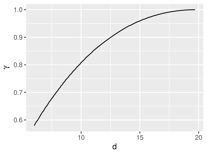
(a) The values of $\gamma=\sup_{x^{2}+y^{2}<d}\Gamma(x,y)$ when $d$ ranges over $(6,2\pi^{2})$, calculated numerically.

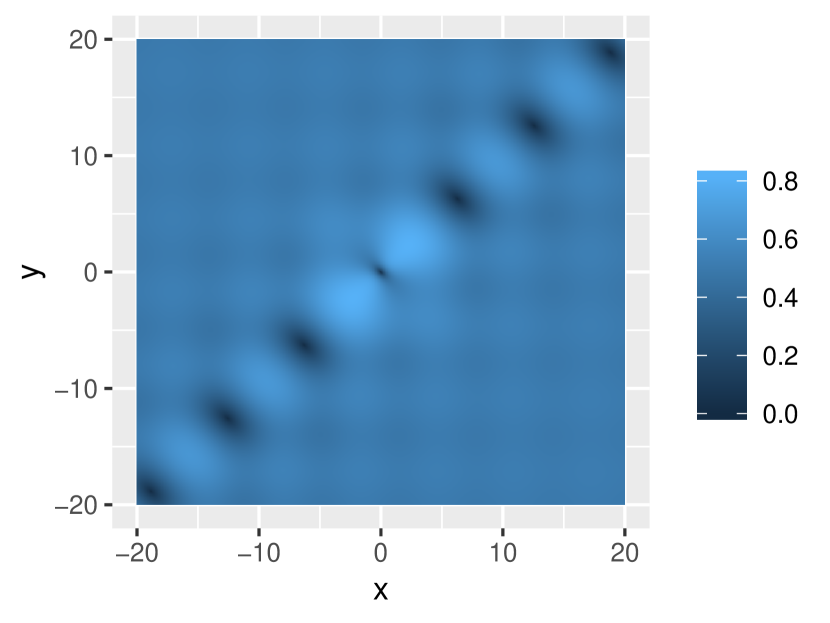
(b) A heat map of $\Gamma(x,y)^{r}\Lambda(x,y)^{1-r}$ for $r=0.395$. The supremum of this function is achieved at around $(-2.3,-2.3)$ and $(2.3,2.3)$, and is about $0.814$.

Figure 1: Features of $\Gamma$ and $\Lambda$, defined in (15) and (16).

We now provide an alternative bound by applying Theorem 2.6 (or Proposition 2.9) directly. By (14), $(B1)$ holds, and for every $(x,y)\in{\mathsf{X}}\times{\mathsf{X}}$,

$$\frac{PV(x)+PV(y)+1}{V(x)+V(y)+1}\leq\frac{x^{2}/2+y^{2}/2+4}{x^{2}+y^{2}+1}=:\Lambda(x,y)\,.$$ (16)

Let $\Gamma:{\mathsf{X}}\times{\mathsf{X}}\to[0,\infty)$ be defined as in (15). It’s easy to see that $(B2)$ is satisfied. To verify $(B3)$, we will evaluate $\sup_{(x,y)\in{\mathsf{X}}\times{\mathsf{X}}}\Gamma(x,y)^{r}\Lambda(x,y)^{1-r}$ for $r\in(0,1)$. Figure 1(b) plots the bivariate function $\Gamma(x,y)^{r}\Lambda(x,y)^{1-r}$ for a specific value of $r$. It is shown in Appendix B that, for each $r\in(0,1)$, one can find $\sup_{(x,y)\in{\mathsf{X}}\times{\mathsf{X}}}\Gamma(x,y)^{r}\Lambda(x,y)^{1-r}$ numerically through optimization over a compact subset of ${\mathsf{X}}\times{\mathsf{X}}$. When $r$ takes the value $0.395$ (which is optimal), an upper bound on the chain’s convergence rate is

$$\rho_{r}^{B}:=\sup_{(x,y)\in{\mathsf{X}}\times{\mathsf{X}}}\Gamma(x,y)^{r}\Lambda(x,y)^{1-r}\approx 0.814\,.$$

This is a significant improvement on $\rho_{r}^{A}$, which is constructed using standard drift and contraction conditions. The bound can be further improved to $\rho_{r}^{B}=0.577$ (with $r=0.382$) if we let

$$\Lambda(x,y)=\frac{PV(x)+PV(y)+1}{V(x)+V(y)+1}=\frac{[x/2-\sin(x)/2]^{2}+[y/2-\sin(y)/2]^{2}+3}{x^{2}+y^{2}+1}\,.$$ (17)

We note that it’s not really fair to compare the second $\rho_{r}^{B}$ with $\rho_{r}^{A}$, since the latter is based on the loosened drift inequality (14).

Of course, in more complicated problems, $\sup_{(x,y)\in{\mathsf{X}}\times{\mathsf{X}}}\Gamma(x,y)^{r}\Lambda(x,y)^{1-r}$ would likely be much more difficult to evaluate. Nevertheless, this example shows that generalized drift and contraction may contain useful information that is not available in their standard counterparts.

4.2 Gibbs chain for a random effects model

Let $q$ and $m$ be positive integers. Consider the random effects model

$$y_{ij}=\mu+\theta_{i}+e_{ij},\quad j=1,2,\dots,m,\text{ and }i=1,2,\dots,q,$$

where, independently, $\theta_{i}\sim\mbox{N}(0,\lambda_{\theta}^{-1})$, $e_{ij}\sim\mbox{N}(0,\lambda_{e}^{-1})$. Assume that $\mu$ has a flat prior, and that independently, $\lambda_{\theta}$ and $\lambda_{e}$ are a priori $\mbox{Gamma}(a_{1},b_{1})$ and $\mbox{Gamma}(a_{2},b_{2})$ distributed, respectively. Here, $a_{1},a_{2},b_{1},b_{2}$ are positive constants, and $b_{1}$ and $b_{2}$ are rate, rather than scale parameters. Denote the observed data $(y_{ij})_{ij}$ by $y$, and $(\theta_{1},\dots,\theta_{q})$ by $\theta$. The posterior density function of $(\mu,\theta,\lambda_{\theta},\lambda_{e})$ given $y$ is

$$\pi(\mu,\theta,\lambda_{\theta},\lambda_{e}|y)\propto \lambda_{e}^{mq/2}\exp\left[-\frac{\lambda_{e}}{2}\sum_{i=1}^{q}\sum_{j=1}^{m}(y_{ij}-\mu-\theta_{i})^{2}\right]$$

$$\times\lambda_{\theta}^{q/2}\exp\left(-\frac{\lambda_{\theta}}{2}\sum_{i=1}^{q}\theta_{i}^{2}\right)\lambda_{\theta}^{a_{1}-1}e^{-b_{1}\lambda_{\theta}}\lambda_{e}^{a_{2}-1}e^{-b_{2}\lambda_{e}},$$

where $\lambda_{\theta},\lambda_{e}>0$. It can be checked that this posterior is proper.

Fix $y\in\mathbb{R}^{qm}$. A Gibbs algorithm for sampling from $\pi(\cdot|y)$ can be constructed using the full conditionals $\pi_{1}(\mu,\theta|\lambda_{\theta},\lambda_{e},y)$ and $\pi_{2}(\lambda_{\theta},\lambda_{e}|\mu,\theta,y)$, whose exact form can be gleaned from $\pi(\cdot|y)$ (Román and Hobert, 2012). Let $(\mu^{(n)},\theta^{(n)},\lambda_{\theta}^{(n)},\lambda_{e}^{(n)}),\,n\in\mathbb{Z}_{+},$ be the corresponding Markov chain. Given $(\mu^{(n)},\theta^{(n)},\lambda_{\theta}^{(n)},\lambda_{e}^{(n)})=(\mu,\theta,\lambda_{\theta},\lambda_{e})$, the next state, $(\mu^{(n+1)},\theta^{(n+1)},\lambda_{\theta}^{(n+1)},\lambda_{e}^{(n+1)})$, depends only on $(\mu,\theta)$, and is drawn according to the following steps.

 

1. Draw $\lambda_{\theta}^{(n+1)}$ from $\mbox{Gamma}\left(q/2+a_{1},b_{1}+\sum_{i=1}^{p}\theta_{i}^{2}/2\right)$.

2. Draw $\lambda_{e}^{(n+1)}$ from

   $$\mbox{Gamma}\bigg{(}qm/2+a_{2},b_{2}+\sum_{i=1}^{q}\sum_{j=1}^{m}(y_{ij}-\mu-\theta_{i})^{2}/2\bigg{)}.$$

3. Draw $\mu^{(n+1)}$ from $\mbox{N}\left(\bar{y},(\lambda_{\theta}^{(n+1)}+m\lambda_{e}^{(n+1)})/(qm\lambda_{e}^{(n+1)}\lambda_{\theta}^{(n+1)})\right)$, where $\bar{y}=(qm)^{-1}\sum_{i,j}y_{ij}$.

4. Independently, draw $\theta_{i}^{(n+1)}$, $i=1,2,\dots,q$, from

   $$\mbox{N}\left(\frac{m\lambda_{e}^{(n+1)}(\bar{y}_{i}-\mu^{(n+1)})}{\lambda_{\theta}^{(n+1)}+m\lambda_{e}^{(n+1)}},\frac{1}{\lambda_{\theta}^{(n+1)}+m\lambda_{e}^{(n+1)}}\right),$$

   where $\bar{y}_{i}=m^{-1}\sum_{j=1}^{m}y_{ij}$.

 

As far as convergence properties are concerned, it suffices to consider the marginal chain $(\mu^{(n)},\theta^{(n)}),\,n\in\mathbb{Z}_{+}$. The state space of this chain is the $(q+1)$-dimensional Euclidean space, which we denote by ${\mathsf{X}}$. The transition kernel is

$$P\left((\mu,\theta),\mathrm{d}(\mu^{\prime},\theta^{\prime})\right)=\left[\int_{0}^{\infty}\int_{0}^{\infty}\pi_{1}(\mu^{\prime},\theta^{\prime}|\lambda_{\theta},\lambda_{e},y)\,\pi_{2}(\lambda_{\theta},\lambda_{e}|\mu,\theta,y)\,\mathrm{d}\lambda_{\theta}\,\mathrm{d}\lambda_{e}\right]\mathrm{d}\mu^{\prime}\mathrm{d}\theta^{\prime}\,,$$

and the stationary distribution $\varpi$ has density function

$$\frac{\mathrm{d}}{\mathrm{d}\mu\mathrm{d}\theta}\varpi(\mu,\theta)=\int_{0}^{\infty}\int_{0}^{\infty}\pi(\mu,\theta,\lambda_{\theta},\lambda_{e}|y)\,\mathrm{d}\lambda_{\theta}\,\mathrm{d}\lambda_{e}\,.$$

Let $\psi=\varrho$ be the metric given by

$$\varrho\left((\mu,\theta),(\mu^{\prime},\theta^{\prime})\right)=\sqrt{q(\mu-\mu^{\prime})^{2}+\sum_{i=1}^{q}(\theta_{i}-\theta_{i}^{\prime})^{2}}\,.$$

Qin and Hobert (2021+) applied Corollary 2.1 to study the convergence properties of the chain with respect to $W_{\psi}=W_{\varrho}$. Note that Qin and Hobert (2021+) parametrized $(\mu,\theta)$ differently, so their formula for $\varrho$ slightly differs from what is given here. In Appendix D of Qin and Hobert (2021+), the authors established (up to some minor differences) the following realizations of $(A1)$ and $(B2)$.

Lemma 4.1.

(Qin and Hobert, 2021+) For $(\mu,\theta)\in{\mathsf{X}}$, let

$$V(\mu,\theta)=\frac{1}{q}\sum_{i=1}^{q}(\theta_{i}+\bar{y}-\bar{y}_{i})^{2}+(\mu-\bar{y})^{2}\,.$$

Then

$$\varrho\left((\mu,\theta),(\mu^{\prime},\theta^{\prime})\right)\leq a\left[V(\mu,\theta)+V(\mu^{\prime},\theta^{\prime})+1\right],$$

$$PV(\mu,\theta)\leq\eta V(\mu,\theta)+L\,,$$

where $a=2q$,

$$\eta=\frac{2q+4}{qm+2a_{2}-2}+\frac{4}{q+2a_{1}-2}\,,$$

$$L=\frac{(q+2a_{1}+2)\sum_{i=1}^{q}(\bar{y}_{i}-\bar{y})^{2}+4b_{1}}{q(q+2a_{1}-2)}+\frac{q+2}{qm}\frac{\sum_{i=1}^{q}\sum_{j=1}^{m}(y_{ij}-\bar{y}_{i})^{2}+2b_{2}}{qm+2a_{2}-2}\,.$$

Moreover, for $((\mu,\theta),(\mu^{\prime},\theta^{\prime}))\in{\mathsf{X}}\times{\mathsf{X}}$,

$$W_{\varrho}(\delta_{(\mu,\theta)}P,\delta_{(\mu^{\prime},\theta^{\prime})}P)\leq\Gamma((\mu,\theta),(\mu^{\prime},\theta^{\prime}))\,\varrho\left((\mu,\theta),(\mu^{\prime},\theta^{\prime})\right)\,,$$

where

$$\Gamma((\mu,\theta),(\mu^{\prime},\theta^{\prime}))= \left\{\frac{4}{b_{1}}\left[\frac{b_{3}^{2}(q/2+a_{1})(q/2+a_{1}+1)}{b_{1}m^{2}(qm/2+a_{2}-1)(qm/2+a_{2}-2)}\wedge 1\right]\right.$$

$$+\left.\frac{8(q+2a_{1})}{b_{1}(qm+2a_{2}-2)}\right\}\sum_{i=1}^{q}(\bar{y}_{i}-\bar{y})^{2}$$

$$+\frac{5}{q/2+a_{1}-1}+\frac{4}{qm/2+a_{2}-1}$$

$$+\frac{2b_{3}q}{b_{1}m(qm+2a_{2}-2)}\wedge\frac{2q}{q+2a_{1}-2}+\frac{4q}{qm+2a_{2}-2}\,,$$

$$b_{3}:=b_{3}((\mu,\theta),(\mu^{\prime},\theta^{\prime}))=b_{2}+\frac{1}{2}\sum_{i=1}^{q}\sum_{j=1}^{m}(y_{ij}-\bar{y}_{i})^{2}+qmV(\mu,\theta)+qmV(\mu^{\prime},\theta^{\prime})\,.$$

For the remainder of this subsection, let $\eta$, $L$, $V$, and $\Gamma$ be defined as in Lemma 4.1. If $\eta<1$, then $(A1)$ holds. To make use of Corollary 2.1, one needs to define a coupling set, and find $\gamma$ and $K$ in $(A2)$. Let the coupling set be of the form

$$C=\left\{\left((\mu,\theta),(\mu^{\prime},\theta^{\prime})\right)\in{\mathsf{X}}\times{\mathsf{X}}:\,V(\mu,\theta)+V(\mu^{\prime},\theta^{\prime})<d\right\},$$

where $d>2L/(1-\eta)$. Let

$$\gamma=\sup_{((\mu,\theta),(\mu^{\prime},\theta^{\prime}))\in C}\Gamma\left((\mu,\theta),(\mu^{\prime},\theta^{\prime})\right),\quad K=\sup_{((\mu,\theta),(\mu^{\prime},\theta^{\prime}))\not\in C}\Gamma\left((\mu,\theta),(\mu^{\prime},\theta^{\prime})\right).$$

Then $(A2)$ holds with these parameters if $\gamma<1$ and $K<\infty$. Since $\Gamma((\mu,\theta),(\mu^{\prime},\theta^{\prime}))$ depends on its argument only through the value of $V(\mu,\theta)+V(\mu^{\prime},\theta^{\prime})$, we can let

$$\Gamma_{*}(v)=\Gamma\left((\mu,\theta),(\mu^{\prime},\theta^{\prime})\right)\text{ if }V(\mu,\theta)+V(\mu^{\prime},\theta^{\prime})=v\in[0,\infty)\,.$$

It is easy to obtain the formula of $\Gamma_{*}$ from that of $\Gamma$. From there, it is straightforward to establish that $\Gamma_{*}$ is a non-decreasing function, and that $\Gamma_{*}(v)$ remains constant when $v\geq v_{*}$ for some $v_{*}>0$ that is determined by $q,m,a_{1},a_{2},b_{1},b_{2},$ and $y$. Thus, $\gamma=\Gamma_{*}(d)$, and $K=\Gamma_{*}(v_{*})$.

In Qin and Hobert (2021+), it is shown that, if $m^{2}$ is a lot larger than $q^{3+\delta}$ for some $\delta>0$, then, under regularity conditions, one can choose an appropriate $d$ so that $(A1)$-$(A3)$ are all satisfied with $\eta,L,\gamma,K$ given above. The resultant bound via Corollary 2.1,

$$\rho_{r}^{A}=\left[\gamma^{r}(2L+1)^{1-r}\right]\vee\left[K^{r}\left(\frac{\eta d+2L+1}{d+1}\right)^{1-r}\right],$$

is shown to be asymptotically vanishing when $m^{2}/q^{3+\delta}\to\infty$. Although this bound is sharp asymptotically, it can be quite loose for fixed data sets. In what follows, we give a numerical illustration, and show how a bound based on Theorem 2.6 outperforms $\rho_{r}^{A}$.

Let $q=50$ and $m=1000$. Set the true value of $(\mu,\lambda_{\theta},\lambda_{e})$ to be $(1,10,5)$, and generate $y$ according to the random effects model. In our simulated data set,

$$\frac{1}{q}\sum_{i=1}^{q}(\bar{y}_{i}-\bar{y})^{2}=0.0712\,,\quad\frac{1}{qm}\sum_{i=1}^{q}\sum_{j=1}^{m}(y_{ij}-\bar{y}_{i})^{2}=0.199\,.$$

Set $a_{1}=a_{2}=b_{1}=b_{2}=1$. Using formulas in Lemma 4.1, one can find that $(A1)$ holds with $\eta=0.0821$ and $L=0.0787$. It can be shown that $\Gamma_{*}(v)$ is a non-decreasing function that stays constant when $v\geq v_{*}$, where $v_{*}$ is a number slightly smaller than 20. (See Figure 2.) This allows us to evaluate $(\gamma,K)$ for different choices of $d$ easily. Letting $d=1.35$ and $r=0.176$ yields the sharpest (smallest) bound $\rho_{r}^{A}=0.985$.

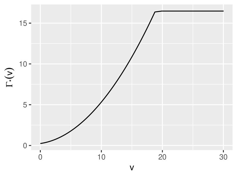
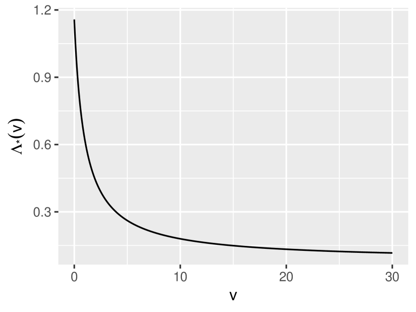
Figure 2: Graphs of $\Gamma_{*}$ and $\Lambda_{*}$.

We now couple Lemma 4.1 with Theorem 2.6 (or Proposition 2.9) instead to form a sharper convergence rate bound. We see from Lemma 4.1 that $(B1)$ and $(B2)$ hold with the functions $V$ and $\Gamma$. Let

$$\Lambda((\mu,\theta),(\mu^{\prime},\theta^{\prime}))=\frac{\eta[V(\mu,\theta)+V(\mu,\theta)]+2L+1}{V(\mu,\theta)+V(\mu,\theta)+1}.$$

As with $\Gamma((\mu,\theta),(\mu^{\prime},\theta^{\prime}))$, $\Lambda((\mu,\theta),(\mu^{\prime},\theta^{\prime}))$ depends on its argument only through the value of $V(\mu,\theta)+V(\mu^{\prime},\theta^{\prime})$. We can therefore let

$$\Lambda_{*}(v)=\Lambda\left((\mu,\theta),(\mu^{\prime},\theta^{\prime})\right)\text{ if }V(\mu,\theta)+V(\mu^{\prime},\theta^{\prime})=v\in[0,\infty)\,.$$

$\Lambda_{*}(v)=(\eta v+2L+1)/(v+1)$ is decreasing in $v$. (See Figure 2.) Moreover, recall that $\Gamma_{*}(v)$ is non-decreasing and constant when $v\geq 20$. For $r\in(0,1)$, let $\rho_{r}^{B}$ be the convergence rate bound constructed via Theorem 2.6, so that

$$\rho_{r}^{B} =\sup_{((\mu,\theta),(\mu^{\prime},\theta^{\prime}))}\Gamma\left((\mu,\theta),(\mu^{\prime},\theta^{\prime})\right)^{r}\Lambda\left((\mu,\theta),(\mu^{\prime},\theta^{\prime})\right)^{1-r}$$

$$=\sup_{v\in[0,20]}\Gamma_{*}(v)^{r}\Lambda_{*}(v)^{1-r}\,.$$

Let $r=0.335$. Then $\Gamma_{*}(v)^{r}\Lambda_{*}(v)^{1-r}$ is maximized when $v=18.78$, and this yields $\rho_{r}^{B}=0.687$, which is significantly smaller than $\rho_{r}^{A}=0.985$.

Acknowledgment. We thank the Editor, the Associate Editor, and two anonymous reviewers for helpful comments and suggestions. The second author was supported by NSF Grant DMS-15-11945.

Appendix

Appendix A Comparison of $\rho_{r}$ and Durmus and Moulines’s Geometric Rate Bound

We begin with a formal statement of Durmus and Moulines’s result.

Proposition A.1.

(Durmus and Moulines, 2015) Suppose that the metric $\varrho$ is bounded above by $1$, and that the following two conditions hold:

1. There exists a measurable function $\bar{V}:{\mathsf{X}}\to[1,\infty)$, $\eta^{\prime}\in[0,1)$, and $L^{\prime}\in\mathbb{R}$ such that

   $$P\bar{V}(x)\leq\eta^{\prime}\bar{V}(x)+L^{\prime}\,,\quad x\in{\mathsf{X}}\,.$$

2. There exists $\gamma^{\prime}\in[0,1)$ such that for each $(x,y)\in{\mathsf{X}}\times{\mathsf{X}}$,

   $$W_{\varrho}(\delta_{x}P,\delta_{y}P)\leq\begin{cases}\gamma^{\prime}\varrho(x,y)\,,&(x,y)\in C^{\prime}\,,\\ \varrho(x,y)\,,&(x,y)\not\in C^{\prime}\,,\end{cases}$$

   where the coupling set $C^{\prime}$ is defined to be $\big{\{}(x,y)\in{\mathsf{X}}\times{\mathsf{X}}:\,\bar{V}(x)+\bar{V}(y)\leq(2L^{\prime}+\delta^{\prime})/(1-\eta^{\prime})\big{\}}$, for some $\delta^{\prime}>0$  .

Then $P$ admits a unique stationary distribution $\varpi$. Moreover, for each $x\in{\mathsf{X}}$ and every $n\in\mathbb{Z}_{+}$,

$$W_{\varrho}(\delta_{x}P^{n},\varpi)\leq\left(\frac{1}{2}+\frac{1}{(\gamma^{\prime})^{2}}\right)\left(1+\frac{L^{\prime}}{1-\eta^{\prime}}\right)V(x)\left(\rho^{\mbox{\scriptsize{DM}}}\right)^{n}\,,$$

where

$$\rho^{\mbox{\scriptsize{DM}}}=\exp\left(-\frac{\log(1/\lambda)\log(1/\gamma^{\prime})}{\log J+\log(1/\gamma^{\prime})}\right)\,,$$

$\lambda=2L^{\prime}(1-\eta^{\prime})/(2L^{\prime}+\delta^{\prime})+\eta^{\prime}$, and $J=(2L^{\prime}+\delta^{\prime})/(1-\eta^{\prime})+2L^{\prime}/\lambda\,$.

The following result shows that Corollary 2.1 can always be used to improve upon $\rho^{\mbox{\scriptsize{DM}}}$.

Proposition A.2.

Assume that $\varrho$ is bounded, and $(C1)$ and $(C2)$ are satisfied. Then Corollary 2.1 can be used to construct an alternative convergence rate bound, $\rho_{r}$, such that $\rho_{r}<\rho^{\mbox{\scriptsize{DM}}}$.

Proof.

Since $\bar{V}\geq 1$, $(C1)$ implies that $L^{\prime}\geq(1-\eta^{\prime})\varpi\bar{V}\geq 1-\eta^{\prime}>0$ (see Hairer, 2018, Proposition 4.24). Thus, $\lambda\in(\eta^{\prime},1)$ and $J>1$.

We now translate $(C1)$ and $(C2)$ into $(A1)$-$(A3)$ and apply Corollary 2.1. Take $\psi=\varrho$ and $V=\bar{V}-1/2$. Then by $(C1)$ and the boundedness of $\psi$, $(A1)$ holds with $a=1$, $\eta=\eta^{\prime}$, and $L=L^{\prime}+\eta^{\prime}/2-1/2$. (Note that $L\geq 0$.) Take $d=(2L+\delta^{\prime})/(1-\eta)$, and set

$$C=\big{\{}(x,y)\in{\mathsf{X}}\times{\mathsf{X}}:\,V(x)+V(y)<d\big{\}}=\bigg{\{}(x,y)\in{\mathsf{X}}\times{\mathsf{X}}:\,\bar{V}(x)+\bar{V}(y)<\frac{2L^{\prime}+\delta^{\prime}}{1-\eta^{\prime}}\bigg{\}}\subset C^{\prime}\,.$$

By $(C2)$, condition $(A2)$ holds with $\gamma=\gamma^{\prime}$, $K=1$, and $C$ given above. Since $K=1$, $(A3)$ holds. Corollary 2.1, along with Remark 2.3, states that the chain’s $\varrho$-induced Wasserstein distance to its unique stationary distribution decreases at a geometric rate of (at most)

$$\rho_{r}=\big{[}\gamma^{r}(2L+1)^{1-r}\big{]}\vee\left(\frac{\eta d+2L+1}{d+1}\right)^{1-r}\,,$$

where

$$r\in\bigg{(}\frac{\log(2L+1)}{\log(2L+1)+\log(1/\gamma)},1\bigg{)}\;.$$

Note that

$$\frac{\eta d+2L+1}{d+1}=\eta^{\prime}+\frac{2L^{\prime}}{d+1}=\lambda\,.$$

Now set

$$r=\frac{\log(2L+1)+\log(1/\lambda)}{\log(2L+1)+\log(1/\lambda)+\log(1/\gamma)}\;.$$

A direct calculation shows that, with this value of $r$, we have

$$\gamma^{r}(2L+1)^{1-r}=\lambda^{1-r}=\exp\left(-\frac{\log(1/\lambda)\log(1/\gamma^{\prime})}{\log(2L+1)+\log(1/\lambda)+\log(1/\gamma^{\prime})}\right).$$

It follows that

$$\rho_{r}=\exp\left(-\frac{\log(1/\lambda)\log(1/\gamma^{\prime})}{\log(2L+1)+\log(1/\lambda)+\log(1/\gamma^{\prime})}\right).$$

Since $L^{\prime}\geq 1-\eta^{\prime}$, one has $J\lambda>2\lambda+2L^{\prime}>\eta^{\prime}+2L^{\prime}=2L+1$. As a result, $0<\log(2L+1)+\log(1/\lambda)<\log J$, which implies that $\rho_{r}<\rho^{\mbox{\scriptsize{DM}}}$. ∎

Finally, as argued at the end of Section 2, if $\rho_{r}$ is calculated based on a set of generalized drift and contraction conditions, then it may be further improved. As demonstrated in Section 4, the convergence rate bound in Theorem 2.6 can be considerably shaper than that in Corollary 2.1, and thus, substantially sharper than $\rho^{\mbox{\scriptsize{DM}}}$ as well.

Appendix B Finding $\rho_{r}^{B}$ for the Perturbed Linear Autoregressive Chain

Let ${\mathsf{X}}=\mathbb{R}$, and consider the linear autoregressive chain perturbed by a trigonometric term from Section 4. We now explain how to find

$$\rho_{r}^{B}=\sup_{(x,y)\in{\mathsf{X}}\times{\mathsf{X}}}\Gamma(x,y)^{r}\Lambda(x,y)^{1-r}\,,\quad r\in(0,1)\,,$$

where $\Lambda$ and $\Gamma$ are, respectively, given by (16) and (15). The main result is as follows.

Proposition B.1.

Let $\Lambda$ and $\Gamma$ be defined as in (16) and (15). Then for any $r\in(0,1)$,

$$\arg\max_{(x,y)\in{\mathsf{X}}\times{\mathsf{X}}}\Gamma(x,y)^{r}\Lambda(x,y)^{1-r}\subset C_{0}:=\{(x,y):\,x^{2}+y^{2}\leq 2\pi^{2}\}\,.$$

Proof.

Let $r\in(0,1)$ and $(x,y)\in({\mathsf{X}}\times{\mathsf{X}})\setminus C_{0}$ be arbitrary. It suffices to show that there exists $(x^{\prime},y^{\prime})\in C_{0}$ such that

$$\Gamma(x,y)^{r}\Lambda(x,y)^{1-r}<\Gamma(x^{\prime},y^{\prime})^{r}\Lambda(x^{\prime},y^{\prime})^{1-r}\,.$$ (18)

By the mean value theorem and periodicity, there exists a point $\xi\in[x,y]$ (or $[y,x]$), as well as a point $\xi^{\prime}\in[-\pi,\pi]$ such that

$$\Gamma(x,y)=\frac{1}{2}-\frac{\cos\xi}{2}=\frac{1}{2}-\frac{\cos\xi^{\prime}}{2}=\Gamma(\xi^{\prime},\xi^{\prime})\,.$$

Note that $(\xi^{\prime},\xi^{\prime})\in C_{0}$. Moreover, it’s easy to verify that $\Lambda(x,y)<\Lambda(\xi^{\prime},\xi^{\prime})$. As a result, (18) holds with $x^{\prime}=y^{\prime}=\xi^{\prime}$. ∎

Proposition B.1 implies that, to maximize $\Gamma(x,y)^{r}\Lambda(x,y)^{1-r}$ over ${\mathsf{X}}\times{\mathsf{X}}$, we only need to restrict our attention to the compact set $C_{0}$. Since the objective function is uniformly continuous on $C_{0}$, we can solve the problem by optimizing over a sufficiently fine grid.

Finally, assume instead that $\Lambda$ is given by (17). The analog of Proposition B.1 is as follows.

Proposition B.2.

Let $\Lambda$ and $\Gamma$ be defined as in (17) and (15). Then for any $r\in(0,1)$,

$$\arg\max_{(x,y)\in{\mathsf{X}}\times{\mathsf{X}}}\Gamma(x,y)^{r}\Lambda(x,y)^{1-r}\subset C^{\prime}_{0}:=\{(x,y):\,|x|\leq 26,\,|y|\leq 26\}\,.$$

Proof.

Let $r\in(0,1)$ and $(x,y)\in({\mathsf{X}}\times{\mathsf{X}})\setminus C^{\prime}_{0}$ be arbitrary. It suffices to show that there exists $(x^{\prime},y^{\prime})\in C^{\prime}_{0}$ such that (18) holds. As in the proof of Proposition B.1, there exists a point $\xi\in[-2\pi,-\pi]\cup[\pi,2\pi]$ such that $\Gamma(x,y)=\Gamma(\xi,\xi)$. Note that $(\xi,\xi)\in C^{\prime}_{0}$. Moreover, $\xi$ and $\sin\xi$ have opposite signs. Thus,

$$\Lambda(\xi,\xi)\geq\frac{\xi^{2}/2+3}{2\xi^{2}+1}>0.284\,.$$

Since $(x,y)\not\in C^{\prime}_{0}$, we have $|x|>26$ or $|y|>26$. Without loss of generality, assume that the former holds. Then $|x|<x^{2}/26$, and $|y|+(x^{2}+1)/|y|>52$. It follows that

$$\Lambda(x,y) \leq\frac{(|x|+1)^{2}/4+(|y|+1)^{2}/4+3}{x^{2}+y^{2}+1}$$

$$=0.25+\frac{0.5|x|+0.5|y|+3.25}{x^{2}+y^{2}+1}$$

$$<0.25+\frac{x^{2}}{52(x^{2}+y^{2}+1)}+\frac{0.5}{|y|+(x^{2}+1)/|y|}+\frac{3.25}{x^{2}+y^{2}+1}$$

$$<0.25+1/52+0.5/52+3.25/(26^{2}+1)$$

$$<0.284\,.$$

Hence, $\Lambda(x,y)<\Lambda(\xi,\xi)$, and (18) holds with $(x^{\prime},y^{\prime})=(\xi,\xi)$. ∎

References

- Billingsley (1999) Billingsley, P. (1999). Convergence of Probability Measures. 2nd ed. John Wiley & Sons.
- Butkovsky (2014) Butkovsky, O. (2014). Subgeometric rates of convergence of Markov processes in the Wasserstein metric. Annals of Applied Probability 24 526–552.
- Douc et al. (2004) Douc, R., Fort, G., Moulines, E. and Soulier, P. (2004). Practical drift conditions for subgeometric rates of convergence. Annals of Applied Probability 14 1353–1377.
- Douc et al. (2018) Douc, R., Moulines, E., Priouret, P. and Soulier, P. (2018). Markov Chains. Springer.