Disentangling Flavor Violation in the Top–Higgs Sector at the LHC
Abstract
We study the LHC phenomenology of flavor changing Yukawa couplings between the top quark, the Higgs boson, and either an up or charm quark. Such or couplings arise for instance in models in which the Higgs sector is extended by the existence of additional Higgs bosons or by higher dimensional operators. We emphasize the importance of anomalous single top plus Higgs production in these scenarios, in addition to the more widely studied decays. By recasting existing CMS searches in multilepton and diphoton plus lepton final states, we show that bounds on are improved by a factor of 1.5 when single top plus Higgs production is accounted for. We also recast the CMS search for vector boson plus Higgs production into new, competitive constraints on and couplings, setting the limits of and .
We then investigate the sensitivity of future searches in the multilepton channel and in the fully hadronic channel. In multilepton searches, studying the lepton rapidity distributions and charge assignments can be used to discriminate between couplings, for which anomalous single top production is relevant, and couplings, for which it is suppressed by the parton distribution function of the charm quark. An analysis of fully hadronic production and decay can be competitive with the multilepton search at 100 fb-1 of 13 TeV data if jet substructure techniques are employed to reconstruct boosted top quarks and Higgs bosons. To show this we develop a modified version of the HEPTopTagger algorithm, optimized for tagging decays. Our sensitivity estimates on () at 100 fb-1 of 13 TeV data for multilepton searches, vector boson plus Higgs search and fully hadronic search are (), () and (), respectively.
Keywords:
Higgs Physics, Top Physics, Beyond Standard Model1 Introduction
Determining the properties of the newly-discovered Higgs boson is one of the major goals of the LHC physics program. Higgs interactions with fermions are of special interest since deviations from Standard Model (SM) predictions could point to the existence of new flavor dynamics not too far above the electroweak scale. Among the flavor violating Higgs couplings to quarks, the most promising place to look for new physics at high energy colliders are processes involving top quarks. On the one hand, all relevant indirect low energy constraints on such processes are necessarily based on loop suppressed observables [1]. On the other hand, the large number of top quarks produced at the LHC allows us to study even strongly suppressed contributions to top quark production and decay. Using this feature, the CMS collaboration has provided the best official upper limit on flavor violating couplings: from a combination of multilepton searches and diphoton plus lepton searches, the constraint is obtained at confidence level (CL) [2].
In the present work, we explore the LHC sensitivity to non-standard flavor violating top–Higgs interactions ( and ) further. Building upon related theoretical [3, 4, 5, 6, 7, 8] and experimental [9, 10, 11] studies, we explore three main directions: (1) We demonstrate the importance of the single top+Higgs production processes in addition to decays. (2) We demonstrate how these processes can be exploited to distinguish and couplings in leptonic events by studying lepton rapidity distributions and charge assignments. (3) we consider several novel search signatures including hadronic top decays and Higgs decays to and . While this leads to more challenging signatures requiring efficient discrimination against the large SM backgrounds, the final sensitivity is compensated by increased signal yields.
The remainder of the paper is organized as follows: In Sec. 2 we set up the notation and introduce our main physics ideas. Then we explore and quantify these insights in more detail using several top and Higgs decay modes. Multilepton searches [4] are particularly sensitive to final states, and in Sec. 3.1 we recast a recent CMS analysis [9] to constrain these final states. In doing so, we demonstrate the importance of including the anomalous single top production process . In Sec. 3.2 we recast a recent CMS search [2] for flavor violating coupling in the diphoton plus lepton final state to set an improved bound on coupling. In Sec. 3.3 we show that a competitive sensitivity can be obtained focusing specifically on decays by recasting a CMS search [12] for associate and production. We then proceed to future searches, showing in Sec. 4.1 how a detailed analysis of kinematic distributions in multilepton searches can be used to improve the sensitivity to both and couplings, and to discriminate between them. Finally, in Sec. 4.2, we develop a search strategy for the fully hadronic final state , where for highly boosted processes jet substructure techniques can be employed to identify top quarks and Higgs bosons. We summarize our results in Sec. 5.
2 Flavor Violating Top–Higgs Couplings
We parameterize the flavor violating top–Higgs interactions in the up-quark mass eigenbasis as
| (1) |
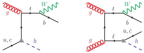
At tree level, this Lagrangian gives rise to the non-standard 3-body Higgs boson decays as well as the more interesting 2-body top quark decays , where (see Fig. 1). Neglecting the light quark masses and assuming the top quark decay width is dominated by the SM value of , the approximate relation between the relevant branching ratios and the flavor violating Yukawa couplings is given by
| (2) |
with the top quark mass , the mass , the Higgs mass , and the Fermi constant . The above expression is based on the leading order formulae for both the and decay rates. The NLO QCD correction to the branching ratio (in the pole top mass scheme) are included through the factor , calculated using the known corrections to the [13, 14] and decay widths [15]. We note that values of correspond to . Top quark pair production followed by an anomalous decay has a total cross section of
| (3) |
at the TeV energy LHC, where we have used the QCD NNLO values of pb [16].
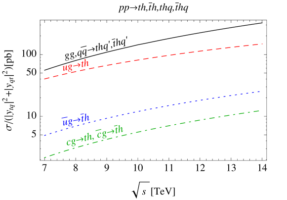
The interactions in Eq. 1 also contribute to associated single top plus Higgs production at the LHC. In particular the effects of and are significant due to the large flux of valence -quarks. The production cross-section is comparable in magnitude to (3):
| (4) |
where we have used the NLO QCD result of [5, 18]. The cross section for the conjugate process antitop + Higgs production is roughly an order of magnitude smaller, and processes induced by couplings are even more suppressed as illustrated in Fig. 2. This implies that, for a given center of mass energy and luminosity, the sensitivity to couplings is in general better than the one to couplings.
In addition, the presence or absence of a significant contribution of production in single top plus Higgs final states can be used to distinguish between couplings to up quarks and couplings to charm quarks. A good discriminating variable is the Higgs boson pseudorapidity, , as illustrated in Fig. 3.
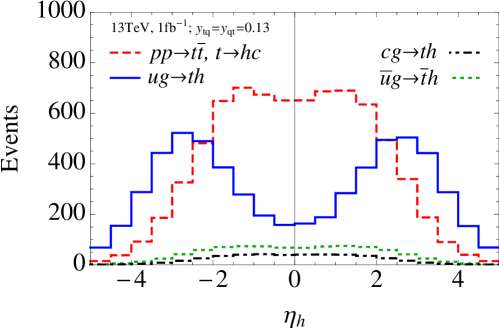
The relevance of this variable can be understood from the fact that in scattering, the interaction products tend to be boosted in the direction of the incoming valence quark, which on average carries a larger fraction of the proton momentum than the gluon. In addition, the Higgs boson in such a scattering process is preferentially produced in the direction of the up quark in the partonic center of mass frame due to angular momentum conservation combined with the quark chirality flip at the vertex. These effects add up to make the resulting distribution peak at large rapidities. For initial states not containing valence quarks (gluon fusion-induced production as well as single top + Higgs production in , , or collision), both the top quark and Higgs boson are produced more centrally. Another useful handle on tagging single top plus Higgs production in searches with leptonic top decays is the enhanced abundance of positively charged leptons.
In the following sections we demonstrate the relevance of associated production for probing flavor violating top–Higgs couplings using several promising experimental signatures. Unless stated otherwise explicitly, all our numerical results are obtained using a FeynRules v1.6.16 [19] implementation of the effective interactions in Eq. (1) and using MadGraph 5, v1.5.11 (and v2.0.0-beta3) [20] for MC simulation. Furthermore we employ Pythia v6.426 [21] for parton showering and hadronization, while Delphes v3.0.9 (and v3.0.5) [22] is used for detector simulation.
3 Improved Limits on and Couplings from Current LHC Searches
3.1 Recasting the CMS Multilepton Search
Multilepton searches at the LHC profit from relatively low SM backgrounds and are therefore sensitive to new physics processes producing final states with many leptons. A good example is a final state with a top quark and a Higgs boson [4], where the top quark decays to , and the 126 GeV Higgs boson decays to final states with up to four leptons. The relevant processes are , , , , and with branching ratios , , , and , respectively [23]. Single top + Higgs production can thus yield up to five leptons, so that multilepton searches can be expected to constrain anomalous flavor violating top–Higgs interactions.
In this section, we recast a recent CMS search for anomalous production of final states with three or more isolated leptons [9], based on of data at TeV. Data are binned into exclusive categories according to the lepton flavor, the missing transverse energy , the scalar sum of the transverse momenta of all the jets , the existence of -tagged jets, and the presence or absence of opposite sign, same flavor (OSSF) light lepton pairs. Events with an OSSF pair are further divided into “below Z”, “on Z” and “above Z” categories based on the invariant mass of the OSSF lepton pair relative to the mass.
CMS has already interpreted this search as a constraint on the anomalous coupling [9], considering top pair production followed by anomalous top decay to . However, the CMS search does not include contributions from single top + Higgs production, which is irrelevant for couplings, but very important for couplings. Therefore, we study in the following the importance of associated production for constraining anomalous couplings.
We simulate the processes followed by or decay, as well as and using MadGraph. We rescale the leading order cross sections to the corresponding higher order QCD results. In particular, events are generated using the default MadGraph dynamical factorization and renormalization scales, and the final cross section is rescaled to pb [16]. Single top plus Higgs events are generated using factorization and renormalization scales fixed to , and a QCD correction factor of is applied [5]. Higgs bosons and gauge bosons are decayed using BRIDGE v2.24 [24], where the SM Higgs branching ratios are taken from [23]. Showering and hadronization are simulated in Pythia, and Delphes is used for detector simulation. We have modified the default implementation of the CMS detector in Delphes by switching to the anti- jet algorithm with distance parameter , by changing the light charged lepton isolation criteria in accordance with [9], and by implementing the tagging efficiencies and mistag rates given in [9] for the medium working point of the Combined Secondary Vertex (CSV) algorithm.
We apply analysis cuts in accordance with those used in the CMS multilepton search [9]. In particular, we require the leading charged lepton in each event to have GeV. Additional light charged leptons must have GeV, and all of them must be within . Events are rejected if they have an OSSF lepton pair with invariant mass GeV. Jets are required to have and GeV, and an angular distance from any isolated charged lepton candidates.
| OSSF pair | ||||||||
|---|---|---|---|---|---|---|---|---|
| 1. | below Z | 10.8 | 6.7 | 48 | ||||
| 2. | no OSSF | 4.4 | 3.0 | 29 | ||||
| 3. | below Z | 6.8 | 3.8 | 34 | ||||
| 4. | no OSSF | 4.2 | 2.5 | 29 | ||||
| 5. | below Z | 2.5 | 0.6 | 10 | ||||
| 6. | below Z | 2.0 | 0.4 | 5 | ||||
| 7. | below Z | 0 | 9.2 | 5.1 | 142 | |||
| 8. | no OSSF | 0 | 4.0 | 2.5 | 35 | |||
| 9. | above Z | 1.9 | 1.2 | 17 |
The results of our simulations are presented in Table 1. The most sensitive bins have exactly three isolated leptons and no hadronically decaying taus. Signal predictions are given for which corresponds to . Taking into account the fact that we use a simplified detector simulation, the predictions for top pair production , are in good agreement with the results obtained by CMS [9]. This serves as an important cross check of our simulation.
Table 1 confirms that for couplings the contribution of associated production to the signal, , is of the same order as the contribution from production followed by decay, , as advocated before. Using the CLs method [25], we derive the new 95% CL limits
| (5) | ||||
| (6) |
The corresponding limits on the flavor violating couplings are and . We have checked that the minor difference between Eq. (5) and the CMS result is due to the contributions of hadronic tau decays which we do not include in our analysis. Our main conclusion, namely that the limit on is more stringent than the limit on by a factor of 1.5 due to associated production, is unaffected by this omission.
3.2 Recasting the CMS Diphoton plus Lepton Search
Recently, CMS has interpreted a search for extended Higgs sectors in the diphoton plus lepton final state [26] as a constraint on flavor violating coupling [2], using of data collected at TeV. In the following, we use this search to constrain also couplings, taking into account the contribution from associated top plus Higgs production.
| 1. | 3.2 | 1.3 | 1 | |||
| 2. | 2.2 | 0.92 | 2 | |||
| 3. | 1.9 | 0.83 | 2 | |||
| 4. | 0 | 2.4 | 1.1 | 7 | ||
| 5. | 0.82 | 0.49 | 0 | |||
| 6. | 0 | 0.87 | 0.52 | 1 | ||
| 7. | 0 | 1.6 | 0.64 | 29 |
We use MadGraph to simulate the signal processes induced by couplings, namely, top pair production followed by anomalous or decay as well as associated single (and ) plus Higgs production. Leptonic top decays as well as Higgs decays to pairs of photons are simulated using MadGraph where the implementation of the effective interaction is adopted from [27]. The SM branching ratio for is taken to be [23]. We rescale the leading order cross sections to the corresponding higher order QCD corrected results as in Sec. 3.1. We simulate showering and hadronization effects in Pythia and detector effects in Delphes. We use the same implementation of the CMS detector in Delphes as in Sec. 3.1.
We closely follow the CMS search [2] in our analysis. In particular, we require one light charged lepton with GeV and . We require two photons with GeV ( GeV) for the leading (next to leading) photon and . The diphoton invariant mass is required to be between and GeV. Events are categorized into exclusive categories based on and on the presence or absence of a bottom-tagged jet.
We summarize the results of our simulations in Table 2. The most sensitive bins have a -tagged jet and no hadronically decaying taus [2]. The predictions for signal yields are given for which corresponds to . We validate our simulation by closely reproducing the predictions for top pair production followed by anomalous top decay, , presented in Table 3 of [2]. Finally, the contribution from associated production, , is competitive and thus important in the case of flavor violating interactions. As before, we employ the CLs method [25] to derive the new 95% CL limits
| (7) |
where the corresponding limits on the flavor violating Yukawa couplings are and . The obtained limit on couplings is in a good agreement with the CMS result [2].
The search in the diphoton plus lepton final state sets the most competitive current bounds on flavor violating interactions and will remain very promising for future studies. The current search is mainly limited by statistics, so that further improvements are expected at larger integrated luminosities. Improvements are also expected in the data-driven background estimation by fitting the background shapes from the sidebands around the Higgs mass window in the diphoton invariant mass [26]. We estimate the expected sensitivity to at 100 fb-1 (3000 fb-1) and TeV to improve by a factor (), based on naive scaling in cross section and luminosity. Our rough estimate is in a good agreement with the dedicated study performed by the ATLAS collaboration [28].
Furthermore, the advantage of this search with respect to other searches is an explicit reconstruction of the Higgs boson which would be very useful in the case of a positive signal. Finally, as we will show in Sec. 4.1, the origin of the signal ( or couplings) could be disentangled by studying the Higgs pseudorapidity distribution and the charges of the light charged lepton from the top decay.
3.3 Recasting the CMS Search for Vector Boson + Higgs Production
In [12], the CMS collaboration has searched for Higgs bosons produced in association with a or and decaying to . This final state is very similar to the one obtained from single top + Higgs production, followed by and , and from production with one of the top quarks decaying to . The CMS search can thus be recast to set limits on the flavor changing and couplings that we are interested in here.
In doing so, we consider only the final state consisting of two light leptons (electrons or muons) and one hadronically decaying . This final state turns out to be more sensitive than (one light lepton and two hadronic ’s) in the CMS search, and is therefore also expected to give the best sensitivity in our case. In particular, the main competing factors affecting the relative importance of the and channels—the small leptonic branching ratio of the and the larger fake rate for hadronic ’s—affect the channel in the same way as our final state. CMS also consider final states with four light charged leptons, with at least two of them consistent with a decay. Since in the case of production or production followed by decay, only events with the suppressed Higgs decay could contribute to this final state, we do not consider it here.
We simulate the signal and the top and Higgs decays in MadGraph. Since in [12], CMS have used 5.0 fb-1 of data collected at TeV as well as 19.5 fb-1 of data collected at TeV, we simulate events for both center-of-mass energies. We rescale the leading order cross sections to the corresponding higher order QCD corrected results as in Sec. 3.1. We use TAUOLA v2.5[29] to decay the leptons and Pythia for parton showering and hadronization. We choose Delphes as a detector simulation, and we adapt the default implementation of the CMS detector by adjusting the -dependent tagging efficiency and mistag rate to the values given in [30] for the loose working point of the HPS (“hadron plus strips”) algorithm.
In accordance with [12] we use the following cuts; we require exactly two light leptons (electrons or muons), with the of the leading lepton larger than 20 GeV and that of the subleading lepton larger than 10 GeV. Muons are required to have a pseudorapidity , while for electrons the requirement is . The leptons must have the same charge to suppress backgrounds, and the flavor combinations and are allowed while events are vetoed. We also require one -tagged jet with GeV and . Extra jets are allowed, but events containing a -tagged jet with GeV and are vetoed to suppress backgrounds. Finally, the scalar sum of the lepton and ’s is required to be larger than 80 GeV.
 |
 |
| Current limit | ||||
|---|---|---|---|---|
| Future sensitivity |
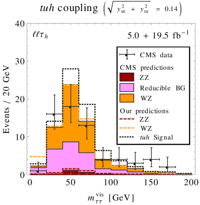
To verify our simulation and our analysis, we have also simulated the Standard Model and backgrounds. Fig. 4 shows that our background predictions are in excellent agreement with the CMS data [12] and with background predictions by CMS. The figure also shows that a signal induced by flavor violating top–Higgs couplings at the current upper limit from CMS would lead to a sizeable excess of events. Quantifying this excess using the CLs method [25], we find the new 95% CL limits on flavor-violating top Yukawa couplings given in Table 3.
In the same table, we also give an estimate for the sensitivity of a future search using 100 fb-1 of 13 TeV LHC data and assuming identical cuts as in the analysis at 7 and 8 TeV. Since we cannot reliably model the reducible background from fake leptons, we assume it to be of the same size and have the same distribution as the background. The larger instantaneous luminosity and larger pileup at 13 TeV may require somewhat harder cuts and could lead to increased backgrounds from misidentified jets. We expect, however, that these complications can be offset by further improvements of the analysis, for instance using multivariate techniques.
4 Sensitivity of Future Searches
4.1 Future Multilepton Searches and Discrimination between and Couplings
In this section, we study the potential of future multilepton searches at 13 TeV center of mass energy to constrain anomalous interactions or to establish their existence. Furthermore, we study the ability to differentiate between and couplings based on the presence or absence of large contributions from associated single top plus Higgs production to the signal.
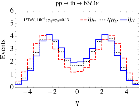
We closely follow the analysis conducted in Sec. 3.1. In particular, we use the same lepton and jet reconstruction and isolation requirements as before. An optimized search at 13 TeV will have slightly different requirements, such as somewhat higher lepton thresholds, but we expect these to have only a minor impact on the sensitivity. We require exactly three light charged leptons in the final state. In order to differentiate between and signals, we bin the data further with respect to two variables: (1) the total sum of lepton charges ,111For related work see [31]. and (2) the pseudorapidity of the opposite charge dilepton system with the smallest angular distance . We expect a signal to have a preference for due to a substantial contribution from the process , while couplings yield approximately equal numbers of events with and . The idea behind the variable is that the two leptons with the smallest have the highest probability of originating from decay (as opposed to a semileptonic top decay), so that is an approximation to the pseudorapidity of the Higgs boson in the event, which we have seen in Sec. 2 to be a promising discriminant between and couplings. To illustrate the correlation between and the Higgs rapidity , we have carried out a parton level simulation of the process followed by and using MadGraph. In Fig. 5 we show the resulting distributions for , and . The latter quantity is defined as the rapidity of the dilepton system that actually originates from Higgs decay. We see that, indeed, nicely follows . Since we have already seen in Sec. 2 and Fig. 3 that is an efficient discriminator between and couplings, we can expect the same to hold for the experimentally accessible quantity . We use two bins in : and .
| on OSSF | 61 | 67 | 20 | 19 | 2.5 | 7.4 | |||
| 58 | 59 | 16 | 18 | 2.7 | 13 | ||||
| 82 | 83 | 22 | 22 | 3.6 | 9.6 | ||||
| 77 | 88 | 20 | 21 | 2.9 | 16 | ||||
| 34 | 32 | 7.0 | 5.7 | 1.2 | 3.7 | ||||
| 35 | 27 | 4.3 | 4.5 | 0.9 | 6.6 | ||||
| 17 | 25 | 3.6 | 3.6 | 0.1 | 0.8 | ||||
| 19 | 21 | 2.3 | 2.1 | 0.2 | 1.3 | ||||
| 35 | 30 | 4.7 | 5.3 | 0.2 | 0.8 | ||||
| 29 | 27 | 4.0 | 3.7 | 0.2 | 1.7 | ||||
| 26 | 18 | 2.8 | 2.9 | 0.6 | 1.5 | ||||
| 21 | 18 | 1.8 | 1.8 | 0.2 | 2.8 | ||||
| below Z | 100 | 96 | 51 | 49 | 7.6 | 22 | |||
| 83 | 93 | 42 | 42 | 7.3 | 34 | ||||
| 36 | 42 | 12 | 15 | 1.8 | 8.6 | ||||
| 40 | 41 | 11 | 9.9 | 2.2 | 13 | ||||
| 36 | 31 | 9.5 | 11 | 0.8 | 2.3 | ||||
| 23 | 20 | 7.8 | 10 | 0.6 | 3.7 | ||||
| 22 | 20 | 8.1 | 7.7 | 0.6 | 3.1 | ||||
| 15 | 14 | 4.3 | 4.6 | 0.5 | 6.1 | ||||
| above Z | 42 | 39 | 7.8 | 7.9 | 1.3 | 3.1 | |||
| 62 | 55 | 7.1 | 7.4 | 1.4 | 6.4 | ||||
| 41 | 50 | 9.9 | 6.9 | 1.0 | 4.2 | ||||
| 68 | 71 | 8.2 | 8.8 | 1.2 | 7.9 | ||||
| 20 | 21 | 2.1 | 2.3 | 0.5 | 2.6 | ||||
| 26 | 34 | 2.2 | 3.0 | 0.3 | 4.2 | ||||
| 21 | 17 | 1.7 | 1.2 | 0.1 | 0.3 | ||||
| 29 | 27 | 1.7 | 1.9 | 0.0 | 0.9 | ||||
| 22 | 28 | 2.4 | 2.6 | 0.2 | 0.3 | ||||
| 30 | 25 | 1.5 | 2.0 | 0.2 | 1.1 | ||||
| 15 | 18 | 1.4 | 1.3 | 0.2 | 1.0 | ||||
| 22 | 20 | 1.7 | 0.7 | 0.1 | 2.1 | ||||
Recalling the results of the analysis from Sec. 3.1 based on real CMS data, we concentrate on the event categories that we have found to be most sensitive: we consider only events with exactly three light charged leptons that fall into the “above Z” , “no OSSF” or “below Z” categories; in the latter case we also require GeV. Moreover, we require at least one -tagged jet. The dominant background in all categories is from fully leptonic events with a jet misidentified as a lepton [9]. We simulate at 8 TeV and 13 TeV center of mass energy using MadGraph and normalize the corresponding cross sections to the NNLO QCD corrected values of pb [16], respectively. Showering, hadronization and detector effects are simulated using Pythia and Delphes. Following the procedure recommended by CMS [9], we model fake leptons by randomly converting an isolated track to a lepton with the measured conversion probability of 0.007 (0.006) for electron (muon) tracks. To check the validity of this approach, we first compare our 8 TeV predictions to CMS results [9] in the dilepton control region that requires an opposite-sign pair. We obtain good agreement with the and distributions shown in Fig. 1 and Fig. 2 of [9]. Second, we have checked that we agree with CMS, at the level of 30–40%, on the distributions (provided in [9]) of the background in the “noOSSF”, “above Z” and “below Z” signal regions with low and high and with at least one -tagged jet. The main difficulty in reproducing the background more precisely is the modeling of lepton misidentification. Therefore, our quantitative results should be considered with care, and a dedicated experimental analysis is clearly necessary to obtain more precise predictions. We note in passing that the irreducible SM background coming from associate top + Higgs production with a cross-section of fb at 13 TeV LHC222This value corresponds to the inclusive production cross section calculated in MadGraph using 5-flavor parton distribution functions and after applying a QCD correction factor of [32]. is only expected to become relevant once the sensitivity reaches .
Our predicted signal and background yields at 13 TeV center of mass energy are shown in Table 4 for an integrated luminosity of 100 fb-1, and for . The most sensitive bins fall into the “below Z” categories. It is worth noting that single top + Higgs production ( column in Table 4) tends to populate preferably bins with and , while the background ( column) and the signal ( column) are much more evenly distributed. This is of crucial importance in discriminating between the and signal hypotheses.
To estimate the achievable sensitivity and discovery reach for flavor violating top–Higgs couplings, we use the CLs method [25], treating all bins as statistically independent Poisson variables. We treat the overall normalization of the background as a nuisance parameter (positively correlated among all bins) to account for the uncertainty in our modeling of the lepton misidentification probability. We do not impose any a priori constraints on the nuisance parameter, i.e. we determine it in the analysis together with the signal parameters, taking advantage of the fine-grained binning of the simulated data. Since in a realistic experimental analysis, the misidentification rate can be measured from a control sample [9], our projected limits should be considered as very conservative.
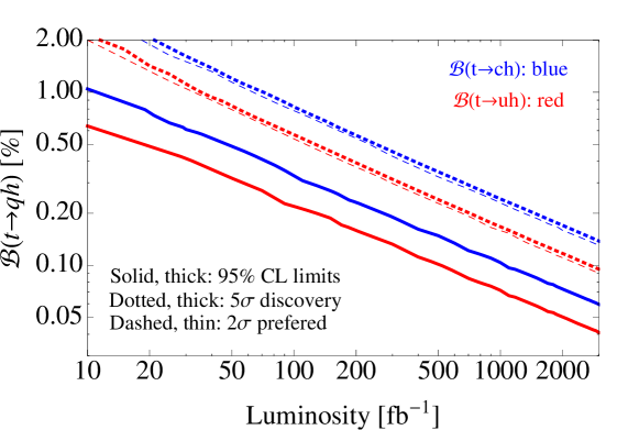
The results of our statistical analysis are plotted in Fig. 6. Expected CL limits on [] in the absence of a signal are shown as red (blue) thick solid curves. The expected discovery potential for a () signal is shown as a red (blue) thick dotted curve. The discrimination power between and couplings is shown as thin dashed curves. For pure () couplings above the red (blue) thin dashed curve, the opposite hypothesis of pure () couplings can be ruled out at the 95% CL.
From the coincidence of the thick dotted curves and the thin dashed ones we conclude that, if a signal is discovered (i.e. the BG only hypothesis is rejected at ), the discrimination power between and couplings is already at the level of . It is interesting that this remarkable performance is achieved in spite of the rather generic, unoptimized cuts in this multi-purpose multilepton analysis and of our rather conservative treatment of systematic uncertainties.
4.2 Searches in the Fully Hadronic Final State
The final state with the largest branching ratio in production and decay is the fully hadronic one. Modern jet substructure techniques [33, 34, 35] offer promising tools to extract this signal from the otherwise overwhelming background of QCD multijet events, SM and single top production and vector boson plus jets production. They are efficient when the top quarks and Higgs bosons constituting the signal are highly boosted so that the angular separation of their decay products is too small to be resolved by conventional jet algorithms. Instead, jet substructure methods use “fat jets”, i.e. jets with a very large radius . After the initial clustering, the fat jet is partially unclustered again to examine the invariant mass of its largest subclusters. Comparing these invariant masses to the masses of possible parent particles such as top quarks, Higgs bosons or bosons, the algorithm decides how probable it is that the fat jet was produced by one of these parent particles.
Here, we study the sensitivity of two analyses using jet substructure: (1) a search for events with one SM top decay and one flavor violating decay ; (2) a search for anomalous single top + Higgs production with SM top decay and .
In both analyses, we use the Cambridge-Aachen algorithm [36] as implemented in FastJet 3.0.3 [37] to cluster fat jets with a radius and a minimum transverse momentum GeV. We run HEPTopTagger v1.0 [34, 35] with default settings on these jets to identify those which are most likely to originate from a SM hadronic top decay . HEPTopTagger imposes cuts on the invariant masses of the three main subjets of the top candidate, requiring that two of them reconstruct to a , while all three together yield the top mass. Moreover, their combined has to exceed 200 GeV. In addition to these kinematic cuts, we also require the subjet that is most likely to originate from the quark to contain a tag (see Appendix A for details on our implementation of -tagging).
4.2.1 Analysis 1: tag + top tag
To identify flavor violating decays for analysis 1) and assign a “” tag to the corresponding fat jets, we reprocess all fat jets using a modified version of HEPTopTagger, which we have optimized for this non-standard decay mode (see Appendix A). We require a tag in each of the two subjets most likely to originate from the Higgs decay. We consider two different working points for our tagger: a loose one with very robust kinematic cuts on the subjet invariant masses, and a tight one with somewhat more restrictive cuts that make it more efficient at suppressing backgrounds, but also more prone to systematic uncertainties in our simulations. Details on the kinematic cuts are given in Appendix A. A tight tag moreover requires that the fat jet does not simultaneously carry a regular top tag.
Event selection for analysis 1 requires one fat jet with a loose or tight tag and a second fat jet with a top tag.
We consider the backgrounds from production, single top production and QCD multijet production, but we have checked that , , and SM single top + Higgs contributions are several orders of magnitude smaller than these dominant backgrounds. To simulate the and multijet backgrounds, we use Sherpa 1.4.3 [38, 39, 40, 41, 42] at leading order. For , we rescale the cross section to the NNLO value pb [16], while QCD multijet events are rescaled by a factor , which has been empirically found to bring Sherpa predictions into agreement with data [43]. We note that in a realistic experimental analysis, backgrounds could be estimated directly from data. For and single top events, semileptonic final states offer a good control sample, while for QCD jet production, anti--tags can be employed to define a control region. For the simulation of the SM single top background and of the signal we use MadGraph, followed by Pythia for parton showering and hadronization.
The predicted event counts after cuts from analysis 1 are shown in the upper part of Table 5 for and assuming 100 fb-1 of 13 TeV data. The predicted CLs sensitivity of the analysis is summarized in the upper part of Table 6. We see that an analysis of the fully hadronic final state can improve upon the current limits on flavor violating Higgs couplings, and that the future sensitivity is only slightly worse than the one expected from analyses involving leptons. A combined analysis of leptonic and hadronic final states would therefore seem worthwhile. Moreover, the hadronic channel would provide a crucial cross-check in case a signal is discovered in one of the other searches.
| Background | |||||||
| single- | QCD | ||||||
| Analysis 1: tag + top tag | |||||||
| loose tags | 3 510 | 5.5 | 125 | 70 | 4.0 | 69 | 0.57 |
| tight tags | 324 | 0.52 | 85 | 28 | 1.1 | 26 | 0.15 |
| Analysis 2: Higgs tag + top tag | |||||||
| preselection | 14 800 | 113 | 4 125 | 152 | 120 | 209 | 14.0 |
| final cuts | 450 | 2.3 | 71 | 6.9 | 32.6 | 8.4 | 1.1 |
| Analysis 1: tag + top tag | ||||
|---|---|---|---|---|
| loose tags | ||||
| tight tags | ||||
| Analysis 2: Higgs tag + top tag | ||||
| final cuts | ||||
4.2.2 Analysis 2: Higgs tag + top tag
For analysis 2, we identify events in which a Higgs boson is directly produced (“Higgs tag”) by using the mass drop tagger implemented in FastJet 3.0.3 [44, 37]. Following [37], we require the two subjets obtained when the last step of clustering is undone to have jet masses at least a third smaller than the mass of the original fat jet. In addition, we require the asymmetry parameter [37] to be larger than 0.09, thus making sure that both subjets have a sizeable angular separation and each of them carries a substantial fraction of the fat jet . If the latter is not the case for one of the subjets, it is discarded and the algorithm is restarted with the other subjet as input. To remove contamination from pile-up and from the underlying event (which we do not explicitly simulate), we filter the fat jet by reclustering it with a smaller radius and keeping only the three hardest constituents (see Refs. [44, 37] for details). We require tags in the two hardest of them.
|
 |
|---|---|
| (a) | (b) |
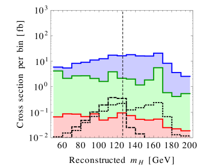
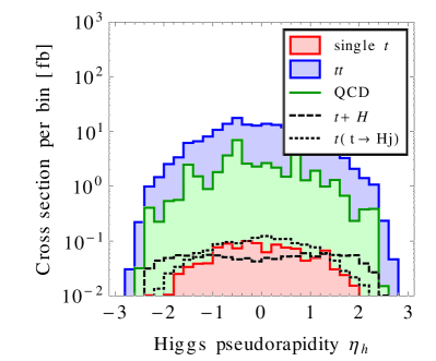
After top tagging and Higgs tagging, we preselect events by requiring that at least one fat jet in the event carries a Higgs tag and at least one of the remaining fat jets carries a top tag. We define the Higgs candidate as the hardest Higgs-tagged fat jet and the top candidate as the hardest top-tagged fat jet different from the Higgs candidate. If the hardest Higgs-tagged fat jet is the only fat jet carrying a top tag, we take it to be the top candidate and use the next-to-hardest Higgs-tagged fat jet as the Higgs candidate. Event counts after preselection are given in Table 5, and the distributions of two important kinematic quantities—the invariant mass and the pseudorapidity of the Higgs candidate—are shown in Fig. 7 for . As expected, peaks around the true value of the Higgs mass for the signal, while showing no distinct features for the background. The forward bias of the distribution for signal events is again related to angular momentum conservation in the center of mass frame and the net boost of that frame in the direction of the incoming up quark in the process (see Sec. 2 for details), making again a good discriminant between and couplings. The and distributions shown in Fig. 7 suggest the final cuts and . We see from the predicted event counts in the last row of Table 5 that the signal-to-background ratio is substantially improved by these cuts. Even though the signal-to-square root background ratio is similar before and after the final cuts, this improvement makes the search much more robust with respect to systematic uncertainties.
From the event counts in Table 5 and the projected sensitivities in Table 6, we see that analysis 2 outperforms analysis 1 in the case of couplings, but is not competitive for couplings, as expected. It could therefore be an important ingredient in a multi-channel search for couplings, and an important cross check in case a signal is found in a different channel.
5 Discussion and Conclusions
In this work we have investigated the sensitivity of the LHC to flavor violating top–Higgs interactions. Since these interactions are highly suppressed in the SM, a positive signal at the LHC would constitute a clear sign of new physics, for instance in the form of additional Higgs bosons or nonrenormalizable couplings of the Higgs.
While exiting experimental searches have mainly concentrated on anomalous top decays , we have shown that anomalous single top plus Higgs production is almost as important in the case of couplings and therefore offers a promising avenue for further improvements in the sensitivity. Single top + Higgs production is less relevant for probing interactions due to the suppressed charm quark parton distribution in the proton.
In Sec. 3, we have recast existing searches for multilepton [9], diphoton + lepton [2] and vector boson + Higgs [12] final states to derive improved limits on couplings, including the contribution form single top + Higgs production. Our best limits on the branching ratio and the Yukawa couplings come from the diphoton plus leptons final state and are a factor 1.5 stronger than the previously derived limits on and . Limits from multileptons and vector boson + Higgs searches are slightly weaker, but still competitive. Our new limits are summarized in the upper part of Table 7.
| New limits from existing data | ||||
|---|---|---|---|---|
| Sec. 3.1: Multilepton | ||||
| Sec. 3.2: Diphoton plus lepton | ||||
| Sec. 3.3: Vector boson plus Higgs | ||||
| Projected future limits (13 TeV, 100 fb-1) | ||||
| Sec. 3.3: Vector boson plus Higgs | ||||
| Sec. 4.1: Multilepton | ||||
| Sec. 4.2: Fully hadronic | ||||
In the second part of the paper, Sec. 4, we have investigated possible future improvements of searches for flavor violating top–Higgs couplings, including the development of a completely new search strategy in fully hadronic final states. We have shown that multilepton, diphoton + lepton and vector boson + Higgs searches can substantially improve the current bounds and may have the potential to distinguish couplings from couplings at the level once a signal is discovered at . This is possible because, in the case of couplings, the process contributes significantly to the signal. In this process, the Higgs boson tends to be produced with a large forward boost, while in all other signal processes the Higgs rapidity distribution is more central. Moreover, leads to an asymmetry of the total charge of the final state leptons. For couplings, the corresponding process is suppressed by the parton distribution function of the charm quark and is therefore negligible.
Regarding the fully hadronic processes and , we have developed an analysis using jet substructure techniques to tag SM top decays, decays and decays. We find that backgrounds can be suppressed efficiently in such a search, leading to a sensitivity that is competitive to that of searches with leptonic or semileptonic final states. Our projected future limits are summarized in the lower part of Table 7.
For completeness we note that several other LHC processes exhibit potential sensitivity to flavor violating top–Higgs interactions. For example, couplings can lead to an enhancement of di-Higgs production at tree level through – collisions with -channel top exchange. However, in this case the relevant cross-section scales with the fourth power of the flavor violating Yukawa couplings, and at the current upper limit the resulting effect is already subleading compared to the (already very suppressed) SM rate [45].333Using FeynArts and FormCalc [46], we have also checked that possible loop contributions to gluon fusion induced di-Higgs production [47] are negligible given current constraints on these couplings. Similarly, same-sign top production from – scattering via Higgs exchange in the -channel is expected to be below the current experimental sensitivity (cf. [48]) given currently allowed values of .
To summarize, several signatures of flavor violating interactions at the LHC which we have studied in the present paper exhibit comparable prospects to constrain or discover such phenomena. Moreover, it may be possible to even discriminate between and signals by exploiting the presence of absence of the partonic process . When multiple searches are combined into a global analysis, they could allow the LHC experiments to probe the flavor violating top–Higgs interactions well into the region of .
Acknowledgements
We would like to thank Yan Wang for sharing the results on the NLO QCD corrections to associated top plus Higgs production. We also thank Tilman Plehn, Torben Schell and Peter Schichtel for very useful discussions. AG would like to thank Luka Leskovec for his help with computing facilities used in this work. JK acknowledges the hospitality of CERN and of the Aspen Center for Physics (supported by the US National Science Foundation under Grant No. 1066293), where part of this work has been carried out. This work was supported in part by the Slovenian Research Agency.
Appendix A Tagging Top Decays to Higgs + Jet
In this appendix, we give details on the “” tagging algorithm used in Sec. 4.2 to identify hadronic events. Our method is based on the HEPTopTagger algorithm v1.0 [34, 35], a detailed description of which is given in the Appendix of [35]. In simplified terms HEPTopTagger starts from a fat jet, which it unclusters partially to identify the three subjets that are most likely to originate from a top decay based on their invariant mass . The algorithm then imposes cuts on the invariant masses , and of different pairings of these three subjets, where the indices 1, 2 and 3 stand for the subjet with the largest, next-to-largest and smallest , respectively. In particular, one of the following three conditions has to be satisfied [35]:
| (11) |
The motivation for these cuts can be seen in Fig. 8, which shows the distributions of and for signal and background events. The conditions on the left in Eq. (11) loosely define the physically accessible region, while the cuts on the right impose the condition that one of the subjet pairs reconstructs to the mass of an on-shell intermediate particle: the for the original HEPTopTagger and the Higgs for our tagger. Based on Fig. 8, we choose , in our most conservative analysis (loose tags), and , in our more optimistic analysis (tight tags).444Note that a tight tag implies not only more restrictive cuts on and , but also that the fat jet does not simultaneously carry a top tag. The latter is based on the observation that the invariant masses of the subjets from Higgs decay tend to be slightly smaller than the true on average. We attribute this to individual hadrons falling outside the fat jet cone, being reconstructed as part of the wrong subjet, or being removed by filtering. Note that these effects are largest for the softest subjets.
 |
 |
 |
| (a) | (b) | (c) |
As discussed in Sec. 4.2, we require the two jets most likely originating from a Higgs decay to contain tags. In the absence of a full detector simulation we perform tagging by searching for or quarks with GeV within an angular distance from the reconstructed subjet axis. If a or quark satisfying these requirements exists inside the subjet, we assign a tag with a probability depending on the quark’s transverse momentum and its pseudorapidity according to
| (12) | ||||
| (13) |
If no sufficiently hard and central or quark is found, the probability that the jet is still misidentified as a jet is . In practice, we do not actually discard events, but merely reweight them with the appropriate tagging efficiency.
References
- Harnik et al. [2013] R. Harnik, J. Kopp, and J. Zupan, JHEP 1303, 026 (2013), 1209.1397.
- CMS Collaboration [2014] CMS Collaboration (2014), CMS-PAS-HIG-13-034.
- Aguilar-Saavedra and Branco [2000] J. Aguilar-Saavedra and G. Branco, Phys.Lett. B495, 347 (2000), hep-ph/0004190.
- Craig et al. [2012] N. Craig, J. A. Evans, R. Gray, M. Park, S. Somalwar, et al., Phys.Rev. D86, 075002 (2012), 1207.6794.
- Wang et al. [2012] Y. Wang, F. P. Huang, C. S. Li, B. H. Li, D. Y. Shao, et al., Phys.Rev. D86, 094014 (2012), 1208.2902.
- Chen et al. [2013] K.-F. Chen, W.-S. Hou, C. Kao, and M. Kohda, Phys.Lett. B725, 378 (2013), 1304.8037.
- Atwood et al. [2013] D. Atwood, S. K. Gupta, and A. Soni (2013), 1305.2427.
- Agrawal et al. [2013] P. Agrawal, S. Bandyopadhyay, and S. P. Das, Phys.Rev. D88, 093008 (2013), 1308.3043.
- CMS Collaboration [2013a] CMS Collaboration (2013a), CMS-PAS-SUS-13-002.
- ATLAS Collaboration [2013a] ATLAS Collaboration (2013a), ATLAS-CONF-2013-081, ATLAS-COM-CONF-2013-090.
- Aad et al. [2014] G. Aad et al. (ATLAS Collaboration) (2014), 1403.6293.
- CMS Collaboration [2013b] CMS Collaboration (2013b), CMS-PAS-HIG-12-053.
- Li et al. [1991] C. S. Li, R. J. Oakes, and T. C. Yuan, Phys.Rev. D43, 3759 (1991).
- Drobnak et al. [2010] J. Drobnak, S. Fajfer, and J. F. Kamenik, Phys.Rev.Lett. 104, 252001 (2010), 1004.0620.
- Zhang and Maltoni [2013] C. Zhang and F. Maltoni, Phys.Rev. D88, 054005 (2013), 1305.7386.
- Czakon et al. [2013] M. Czakon, P. Fiedler, and A. Mitov, Phys.Rev.Lett. 110, 252004 (2013), 1303.6254.
- Martin et al. [2009] A. Martin, W. Stirling, R. Thorne, and G. Watt, Eur.Phys.J. C63, 189 (2009), 0901.0002.
- [18] Y. Wang, private communication.
- Christensen and Duhr [2009] N. D. Christensen and C. Duhr, Comput.Phys.Commun. 180, 1614 (2009), 0806.4194.
- Alwall et al. [2011] J. Alwall, M. Herquet, F. Maltoni, O. Mattelaer, and T. Stelzer, JHEP 1106, 128 (2011), 1106.0522.
- Sjostrand et al. [2006] T. Sjostrand, S. Mrenna, and P. Z. Skands, JHEP 0605, 026 (2006), hep-ph/0603175.
- de Favereau et al. [2014] J. de Favereau et al. (DELPHES 3), JHEP 1402, 057 (2014), 1307.6346.
- Heinemeyer et al. [2013] S. Heinemeyer et al. (LHC Higgs Cross Section Working Group) (2013), 1307.1347.
- Meade and Reece [2007] P. Meade and M. Reece (2007), hep-ph/0703031.
- Read [2002] A. L. Read, J.Phys. G28, 2693 (2002).
- CMS Collaboration [2013c] CMS Collaboration (2013c), CMS-PAS-HIG-13-025.
- https://feynrules.irmp.ucl.ac.be/wiki/HiggsEffectiveTheory [2011] https://feynrules.irmp.ucl.ac.be/wiki/HiggsEffectiveTheory (2011).
- ATLAS Collaboration [2013b] ATLAS Collaboration (2013b), ATL-PHYS-PUB-2013-012.
- Jadach et al. [1993] S. Jadach, Z. Was, R. Decker, and J. H. Kuhn, Comput.Phys.Commun. 76, 361 (1993).
- CMS Collaboration [2012] CMS Collaboration, JINST 7, P01001 (2012), 1109.6034.
- Khatibi and Najafabadi [2014] S. Khatibi and M. M. Najafabadi (2014), 1402.3073.
- Farina et al. [2013] M. Farina, C. Grojean, F. Maltoni, E. Salvioni, and A. Thamm, JHEP 1305, 022 (2013), 1211.3736.
- Kaplan et al. [2008] D. E. Kaplan, K. Rehermann, M. D. Schwartz, and B. Tweedie, Phys.Rev.Lett. 101, 142001 (2008), 0806.0848.
- Plehn et al. [2010a] T. Plehn, G. P. Salam, and M. Spannowsky, Phys.Rev.Lett. 104, 111801 (2010a), 0910.5472.
- Plehn et al. [2010b] T. Plehn, M. Spannowsky, M. Takeuchi, and D. Zerwas, JHEP 1010, 078 (2010b), 1006.2833.
- Dokshitzer et al. [1997] Y. L. Dokshitzer, G. Leder, S. Moretti, and B. Webber, JHEP 9708, 001 (1997), hep-ph/9707323.
- Cacciari et al. [2012] M. Cacciari, G. P. Salam, and G. Soyez, Eur.Phys.J. C72, 1896 (2012), 1111.6097.
- Gleisberg et al. [2009] T. Gleisberg, S. Hoeche, F. Krauss, M. Schonherr, S. Schumann, et al., JHEP 0902, 007 (2009), 0811.4622.
- Schumann and Krauss [2008] S. Schumann and F. Krauss, JHEP 0803, 038 (2008), 0709.1027.
- Gleisberg and Hoeche [2008] T. Gleisberg and S. Hoeche, JHEP 0812, 039 (2008), 0808.3674.
- Hoeche et al. [2009] S. Hoeche, F. Krauss, S. Schumann, and F. Siegert, JHEP 0905, 053 (2009), 0903.1219.
- Schonherr and Krauss [2008] M. Schonherr and F. Krauss, JHEP 0812, 018 (2008), 0810.5071.
- Aad et al. [2011] G. Aad et al. (ATLAS Collaboration), Eur.Phys.J. C71, 1763 (2011), 1107.2092.
- Butterworth et al. [2008] J. M. Butterworth, A. R. Davison, M. Rubin, and G. P. Salam, Phys.Rev.Lett. 100, 242001 (2008), 0802.2470.
- Baglio et al. [2013] J. Baglio, A. Djouadi, R. Gr ber, M. M hlleitner, J. Quevillon, et al., JHEP 1304, 151 (2013), 1212.5581.
- Hahn [2000] T. Hahn, Nucl.Phys.Proc.Suppl. 89, 231 (2000), hep-ph/0005029.
- Djouadi et al. [1999] A. Djouadi, W. Kilian, M. Muhlleitner, and P. Zerwas, Eur.Phys.J. C10, 45 (1999), hep-ph/9904287.
- ATLAS Collaboration [2012] ATLAS Collaboration (2012), ATLAS-CONF-2012-130, ATLAS-COM-CONF-2012-163.