Stop Reconstruction with Tagged Tops

Abstract

At the LHC combinatorics make it unlikely that we will be able to observe stop pair production with a decay to a semi-leptonic top pair and missing energy for generic supersymmetric mass spectra. Using a Standard-Model top tagger on fully hadronic top decays we can not only extract the stop signal but also measure the top momentum. To illustrate the promise of tagging tops with moderate boost we include a detailed discussion of our HEPTopTagger algorithm.

I Introduction

Searches for top squarks at hadron colliders aim at a fundamental questions of electroweak symmetry breaking — if the Higgs boson should be a fundamental scalar, how can its mass be stabilized? In particular, is the Higgs mass protected by some symmetry? Such symmetries typically predict the existence of a top partner, like in supersymmetric or little Higgs models review ; meade . In such a case, studying the properties of top partners allows us to unravel the nature of such an underlying fundamental symmetry protecting the fundamental Higgs mass at the scale of electroweak symmetry breaking.

At the Tevatron, low-mass stop searches look for loop-induced stop decays stop_decays to charm quarks and the lightest neutralino stops_tevatron_c . Increasing the stop mass makes it more promising to look for decays to a bottom jet and the lightest chargino stops_tevatron_b , a final state irreducible from a leptonic top decay. Finally, if the stop becomes heavier and the strong decay in a top quark and a gluino is not yet kinematically allowed, the stop can decay into a top quark and the lightest neutralino stop_decays . This final state has the advantage that at least hadronic top quarks we might be able to fully reconstruct, which puts us into a promising position to study angular correlations in the stop pair final state. Fully hadronic top pairs from stop production are studied in the CMS TDR cms_tdr , Section 13.12, but with the requirement of an additional lepton pair from the stop decays. Including this lepton essentially removes all QCD backgrounds. In this analysis we will show that such a lepton is not needed once we apply an efficient identification of boosted tops.

There have been several suggestions as to what we might be able to say about the nature of the stop based on a momentum reconstruction of its visible decay products stops_measure ; weiler ; however, to date there exists no experimentally confirmed analysis which extracts hadronic or semi-leptonic top pairs plus missing energy at the LHC. This means that without a viable discovery channel all of those suggestions are bound to end up pure fiction in the era of actual LHC data. In this paper we will first convince ourselves that in spite of claims to the contrary there is no reason to assume that stop decays to semi-leptonic top quarks plus missing energy will be discovered at the LHC — in line with the state of the art of experimental simulations. We will then study the reach of fat-jet fatjet_vh ; david_e ; fatjet_tth searches for purely hadronic stop decays and their potential when it comes to reconstructing for example the top momenta. In the Appendix we will give a long-overdue study of a hadronic top tagger based on the Cambridge/Aachen jet algorithm and a mass drop criterion. This HEPTopTagger (Heidelberg–Eugene–Paris) is designed to cover moderately boosted top quarks, as we also expect them for Standard Model processes at the LHC fatjet_tth . 

II Standard Semi-Leptonic Analysis

Using semi-leptonic top decays to extract the signature

$$pp\to\tilde{t}_{1}\tilde{t}_{1}^{*}\to(t\tilde{\chi}_{1}^{0})\,(\bar{t}\tilde{\chi}_{1}^{0})\to(b\ell^{+}\nu\tilde{\chi}_{1}^{0})\,(\bar{b}jj\tilde{\chi}_{1}^{0})+(bjj\tilde{\chi}_{1}^{0})\,(\bar{b}\ell^{-}\bar{\nu}\tilde{\chi}_{1}^{0})$$ (1)

including four jets and missing energy from the irreducible top pair production requires a detailed analysis of the two-dimensional missing energy vector and its correlation with the visible momenta in the final state. The stop mass we assume to be 340 GeV weiler , decaying with essentially 100% branching ratio to a top quark and a 98 GeV lightest neutralino. The leading-order production rate for stop pairs according to Pythia is around 3.2 pb, the next-to-leading order rate from Prospino is 5.1 pb prospino . To compare our result to the original analysis, in this section we do not apply the NLO corrections, i.e.  a flat $K$ factor of 1.59. For the same reason we normalize our top-pair sample to 550 pb instead of the approximate NNLO rate around 918 pb top_rate , corresponding to $K=1.67$. The original semi-leptonic analysis starts from a set of acceptance cuts requiring exactly four jets and a charged lepton weiler :

$$p_{T,j} >25~{}{\rm GeV}\qquad\qquad\qquad |\eta_{j}| <4.0\qquad\qquad\qquad \Delta R_{jj} >0.4$$

$$p_{T,\ell} >20~{}{\rm GeV} |\eta_{\ell}| <2.5 \Delta R_{j\ell} >0.4\;.$$ (2)

The top-pair and $W$+jets backgrounds can be reduced by an additional set of cuts, largely inspired by the usual semi-leptonic top analyses at the Tevatron. One of the four jets should be $b$-tagged, with the appropriate efficiency of $60\%$. The different jets, the lepton and the missing energy vector have to be separated according to weiler

$$\text{min}_{j}\Delta R_{\ell j} <1.5\qquad\qquad\qquad \hbox to0.0pt{\hbox to5.03125pt{\hfil/\hfil}\hss}p_{T} >125~{}{\rm GeV}$$

$$\cos\phi(p_{T,\ell},\hbox to0.0pt{\hbox to6.5382pt{\hfil/\hfil}\hss}\vec{p}_{T}) >0.7 0.8 <\text{min}_{x}\Delta\phi(\hbox to0.0pt{\hbox to6.5382pt{\hfil/\hfil}\hss}\vec{p}_{T},x)<1.3\quad(x=\ell,j)\;,$$ (3)

and the two reconstructed top decays have to be fulfilled weiler

$$|m_{t}^{\text{rec}}-m_{t}| <5~{}{\rm GeV}\qquad$$ (hadronic top)

$$|m_{W}^{\text{rec}}-m_{W}| >40~{}{\rm GeV}\qquad \text{(leptonic top veto with $m_{t}$ constraint for $\vec{p}_{\nu L}$~{}\cite[cite]{\@@bibref{Authors Phrase1YearPhrase2}{top_rec_semilep}{\@@citephrase{(}}{\@@citephrase{)}}})}\;.$$ (4)

The first condition identifies the hadronically decaying top while the second condition makes sure that once we include the entire missing energy from the leptonic top decay and the pair of neutralinos the mass of the reconstructed top candidate does not match the physical top mass weiler . It is possible to improve the leptonic top veto for example by solving the kinematical constraints for the top mass and requiring that this complex solution have the correct real part as well as a vanishing imaginary part top_rec_semilep . However, these details should not affect the final outcome of our analysis, as we will see from the discussion. In the following, this analysis setup we refer to as ‘PW’ weiler .

We simulate signal and background using Herwig herwig , Pythia pythia and Alpgen-Pythia alpgen including initial and final state radiation, hadronization and underlying event. The top and stop samples we generate inclusively without restricted decays. For the fast detector simulation we rely on Acerdet acerdet , a reasonably reliable fast simulation of LHC detectors which should agree well with full detector simulation for the analysis presented here csc_notes . The final results including the three leading backgrounds we show in Table 1, labelled ‘PW’ weiler . Compared to the original work in Ref. weiler we see that the signal efficiency is considerable lower, which is largely due to combinatorics in the reconstruction of the hadronic top and subsequent reconstruction hypotheses. In the next section, this will serve as the motivation to instead use a top tagger, which we know is best suited to automatically resolve combinatorial issues fatjet_tth .

Given our results we can slightly optimize the original semi-leptonic analysis: Instead of exactly four jets, we require a minimum of four jets to allow for example for initial state radiation. The $b$ tag we apply to jets with $|\eta_{j}|<2.5$. Finally, the hadronic mass reconstruction is considered successful if the three-jet invariant mass is within 15 GeV of the nominal top quark mass, instead of 5 GeV. Again, the results are shown in Table 1, labelled ‘PSTZ’. For large stop masses we could consider applying a significantly stiffer cut on missing energy, but as we will discuss in the next section such a cut will leave us with essentially unknown detector fake rates.

	$\sigma$ [pb]	$N_{\text{simulated}}$	$\epsilon_{\text{PW}}$	$\epsilon_{\text{PSTZ}}$	$\sigma\cdot\epsilon_{\text{PW}}$ [fb]	$\sigma\cdot\epsilon_{\text{PSTZ}}$ [fb]	Ref. weiler
$\tilde{t}_{1}\tilde{t}_{1}^{*}$	3.2	120000	$(1.5\pm 0.1)\cdot 10^{-3}$	$(1.2\pm 0.03)\cdot 10^{-2}$	4.8	38	56
$t\bar{t}$	550	500000	$(8.6\pm 1.3)\cdot 10^{-5}$	$(4.3\pm 0.3)\cdot 10^{-4}$	47.3	237	20
$W+4j$	56.5	397698	$(3.5\pm 0.9)\cdot 10^{-5}$	$(3.8\pm 0.3)\cdot 10^{-4}$	2.0	21.5	$\sim 2.7$
$W+bbjj$	0.63	761937	$(3.1\pm 0.2)\cdot 10^{-4}$	$(2.7\pm 0.06)\cdot 10^{-3}$	0.2	1.7	$\sim 1.5$
SM total					49.5	260.2	$\sim 24.2$
$S/B$					0.096	0.15	2.3
$S/\sqrt{B}_{10~{}{\rm fb^{-1}}}$					2.2	7.5	36

Table 1: Signal and backgrounds for the semi-leptonic stop analysis. The three sets of results correspond to the analysis suggested in Ref. weiler including ISR/FSR, hadronization and fast detector simulation (PW), a slightly modified version of the same analysis including ISR/FSR, hadronization and fast detector simulation (PSTZ), and the numbers from Ref. weiler adjusted for all electron and muon final states, without ISR/FSR or hadronization or a complete fast detector simulation. All rates are given at leading order, to allow for a comparison with the original numbers in the last column.

The key observable shown in Table 1 is the signal-to-background ratio $S/B$, which determines how well we need to know the theory and the systematics of the QCD backgrounds to extract the signal. Note that none of the analyses shown offers a clear side-bin background normalization. While the optimized analysis has an increased signal efficiency by almost a factor ten and a promising Gaussian statistical significance of $S/\sqrt{B}=7.5$ (for $10~{}{\rm fb^{-1}}$), values around $S/B\sim 1/7$ are clearly insufficient to convincingly extract the stop signal in the presence of systematic and theory errors.

The background results in Table 1 should still be taken with a grain of salt. While our signal efficiencies are in good agreement between Pythia and Herwig (Fortran and C++), the background numbers are sensitive to the underlying event. We can check this effect by turning on/off the multi-parton interactions in Herwig++, which leads to a decrease of the background rejection by an order of magnitude. However, this does not affect the conclusion of this section, namely that semi-leptonic stop searches are very unlikely to be visible at the LHC. This is a generic statement in the sense that looking at the systematic uncertainties we need to overcome a relative factor of $\mathcal{O}(200)$ between the stop signal and the top background rates and to our knowledge there is no kinematic cut which for generic mass spectra significantly improves this ratio after including detector smearing and fakes ayres .

III Hadronic Fat-Jet Analysis

Given that the semi-leptonic analysis shown in the last section is unlikely to work at all, an alternative strategy would be to search for stop pairs in purely hadronic top decays. Those would allow us to fully reconstruct the final state and analyze the angular correlation in detail:

$$pp\to\tilde{t}_{1}\tilde{t}_{1}^{*}\to(t\tilde{\chi}_{1}^{0})\,(\bar{t}\tilde{\chi}_{1}^{0})\to(bjj\tilde{\chi}_{1}^{0})\,(\bar{b}jj\tilde{\chi}_{1}^{0})\;.$$ (5)

Our hadronic stop analysis is based on two tagged hadronic top quarks, using the algorithm described in the Appendix. Tagging $W$ bosons in their decays to geometrically large jets fatjet_w has been around in the LHC literature for quite a while, including its applications in searches for supersymmetry fatjet_susy . Higgs tags can be implemented in a similar manner, and as it turns out they show the best performance fatjet_vh ; fatjet_tth ; fatjet_susy ; fatjet_higgs when based on the purely geometric C/A jet algorithm ca_algo ; fastjet . Inspired by searches for very heavy resonances decaying to top pairs tt_resonance several top taggers have been developed, again in the same spirit, but based on different jet algorithms as well as on jet shapes top_tag ; david_e ; fatjet_tth ; fatjet_wash . One disadvantage of most of these top taggers is that they are not designed to work for the kind of transverse momenta we can expect in Standard Model processes. This means that unlike the $W$ and Higgs taggers fatjet_vh ; giacinto , top taggers might be very hard to establish experimentally. Following the $t\bar{t}H$ analysis fatjet_tth we slightly refine our top tagger for moderate top boosts and apply it to this new challenge: extract a new-physics signal from purely hadronic final states and reconstruct its kinematics.

For triggering we expect our signal events to pass the jets plus missing energy trigger at the LHC. To extract it from the backgrounds we can employ the recently developed fat-jet tools which aim at tagging a boosted top jet without being killed for example by combinatorics. We start by constructing jets using the Cambridge/Aachen algorithm ca_algo , implemented in Fastjet fastjet , with $R=1.5$ and requiring at least two jets with

$$p_{T,j}>200/200~{}{\rm GeV}\qquad\qquad\qquad\qquad\hbox to0.0pt{\hbox to5.03125pt{\hfil/\hfil}\hss}p_{T}>150~{}{\rm GeV}\;.$$ (6)

Those two cuts are chosen to obtain the largest signal-to-background ratio $S/B$. To reduce the probability of fake missing energy due to detector effects we require the two-dimensional missing energy vector to be well separated from the jets, to avoid cases where missing energy is generated by just mis-measuring one jet. This should leave us with a suppression factor of 1% for fake missing energy above $\hbox to0.0pt{\hbox to5.03125pt{\hfil/\hfil}\hss}p_{T}>150$ GeV in QCD jet events without any physical missing energy csc_notes , which we apply in the following. Next, we veto isolated leptons with $p_{T,\ell}>15$ GeV, $|\eta_{\ell}|<2.5$, requiring $E_{T}^{\text{had}}<0.1E_{T}^{\text{lep}}$ within $R<0.3$ around the lepton.

At this level we apply the top tagger described later and in the Appendix and require two tops to be identified and reconstructed. Finally, after requiring one $b$ tag inside the first tagged top we construct $m_{T2}$ mt2 . Assuming we do not know the LSP mass, i.e.  setting it to zero in the $m_{T2}$ construction, we require

$$m_{T2}>250~{}{\rm GeV}\;.$$ (7)

While in Table 2 we will see that this cut has hardly any impact on the signal significance $S/\sqrt{B}$, at least for small stop masses, we apply it to increase the signal-to-background ratio $S/B$ and hence become less sensitive to systematic and theory errors.

Constructing the $m_{T2}$ distributions has two motivations, of which the background rejection cut might even be the lesser. From the two panels of Figure 1 we see that $m_{T2}$ with an assumed massless LSP is better suited to distinguish the stop signal from the top background. As expected, Figure 1 also shows that for larger stop masses this cut becomes increasingly effective. More importantly, once we know the correct value of $m_{\tilde{\chi}^{0}_{1}}$ we can determine the stop mass from the endpoint of the $m_{T2}$ distribution. Determining the uncertainties of such a mass measurement, however, is beyond the scope of our phenomenological analysis. Obviously, due to the wrong decay topology the endpoint of the $t\bar{t}$ background has nothing to do with the physical top mass, so we cannot use it to gauge the stop mass measurement.

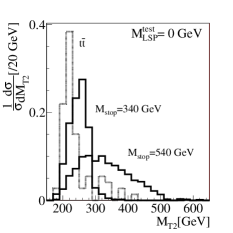
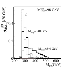
Figure 1: Normalized $m_{T2}$ distributions for the stop signal ($m_{\tilde{t}}=340$ GeV) and the $t\bar{t}$ background, after reconstructing two (real of fake) hadronic top quarks. The hypothetical LSP mass we set to $m_{\tilde{\chi}^{0}_{1}}=0$ GeV (left) or to the correct value of $m_{\tilde{\chi}^{0}_{1}}=98$ GeV (right).

For a double Standard Model top tag the mis-tagging probability when applied to a pure QCD or $W$+jets sample after our process specific cuts turns out to be (not much) below 0.1%, comparable to the numbers quoted in the Appendix, Table 3. From the first column of Table 2 it is clear that such a reduction rate is not sufficient. Therefore, we follow the example of the Higgs tagger fatjet_vh ; fatjet_tth and apply an additional $b$ tag inside the main constituents of the first tagged top. Limiting this $b$ tag to the three main constituents of one specific tagged top reduces the fake rate in particular from charm jets or gluons splitting into $b\bar{b}$ pairs. Assuming a 60% tagging efficiency and a light-flavor rejection around 1/50 this will give the first top tag a mistag rate well below 0.1%. As it will turn out, this is sufficient to render the QCD and $W$+jets backgrounds negligible compared to the $t\bar{t}$ background. Charm jets in the QCD jets sample we do not expect to be a problem. On the one hand, they have a 10% mis-tagging probability for our $b$ tag, but on the other hand the will appear much less frequently, based for example on the reduced probability of gluon jets splitting into quarks — a factor 1/4 from counting quark flavors in $g\to q\bar{q}$ alone. Last but not least, given the moderate boost of the top quarks we check that including a $(0.1,0.1)$ granularity of the detector in a lego plot has no impact on our analysis.

The large transverse momentum of the two candidate fat jets in Eq.(6) allows us not to worry about triggering on the one hand and to generate events with a sizeable efficiency — for the actual analysis this cut has little effect, because inside the top tagger we apply a lower cut on the transverse momentum of the reconstructed top $p_{T,t}^{\text{rec}}>200$ GeV. We explicitly check this by lowering the acceptance cuts to $p_{T,j}>100$ GeV and find no effect on the final numbers of the analysis.

The different steps of our analysis are illustrated in Table 2, for different stop masses and the leading backgrounds. The event numbers are normalized to NLO cross sections for the stop pair signal and the leading $t\bar{t}$ background. For QCD and $W$+jets the normalization after cuts has many sources of mostly experimental uncertainty that we can as well stick to the leading order normalization.

Stop pair signal — in contrast to for example Higgs signals strongly interacting new particles will be produced with sizeable rates at the LHC. For identical masses, the production rate for stop pairs is actually the smallest of all QCD-initiated supersymmetric processes, due to the large number of essentially degenerate light-flavor squarks at the LHC, the fundamental color charge of the stops, and the lack of a $t$-channel $q\bar{q}$ production process. Typical NLO cross sections for stop pair production range from 5.1 pb ($m_{\tilde{t}}=340$ GeV) to 0.4 pb (540 GeV) and 0.15 pb (640 GeV) prospino . After requiring missing energy, two top tags and one $b$ tags we are left with several fb of rate. As we can see in Figure 1 the stiff $m_{T2}$ cut is not particularly efficient, in particular for small stop masses, but it does give us the necessary handle to suppress the $t\bar{t}$ background to a level of $S/B\sim\mathcal{O}(1)$.

Top pair background — as we know from the semi-leptonic analysis and as we can see in Table 2, top pair production is the most dangerous background to stop searches. Its total rate shows a relative enhancement of several hundred over the signal and two physical tops can be tagged including the $b$ jet we are requiring. Purely hadronic top decays are reduced by our missing energy cut in analogy to the pure QCD background, i.e.  by a factor 1/100. Semi-leptonic top decays are more dangerous, since after one top tag the discussion in the Appendix shows that there is very likely a second top tag based on recoiling QCD jets. After two top tags the $t\bar{t}$ background is still larger than the signal. Therefore, we apply a cut on $m_{T2}$, clearly distinguishing missing energy from two LSPs to large missing energy from one neutrino in the semi-leptonic top background.

QCD background — just because of its sheer size QCD jet production tends to be an unsurmountable background at the LHC. After requiring two hard jets we are still left with more than $10^{7}~{}{\rm fb}$ of rate. As discussed in the Appendix we cannot suppress such a rate only using the kinematic features of the top decay. The probabilistic treatment of fake missing energy (1/100) and one $b$ mis-tag (1/50) give us an additional suppression, where after two top tags we arrive below the $t\bar{t}$ background. Note that we cannot assign a $m_{T2}$ survival probability to the QCD background, since we do not know the distribution of the detector-fake missing energy vector. However, because this fake missing energy will be uncorrelated with the other momenta in the event, just like one additional missing particle, we estimate the efficiency by the $t\bar{t}$ value around 22%. If for some reason QCD jet production should still pose an experimental problem there is the option of requiring a $b$ tag also in the second reconstructed top jet.

$W$+jets background — in contrast to QCD jets production this process includes actual missing energy. Technically, we simulate this background using Alpgen alpgen with four hard jets plus additional collinear jet radiation. The $W$+jets rate only exceeds the signal rate by less than a factor 100, so applying the basic cuts and requiring two tagged top quarks reduces it to a level we can deal with. The $b$ tag and the additional cut on $m_{T2}$ reduce the $W$+jets background to a level where it is hard to predict without sufficient statistics. Irrespective of the details we can conclude that $W$+jets do not pose a problem to the stop pair search.

$Z$+jets background — because of the significantly smaller rate, the slightly lower invisible $Z$ branching ratio and the sizeable probability to miss the lepton from the $W$ decay we can safely assume that the $Z$+jets background will be as irrelevant as the $W$+jets background after cuts. Numerically, even with too low statistics for a detailed analysis we see that after cuts the $(Z\to\nu\nu)$+jets background is always smaller than the $W$+jets background by a factor $\mathcal{O}(1/3)$ and hence irrelevant.

	$\tilde{t}_{1}\tilde{t}_{1}^{*}$						$t\bar{t}$	QCD	$W$+jets	$Z$+jets	$S/B$	$S/\sqrt{B}_{10~{}{\rm fb^{-1}}}$
$m_{\tilde{t}}[{\rm GeV}]$	340	390	440	490	540	640					340
$p_{T,j}>200$ GeV, $\ell$ veto	728	447	292	187	124	46	87850	$2.4\cdot 10^{7}$	$1.6\cdot 10^{5}$	n/a	$3.0\cdot 10^{-5}$
$\hbox to0.0pt{\hbox to5.03125pt{\hfil/\hfil}\hss}p_{T}>150$ GeV	283	234	184	133	93	35	2245	$2.4\cdot 10^{5}$	1710	2240	$1.2\cdot 10^{-3}$
first top tag	100	91	75	57	42	15	743	7590	90	114	$1.2\cdot 10^{-2}$
second top tag	15	12.4	11	8.4	6.3	2.3	32	129	5.7	1.4	$8.3\cdot 10^{-2}$
$b$ tag	8.7	7.4	6.3	5.0	3.8	1.4	19	2.6	$\lesssim 0.2$	$\lesssim 0.05$	0.40	5.9
$m_{T2}>250$ GeV	4.3	5.0	4.9	4.2	3.2	1.2	4.2	$\lesssim 0.6$	$\lesssim 0.1$	$\lesssim 0.03$	0.88	6.1

Table 2: Signal (for different stop masses) and backgrounds for the hadronic fat-jet analysis. All numbers given in fb, the significance is computed for $10~{}{\rm fb^{-1}}$. The $\tilde{t}_{1}\tilde{t}_{1}^{*}$ and $t\bar{t}$ rates are normalized to their higher-order values top_rate ; prospino . $Z$+jets we simulate with the neutrino decay specified.

The right columns of Table 2 clearly show that extracting hadronic stop pairs from the different Standard Model backgrounds will not be a problem at all. The statistical significance is above the discovery limit already with an integrated luminosity of $10~{}{\rm fb^{-1}}$. The event numbers are not huge, but a more careful statistical treatment for example of our crude $m_{T2}$ cut will change this easily. In contrast to semi-leptonic stop decays systematics will not pose any problem either, possible complications from jet combinatorics should be automatically resolved by the top tagger fatjet_tth .

One curious feature we see once we increase the stop mass: for a constant LSP mass the increase in the cut efficiencies actually over-compensates the decrease in the stop production rate. This is most obvious for the $m_{T2}$ cut shown in Figure 1, but it also holds for example for the top tagging efficiency which benefits from the increased stop-neutralino mass difference. Table 2 therefore does not give a good estimate of the stop mass reach. To answer this question we would need to adjust the $\hbox to0.0pt{\hbox to5.03125pt{\hfil/\hfil}\hss}p_{T}$ and $m_{T2}$ cuts which as it stands are optimized for 340 GeV stops.

Moreover, it is clear that from the endpoints of the $m_{T2}$ distributions we should be able to measure the stop mass (or better the stop–neutralino mass difference) in this process. While making this quantitative statement does not require any further work, actually estimating the experimental error on stop mass measurements using fat jets goes far beyond what we can do in this paper. We therefore refrain from quoting any number for the stop mass measurements and leave it at this statement and the encouragement for a detailed experimental analysis including full detector simulation. For supersymmetric parameter analyses such a measurement would of course be hugely beneficial lhc_ilc ; sfitter .

IV Outlook

We have shown that while semi-leptonically decaying stops are unlikely to be observed at the LHC, a fat-jet analysis should be able to discover purely hadronically decaying stops with typical integrated luminosities of $10~{}{\rm fb^{-1}}$ at 14 TeV. This is true for stop masses above 340 GeV (for $m_{\text{LSP}}=98$ GeV) and extends to stop masses well above this range. The stop mass reach based on hadronic decays can be extended more by scaling the different cuts with the stop-neutralino mass difference. Moreover, our limiting factor is somewhat inefficient cuts to improve $S/B$, so we expect this result to improve significantly once modern statistical methods are applied.

The dominant background after cuts and reconstruction is exclusively $t\bar{t}$ production, which we can reduce to the $S/B\sim 1$ level. QCD jet production is suppressed to a small fraction of the $t\bar{t}$ background, and $V$+jets backgrounds are negligible. This promising result relies on two tagged and reconstructed top quarks, which in turn allow us to use $m_{T2}$ constructed from the top momenta and the missing energy vector. Combinatorics are automatically resolved by the top tagging algorithm.

The fact that we can reconstruct the top momenta should allow the LHC to analyze in detail the nature of a top partner decaying to a top quark and a dark matter agent. Moreover, because of the large signal-to-background ratio $S/B=\mathcal{O}(1)$ we will be able to use the endpoints of the $m_{T2}$ distribution to measure the stop mass once we know the LSP mass. Determining the experimental uncertainties for this mass measurement we have to leave to an experimental study including a full detector simulation.

As shown in detail in the Appendix our HEPTopTagger algorithm is not only well suited to detect stop pairs at the LHC. It can be tested in Standard Model top pair production and it can be applied to a large variety of problems where standard methods fail, for example due to jet combinatorics. In one such application, high multiplicities of final states from longer decay chains will be automatically resolved. In the current form the top tagger relies on a Cambridge/Aachen algorithm with a mass drop criterion and a set of invariant mass constraints. Once we require a fat jet with $p_{T}>200$ GeV our top tagging efficiency can reach the 40% to 50% range for reasonably boosted tops with mis-tagging probabilities around a few per-cent.

Appendix A HEPTopTagger: Boosted Tops in the Standard Model

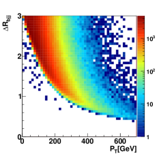
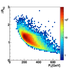
Figure 2: Left: partonic $\Delta R_{bjj}$ vs $p_{T}$ distribution for a Standard Model $t\bar{t}$ sample. Right: the same correlation, but only for tagged top quarks and based on the reconstructed kinematic properties.

Top taggers are algorithms identifying top quarks inside geometrically large and massive jets. They rely on the way a jet algorithm combines calorimeter towers into an actual jet. An obvious limitation is the geometrical size of the jet which for a successful tag has to include all three main decay products of the top quark. At the parton level we can compute the size of the top quark from the three $R$ distances of its main decay products: following the Cambridge/Aachen algorithm ca_algo ; fastjet we first identify the combination $(i,j)$ with the smallest $\Delta R_{ij}$. The length of the second axis in the top reconstruction we obtain from combining $i$ and $j$ and computing the $R$ distance of this vector to the third constituent. The maximum of the two $R$ distances gives the approximate partonic initial size $\Delta R_{bjj}$ of a C/A jet covering the main top decay products. In Figure 2 we first correlate this partonic top size with the transverse momentum of the top quark for a complete $t\bar{t}$ sample in the Standard Model. As expected, if for technical reasons we want to limit the size of the C/A fat jet to values below 1.5 we cannot expect to see top quarks with a partonic transverse momentum of $p_{T}\lesssim 150$ GeV. In the right panel we show the same correlation, but after tagging the top quark as described below and based on the reconstructed kinematics. The lower boundaries indeed trace each other, and the main body of tagged Standard Model top quarks resides in the $p_{T,t}^{\text{rec}}=200\cdots 250$ GeV range, correlated with $\Delta R_{bjj}^{\text{rec}}=1\cdots 1.5$. This result illustrates that for a Standard Model top tagger it is indeed crucial to start from a large initial jet size.

Therefore, our tagger for Standard Model tops is based on the Cambridge/Aachen ca_algo ; fastjet jet algorithm with $R=1.5$, combined with a mass-drop criterion fatjet_vh ; david_e ; fatjet_tth . Because the generic $p_{T}$ range for the tops does not exceed 500 GeV the granularity of the detector does not play a role, and we can optionally apply a $b$ tag to improve the QCD rejection rate. Since such a subjet $b$ tag giacinto will only enter as a probabilistic factor ($60\%,10\%,2\%$) for ($b,c,q/g$) jets we do not include it in the following discussion. Note that whenever we require a $b$ tag in our actual analysis, the numbers do not yet include the ($70\%,1\%$) improvements found for a $b$ tag inside a boosted Higgs giacinto .

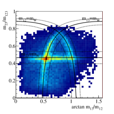
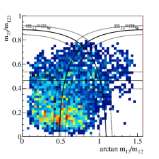
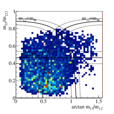
Figure 3: Distribution of all events in the $\arctan m_{13}/m_{12}$ vs $m_{23}/m_{123}$ plane. We show $t\bar{t}$ (left). $W$+jets (center) and pure QCD jets (right) samples. More densely populated regions of the phase space appear in red.

The algorithm proceeds in the following steps:

1. define a fat jet using the C/A algorithm with $R=1.5$

2. for each fat jet, find all hard subjets using a mass drop criterion: when undoing the last clustering of the jet $j$, into two subjets $j_{1},j_{2}$ with $m_{j_{1}}>m_{j_{2}}$, we require $m_{j_{1}}<0.8~{}m_{j}$ to keep $j_{1}$ and $j_{2}$. Otherwise, we keep only $j_{1}$. Each subjet $j_{i}$ we either further decompose (if $m_{j_{i}}>30~{}{\rm GeV}$) or add to the list of relevant substructures.

3. iterate through all pairings of three hard subjets: first, filter them with resolution $R_{\text{filter}}=\min(0.3,\Delta R_{jk}/2)$. Next, use the five hardest filtered constituents and calculate their jet mass (for less than five filtered constituents use all of them). Finally, select the set of three-subjet pairings with a jet mass closest to $m_{t}$.

4. construct exactly three subjets $j_{1},j_{2},j_{3}$ from the five filtered constituents, ordered by $p_{T}$. If the masses $(m_{12},m_{13},m_{23})$ satisfy one of the following three criteria, accept them as a top candidate:

   $$0.2<\arctan\frac{m_{13}}{m_{12}}<1.3\qquad\text{and}\quad R_{\min}<\frac{m_{23}}{m_{123}}<R_{\max}$$

   $$R_{\min}^{2}\left(1+\left(\frac{m_{13}}{m_{12}}\right)^{2}\right)<1-\left(\frac{m_{23}}{m_{123}}\right)^{2}<R_{\max}^{2}\left(1+\left(\frac{m_{13}}{m_{12}}\right)^{2}\right)\quad\text{and}\quad\frac{m_{23}}{m_{123}}>0.35$$

   $$R_{\min}^{2}\left(1+\left(\frac{m_{12}}{m_{13}}\right)^{2}\right)<1-\left(\frac{m_{23}}{m_{123}}\right)^{2}<R_{\max}^{2}\left(1+\left(\frac{m_{12}}{m_{13}}\right)^{2}\right)\quad\text{and}\quad\frac{m_{23}}{m_{123}}>0.35$$ (8)

   with $R_{\min}=85\%\times m_{W}/m_{t}$ and $R_{\max}=115\%\times m_{W}/m_{t}$. The numerical soft cutoff at 0.35 is independent of the masses involved and only removes QCD events. The distributions for top and QCD events we show in Fig. 3.

5. finally, require the combined $p_{T}$ of the three subjets to exceed 200 GeV.

In step 3 of the algorithm there exist many possible criteria to choose three jets from hard subjets inside a fat jet. For example, we can include angular information (the $W$ helicity angle) in the selection criterion and select the smallest $\Delta m_{t}+A_{W}\Delta m_{W}+A_{h}\Delta\cos_{h}$. In that case, the tagging efficiency increases, but simultaneously the fake rate also increases, so to reach the best signal significance we simply select the combination with the best $m_{t}$. This allows us to apply efficient orthogonal criteria based on the reconstructed $m_{W}$ and on the radiation pattern later.

In step 4, the choice of mass variables shown in Figure 3 is of course not unique. In general, we know that in addition to the two mass constraints ($m_{123}=m_{t}^{\text{rec}}$ as well as $m_{jk}=m_{W}^{\text{rec}}$ for one $(j,k)$) we can exploit one more mass or angular relation of the three main decay products. Our three subjets $j_{k}$ ignoring smearing and assuming $p_{i}^{2}\sim 0$ give

$$m_{t}^{2}\equiv m_{123}^{2}=(p_{1}+p_{2}+p_{3})^{2}=(p_{1}+p_{2})^{2}+(p_{1}+p_{3})^{2}+(p_{2}+p_{3})^{2}=m_{12}^{2}+m_{13}^{2}+m_{23}^{2}\;,$$ (9)

which is the surface of a sphere with radius $m_{t}$ in $(m_{12},m_{13},m_{23})$. For fixed $m_{123}$ we can pick exactly two more variables to fully describe the kinematics: we choose $m_{23}/m_{123}$ and $\arctan m_{13}/m_{12}$, which means that $m_{12}/m_{123}$ can be derived as

$$1=\left(\frac{m_{12}}{m_{123}}\right)^{2}\left(1+\left(\frac{m_{13}}{m_{12}}\right)^{2}\right)+\left(\frac{m_{23}}{m_{123}}\right)^{2}\;.$$ (10)

Assuming $m_{123}=m_{t}$ the condition $m_{12}=m_{W}\pm 15\%$ then reads $m_{12}/m_{123}=R_{\text{min}}\cdots R_{\text{max}}$, which is the form we use in Eq.(8). Note that our three mass conditions can also be written in terms of two masses and the $W$ helicity angle david_e ; fatjet_tth , but the construction of this angle requires a boost into the $W$ rest frame with its experimental challenges which we prefer to avoid. The switch from the helicity angle scheme to the pure mass scheme only has a negligible effect on the efficiencies computed without full detector simulation.

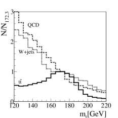
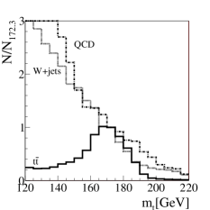
Figure 4: Number of tagged tops in the $t\bar{t}$, QCD jets and $W$+jets channels for a varying assumed top mass in the tagging algorithm. The actual top mass in the sample is 172.3 GeV. Shown is the number of tagged first (left) and second (right) tops.

Finally, in contrast to the Higgs tagger fatjet_vh ; fatjet_tth the top tagger does know about the top mass when searching for the two mass drops. This means that we will not be able to apply a side-bin normalization. However, we can access side bins by changing the assumed $m_{t}$ as used in the algorithm, Eq.(8), to values different from the top mass in the event sample. The result of such a misalignment we show in Figure 4: for the QCD and $W$+jets background the number of tagged tops follows the typical $p_{T}$ dependence of the jet sample. The lower the top mass we are looking for the more tagged tops we will find. In contrast, the top sample shows a clear peak when the assumed top mass in the algorithm coincides with the top mass in the sample. Towards larger assumed top masses the distribution shows a one-sided width around 20 GeV. Towards smaller assumed top masses additional QCD jets can have an increasing impact on wrongly tagged tops. Therefore, the tail is considerably higher. While this kind of behavior makes it unlikely that such side-bins will useful for an actual analysis they serve as a very useful cross check for our fat-jet methods.

In Figure 5 we summarize the performance of the tagging algorithm described above. In the left panel, we show the parton-level $p_{T}$ of the hadronic top quarks in the $t\bar{t}$ sample, normalized to the top production rate. As we already know from Figure 2 this distribution drops rapidly and essentially vanishes for $p_{T}>500$ GeV. This is the reason why our tagging algorithm focuses on a top $p_{T}$ range between 200 and 500 GeV. The curve for tagged tops follows the curve for produced tops smoothly for $p_{T}>250$ GeV. The same curve for tagged tops is actually included in all three panels, different just because of the normalization of the plots. The two curves for mis-tagged tops in the $W$+jets and QCD sample are shown as a function of the reconstructed $p_{T}$ of the top constituents in the last step of our algorithm. Again, they are normalized to the production rate at the LHC, so we immediately see that one top tag will not be sufficient to reduce the pure QCD background to the level of top pair production. The $W$+jets background, in contrast, should not pose a problem to fat-jet analyses, which we confirm in our actual analysis and show in Table 2.

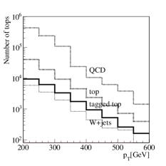
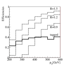
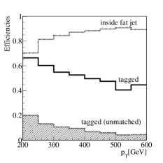
Figure 5: Left: number of tops, tagged tops, mis-tagged tops from QCD jets and for $W$+jets for $1~{}{\rm fb^{-1}}$. Center: fraction of hadronic tops whose main parton-level decay products are within a C/A distance of $\Delta R_{bjj}=1.5,1.2,0.9$. Right: tagging efficiencies, normalized to the top line of the central panel.

In the center panel of Figure 5 we show the fraction of tops found inside C/A distances of $\Delta R_{bjj}<0.9,1.2,1.5$, normalized to the number of tops produced (i.e.  the top production line in the left panel). As indicated in Figure 2, in particular in the promising Standard Model range $p_{T,t}<300$ GeV we lose the vast majority of events if we reduce the jet size from $R=1.5$ to $R=1.2$. We also show the fraction of tagged tops based on $R=1.5$, showing an efficiency of 20% to 40% relative to all tops produced.

In the right panel of Figure 5 we show the top tagging efficiency as a function of the reconstructed top $p_{T}$, normalized to the number of tops within $\Delta R_{bjj}<1.5$ (the top line in the center panel). The first line shows how many of the tops end up with all main parton-level decay products inside the fat jet, as requested in step 1 of our algorithm. There is a loss associated with this actual construction of the fat jet, because even if all main top decay products are close enough to end up inside a fat jet of size $R=1.5$, they do not have to. For example, the geometric center of the fat jet can be slightly shifted, so one of the top decay products drops out. The second line shows the fraction of tagged tops. The shading indicates the fraction of these tops where we cannot establish a one-to-one connection between the three subjets constructed in step 4 and the parton-level top decay products.

To establish such a connection we compute the $R$ distances between the three subjets and all hard partons in the event. We then identify the parton pairing which gives the smallest value of $\Delta R_{ijk}^{2}=\Delta R(j_{1},p_{i})^{2}+\Delta R(j_{2},p_{j})^{2}+\Delta R(j_{3},p_{k})^{2}$ and check if this pairing corresponds to a top decay at parton level. If not, we assume that either a QCD jet might have entered the reconstruction or that QCD radiation has bent one of the top decay jets far away from its partonic origin. However, this rate is considerably higher than the $W$+jets mis-tag rate, so these events are not dominated by continuum QCD jet production. Instead, they represent the generic problem of identifying partons with jets by some kind of geometric measure. In a way these tags are the tricky ones for low transverse momenta, while the efficiency for identifiable tags is a fairly constant $\mathcal{O}(40\%)$ over the entire $p_{T}$ range.

	$t\bar{t}$			QCD	$W$+jets	$t\bar{t}$			QCD	$W$+jets
$p_{T,t}^{\text{min}}[{\rm GeV}]$	0	200	300			0	200	300
one fat jet	$92200$	$36100$	$8250$	$4.10\cdot 10^{7}$	$3.19\cdot 10^{5}$	100%	100%	100%	100%	100%
two fat jets	$40700$	$20300$	$5810$	$2.16\cdot 10^{7}$	$1.60\cdot 10^{5}$	44%	57%	70%	53%	50%	relative to one fat jet
one top tag	$20900$	$13400$	$4160$	$8.18\cdot 10^{5}$	$1.27\cdot 10^{4}$	23%	37%	51%	2.0%	3.9%	relative to one fat jet
two top tags	$1880$	$1630$	$700$	$11000$	$233$	2.0%	4.5%	8.5%	0.027%	0.07%	relative to one fat jet
						4.5%	8.0%	12%	0.05%	0.15%	relative to two fat jets

Table 3: Number of events in $1~{}{\rm fb^{-1}}$ and their relative tagging efficiencies for the first and the second top tag in the different Standard Model event samples. One top tag and one fat jet means at least one tag or fat jet. Fat jets are defined with $p_{T}>200$ GeV. The top quarks are produced with $p_{T}>0,200,300$ GeV at parton level. All rates are quoted at leading order.

The bottom line in terms of tagging efficiencies and mis-tagging probabilities we show in Table 3: provided we find something like a fat jet a top can be tagged with an efficiency of 23% to 51%, dependent on the $p_{T}$ range of the top. This variation shows that for low generated $p_{T,t}$ there will still be a fat jet in the $t\bar{t}$ sample, but this fat jet will tend to not include the top decay products, so we cannot tag a top to begin with.

For a second top tag we first need to see another fat jet in the sample. For top pairs this will happen in 44% of all events, up to 70% for hard tops. However, there are two tops in the event, and there will likely be two fat jets. For $p_{T,t}>200$ GeV the 37% tagging efficiency quoted in Table 3 corresponds to a 26% efficiency of tagging a top in a given fat jet. Based on this number we can compute the probability of tagging two tops in two fat jets, which gives slightly less than 4%. So in particular for low-$p_{T}$ tops our efficiency for a second top tag is higher than for the first. For the signal discussed in the main body of the paper we would need to fold this efficiency with the $p_{T}$ spectrum of tops from stop decays. From the 200 GeV and 300 GeV columns in Table 3 we see that this will help considerably.

For $W$+jets and pure QCD jets with their generically softer QCD structure it will not be as likely to actually find the first fat jet in the sample. In addition, the mis-tagging rate for the first top tag after seeing a fat jet ranges around 2% to 4%. The efficiency for a second fat jet in the background processes is almost as large as for top pairs. This reflects the fact that one hard fat jet has to recoil against QCD activity which will give us a second fat jet. The probability of mis-tagging two tops is then roughly the first mis-tag probability squared, after factoring out the probabilities of finding one or two fat jets. This way, the over-all efficiencies for two top tags significantly enhance the signal-to-background ratio, in particular for pure QCD jets. As mentioned several times, this number can be improved if we ask for a $b$ tag inside the top jet. As a last comment, our top tagger is optimized for low $p_{T,t}$, so further work and modifications should be able to increase its efficiency towards higher boosts.

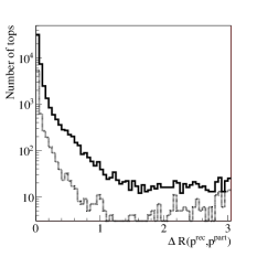
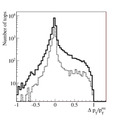
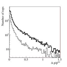
Figure 6: From left to right: $\Delta R$ between the reconstructed and the parton-level top quark; $\Delta p_{T}/p_{T}^{\text{rec}}$ for the same sample; $\Delta p/p^{\text{rec}}$ where $p$ denotes the absolute value of the top 3-momentum. The solid curves correspond to the default $p_{T,t}^{\text{rec}}>200$ GeV of the tagged top, while the dashed curves constrains the tagged top to values above $p_{T,t}^{\text{rec}}>300$ GeV.

The last question beyond the simple top tag is how well the algorithm described in this Appendix can reconstruct the top momentum. In principle, our top tagging algorithm can identify the three subjets as either $W$-decay jets or the $b$ jet. Unfortunately, even amongst the events which allow for a clear comparison of the partonic top decay products and the resulting subjets a fair fraction returns $m_{bj}\sim 80$ GeV on the parton level. This is because the invariant masses of all jet combinations reside in the same range, out of which our $W$ mass window represents a sizeable fraction. To test for such effects we can take all tagged tops in the hadronic $t\bar{t}$ sample and compare the reconstructed top momenta to the parton-level input. In Figure 6 we first show the angular distance of the reconstructed top quarks from the parton-level truth.

While there is a strong peak for $\Delta R<0.5$ and 95% of the events resides in the area, we also observe a long tail at the $10^{-3}$ level, which is due to combinatorics or effective QCD mis-tags in the top sample. In the second panel we show the relative error on the transverse momentum of the tagged top ($\Delta p_{T}=p_{T}^{\text{rec}}-p_{T}^{\text{part}}$). For around 85% of the events the mis-measurement compared to the parton-level truth stays below the 20% level. In the third panel we show the same for the entire 3-momentum. Again, 68% of the tops are reconstructed at the 10% level, while 80% are reconstructed within $\Delta p/p\sim 20\%$. Obviously, all these numbers can be improved if we increase the $p_{T}^{\text{min}}$ cut on the reconstructed top for example from 200 GeV to 300 GeV.

References

- (1) D. E. Morrissey, T. Plehn and T. M. P. Tait, arXiv:0912.3259 [hep-ph].
- (2) P. Meade and M. Reece, Phys. Rev. D 74, 015010 (2006).
- (3) A. Djouadi, W. Hollik and C. Jünger, Phys. Rev. D 54, 5629 (1996); S. Kraml, H. Eberl, A. Bartl, W. Majerotto and W. Porod, Phys. Lett. B 386, 175 (1996); W. Beenakker, R. Höpker, T. Plehn and P. M. Zerwas, Z. Phys. C 75, 349 (1997).
- (4) T. Aaltonen et al. [CDF Collaboration], CDF Note 9834, 2009; V. M. Abazov et al. [D0 Collaboration], Phys. Lett. B 665, 1 (2008).
- (5) T. Aaltonen et al. [CDF Collaboration], arXiv:0912.1308 [hep-ex]; V. M. Abazov et al. [D0 Collaboration], Phys. Lett. B 675, 289 (2009).
- (6) G. L. Bayatian et al. [CMS Collaboration], J. Phys. G 34, 995 (2007).
- (7) P. Langacker, G. Paz, L. T. Wang and I. Yavin, JHEP 0707, 055 (2007); J. Ellis, F. Moortgat, G. Moortgat-Pick, J. M. Smillie and J. Tattersall, Eur. Phys. J. C 60, 633 (2009); K. Rolbiecki, J. Tattersall and G. Moortgat-Pick, arXiv:0909.3196 [hep-ph]; M. Blanke, D. Curtin and M. Perelstein, arXiv:1004.5350 [hep-ph].
- (8) M. Perelstein and A. Weiler, JHEP 0903, 141 (2009).
- (9) J. M. Butterworth, A. R. Davison, M. Rubin and G. P. Salam, Phys. Rev. Lett. 100, 242001 (2008); D. E. Soper and M. Spannowsky, arXiv:1005.0417 [hep-ph].
- (10) D. E. Kaplan, K. Rehermann, M. D. Schwartz and B. Tweedie, Phys. Rev. Lett. 101, 142001 (2008).
- (11) T. Plehn, G. P. Salam and M. Spannowsky, Phys. Rev. Lett. 104, 111801 (2010).
- (12) W. Beenakker, M. Krämer, T. Plehn, M. Spira and P. M. Zerwas, Nucl. Phys. B 515, 3 (1998).
- (13) P. Nason, S. Dawson and R. K. Ellis, Nucl. Phys. B 303, 607 (1988); W. Beenakker, H. Kuijf, W. L. van Neerven and J. Smith, Phys. Rev. D 40, 54 (1989); S. Moch and P. Uwer, Phys. Rev. D 78, 034003 (2008).
- (14) see e.g. V. Barger, T. Han and D. G. E. Walker, Phys. Rev. Lett. 100, 031801 (2008); U. Baur and L. H. Orr, Phys. Rev. D 76, 094012 (2007); T. Han, R. Mahbubani, D. G. E. Walker and L. T. E. Wang, JHEP 0905, 117 (2009).
- (15) G. Corcella et al., arXiv:hep-ph/0210213; M. Bahr et al , arXiv:0812.0529 [hep-ph].
- (16) T. Sjostrand, S. Mrenna and P. Z. Skands, JHEP 0605, 026 (2006); T. Sjostrand, S. Mrenna and P. Z. Skands, Comput. Phys. Commun. 178, 852 (2008).
- (17) M. L. Mangano, M. Moretti, F. Piccinini, R. Pittau and A. D. Polosa, JHEP 0307, 001 (2003).
- (18) E. Richter-Was, arXiv:hep-ph/0207355.
- (19) G. Aad et al. [The ATLAS Collaboration], arXiv:0901.0512 [hep-ex].
- (20) for a similar conclusion see e.g. A. Freitas and D. Wyler, JHEP 0611, 061 (2006).
- (21) M. H. Seymour, Z. Phys. C 62, 127 (1994); J. M. Butterworth, B. E. Cox and J. R. Forshaw, Phys. Rev. D 65, 096014 (2002); W. Skiba and D. Tucker-Smith, Phys. Rev. D 75, 115010 (2007); B. Holdom, JHEP 0703, 063 (2007).
- (22) J. M. Butterworth, J. R. Ellis and A. R. Raklev, JHEP 0705, 033 (2007); J. M. Butterworth, J. R. Ellis, A. R. Raklev and G. P. Salam, arXiv:0906.0728 [hep-ph]; C. S. Cowden, S. T. French, J. A. Frost and C. G. Lester [The ATLAS Collaboration], ATLAS-PHYS-PUB-2009-076, June 2009; G. D. Kribs, A. Martin, T. S. Roy and M. Spannowsky, arXiv:0912.4731 [hep-ph] and arXiv:1006.1656 [hep-ph].
- (23) C. R. Chen, M. M. Nojiri and W. Sreethawong, arXiv:1006.1151 [hep-ph]; A. Falkowski, D. Krohn, J. Shelton, A. Thalapillil and L. T. Wang, arXiv:1006.1650 [hep-ph].
- (24) Y. L. Dokshitzer, G. D. Leder, S. Moretti and B. R. Webber, JHEP 9708, 001 (1997); M. Wobisch and T. Wengler, arXiv:hep-ph/9907280.
- (25) M. Cacciari and G. P. Salam, Phys. Lett. B 641, 57 (2006); M. Cacciari, G. P. Salam and G. Soyez, http://fastjet.fr
- (26) C. G. Lester and D. J. Summers, Phys. Lett. B 463, 99 (1999); A. Barr, C. Lester and P. Stephens, J. Phys. G 29, 2343 (2003).
- (27) see e.g. U. Baur and L. H. Orr, Phys. Rev. D 77, 114001 (2008); P. Fileviez Perez, R. Gavin, T. McElmurry and F. Petriello, Phys. Rev. D 78, 115017 (2008); Y. Bai and Z. Han, JHEP 0904, 056 (2009).
- (28) K. Agashe, A. Belyaev, T. Krupovnickas, G. Perez and J. Virzi, Phys. Rev. D 77, 015003 (2008); M. Gerbush, T. J. Khoo, D. J. Phalen, A. Pierce and D. Tucker-Smith, Phys. Rev. D 77, 095003 (2008); G. Brooijmans, ATL-PHYS-CONF-2008-008 and ATL-COM-PHYS-2008-001, Feb. 2008 J. Thaler and L. T. Wang, JHEP 0807, 092 (2008); L. G. Almeida, S. J. Lee, G. Perez, G. Sterman, I. Sung and J. Virzi, Phys. Rev. D 79, 074017 (2009); L. G. Almeida, S. J. Lee, G. Perez, I. Sung and J. Virzi, Phys. Rev. D 79, 074012 (2009); D. Krohn, J. Thaler and L. T. Wang, arXiv:0903.0392 [hep-ph].
- (29) S. D. Ellis, C. K. Vermilion and J. R. Walsh, arXiv:0903.5081 [hep-ph] and arXiv:0912.0033 [hep-ph].
- (30) ATLAS note, ATL-PHYS-PUB-2009-088.
- (31) J. Hisano, K. Kawagoe and M. M. Nojiri, Phys. Rev. D 68, 035007 (2003); G. Weiglein et al. [LHC/LC Study Group], Phys. Rept. 426, 47 (2006).
- (32) R. Lafaye, T. Plehn, M. Rauch and D. Zerwas, Eur. Phys. J. C 54, 617 (2008); P. Bechtle, K. Desch, M. Uhlenbrock and P. Wienemann, [arXiv:0907.2589 [hep-ph]].