Probing top flavour-changing neutral scalar couplings at the CERN LHC

Abstract

Top decays into a light Higgs boson and an up or charm quark can reach detectable levels in Standard Model extensions with two Higgs doublets or with new exotic quarks, and in the Minimal Supersymmetric Standard Model. Using both a standard and a neural network analysis we show that the CERN Large Hadron Collider will give $3\,\sigma$ evidence of decays with $\mathrm{Br}(t\to Hc)\geq 6.5\times 10^{-5}$ or set a limit $\mathrm{Br}(t\to Hc)\leq 4.5\times 10^{-5}$ with a 95% confidence level if these decays are not observed. We also consider limits obtained from single top production associated with a neutral Higgs boson.

PACS: 12.15.Mm; 12.60.Fr; 14.65.Ha; 14.80.Cp

UG–FT–113/00
                                                                                                            FIST/4-2000/CFIF
                                                                                                            hep-ph/0004190
                                                                                                            April 2000

1 Introduction

The search for flavour-changing neutral (FCN) current processes both at high and low energies is one of the major tools to test the Standard Model (SM), with the potential for either discovering or putting stringent limits on new physics. In the SM, there are no gauge FCN couplings at tree level due to the GIM mechanism, and scalar couplings are also automatically flavour-diagonal provided only one Higgs doublet is introduced. However, there is no fundamental reason for having only one Higgs doublet, and for two or more scalar doublets FCN couplings are generated at tree level unless an ad hoc discrete symmetry is imposed [1].

There are stringent limits on the FCN couplings between light quarks arising from the smallness of the $K^{0}-\bar{K}^{0}$, $B^{0}-\bar{B}^{0}$ and $D^{0}-\bar{D}^{0}$ mass differences [2], as well as from the CP violation parameter $\epsilon$ of the neutral kaon system. If there is no suppression of scalar FCN couplings, the masses of the neutral Higgs bosons have to be of the order of 1 TeV. However, if FCN couplings between light quarks are suppressed, being for instance proportional to the quark masses [3, 4] or to some combination of Cabibbo-Kobayashi-Maskawa (CKM) mixing angles [5, 6], the lightest neutral Higgs may have a mass $M_{H}$ of around 100 GeV. In this case, the effects of scalar FCN currents involving the top quark can be quite sizeable.

The interactions among the top, a light quark $q=u,c$ and a Higgs boson $H$ will be described by the effective Lagrangian

$$\mathcal{L}=\frac{g_{W}}{2\sqrt{2}}g_{tq}\bar{q}(c_{v}+c_{a}\gamma_{5})tH~{}~{}+~{}\mathrm{h.c.}$$ (1)

The axial and vector parts of the coupling are normalized to $|c_{v}|^{2}+|c_{a}|^{2}=1$. The natural size of $g_{tc}$ in a two Higgs doublet model (2HDM) is $g_{tc}\sim 0.20$, leading to large FCN current effects observable at the CERN Large Hadron Collider (LHC). The natural size of $g_{tu}$ ranges from 0.012 to 0.025, depending on the model considered. This is too small to be observed, but if this coupling is enhanced by a factor $\sim 2$, it could also be detected. Models with new heavy exotic quarks can also have large tree level $Htq$ couplings, with the particularity that they are proportional to the FCN $Ztq$ couplings [7]. Present limits on the latter [8] allow for $g_{tu}\sim 0.31$ or $g_{tc}\sim 0.35$, both observable at LHC.

The large top quark mass opens the possibility of having relatively large effective vertices $Htq$ induced at one loop by new physics. In the Minimal Supersymmetric Standard Model (MSSM) there are large regions of the parameter space where one can have $g_{tc}\sim 0.04$ [9, 10] . In contrast, in the SM the effective $Htc$ vertex is very small, $g_{tc}\sim 10^{-6}$ due to a strong GIM cancellation [11]. The large top quark mass also suggests that the top quark could play a fundamental rôle in the electroweak symmetry breaking mechanism [12, 13] and in this case top FCN scalar couplings would be large, $g_{tc}\sim 0.3-0.4$ [14] or $g_{tc}\sim 0.5-2.9$ [15], depending on the model considered. Hence the importance of measuring its couplings, in particular to the Higgs boson [16].

Present experimental bounds on top FCN scalar (and gauge) couplings are very weak. Some processes have been proposed to measure the $Htq$ vertices, for instance $t\bar{c}\nu_{e}\bar{\nu}_{e}$ and $t\bar{c}e^{+}e^{-}$ production at a linear collider with a center of mass (CM) energy of $1-2$ TeV [17] and $t\bar{c}$ production at a muon collider [18] or at hadron colliders via gluon fusion $gg\to H\to t\bar{c}$ [14]. These processes can probe the FCN couplings of the heavier mass eigenstates, but do not provide useful limits for the light scalars. In this Letter we will show that top decays $t\to Hq$ at LHC provide the best limits on the couplings of a light scalar of a mass slightly above 100 GeV. The importance of this mass range stems from the fact that global fits to electroweak observables in the SM [19] seem to prefer $M_{H}\sim 100$ GeV, as well as the MSSM prediction that the mass of the lightest scalar has to be less than 130 GeV [20]. On the other hand, direct searches at the CERN $e^{+}e^{-}$ collider LEP at CM energies up to 202 GeV imply the bound $M_{H}>107.9$ GeV for the mass of a SM Higgs, with a 95% confidence level (CL) [21]. For the lightest Higgs of the MSSM the bounds depend on the choice of parameters and typically are reduced to $M_{H}>88.3$ GeV.

In the following we will perform a detailed analysis of the sensitivity of the LHC to FCN scalar couplings in top decays $t\to Hq$ [22]. We will also study $Ht$ production, which also serves to constrain the $Htq$ vertex [23]. However, the bounds obtained from this process are much less restrictive. Finally, we will comment on the potential of the LHC to discover these signals at the rates predicted by some models.

2 Limits on FCN couplings from top decays

To obtain constraints on the coupling $g_{tq}$ we will first consider $t\bar{t}$ production, with the top quark decaying to $W^{+}b\to l\nu b$, $l=e,\mu$ and the antitop decaying to $H\bar{q}$. With a good $\tau$ identification the decays $W^{+}\to\tau^{+}\nu$ can be included, improving the statistical significance of the signal.

The decay mode of the Higgs boson depends strongly on its mass. For our evaluation, we take $M_{H}=120$ GeV, well above the LEP limits, and decaying into $b\bar{b}$ pairs. In principle, there is no reason to assume that the $Hbb$ coupling is suppressed. In a general 2HDM, both doublets couple to the $b$ quark and, unless some fine-tuned cancellation occurs, the coupling of the physical light Higgs to the $b$ quark is proportional to the $b$ mass, which we take $m_{b}=3.1$ GeV at the scale $\mu=M_{H}$. To be conservative, we assume that the Higgs couplings to the gauge bosons are not suppressed and are the same as in the SM. Thus for $M_{H}=120$ GeV $H$ decays predominantly into $b\bar{b}$ pairs, with a branching ratio of $0.7$. For $M_{H}>130$ GeV, the $W^{+}W^{-}$ decay mode, with one of the $W$’s off-shell, begins to dominate . The signal is then $l\nu bb\bar{b}j$, with three $b$ quarks in the final state. Clearly, $b$ tagging is crucial to separate the signal from the backgrounds. We assume a $b$ tagging efficiency of 50%, and a mistag rate of 1%, similar to the values recently achieved at SLD [24].

We evaluate the signal using the full $gg,q\bar{q}\to t\bar{t}\to W^{+}bH\bar{q}\to l\nu bb\bar{b}q$ matrix elements with all intermediate particles off-shell. We calculate the matrix elements using HELAS [25] code generated by MadGraph [26] and modified to include the decay chain. For definiteness we assume $c_{v}=1$, $c_{a}=0$, but we check that the difference when using other combinations is below $1\%$. We normalize the cross section with a $K$ factor of 2.0 [27].

The main background to this signal comes from $t\bar{t}$ production with standard top and antitop decays, $t\to W^{+}b\to l\nu b$, $\bar{t}\to W^{-}\bar{b}\to jj\bar{b}$. This process mimics the signal if one of the jets resulting from the $W^{-}$ decay is mistagged as a $b$ jet. The matrix elements for this process are calculated with HELAS and MadGraph in the same way as the signal, taking again $K=2.0$. Another background to be considered is $Wb\bar{b}jj$ production, for which we use VECBOS [28] modified to include energy smearing and trigger and kinematical cuts. For this process we take $K=1.1$ [29]. $Wjjjj$ production is negligible after using $b$ tagging. For the phase space integration we use MRST structure functions set A [30] with $Q^{2}=\hat{s}$.

After generating signals and backgrounds, we simulate the detector resolution effects with a Gaussian smearing of the energies of jets $j$ and charged leptons $l$ [31],

$$\frac{\Delta E^{l}}{E^{l}}=\frac{10\%}{\sqrt{E^{l}}}\oplus 0.3\%\,,~{}~{}~{}~{}\frac{\Delta E^{j}}{E^{j}}=\frac{50\%}{\sqrt{E^{j}}}\oplus 3\%\,,$$ (2)

where the energies are in GeV and the two terms are added in quadrature. We then apply detector cuts on transverse momenta $p_{T}$, pseudorapidities $\eta$ and distances in $(\eta,\phi)$ space $\Delta R$:

$$p_{T}^{l}\geq 15~{}\mathrm{GeV}~{},~{}~{}p_{T}^{j}\geq 20~{}\mathrm{GeV}$$

$$|\eta^{l,j}|\leq 2.5~{},~{}~{}\Delta R_{jj,lj}\geq 0.4\,.$$ (3)

For the events to be triggered, we require both the signal and background to fulfill at least one of the trigger conditions [32]. These conditions are different in the low 10 fb^-1 (L) and high 100 fb^-1 (H) luminosity Runs. For our processes, the relevant conditions are

• one jet with $p_{T}\geq 180$ GeV (L) / 290 GeV (H),

• three jets with $p_{T}\geq 75$ GeV (L) / 130 GeV (H),

• one charged lepton with $p_{T}\geq 20$ GeV (L) / 30 GeV (H),

• missing energy $E_{T}\!\!\!\!\!\!\!\!\!\not\,\,\,\,\,\,\,\geq 50$ GeV (L) / 100 GeV (H) and one jet with $p_{T}\geq 50$ GeV (L) / 100 GeV (H).

We reconstruct the signal as follows. There are three tagged $b$ jets $b_{1-3}$ in the final state and a non-$b$ jet $j$. There are three possible pairs $b_{i},b_{j}$, with invariant masses $M_{b_{i}b_{j}}$, one of which results from the decay of the Higgs boson and has an invariant mass close to $M_{H}$. The invariant mass of this pair and the jet $j$, $M_{b_{i}b_{j}j}$, is also close to the top mass. Hence we choose the pair $b_{i},b_{j}$ which minimizes $(M_{b_{i}b_{j}}-M_{H})+(M_{b_{i}b_{j}j}-m_{t})$, defining the Higgs reconstructed mass as $M_{H}^{\mathrm{rec}}=M_{b_{i}b_{j}}$ and the antitop reconstructed mass as $m_{\bar{t}}^{\mathrm{rec}}=M_{b_{i}b_{j}j}$. In Figs 1, 2 we plot the kinematical distributions of these variables for the signal and for the $t\bar{t}$ background. The $m_{\bar{t}}^{\mathrm{rec}}$ distribution is slightly broader for $t\bar{t}$ due to the signal reconstruction method.

Figure 1: Reconstructed Higgs mass $M_{H}^{\mathrm{rec}}$ distribution before kinematical cuts for the signal and $t\bar{t}$ background in LHC Run L. We use $g_{tq}=0.2$.

Figure 2: Reconstructed antitop mass $m_{\bar{t}}^{\mathrm{rec}}$ distribution before kinematical cuts for the signal and $t\bar{t}$ background in LHC Run L. We use $g_{tq}=0.2$.

The remaining jet $b_{k}$ and the charged lepton result from the decay of the top quark. To reconstruct its mass, we make the hypothesis that all missing energy comes from a single neutrino with $p^{\nu}=(E^{\nu},p_{T}\!\!\!\!\!\!\!\!\not\,\,\,\,\,\,\,,p_{L}^{\nu})$, and $p_{T}\!\!\!\!\!\!\!\!\not\,\,\,\,\,\,\,$ the missing transverse momentum. Using $(p^{l}+p^{\nu})^{2}=M_{W}^{2}$ we find two solutions for $p^{\nu}$, and we choose that one making the reconstructed top mass $m_{t}^{\mathrm{rec}}\equiv\sqrt{(p^{l}+p^{\nu}+p^{b_{k}})^{2}}$ closest to $m_{t}$. In Fig. 3 we plot the kinematical distribution of this variable for the signal and $t\bar{t}$ background.

Figure 3: Reconstructed top mass $m_{t}^{\mathrm{rec}}$ distribution before kinematical cuts for the signal and $t\bar{t}$ background in LHC Run L. We use $g_{tq}=0.2$.

The reconstruction of the signal and the requirement $m_{t}^{\mathrm{rec}},m_{\bar{t}}^{\mathrm{rec}}\sim m_{t}$, $M_{H}^{\mathrm{rec}}\sim M_{H}$ are sufficient to eliminate the $Wb\bar{b}jj$ background, but hardly affect $t\bar{t}$, as can be seen in Figs. 1–3. To improve the signal to background ratio we reject events when one pair of jets, $b_{i}j$ or $b_{j}j$, seems to be the product of the hadronic decay of a $W$ boson, as happens for the $t\bar{t}$ background. We define the reconstructed $W$ mass as the invariant mass $M_{b_{i}j}$, $M_{b_{j}j}$ closest to $M_{W}$ (see Fig. 4) and impose a veto cut on events with $M_{W}^{\mathrm{rec}}\sim M_{W}$.

Figure 4: Reconstructed $W$ mass $M_{W}^{\mathrm{rec}}$ distribution before kinematical cuts for the signal and $t\bar{t}$ background in LHC Run L. We use $g_{tq}=0.2$.

The complete set of kinematical cuts for both Runs is summarized in Table 1. We also require a large transverse energy $H_{T}$.

Variable	Cut
$M_{H}^{\mathrm{rec}}$	110–130
$m_{\bar{t}}^{\mathrm{rec}}$	160–185
$m_{t}^{\mathrm{rec}}$	160–190
$M_{W}^{\mathrm{rec}}$	$<65$ or $>110$
$H_{T}$	$>240$

Table 1: Standard kinematical cuts for the $l\nu bb\bar{b}j$ signal. The masses and the energy are in GeV.

Alternatively, we can use an artificial neural network (ANN) as a classifier to distinguish between the signal and the $t\bar{t}$ background. In addition to $M_{H}^{\mathrm{rec}}$, $m_{\bar{t}}^{\mathrm{rec}}$, $m_{t}^{\mathrm{rec}}$ and $M_{W}^{\mathrm{rec}}$, we consider $p_{T}^{H}$, the transverse momentum of the reconstructed Higgs boson, $p_{T}^{\mathrm{max}}$ and $p_{T}^{\mathrm{min}}$, the maximum and minimum transverse momentum of the jets, and $p_{T}^{b,\mathrm{max}}$, the maximum transverse momentum of the two $b$’s which reconstruct the Higgs boson. The kinematical distributions of these variables are shown in Figs. 5–8.

Figure 5: Higgs transverse momentum $p_{T}^{H}$ distribution before kinematical cuts for the signal and $t\bar{t}$ background in LHC Run L. We use $g_{tq}=0.2$.

Figure 6: $p_{T}^{\mathrm{max}}$ distribution before kinematical cuts for the signal and $t\bar{t}$ background in LHC Run L. We use $g_{tq}=0.2$.

Figure 7: $p_{T}^{\mathrm{min}}$ distribution before kinematical cuts for the signal and $t\bar{t}$ background in LHC Run L. We use $g_{tq}=0.2$.

Figure 8: $p_{T}^{b,\mathrm{max}}$ distribution before kinematical cuts for the signal and $t\bar{t}$ background in LHC Run L. We use $g_{tq}=0.2$.

We observe that these variables are clearly not suitable to perform kinematical cuts on them. However, their inclusion as inputs to an ANN greatly improves its ability to classify signal and background events. We have not found any improvement adding other variables, and in some cases the results are worse.

To construct the ANN we use JETNET 3.5 [33]. We find convenient using a three-layer topology of 8 input nodes, 12 hidden nodes and 1 output node. However, we do not claim that either the choice of variables or the network topology are the best ones. The performance of the ANN is not very sensitive to the number of hidden nodes. The input variables are normalized to lie approximately in the interval $[-1,1]$ to reduce the training time. The network output $r$ is set to one for the signal and zero for $t\bar{t}$. We train the network using two sets with roughly 40000 signal and 40000 background events and the standard backpropagation algorithm. To test the ability of the network to classify never seen data we use two other sets with the same size.

One frequent problem is overtraining. To avoid it, we keep training while the network error evaluated on the test sets, $E_{t}^{(N)}$, decreases for the successive training epochs $N$. When it begins to increase, we stop training. To avoid fluctuations, we keep track of $E_{t}^{(N)}$ for previous epochs. When we reach an epoch $N_{0}$ when $E_{t}^{(N_{0}-100)}$ is smaller than all the following values, we stop training and start again until epoch $N_{0}-100$.

We repeat the same procedure using four other different training and test sets of the same size, and find that the results are fairly stable. The final training is done including the 4 training and 4 test sets. At the end of the training, most of the signal and background events in the test samples concentrate in very narrow intervals $[0.99,1]$ and $[0,0.01]$, respectively.

To classify signal and background we use two other signal and background sets with never seen before data, 50 and 100 times larger, respectively, than the ones used in training, to avoid possible statistical fluctuations. To separate signal from background we simply require $r>0.998$. This maintains 29% of the signal while it rejects 99.9% of the $t\bar{t}$ background. It is not necessary to train another ANN to distinguish the $Wb\bar{b}jj$ background, the same network with $r>0.998$ completely eliminates it. In Table 2 we collect the number of events without cuts, with the standard cuts in Table 1 and with the ANN cut $r>0.998$, for LHC Runs L and H. We normalize the signal to $g_{tq}=0.2$.

	Run L			Run H
	before	standard	ANN	before	standard	ANN
	cuts	cuts	cuts	cut	cuts	cut
Signal	267	98.2	76.2	2150	797	614
$t\bar{t}$	7186	33.2	10.0	58230	270	80
$Wb\bar{b}jj$	77	0.3	0.1	644	2.2	1.0

Table 2: Number of $l\nu bb\bar{b}j$ events before and after kinematical cuts for the signal and backgrounds. We use $g_{tq}=0.2$.

Although for definiteness we train the ANN with a vector FCN coupling ($c_{v}=1$, $c_{a}=0$), we check that the same ANN correctly recognizes the signal events when we consider an axial, left- or right-handed FCN coupling. The differences between the cross sections are in all cases below $1\%$, and comparable to the statistical Monte Carlo uncertainty. The differences between the cross sections after standard kinematical cuts are also smaller than $1\%$.

To derive upper bounds on the FCN couplings we follow the Feldman-Cousins construction [34]. For the numerical evaluation of the confidence intervals we use the PCI package [35]. If there is no evidence of this process, i. e., if the number of events observed $n_{0}$ is equal to the expected background $n_{b}$, we obtain independent limits on the couplings $g_{tu}$, $g_{tc}$. Using the standard cuts we obtain $g_{tq}\leq 0.071$ at Run L and $g_{tq}\leq 0.041$ at Run H. Using the ANN cut improves these limits, $g_{tq}\leq 0.064$ at Run L and $g_{tq}\leq 0.035$ at Run H. All bounds are calculated with a 95% CL. Although the improvement may not seem very significant, in Section 4 we will see that the luminosity required to see a positive signal is reduced to one half with the help of the neural network.

It is worth to give here also the results for the Fermilab Tevatron. This process at Run II with a CM energy of 2 TeV and a luminosity of 20 fb^-1 gives only $g_{tq}\leq 0.38$ (using standard kinematical cuts) due to the smaller statistics available.

3 Limits on FCN couplings from $Ht$ production

The existence of top FCN Higgs couplings leads to $Ht$ production through the diagrams in Fig. 9. This process has a negligible cross section in the SM [36]. As in the previous section, we consider only the leptonic decays of the top quark, and the signal is $l\nu bb\bar{b}$. Note that $Ht$ production is completely analogous to $Zt$ production via $Ztq$ anomalous couplings with $Z\to b\bar{b}$ [37], and has the same large backgrounds as this decay mode. The most dangerous is $t\bar{t}$ production, with $t\to W^{+}b\to l\nu b$, $\bar{t}\to W^{-}\bar{b}\to jj\bar{b}$, when one of the jets resulting from the $W^{-}$ decay is missed by the detector and the other is mistagged as a $b$ jet. Another small background is $Wb\bar{b}j$ production.

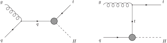
Figure 9: Feynman diagrams for $gq\to Ht$ via FCN couplings.

The $Ht$ process has a smaller cross section than $t\bar{t}$ with subsequent decay $\bar{t}\to H\bar{q}$ for the same values of $g_{tq}$, but also receives an additional contribution from the latter when $q$ is missed by the detector. This correction is not very significant for the analogous case of $Zt$ production, about $+10\%$ for the up quark and $+50\%$ for the charm, but in this case with $M_{H}>M_{Z}$ the additional contribution becomes more important. In our calculations we will then take into account both processes. The signals and backgrounds are generated as for the $l\nu bb\bar{b}j$ case. To estimate the number of events in which a jet is missed by the detector, we consider that a jet is missed when it has a low transverse momentum $p_{T}^{j}<20$ GeV or a very large pseudorapidity $\eta^{j}>3$.

The signal is reconstructed choosing first the pair of $b$ jets whose invariant mass is closest to $M_{H}$. The remaining $b$ jet is assigned to the decay of the top quark, whose mass is reconstructed as in the previous Section. To improve the signal to background ratio we use the kinematical cuts shown in Table 3.

Variable	Cut
$M_{H}^{\mathrm{rec}}$	115–125
$m_{t}^{\mathrm{rec}}$	160–190
$H_{T}$	$>220$

Table 3: Kinematical cuts for the $l\nu bb\bar{b}$ signal. The masses and the energy are in GeV.

In this case we cannot reduce the background imposing a veto cut to reject events in which a pair of jets has an invariant mass around $M_{W}$, because one of these jets is missed by the detector. Using an ANN does not improve the situation. The number of events for the $gu\to Ht$ and $gc\to Ht$ signals, the additional contribution $t\bar{t}\to Ht(q)$ and their backgrounds is collected in Table 4.

	Run L		Run H
	before	after	before	after
	cuts	cuts	cuts	cuts
$gu\to Ht$	57.2	35.1	470	293
$gc\to Ht$	11.9	6.8	95	56
$t\bar{t}\to Ht(q)$	42.1	22.0	170	186
$t\bar{t}$	1373	143	11260	1190
$Wb\bar{b}j$	77.2	1.6	619	12.7

Table 4: Number of $l\nu bb\bar{b}$ events before and after the kinematical cuts in Table 3 for the $Ht$ signal, the additional contribution $t\bar{t}\to Ht(q)$ and their backgrounds $t\bar{t}$ and $Wb\bar{b}j$. We use $g_{tq}=0.2$.

The limits obtained from the $Ht$ process are much less restrictive than from top decays. If no signal is observed, we obtain from Table 4 $g_{tu}\leq 0.13$, $g_{tc}\leq 0.19$ at Run L and $g_{tu}\leq 0.076$, $g_{tc}\leq 0.11$ at Run H. The same is true for Tevatron Run II, where the bounds obtained are very poor, $g_{tu}\leq 0.40$, $g_{tc}\leq 1.2$

4 LHC discovery potential

In the previous Sections we have considered that the signal is not seen, and have obtained 95% CL upper bounds on the size of the FCN couplings. These bounds imply the limits in the branching ratios of $t\to Hq$ in Table 5.

	LHC Run L		LHC Run H		Tevatron Run II
Signal	$\mathrm{Br}(t\to Hu)$	$\mathrm{Br}(t\to Hc)$	$\mathrm{Br}(t\to Hu)$	$\mathrm{Br}(t\to Hc)$	$\mathrm{Br}(t\to Hu)$	$\mathrm{Br}(t\to Hc)$
$l\nu bb\bar{b}j$	$1.4\times 10^{-4}$	$1.4\times 10^{-4}$	$4.5\times 10^{-5}$	$4.5\times 10^{-5}$	$5.2\times 10^{-3}$	$5.2\times 10^{-3}$
$l\nu bb\bar{b}$	$6.6\times 10^{-4}$	$1.3\times 10^{-3}$	$2.2\times 10^{-4}$	$4.3\times 10^{-4}$	$5.9\times 10^{-3}$	$5.3\times 10^{-2}$

Table 5: 95% CL upper limits on branching fractions of anomalous top decays obtained from the two processes analyzed. We also include the results for Tevatron Run II for comparison.

The limits obtained for different values of $M_{H}$ are very similar. For a lighter Higgs, the larger phase space (in the case of top decays) or the larger structure functions (in $Ht$ production) increase the signal cross section and hence allow a better determination of $g_{tq}$. This improvement disappears when expressing the limit in terms of a branching ratio. After repeating the analysis using $M_{H}=110$, $\mathrm{Br}(H\to b\bar{b})=0.8$, we find limits $3\%$ smaller from top decays and $5\%$ smaller from $Ht$ production. A heavier Higgs has the opposite behaviour, with the disadvantage of a smaller branching ratio $H\to b\bar{b}$. With $M_{H}=130$, $\mathrm{Br}(H\to b\bar{b})=0.45$ the limits from top decays and $Ht$ production are 1.5 and 1.3 times larger, respectively.

Let us turn now to the possibility of observing these anomalous decays. The most common criterion to estimate the discovery potential is to use the discovery significance defined as the ratio of the expected signal divided by the expected background fluctuation, $s\equiv n_{s}/\sqrt{n_{b}}$. This is adequate when $n_{b}>5$ and the Poisson distribution of the background can be approximated by a Gaussian with standard deviation $\sqrt{n_{b}}$. One has “evidence” ($3\,\sigma$) when $s>3$, and “discovery” ($5\,\sigma$) occurs with $s>5$.

In a general 2HDM, the most common ansatz for the FCN couplings is to assume that they scale with the quark masses. Under this assumption, the expected size of these couplings is $g_{tc}\simeq\sqrt{m_{t}m_{c}}/M_{W}=0.20$, $g_{tu}\simeq\sqrt{m_{t}m_{u}}/M_{W}=0.012$. An $Htc$ coupling of this size (leading to $\mathrm{Br}(t\to Hc)=1.5\times 10^{-3}$) will easily be detected and precisely measured. In top decays, at Run H we have $s=48$ using standard cuts and $s=68$ using the network cut. The benefit of the ANN is clear: the luminosity required to discover a signal is reduced to one half. In $Ht$ production, the significance is much smaller, $s=7$. The minimum coupling which can be discovered with $5\,\sigma$ is $g_{tc}=0.054$ ($\mathrm{Br}(t\to Hc)=1.1\times 10^{-4}$), and the minimum coupling which can be seen with $3\,\sigma$ is $g_{tc}=0.042$ ($\mathrm{Br}(t\to Hc)=6.5\times 10^{-5}$). An $Htu$ coupling $g_{tu}=0.012$ is too small to be seen, because in top decays we have only $s=0.23$, and in $Ht$ production $s=0.046$. Note that for a 2HDM this ansatz implies that there are other interesting FCN current processes, for instance $H\to\mu\tau$ at a muon collider [38].

Another possibility is to consider that the FCN couplings between two quarks are proportional to some CKM mixing angles involving these quarks. Rephasing invariance implies that these couplings are of the form $g_{qq^{\prime}}=\lambda V_{qi}V_{q^{\prime}i}^{*}$, with $i=d,s,b$ [5, 6]. Choosing $i=b$, the hierarchy among the mixing angles guarantees a small value for $g_{uc}=\lambda V_{ub}V_{cb}^{*}$. With $\lambda=5$ we recover the values of $g_{uc}$ and $g_{tc}$ of the previous ansatz, but $g_{tu}$ is a factor of two larger, $g_{tu}=0.025$. An Htu coupling of this size is now near the detectable level: $s=1.1$ in top decays and in $s=0.22$ in $Ht$ production, and if it is enhanced by a factor $\sim 2$ it would also be detected.

In models with exotic quarks the top FCN scalar couplings can be large, $g_{tu}\simeq 0.31$ or $g_{tc}\simeq 0.35$ (but not both simultaneously). These are the only models where the top can naturally have a large mixing with the up quark. However, the effects of top mixing in these models are most clearly seen with the appearance of tree level $Ztq$ couplings, leading to top anomalous decays $t\to Zq$ [39] and $Zt$ production [37]. If these processes are not observed at LHC, the $Htq$ couplings (proportional to the FCN $Ztq$ couplings) must be small, $g_{tu}\leq 0.024$, $g_{tc}\leq 0.030$, below the detectable level.

To analyze the case of top decays $t\to Hq$ in the MSSM it is necessary to recalculate the signal and backgrounds and train again the ANN with the new data. The reason is that in the region of parameters of interest the Higgs width is much larger due to the enhanced $Hbb$ coupling, and the $M_{H}^{\mathrm{rec}}$ distribution is broader in principle. For consistency we will use the parameters of Ref. [10]: $\tan\beta=35$, a pseudoscalar mass $M_{A}=120$ GeV and $c_{v}=c_{a}=1/\sqrt{2}$. With these parameters, the Higgs mass is in the interval $M_{H}=105-120$ GeV [40]. The kinematics is fairly independent of the particular value of $M_{H}$ used, as we have shown above, the only difference being the Higgs decay rate to $b\bar{b}$ which varies slightly in this mass range. For our analysis we take $M_{H}=110$ GeV, $\mathrm{Br}(H\to b\bar{b})=0.9$ [41]. Our limits on $\mathrm{Br}(t\to Hq)$ are proportional to $1/\mathrm{Br}(H\to b\bar{b})$. To separate signal from background we select events with network output $r>0.994$.

There are large regions in the MSSM parameter space where $\mathrm{Br}(t\to Hc)$ is greater than $1.1\times 10^{-4}$ and even reaches $4\times 10^{-4}$ [10]. These decays can be discovered at LHC Run H with $5\,\sigma-18\,\sigma$. Also, a rate $\mathrm{Br}(t\to Hc)=6.7\times 10^{-5}$ is observable with $3\,\sigma$. The decays $t\to Hu$ have a too small rate to be seen.

On the other hand, if no signal is observed we obtain a limit $g_{tq}\leq 0.054$ at Run L and $g_{tq}\leq 0.031$ at Run H. Note that although these limits seem better than those obtained for $M_{H}=120$, when translated into branching ratios they give very similar bounds, $\mathrm{Br}(t\to Hq)\leq 1.4\times 10^{-4}$ at Run L and $\mathrm{Br}(t\to Hq)\leq 4.7\times 10^{-5}$ at Run H.

References

- [1] S. Glashow and S. Weinberg, Phys. Rev. D15, 1958 (1977)
- [2] D. Atwood, L. Reina and A. Soni, Phys. Rev. D55, 3156 (1997)
- [3] F. del Aguila and M. J. Bowick, Phys. Lett. 169B, 144 (1982)
- [4] T. P. Cheng and M. Sher, Phys. Rev. D35, 3484 (1987)
- [5] A. S. Joshipura and S. D. Rindani, Phys. Lett. B260, 149 (1991)
- [6] G. C. Branco, W. Grimus and L. Lavoura, Phys. Lett. B380, 119 (1996)
- [7] F. del Aguila and M. J. Bowick, Nucl. Phys. B224, 107 (1983); for a recent analysis see K. Higuchi and K. Yamamoto, Phys. Rev. D62, 073005 (2000)
- [8] F. del Aguila, J. A. Aguilar-Saavedra and R. Miquel, Phys. Rev. Lett. 82, 1628 (1999); see also F. del Aguila and J. A. Aguilar-Saavedra, hep-ph/9906461
- [9] J.-M. Yang and C.-S. Li, Phys. Rev. D49 3412 (1994)
- [10] J. Guasch and J. Solà, Nucl. Phys. B562, 3 (1999)
- [11] B. Mele, S. Petrarca and A. Soddu, Phys. Lett. B435, 401 (1998)
- [12] B. A. Dobrescu and C. T. Hill, Phys. Rev. Lett. 81, 2634 (1998); R. S. Chivukula, B. A. Dobrescu, H. Georgi and C. T. Hill, Phys. Rev. D59, 075003 (1999)
- [13] D. Delepine, J. M. Gerard and R. Gonzalez Felipe, Phys. Lett. B372, 271 (1996)
- [14] G. Burdman, Phys. Rev. Lett. 83, 2888 (1999)
- [15] H.-J. He and C.-P. Yuan, Phys. Rev. Lett. 83, 28 (1999); H.-J. He, T. Tait and C.-P. Yuan, Phys. Rev. D62, 011702 (2000)
- [16] For a review see M. Beneke, I. Efthymipopulos, M. L. Mangano, J. Womersley (conveners) et al., report in the Workshop on Standard Model Physics (and more) at the LHC, Geneva, hep-ph/0003033
- [17] S. Bar-Shalom, G. Eilam, A. Soni and J. Wudka, Phys. Rev. Lett. 79, 1217 (1997)
- [18] D. Atwood, L. Reina and A. Soni, Phys. Rev. Lett. 75, 3800 (1995)
- [19] D. Abbaneo et al., CERN-EP-2000-016; P. Langacker, hep-ph/9905428
- [20] M. Carena, M. Quiros and C.E.M. Wagner, Nucl. Phys. B461, 407 (1996)
- [21] The LEP Collaborations ALEPH, DELPHI, L3 and OPAL, CERN-EP-2000-055
- [22] W.-S. Hou, Phys. Lett. B296, 179 (1992)
- [23] W.-S. Hou, G.-L. Lin, C.-Y. Ma and C.-P. Yuan, Phys. Lett. B409, 344 (1997)
- [24] SLD Collaboration, K. Abe et al., Phys. Rev. Lett. 80, 660 (1998)
- [25] E. Murayama, I. Watanabe and K. Hagiwara, KEK report 91-11, January 1992
- [26] T. Stelzer and W. F. Long , Comput. Phys. Commun. 81, 357 (1994)
- [27] R. K. Ellis, Phys. Lett. B 259, 492 (1991); P. Nason, S. Dawson and R. K. Ellis, Nucl. Phys. B303, 607 (1988); W. Beenakker et al., ibid. B351, 507 (1991)
- [28] F. Berends, H. Kuijf, B. Tausk and W. Giele, Nucl. Phys. B357, 32 (1991)
- [29] R. Hamberg, W.L. van Neerven and T. Matsuura, Nucl. Phys. B359, 343 (1991)
- [30] A. D. Martin, R. G. Roberts, W. J. Stirling and R. S. Thorne, Eur. Phys. J. C4, 463 (1998);
- [31] See for instance I. Efthymiopoulos, Acta Phys. Polon. B30, 2309 (1999)
- [32] ATLAS Trigger Performance - Status Report CERN/LHCC 98-15
- [33] C. Peterson, T. Rognvaldsson and L. Lonnblad, Comput. Phys. Commun. 81, 185 (1994)
- [34] G. J. Feldman and R. D. Cousins, Phys. Rev. D57, 3873 (1998)
- [35] J. A. Aguilar-Saavedra, Comput. Phys. Commun. 130, 190 (2000)
- [36] W. J. Stirling and D. J. Summers, Phys. Lett. B283, 411 (1992); G. Bordes and B. van Eijk, Phys. Lett. B299, 315 (1993)
- [37] F. del Aguila, J. A. Aguilar-Saavedra and Ll. Ametller, Phys. Lett. B462, 310 (1999); F. del Aguila and J. A. Aguilar-Saavedra, Nucl. Phys. B576, 56 (2000)
- [38] M. Sher, Phys. Lett. B487, 151 (2000)
- [39] T. Han, R. D. Peccei and X. Zhang, Nucl. Phys. B454, 527 (1995)
- [40] S. Heinemeyer, W. Hollik and G. Weiglein, Phys. Lett. B440, 296 (1998); S. Heinemeyer, W. Hollik and G. Weiglein, Phys. Lett. B455, 179 (1999)
- [41] S. Heinemeyer, W. Hollik and G. Weiglein, Eur. Phys. J. C16, 139 (2000)