CP3-13-26
Top-quark decay into Higgs boson and a light quark at next-to-leading order in QCD
Abstract
Neutral flavor-changing transitions are hugely suppressed in the Standard Model and therefore they are very sensitive to new physics. We consider the decay rate of where using an effective field theory approach. We perform the calculation at next-to-leading order (NLO) in QCD including the relevant dimension-six operators. We find that at NLO the contribution from the flavor-changing chromomagnetic operator is as important as the standard QCD correction to the flavor-changing Yukawa coupling. In addition to improving the accuracy of the theoretical predictions, the NLO calculation provides information on the operator mixing under the renormalization group.
pacs:
12.38.Bx,14.65.Ha,14.80.BnI Introduction
The discovery of a particle of about 125 GeV mass Chatrchyan et al. (2012); Aad et al. (2012) that resembles the Higgs boson of the Standard Model (SM) Englert and Brout (1964); Higgs (1964); Weinberg (1976) has opened a new era in particle physics. A new realm of possibilities for exploring the electroweak breaking sector and new exciting opportunities to search for new physics in general have appeared. From the existence of new symmetries to new space-time dimensions, from new matter to a richer scalar sector, many are still viable options. For instance, extra scalar states could exist mostly (or exclusively) coupling to the Higgs boson or new particles could decay into final states involving the SM scalar boson. In addition to direct searches, the accurate measurement of the coupling strengths and structures to the SM particles could point to the scale of new physics.
In this perspective, the study of neutral-flavor-changing (NFC) couplings involving the top quark and the Higgs boson is of special interest. In the Standard Model, NFC interactions are absent at tree level and hugely suppressed by the Glashow-Iliopoulos-Maiani mechanism at one loop. Finding evidence for such processes taking place at measurable rates would basically always imply new physics not too far from the TeV scales. The recently observed excess of Lees et al. (2012) could hint to NFC mediated by the Higgs boson Crivellin et al. (2012).
In this work we consider the decay of a top quark into a light (up or charm) quark and the Higgs boson, assuming new physics residing at a scale . The SM contribution to the branching ratio is extremely small, at order – Eilam et al. (1991); Mele et al. (1998); Aguilar-Saavedra (2004). Indirect bounds on branching ratio have been set, for example, in Refs. Larios et al. (2005); Aranda et al. (2010), and are found to be at level. Collider searches for these interactions have been discussed in Aguilar-Saavedra and Branco (2000); Aguilar-Saavedra (2004); Kao et al. (2012); Wang et al. (2012); Atwood et al. (2013). The first limit at LHC, , was given in Craig et al. (2012).
In this Letter we present the calculation at next-to-leading order (NLO) in QCD of the inclusive top-quark decay into a Higgs boson via NFC interactions in an effective field theory (EFT) Weinberg (1979) approach. We consider all lowest dimensional operators compatible with the symmetries of the SM,
| (1) |
where represents the scale of new physics. Our calculation completes the set of NLO results available for 2-body top decays, such as and with Drobnak et al. (2010a, b, c); Zhang et al. (2010), which we have independently checked.
II SETUP
A complete and minimal list of dimension-six operators that can be written with SM fields and are compatible with the symmetries of the SM can be found in Ref. Grzadkowski et al. (2010). We use the same operator basis, employing the following notation for quark fields:
and . There are two main Lorentz structures that contribute to the decay, the dimension-six Yukawa interaction , and the chromomagnetic operator . The latter contributes only at NLO. Considering the possible flavor assignments, they read
| (2) | |||
| (3) | |||
| (4) | |||
| (5) |
where superscript and denote the flavor structure. The Hermitian conjugates of the operators contribute to with the opposite chirality of the corresponding operators. In addition, replacing the up-quark field with the charm-quark field gives the same set of operators with and flavor structures.
Note that the operators have been normalized by attaching appropriate factors of the top-quark Yukawa coupling and the strong coupling . The powers of these factors are determined by requiring that, whenever these operators give rise to a SM-like vertex, the coupling strength relative to the SM coupling is always one of the following factor:
| (6) |
where is the typical energy of the particles entering the vertex. This helps to determine the order of the mixing between these operators. With this convention, the operator mixing induced by a gluon exchange is always of order , even if the gluon vertex comes from an effective operator. In fact the normalization coefficient of these operators depends on the details of the full theory beyond . In short our convention states that for any bilinear quark operators, we attach a to each Higgs field, and a for each gluon field. We remark that in this work we choose to be defined in terms of the on-shell top-quark mass
| (7) |
This is just for simplicity. As a result, it does not contribute to the anomalous dimension of the operators at order .
In the following we focus on operators with and flavor structure. The extension of the results from to is trivial. In addition, since there is no mixing between operators of type and we can omit the superscripts and , and only consider the case. Results for can be obtained by flipping the chirality of the quarks.
At the tree level, only contributes. The effective Lagrangian describing the interaction of a top quark, a light quark and the Higgs boson reads
| (8) |
In addition, the terms in involving the vacuum expectation value of the Higgs field give rise to mixing. The standard way to deal with this effect is to perform a set of transformations that diagonalize the mass matrix:
| (9) | |||
| (10) |
and similarly for . As a result Eq. (8) is modified and the interaction reads
| (11) |
Equivalently, one can add a dimension-four counterterm such that the operator becomes
| (12) |
and the mixing term disappears.
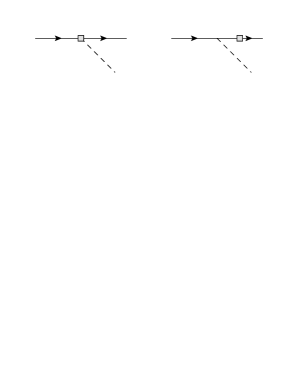
Another possibility is to keep the quark fields not diagonal, and simply include the external leg corrections to the diagrams, as shown in Fig. 1. This gives the same result for . At the one-loop level, we choose this point of view to take into account the loop-induced mixing.
The decay rate up to next-to-leading corrections in the strong coupling can be written as
| (13) |
with LO result Hou (1992)
| (14) |
where the light quark mass is neglected.
III NLO calculation strategy
We briefly describe our strategy for the computation of NLO corrections in QCD to the decay rate.
First, we aim at NLO accuracy in QCD but only LO in EFT expansion. Calculation of higher orders of requires complete knowledge of dimension-eight operators, and it is beyond the scope of this paper. As there are no SM FCNC decays at LO, the first nonzero contribution to the decay width from new physics is order .
To regulate both ultraviolet (UV) and infrared (IR) divergences, we employ dimensional regularization ’t Hooft and Veltman (1972) and work in dimensions. Whenever is present in our computation, we use the following prescription based on the ’t Hooft-Veltman scheme Larin (1993); Ball and Zwicky (2005):
| (15) | |||
| (16) | |||
| (17) |
where .
IR divergences cancel between virtual and real diagrams when sufficiently inclusive observables are considered. The rest of the calculation involves the following:
-
1.
a UV-divergent part, which gives rise to operator mixing and renormalization group equations,
-
2.
UV-finite part, which gives the actual corrections to the matrix elements.
In the first step, we calculate the UV-divergent part arising from the loop diagrams, and identify the UV counterterms by applying the scheme and requiring that the UV-divergent terms cancel. The outcome of this procedure is a set of counterterms for dimension-six operators. We then proceed to work out the anomalous dimension and the renormalization group equations of these operators. These equations can be used to evolve the coefficients of these operators from a higher scale down to the scale of top-quark mass.
In the second step, we calculate the UV-finite part. The final result is given in terms of the coefficients of these operators defined at the scale of top-quark mass.
Throughout this paper we ignore the light quark masses, and assume .
IV Operator renormalization
The following counterterms for the SM part are used. For the external fields:
| (18) | |||
| (19) | |||
| (20) | |||
| (21) |
while for the couplings:
| (22) | |||
| (23) |
where . This set of counterterms corresponds to renormalizing the external fields and the top Yukawa coupling on shell, and the strong coupling in the scheme. We consider five light flavors in the running of . We then apply the scheme to the dimension-six operators and require that dimension-six operators only mix with dimension-six operators. The counterterms are given by
| (24) |
We first consider . Including counterterms, the Lagrangian can be written as
| (25) | ||||
| (26) | ||||
| (27) |
where the counterterm is
| (28) |
where the dots stand for additional finite terms. The renormalization mirrors that of the SM Yukawa terms. is determined by the part of the two-point () and three-point () functions. We find
| (29) |
Now we consider . The vertex is given by
| (30) |
This gives rise to a mixing at one loop. We find
| (31) |
The first term in the bracket implies
| (32) |
One could also determine this counterterm by calculating the three-point () function. The pole in the second term can be dealt through the following dimension-six counterterms:
| (33) | |||
| (34) |
However, these operators vanish when the equations of motions are considered (on-shell or off-shell quark does not matter). Therefore one can simply ignore these operators as the poles always cancel out when combining with the vertex contributions in a physical amplitude.
Finally, the renormalization of requires computation of at one loop. We find:
| (35) |
while is zero because there is no contribution from to at one loop at order .
In summary, we have the following anomalous dimension matrix for and
| (36) |
The operator can also renormalize other operators. The complete operator mixing can be extracted from the calculation of . However, at order no other operator can renormalize and , so for the process the anomalous dimensions given in Eq. (36) are sufficient.
V Finite corrections
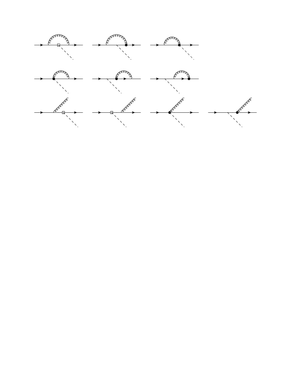
We proceed to carry out the UV-finite part of the calculation. At NLO, the loop corrections and real corrections are shown in Fig. 2. To simplify the calculation, we rotate the and quark fields to remove the mixing due to . More specifically, given the following effective Lagrangian,
| (37) |
we perform the following rotation:
| (38) | |||
| (39) |
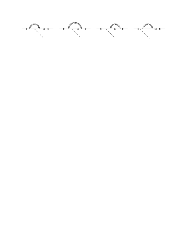
As a result the mixing due to the first term in Eq. (37) is removed; therefore, only the vertex correction needs to be considered for . On the other hand, for , the second terms in Eq. (37) contains a mixing counterterm that is not rotated away. This term cancels the UV-divergent terms from at one loop in mixing. The remaining finite part is included in the leg correction diagrams in Fig. 2. Because the rotation of fields is of order , and the LO contribution to is already of order , the rotation does not affect our results. As a check, we have computed the loop corrections without redefining the fields. In this case there are four more diagrams, as shown in Fig. 3.
Including both virtual and real corrections, the total NLO correction to the decay rate is () :
| (40) |
The term does not have a dependence. This is because the tree-level amplitude does not have a contribution from . As a result, the term entirely comes from real corrections (virtual corrections are interferences between tree- and one-loop level amplitudes), and it is independent of .
In addition, the term contains which is divergent in the limit . This corresponds to a soft Higgs emission which in the limit is divergent when . In this limit, we have
| (41) |
As this term is purely from the real corrections, it can be thought of as the real Higgs emission correction to the decay mode . The soft divergence is expected to be canceled by the wave function renormalization of the top quark in the process , coming from a virtual Higgs bubble diagram. As a check, we have computed this diagram and find
| (42) |
The corresponding contribution to the virtual correction to the decay width of is
| (43) |
which exactly cancels the term in Eq. (41).
The other two terms in , and Re() do not have this divergence. In particular, the interference term [which is proportional to Re()] is finite in the limit, even though it contains terms and functions. This is because the two real correction diagrams from cancel each other when .
VI Numerical analysis
For the numerical analysis we assume TeV. For the input parameters, we use Beringer et al. (2012)
| (44) | ||||
| (45) | ||||
| (46) |
With these parameters we find
| (47) | ||||
| (48) |
The term is 4 orders of magnitude smaller than the other two terms, and thus it is interesting to understand such a suppression. As we have mentioned, this term only receives contributions from real emission. We find that, due to the structure of the coupling from , the squared amplitude for depends on . We find
| (49) |
where and .
As a result, this term is dominated by the phase space region where is large. However, the maximum value of is and is therefore suppressed for a large Higgs mass. In fact, for GeV this suppression factor for already reaches the level. The phase space itself accounts for one additional order of magnitude, so the total decay width from is small for GeV. On the other hand, the other two terms [ and Re()] are not affected by this factor as their main contribution comes from virtual topologies.
We now consider the impact of the NLO corrections to phenomenological applications. In the following we assume both and to be real. At order the contribution from is even more important than that from . Neglecting the term, the ratio between NLO and LO result is
| (50) |
at . Here we have used , which we obtain with the program RunDec Chetyrkin et al. (2000) from the value =0.1184 Beringer et al. (2012). Without the QCD correction is about , while if and are similar in size, the QCD correction can reach the level.
The residual theoretical uncertainties can be estimated by checking the scale dependence of the decay width. Using the anomalous dimension matrix given in Eq. (36), we solve the scale dependence of the coefficients and :
| (51) | ||||
| (52) |
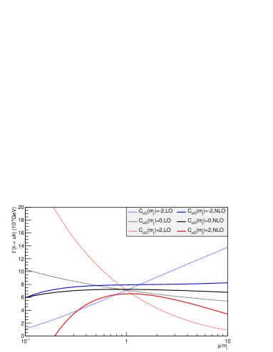
where . The running of is affected by the operator . In Fig. 4, we show the dependence of both LO and NLO results for the width, with different values of . We can see that the renormalization scale dependence at LO can be quite large depending on the value of , and that it is greatly reduced at NLO in QCD.
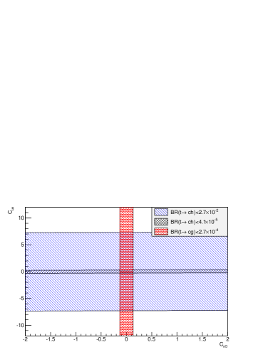
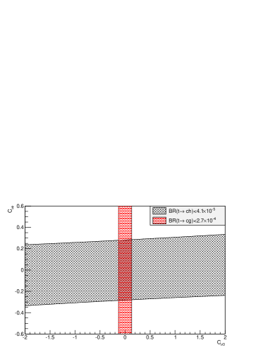
Finally, for the sake of illustration, in Fig. 5 we plot the limits on and plane. The region in the parameter space corresponding to the current bound BR from CMS Craig et al. (2012) is shown, as well as the upper limit for as estimated in Ref. Aguilar-Saavedra (2004), i.e. BR for an integrated luminosity of 100 . In our results, the term has been neglected and the next-to-next-to-leading-order top quark width result Czarnecki et al. (2010) is used. The constraints on coming from BR Cristinziani (2013) are also shown.
VII Conclusion
We have presented a calculation for the decay width of in the EFT approach at NLO in QCD. Two operators contribute at LO, while at NLO two additional operators (and their mixing) need to be included. We find that QCD correction can reach the 10% level, depending on the relative size of these operators. The possibly large scale dependence of the LO results is tamed at NLO.
VIII Acknowledgements
This work is supported by the IISN “Fundamental interactions” convention 4.4517.08. and in part by the Belgian Federal Science Policy Office through the Interuniversity Attraction Pole P7/37.
References
- Chatrchyan et al. (2012) S. Chatrchyan et al. (CMS Collaboration), Phys.Lett. B716, 30 (2012), eprint 1207.7235.
- Aad et al. (2012) G. Aad et al. (ATLAS Collaboration), Phys.Lett. B716, 1 (2012), eprint 1207.7214.
- Englert and Brout (1964) F. Englert and R. Brout, Phys.Rev.Lett. 13, 321 (1964).
- Higgs (1964) P. W. Higgs, Phys.Rev.Lett. 13, 508 (1964).
- Weinberg (1976) S. Weinberg, Phys.Rev. D13, 974 (1976).
- Lees et al. (2012) J. Lees et al. (BaBar Collaboration), Phys.Rev.Lett. 109, 101802 (2012), eprint 1205.5442.
- Crivellin et al. (2012) A. Crivellin, C. Greub, and A. Kokulu, Phys.Rev. D86, 054014 (2012), eprint 1206.2634.
- Eilam et al. (1991) G. Eilam, J. Hewett, and A. Soni, Phys.Rev. D44, 1473 (1991).
- Mele et al. (1998) B. Mele, S. Petrarca, and A. Soddu, Phys.Lett. B435, 401 (1998), eprint hep-ph/9805498.
- Aguilar-Saavedra (2004) J. Aguilar-Saavedra, Acta Phys.Polon. B35, 2695 (2004), eprint hep-ph/0409342.
- Larios et al. (2005) F. Larios, R. Martinez, and M. Perez, Phys.Rev. D72, 057504 (2005), eprint hep-ph/0412222.
- Aranda et al. (2010) J. Aranda, A. Cordero-Cid, F. Ramirez-Zavaleta, J. Toscano, and E. Tututi, Phys.Rev. D81, 077701 (2010), eprint 0911.2304.
- Aguilar-Saavedra and Branco (2000) J. Aguilar-Saavedra and G. Branco, Phys.Lett. B495, 347 (2000), eprint hep-ph/0004190.
- Kao et al. (2012) C. Kao, H.-Y. Cheng, W.-S. Hou, and J. Sayre, Phys.Lett. B716, 225 (2012), eprint 1112.1707.
- Wang et al. (2012) Y. Wang, F. P. Huang, C. S. Li, B. H. Li, D. Y. Shao, et al., Phys.Rev. D86, 094014 (2012), eprint 1208.2902.
- Atwood et al. (2013) D. Atwood, S. K. Gupta, and A. Soni (2013), eprint 1305.2427.
- Craig et al. (2012) N. Craig, J. A. Evans, R. Gray, M. Park, S. Somalwar, et al., Phys.Rev. D86, 075002 (2012), eprint 1207.6794.
- Weinberg (1979) S. Weinberg, Physica A96, 327 (1979).
- Drobnak et al. (2010a) J. Drobnak, S. Fajfer, and J. F. Kamenik, Phys.Rev. D82, 114008 (2010a), eprint 1010.2402.
- Drobnak et al. (2010b) J. Drobnak, S. Fajfer, and J. F. Kamenik, Phys.Rev.Lett. 104, 252001 (2010b), eprint 1004.0620.
- Drobnak et al. (2010c) J. Drobnak, S. Fajfer, and J. F. Kamenik, Phys.Rev. D82, 073016 (2010c), eprint 1007.2551.
- Zhang et al. (2010) J. J. Zhang, C. S. Li, J. Gao, H. X. Zhu, C.-P. Yuan, et al., Phys.Rev. D82, 073005 (2010), eprint 1004.0898.
- Grzadkowski et al. (2010) B. Grzadkowski, M. Iskrzynski, M. Misiak, and J. Rosiek, JHEP 1010, 085 (2010), eprint 1008.4884.
- Hou (1992) W.-S. Hou, Phys.Lett. B296, 179 (1992).
- ’t Hooft and Veltman (1972) G. ’t Hooft and M. Veltman, Nucl.Phys. B44, 189 (1972).
- Larin (1993) S. Larin, Phys.Lett. B303, 113 (1993), eprint hep-ph/9302240.
- Ball and Zwicky (2005) P. Ball and R. Zwicky, Phys.Rev. D71, 014029 (2005), eprint hep-ph/0412079.
- Beringer et al. (2012) J. Beringer et al. (Particle Data Group), Phys.Rev. D86, 010001 (2012).
- Chetyrkin et al. (2000) K. Chetyrkin, J. H. Kuhn, and M. Steinhauser, Comput.Phys.Commun. 133, 43 (2000), eprint hep-ph/0004189.
- Czarnecki et al. (2010) A. Czarnecki, J. G. Korner, and J. H. Piclum, Phys.Rev. D81, 111503 (2010), eprint 1005.2625.
- Cristinziani (2013) M. Cristinziani (ATLAS Collaboration) (2013), eprint 1302.3698.