hep-ph/0703031

BRIDGE:
Branching Ratio Inquiry/Decay Generated Events

Patrick Meade^a and Matthew Reece^b

^aJefferson Physical Laboratory
Harvard University, Cambridge, MA 02138, USA

^bInstitute for High Energy Phenomenology
Newman Laboratory of Elementary Particle Physics
Cornell University, Ithaca, NY 14853, USA

We present the manual for the program BRIDGE: Branching Ratio Inquiry/Decay Generated Events. The program is designed to operate with arbitrary models defined within matrix element generators, so that one can simulate events with small final-state multiplicities, decay them with BRIDGE, and then pass them to showering and hadronization programs. BRI can automatically calculate widths of two and three body decays. DGE can decay unstable particles in any Les Houches formatted event file. DGE is useful for the generation of event files with long decay chains, replacing large matrix elements by small matrix elements followed by sequences of decays. BRIDGE is currently designed to work with the MadGraph/MadEvent programs for implementing and simulating new physics models. In particular, it can operate with the MadGraph implementation of the MSSM. In this manual we describe how to use BRIDGE, and present a number of sample results to demonstrate its accuracy.

1 Introduction

In recent years the workhorses of Monte Carlo event generation, parton showering, and hadronization, Pythia [1] and Herwig [2], have begun to offload some of their duties to other programs. It is now possible to define new models, automatically generate matrix elements, and simulate parton-level events using a variety of available packages (among them CompHEP/CalcHEP [3, 4], MadGraph [5], AcerMC [6], Amegic++ [7], and Grace [8]). The events simulated in these packages can then be passed to the next step in the chain, a parton-shower code, using a standardized “Les Houches Accord” file format [9, 10].

These developments (and others; we apologize for the many software packages we cannot mention in this brief summary) have made the task of implementing a model of new physics and studying its collider signatures far easier than it has been in the past. On the other hand, in our experience there have been two bottlenecks in the process, which demanded a general solution. In BRIDGE we provide (at least a useful first approximation to) that solution.

The first is that in order to accurately calculate matrix elements, one wants to know the widths of new unstable particles in the model. There exist specialized tools (e.g. HDECAY [11], SDECAY [12], and SUSY-HIT [13]) for particular models. There is also a general calculator in CompHEP [3] (and its spin-off, CalcHEP [4]), but to use it with another event generator one must translate the entire model into CompHEP’s formats. It seemed desirable to have a general, independent calculator of tree-level decay widths. BRIDGE can currently read MadGraph-style definitions of particles and interactions and use them to calculate widths, but it can easily be extended to read input in other formats as well.

The main advantage of BRIDGE over CompHEP/CalcHEP as a width calculator is that it adds decay functionality, which overcomes the second bottleneck. The problem is simulating events that involve long decay chains, which are familiar in the MSSM context (e.g. decays of squarks or gluinos) but also arise in many other models of more recent vintage. In an ideal world we would all have enough computing power to integrate a full $2\rightarrow N$ phase space where $N$ could be as large as 8 or 10. Unfortunately, practical limitations on computer power make it desirable to be able to simulate $2\rightarrow 2$ or $2\rightarrow 4$ processes and then decay the unstable final-state particles. This factorizes the matrix elements, and one loses information both to narrow-width approximations and to the loss of interference effects, but for most purposes it seems to be a fairly good approximation and it greatly speeds up computations. However, there has not been a general code that can decay unstable particles for arbitrary models and keep the original helicity structure of the vertex (i.e., go beyond a flat phase space approximation). BRIDGE provides that code.

BRIDGE operates in two pieces, “BRI” (Branching Ratio Inquiry, though it really calculates widths) and “DGE” (Decay Generated Events). The BRI stage uses Vegas integration [14] of the phase space for the decay to calculate a width. The amplitudes are computed using the HELAS libraries [15]. The DGE stage uses the stored grids from BRI to choose random points in the phase space to use to decay actual events. BRIDGE owes much to Fabio Maltoni’s “DECAY” code included in MadGraph, which plays a similar role but only for Standard Model particles.

In Section 2 we will describe the structure of the program and how to use it. In Section 3 we will show a variety of examples of calculations performed with BRIDGE and compared to known answers or to simulations with full matrix elements.

2 Program Structure and Use

In this section we will discuss how BRIDGE should be “installed” and how to run BRI and DGE. We will also briefly discuss how the program works, for the benefit of the user who might wish to read or modify the source code. The implementation of BRIDGE is in C++ and is driven by several classes which allow BRIDGE to easily accommodate any model. In addition to the basic classes there are several input/output functions that are driven by the user’s interactive choices in the executables runBRI.exe or runDGE.exe.

The program BRIDGE comes packaged inside a tarball BRIDGEvX.XX.tar.gz that should be unzipped and untarred in the main Madgraph directory (e.g. MG_ME_V4.1.xx/). This relative location is used to find the HELAS libraries and the model file directories in MG4. After untarring BRIDGE you will have a directory MG_ME_V4.1.xx/BRIDGE that includes the subdirectories source, input and results. All files relevant to generating the BRI and DGE executables are located within the source directory, and the input directory has several model files associated with the SM and MSSM for examples. To generate the executables associated with BRIDGE simply run make from the main BRIDGE directory. The makefile will create the two executables previously mentioned, as well as runBRIsusy.exe or runDGEsusy.exe which will be discussed in Section 3.3. Additionally beyond the described functions, from v2.0 there are additional batch modes for all executables that will be described in Section 2.3.

2.1 BRI

BRI is designed such that given a definition of a model, including numerical values for couplings and masses, all two and three body partial widths can be calculated within that model at tree level. By default only the standard renormalizable vertices are included, via the HELAS libraries. In addition it is also possible to include loop decays if implemented by the user. An example will be given in Section 3.4.

When runBRI.exe is run, it first parses the model files for all particles and interactions in a given model. It then will parse the files associated with the numerical couplings and masses. From this definition of a model it will construct all possible kinematically allowed two and three body decays for a given particle. At this point the user provides information on which particles they want BRI to calculate the appropriate widths for. BRI then calculates the widths by integration, using the Vegas algorithm [14]. BRI also stores the grids generated by Vegas so that they can be reused when decaying particles with DGE.

The actual implementation that BRI uses is based upon the use of MG4 model definitions and the HELAS library for setting up the matrix elements. The Madgraph model definitions involve minimal syntax. There is a particles.dat which simply lists a particle name and its relevant properties (e.g. antiparticle name, name of a parameter that stores its mass, etc.), and an interactions.dat which contains a list of vertices and a name for the relevant coupling. We refer to the Madgraph documentation [5] for details.

The real work in defining the model is to provide the numerical values for all of the couplings in the model. BRI can read a simple text file containing a list of coupling names (which should match that specified in interactions.dat) followed by up to four numbers. If one number is specified, it is taken to be a real parameter. If two are specified, it is a complex parameter; the first number is the real part, the second the imaginary part. Finally, couplings involving fermions require four real parameters to specify: the first two are the real and imaginary parts of the left-handed coupling, and the latter two are the real and imaginary parts of the right-handed coupling. For example, here are a few lines from the default Standard Model file SMparams.txt:

WMASS 80.419
G 1.228
GG -1.228 0.0 -1.228 0
gzzhh       0.27638     0.00000
gal       0.31345      0.00000       0.31345      0.00000

Note that extra whitespace is ignored (but each coupling should be on its own line), and the coupling name is case-insensitive.

There is unfortunately not a universal format for a “model” of physics beyond the standard model, but the MG4 collaboration has provided a relatively easy-to-use and well-defined format in their example models and their “usrmod” which is designed to easily incorporate user implemented models. We have elected to choose their formats for use in BRIDGE, but in principle our code can operate with other formats if the relevant input/output code is added. Additionally, as will be further discussed in Section 2.1.1, the Madgraph collaboration has provided a utility to numerically generate the list of couplings for any user implemented model through their usrmod in the format that BRIDGE reads.

2.1.1 Running BRI

The runBRI.exe executable has two modes of operation. The first is designed to seamlessly interface with the Madgraph 4 usrmod. The user must specify the model directory name, and BRI will find the appropriate files there. Alternatively, the user can specify all the necessary input files as well as the location where the results will be placed.

We first describe the working of the more interactive mode. There are three files that are requested by runBRI.exe. The first two are the definitions of a model in Madgraph form, i.e. files in the format of particles.dat and interactions.dat. The third is the file that includes the numerical values of the couplings and masses in the model, an example of which is given for the SM in BRIDGE/input/SMparams.txt. The next step is to determine the list of particles for which widths are to be computed and grids to be made. The user is then presented with a list of all particles available for calculation, and prompted to choose either a subset of these particles or to calculate decays of all of them. By default the widths are calculated only for a particle, not for its antiparticle, although you can also ask for the antiparticle decay when specifying the list of particles to decay. When DGE decays event files, it needs decay tables and grids for the antiparticles as well. For that purpose we provide a script, antigrids.pl, which will symbolically link the tables for antiparticles to those for particles. (We explain more about the operation of this script in the first paragraph of Section 2.2.) Once the particles to be decayed are determined, the user is prompted to specify input parameters for the Vegas integration. The user is asked for a seed for the random number generator for Vegas (the default is the time) and additionally the number of calls (the default is 50000) and of iterations (the default is 5). Calculating the decays is the most computationally intensive part of BRIDGE, so if you are calculating a large number of particles, be careful in your choice of number of calls! At this point BRI loops over the particles requested and calculates all two and three body decays for the given particle. For each particle a file "particle name"_decays.table is created with a table of branching ratios for the particle’s decays. Additionally for every decay mode of the particle there is a corresponding ".grid" file from Vegas created with a filename that has the parent particle and the corresponding daughters in the filename. These files will be used by DGE when decaying the particles. Also, a decay table of all particles is written to a file of your choosing in Les Houches format [10].

The alternate run mode of BRI uses a specified Madgraph usrmod directory. The tools in usrmod can take the work in generating a file with numerical couplings out of the user’s hands. When using this mode of BRI the user is required to have implemented the model in Madgraph exactly as the “usrmod” instructions explain. Additionally one will have to have run make couplings in the usrmod directory and then run the executable couplings which makes a file couplings_check.txt. This file will have numerically evaluated all couplings for the Madgraph model and thus the user is not required to have made a numerical couplings file as they would have in the interactive mode. Additionally the user is required to have edited the file param_card.dat to include the numerical values of the masses of the new particles. One should note that this requires the user to do nothing more than they would have for any implementation in Madgraph. When executing BRI with the Madgraph usrmod all one specifies is the name of the Madgraph model directory, and then the execution is identical to the other mode of running BRI. The only other difference in the Madgraph running mode is that the output has an additional feature. For any particles whose decays are calculated by BRI in this mode, the widths for the particles are updated in the param_card.dat for the model, so that after executing runBRI.exe in this mode one can run Madgraph with the correct widths automatically implemented.

2.2 DGE

We will now describe the working of DGE. The program DGE is based primarily upon the original decay program included in Madgraph, written by Fabio Maltoni. The original decay program for Madgraph was hard wired to the Standard Model and each particular decay for an SM particle was implemented separately. The main difference in DGE is that it is “model-independent” and automatically will search for all possible decays for the particles of a given model. To run DGE it is first necessary to have executed runBRI.exe before runDGE.exe so as to have generated all the necessary Vegas grids that DGE will use. If you created grids for a particle but not its antiparticle (the default), you should run antigrids.pl. The script takes two command line arguments. The first is the path to the particles.dat so that the script can learn which particle name is associated to which antiparticle name. The second is the path to the results directory where the grids are located. The script will then copy each existing decay table to one appropriate for the antiparticle, provided this does not already exist. It will also symbolically link the grids for the antiparticle to those for the particle.

DGE will again prompt you for the input files, just as BRI did. Then it will ask for an input events file. (Currently, BRIDGE has only been tested on MadEvent output files. If you need to use it with the output of some other event generator, you either need to make sure the format matches, edit the BRIDGE code yourself, or contact us for assistance.) You will then be asked for a name for the output events file, and the directory where the BRI grids are stored. Also, you will again be prompted for a random number seed which defaults to the current time.

DGE will give you three different options for what to do with the input file:

  Choose a mode:
    1. Decay a particular particle.
    2. Decay down to a set of final-state particles.
    3. Decay using a specified set of decay modes.

In mode 1, you specify some particle to decay. DGE will read the decay table and grids generated by BRI and use them to decay each instance of the particle chosen in the input file, choosing decay modes randomly according to their branching ratio.

In mode 2, you specify a set of particles at which to stop. (For instance, if you are decaying MSSM events, you might want to list the SM particles and the LSP; then the output of DGE could be passed on through Pythia.) DGE will prompt you either to enter such a list at the command line (one particle at a time, typing “END” to stop) or to read the list from a file. If you choose the former option, you are also asked if you would like to save the list of particles you have entered to a file for future use.

In mode 3, you specify a set of decay modes to use. For each event, DGE will look for particles with decay modes in the specified list. If it finds more than one possible decay mode for a particle, it will choose randomly among the specified modes according to their relative branching ratios. The output events are weighted according to the fraction of each particles’ decay mode represented in the event. An example should make this clearer. Suppose I simulate $W^{+}W^{-}$ events and ask DGE to decay the $W^{+}$ using the leptonic decay modes (about 1/3 of the overall branching fraction) and the $W^{-}$ using the hadronic decay modes. Then each event will have its original weight multiplied by $2/9$. The reason for this is that if you want to combine events from multiple files decayed in different ways, this weighting might prove useful. Again, you can either read in the modes from a file (each line of which is simply a list like "w+ u d~" of mother particle followed by daughter particles), or enter the modes at the command line, and in the latter case you will be prompted about saving to a file.

Note that in all of these modes of running DGE, when there are multiple decay modes for a particle DGE will choose among them based on their branching ratios. If for some reason you do not wish to do this, one easy workaround is to edit by hand the decay table created by BRI to reflect the ratio of events you wish to you get.

2.2.1 Helicities and angular distributions

If DGE is running in either of the modes that decay multiple particles at a time, it will attempt to preserve angular information from the matrix element. To do so, it will boost any given particle to the frame of the mother particle highest up the chain. All helicities are reported in this frame, appearing in the SPINUP column of the LHA format. For instance, if one decays (for a sufficiently heavy Higgs) $h\rightarrow W^{+}W^{-}$ followed by $W^{+}\rightarrow\tau^{+}\nu_{\tau}$, the SPINUP output for the $\tau^{+}$, $\nu_{\tau}$, and $W^{+}$ will be the helicity of the particle in the rest frame of the $h$ (and each decay step will be computed with definite helicity in that frame). The reason for this is that in passing between various frames, helicities of massive particles can flip. Thus if successive decay steps are performed in frames with relative boosts, we tend to lose more of the angular information than we do by performing all decays in one fixed frame. We will discuss an example of this in Section 3.2.

The key approximation that is being made in this code is that at each stage of a decay process, each particle has a definite helicity in the frame of the mother highest up the chain. Thus certain interference effects will be absent in the output of BRIDGE. For applications that rely on a complete understanding of full spin correlations, one should run a program like MadGraph that can generate the final state with the full matrix element. For many-body final states this can be quite computationally intensive. On the other hand, BRIDGE will preserve some of the spin effects, as for each decay it uses the proper helicity amplitudes. A more detailed study of the errors induced by this approximation in various processes would be very interesting.

2.3 Batch Modes

For all the executables generated for BRIDGE there are corresponding command lines modes in addition to the default interactive modes. These are provided so that if it is desired to scan over a parameter space or decay many files BRIDGE can be incorporated inside another program. The command line options are as follows:

• runBRI has two modes depending on whether you are using MG usrmod:

  • MG usrmod:
    runBRI y [model name] [blist particles elist] [vegas seed] [calls]
    [iterations]

  • generic run:
    runBRI n [particle file] [parameter file] [interactionsfile] [directory for grids] [slha file] [blist particles elist] [vegas seed] [calls]
    [iterations]

• runDGE has two modes depending on whether you are using MG usrmod:

  • MG usrmod:
    runDGE y [modelname] [input lhe file] [output lhe file] [vegas seed] [specify final state particles or decay modes:2/3] [file with decay list]

  • generic run:
    runDGE n [particle file] [parameter file] [interactions file] [input lhe file] [output lhe file] [directory for grids] [vegas seed] [specify final state particles or decay modes:2/3] [file with decay list]

• runBRIsusy:

  • runBRIsusy [particle file] [parameter file] [interactions file] [directory for grids] [slha file] [blist particles elist] [vegas seed] [calls]
    [iterations]

• runDGEsusy:

  • runDGEsusy [particle file] [parameter file] [interactions file] [input lhe file] [output lhe file] [directory for grids] [vegas seed] [specify final state particles or decay modes:2/3] [file with decay list]

3 Examples

3.1 Top Decays: Basic Distributions

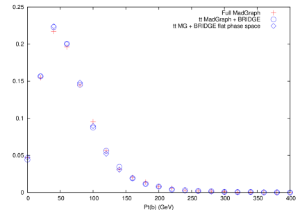
Figure 1: We have generated $t\bar{t}$ events in MadGraph and decayed them with BRIDGE, and also generated $e^{+}\nu_{e}be^{-}\bar{\nu}_{e}\bar{b}$ events in MadGraph. Here we plot the $p_{T}$ histogram for the $b$ quark in the decayed events versus the full matrix element. In this and other figures, the histograms are normalized to have the same area. In this figure we also show $t\bar{t}$ events from MadGraph decayed with BRIDGE with the amplitude set to 1, so that the decay is governed by the phase space volume.

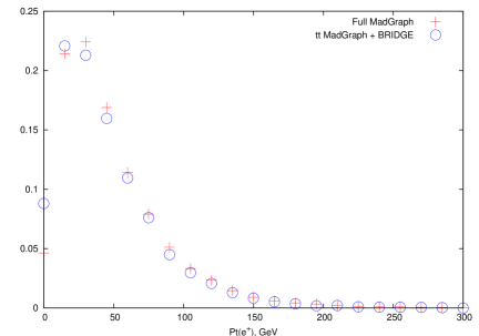
Figure 2: The $p_{T}$ histogram for the $e^{+}$ in the decayed events versus the full matrix element.

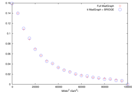
Figure 3: The $M^{2}(b\bar{b})$ histogram in the decayed events versus the full matrix element.

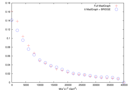
Figure 4: The $M^{2}(e^{+}e^{-})$ histogram in the decayed events versus the full matrix element.

As a first test of DGE, we present transverse momentum distributions for the decay chain $t\rightarrow W^{+}b\rightarrow e^{+}\nu_{e}b$, where the tops are chosen from $t\bar{t}$ events. We generated $t\bar{t}$ events with MadGraph and decayed them in BRIDGE, and also generated a set of $e^{+}\nu_{e}be^{-}\bar{\nu}_{e}\bar{b}$ events directly in MadGraph (demanding that the relevant diagrams contain a $t\bar{t}$). The $p_{T}$ distribution for the $b$ quark is shown in Figure 1, and for the $e^{+}$ in Figure 2. The distributions agree reasonably well. For the $p_{T}$ of the $b$ we also show the distribution computed with a flat phase space approximation for the decay (i.e., we set the amplitude to $1$ independent of the momenta). In this case, the flat phase space agrees quite well. We will see a later example for which the structure of the amplitude is important, and is captured by BRIDGE, but a flat phase space amplitude is a poor approximation.

Next, we plot a more complicated quantity that involves information from both sides of the event: the invariant mass squared $M^{2}_{b\bar{b}}$, in Figure 3, and $M^{2}_{e^{+}e^{-}}$ in Figure 4. There is a discrepancy in $M^{2}_{e^{+}e^{-}}$, where BRIDGE seems to underestimate the number of events with a very low invariant mass for the $e^{+}e^{-}$ pair. Because invariant masses involve not only the momenta but the angular distance between the particles, this suggests that there might be some errors in angular distributions that involve correlations between opposite sides of an event. Still, the discrepancy is not huge (BRIDGE is about 13% low for the first bin).

Angular correlations can carry information about the helicity structure of various couplings. We’ll now turn to a specific example and show that BRIDGE clearly distinguishes left- and right-handed chiral gauge couplings.

3.2 $W$ Polarization In Top Decays

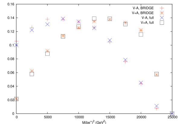
Figure 5: Histogram of $M_{e^{+}b}$ computed from MadGraph $t\bar{t}$ events decayed with BRIDGE compared to MadGraph $e^{+}\nu_{e}b\bar{t}$ events. In both cases the $V-A$ and $V+A$ structures for the $W^{+}\bar{t}b$ vertex are compared.

Let’s consider a simple example that illustrates the success of BRIDGE in reproducing the proper helicity structure of decays: in decays of the top quark, $t\rightarrow W^{+}b$, we expect 70% of the $W$ bosons to be longitudinally polarized, 30% to be left-circularly polarized, and very few to be right-circularly polarized. (The fraction of longitudinally polarized $W$s can be computed as $\frac{x}{x+2}$ where $x=\frac{m_{t}^{2}}{m_{W}^{2}}\approx 4.7$.)

$W$ polarization is experimentally studied as a probe of the $V-A$ structure of the $tWb$ vertex. In this case one examines the decay chain $t\rightarrow W^{+}b\rightarrow\ell^{+}\nu_{\ell}b$, where $\ell=e,\mu$. The invariant mass $M_{\ell b}$ is then sensitive to the angular structure of the decay. This has been studied experimentally by the CDF Collaboration [16].

As a test of BRIDGE, we have simulated $t\bar{t}$ events with MadGraph and then used DGE to decay $t\rightarrow W^{+}b$, $W^{+}\rightarrow e^{+}\nu_{e}$. We have then produced a separate set of decayed events for which we have altered the structure of the $tWb$ vertex to be $V+A$. In each case we have plotted the invariant mass $M_{e^{+}b}$. We have produced the same plots with a MadGraph simulation of production of $e^{+}\nu_{e}b\bar{t}$ (requiring the $e^{+}\nu_{e}b$ to come from a top), which will maintain the full angular correlations. The results are compared in Figure 5. The output of DGE is rather close to the full MadGraph answer, and clearly shows the distinction between $V-A$ and $V+A$.

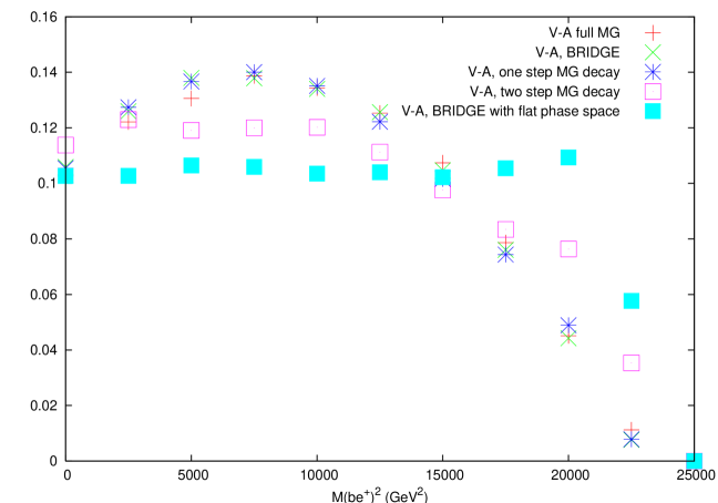
Figure 6: Histogram of $M_{e^{+}b}$ computed from MadGraph $t\bar{t}$ events decayed with BRIDGE compared to the same events decayed with MadGraph’s “decay” program in two steps ($t\rightarrow W^{+}b$, $W^{+}\rightarrow e^{+}\nu_{e}$) or in one step, and to full MadGraph $e^{+}\nu_{e}b\bar{t}$ events. The final curve is BRIDGE with the amplitude simply replaced by $1$, to obtain a distribution depending only on phase space volume. Only the $V-A$ structure for the $W^{+}\bar{t}b$ vertex is shown.

As a comparison, we show in Figure 6 the same two curves for the $V-A$ structure only, as well as three additional curves. The third curve comes from using the MadGraph decay code to decay the same simulated $t\bar{t}$ events that we decayed with DGE, using two sequential decay steps ($t\rightarrow W^{+}b$ followed by $W^{+}\rightarrow e^{+}\nu_{e}$). The fourth curve uses the MadGraph decay code to decay the same events, in only one step ($t\rightarrow e^{+}\nu_{e}b$). For the one-step decay, MadGraph builds the full amplitude and does a three-body phase space integral instead of doing two successive decays. The final curve shows the decay done in DGE but with the amplitude replaced by a constant, so that the decay depends only on phase space volume. From the figure, it is apparent that DGE and the one-step MadGraph decay both model the full MadGraph result accurately, whereas the two-step MadGraph decay is less accurate. The two-step MadGraph decay is still significantly more accurate than a naive flat phase space decay, however. DGE and the two-step MadGraph decay are performing nearly identical operations, but DGE is doing both decay steps in the rest frame of the top. On the other hand, MadGraph is doing decays in the center-of-mass frame of the collision. As a result, in the frame MadGraph works in, many of the $W^{+}$ bosons will be right-handed, and some of the information about the angular structure is lost. The choice of frame that we make in DGE allows for a more accurate result. (To see this, one can generate $t\bar{t}$ events just above threshold in MadGraph. On these events, the MadGraph two-step decay curve matches the others quite well.) As we mentioned in Section 2.2.1, we do not yet know precisely under what conditions DGE gives reliable angular distributions and in what conditions it loses important correlations. It would be very interesting to study this further. For now, this example shows that DGE can accurately reproduce some nontrivial angular effects. We will see another example in Section 3.3.

3.3 MSSM

We briefly here discuss how the MSSM is designed to be used with BRIDGE. We provide two executables runBRIsusy.exe and runDGEsusy.exe that are specifically designed for the MSSM. We note however that this in no way means it is necessary to generate new versions of the BRI and DGE executables for a generic model. As discussed in Section 2 any new model implemented in the framework of the Madgraph usrmod can be accommodated regardless of complexity. However, since the MSSM is well defined in its couplings and there exists a standard SLHA interface to spectrum calculators runBRIsusy.exe and runDGEsusy.exe were designed to specifically work with this format. In the future the SUSY versions of runDGE and runBRI may be reincorporated into the non-SUSY runDGE and runBRI, but for now we will explain the existing interface.

As alluded to, the only main difference between the SUSY and non-SUSY versions of BRIDGE is the input format. As discussed in Section 2 the model is defined by four files, particles.dat, interactions.dat, couplings_check.txt, and param_card.dat. The use of the couplings and param card files are what defines the numerical values of the masses and couplings in a generic usrmod file. However, in the context of the MSSM there is a specific format for defining the model parameters [10] and the couplings of the model are well defined. For this reason instead of having the user only interface couplings through their numerical values as in the usrmod version of input, the couplings are defined separately in a file SUSYpara.cpp and read directly from param_card.dat through the SLHA read routines in SLHArw.cpp. The coupling definitions found in SUSYpara.cpp are based upon those written originally for the SMadgraph project [17], that have since been incorporated into Madgraph v4. If one wanted to modify the format of the MSSM couplings beyond the original assumptions implemented in Smadgraph, the files SUSYpara.cpp and SLHArw.cpp are all that are necessary to be modified.

The actual parameters used from the SLHA formatted input file are those found in the blocks corresponding to mixing matrices for the various supersymmetric particles, masses, SM inputs, A terms, Yukawa couplings and Higgs parameters. Additionally if available BLOCK GAUGE is used to define the SM gauge couplings evolved to the scale specified by the spectrum calculator. BRIDGE does not run the SM couplings so BLOCK GAUGE is used to define couplings at a higher scale if available, if not the default values at $m_{Z}$ are used.

The output of runBRIsusy.exe is in the form of SLHA formatted decay tables. These decay tables can be then used with any program that can handle SLHA formatted input. runDGEsusy.exe is used in the same way as runDGE.exe. Given the common definition of the MSSM, DGE can also be used to decay Les Houches formatted event files created by other matrix element generators for the MSSM..

3.3.1 SLHA Decay Table Comparison

In this section we demonstrate the numerical accuracy of using BRI with the MSSM. We will compare BRI against the well tested SUSY-HIT program[13], which is the continuation of the SDECAY program[12] combined with HDECAY[11]. We will for simplicity(lack of imagination) use the point SPS-1a, the SLHA formatted spectrum card can be downloaded from the SUSY-HIT webpage. There are a few factors that influence the results of this comparison. First SUSY-HIT includes the effects of loops on decays, whereas by default BRIDGE does not. Therefore certain decays for which SUSY-HIT includes loop corrections would be expected to differ slightly. Additionally decays that do not exist in the MSSM at tree level are included in SUSY-HIT and would have to be added separately into BRIDGE as will be discussed in Section 3.4. Additionally any effects from running of the couplings that are included in SUSY-HIT beyond the definition of the couplings at the given scale in BLOCK GAUGE will be unaccounted for in BRIDGE. Given that the full SLHA decay tables for the MSSM would add many pages to this manual we will only present as an example the decay tables for $\chi_{2}^{+}$ and $\tilde{d}_{L}$ in Tables 1 and 2.

	BRI	SUSY-HIT
$\chi_{2}^{+}$ Decays	$\Gamma_{\mathrm{BRI}}=$2.57908720E+00	$\Gamma_{\mathrm{SUSY-HIT}}=$2.51618431E+00
BR($\chi_{2}^{+}$ $\rightarrow$ $\chi_{1}^{+}$ Z )	2.36511304E-01	2.40213561E-01
BR($\chi_{2}^{+}$ $\rightarrow$ $\chi_{1}^{0}$ $W^{+}$ )	6.55162205E-02	6.48085350E-02
BR($\chi_{2}^{+}$ $\rightarrow$ $\chi_{2}^{0}$ $W^{+}$ )	2.83642506E-01	2.86434649E-01
BR($\chi_{2}^{+}$ $\rightarrow$ $\chi_{1}^{+}$ h )	1.66651066E-01	1.70182080E-01
BR($\chi_{2}^{+}$ $\rightarrow$ $\nu_{e}\tilde{e}^{+}$ )	5.35091797E-02	5.44450726E-02
BR($\chi_{2}^{+}$ $\rightarrow$ $e^{+}\tilde{\nu}_{e}$ )	2.07052458E-02	2.10374477E-02
BR($\chi_{2}^{+}$ $\rightarrow$ $\nu_{\mu}\tilde{\mu}^{+}$ )	5.32258593E-02	5.44450726E-02
BR($\chi_{2}^{+}$ $\rightarrow$ $\mu^{+}\tilde{\nu}_{\mu}$ )	2.07805107E-02	2.10374477E-02
BR($\chi_{2}^{+}$ $\rightarrow$ $\nu_{\tau}\tilde{\tau}_{1}^{+}$ )	2.64808582E-03	1.86804725E-04
BR($\chi_{2}^{+}$ $\rightarrow$ $\nu_{\tau}\tilde{\tau}_{2}^{+}$ )	6.24909217E-02	5.89508529E-02
BR($\chi_{2}^{+}$ $\rightarrow$ $\tau^{+}\tilde{\nu}_{\tau}$ )	3.43191004E-02	2.82584766E-02

Table 1: $\chi_{2}^{+}$ decays in the MSSM for SPS-1a, calculated in both BRIDGE and SUSY-HIT. The decay widths listed are in GeV.

	BRI	SUSY-HIT
$\tilde{d}_{L}$ Decays	$\Gamma_{\mathrm{BRI}}=$5.25084508E+00	$\Gamma_{\mathrm{SUSY-HIT}}=$5.25959716E+00
BR($\tilde{d}_{L}$ $\rightarrow$ d $\chi_{1}^{0}$ )	2.37791027E-02	2.37748353E-02
BR($\tilde{d}_{L}$ $\rightarrow$ d $\chi_{2}^{0}$ )	3.09521294E-01	3.05370011E-01
BR($\tilde{d}_{L}$ $\rightarrow$ d $\chi_{3}^{0}$ )	1.67844811E-03	1.79694702E-03
BR($\tilde{d}_{L}$ $\rightarrow$ d $\chi_{4}^{0}$ )	1.68190300E-02	1.80395085E-02
BR($\tilde{d}_{L}$ $\rightarrow$ u $\chi_{2}^{-}$ )	6.01085498E-01	6.00388839E-01
BR($\tilde{d}_{L}$ $\rightarrow$ u $\chi_{2}^{-}$ )	4.71166268E-02	5.06298586E-02

Table 2: $\tilde{d}_{L}$ decays in the MSSM for SPS-1a, calculated in both BRIDGE and SUSY-HIT. The decay widths listed are in GeV.

The results of the comparison between BRI and SUSY-HIT are very good. For the decays listed in Tables 1 and 2 the differences between BRIDGE and SUSY-HIT are on the percent level or less. Examining some of the decays where loop corrections are important the agreement stays on the order of 5% difference at most. We have only compared particle decay tables for particles that have two body decays only, or just the partial widths for those particles which have both two and three body decays.

3.3.2 Slepton Spin Correlations Example

As another check of the DGE program, specifically the executable runDGEsusy.exe, we can examine how well it keeps possible spin correlations. As an example of spin correlation we will look at the example studied in [18], in which the process

$$pp>\tilde{l}^{+}\tilde{l}^{-}>l^{+}l^{-}\chi^{0}_{1}\chi^{0}_{1}$$ (3.1)

was studied. It was shown in [18] that by studying the variable

$$\cos\theta^{*}_{ll}\equiv\tanh^{-1}\left(\frac{\Delta\eta_{ll}}{2}\right)$$ (3.2)

where $ll$ refers to the outgoing $l^{+}$ $l^{-}$ pair, that this variable encodes the spin correlation of the sleptons that were originally produced. Since this spin correlation variable, which is similar to the variables $\eta_{+}$ and $\eta_{-}$ studied in [19], takes into account opposite sides of the diagram it is not obvious that decaying the particles separately, as in DGE, will capture most of the spin dependent effects.

Figure 7: Normalized histogram of $\cos\theta^{*}_{ll}$ computed from MadGraph $\tilde{l}\tilde{l}$ events decayed with BRIDGE compared to MadGraph $l^{+}l^{-}\chi^{0}_{1}\chi^{0}_{1}$ events.

In Figure 7 we plot $\cos\theta^{*}_{ll}$ for SPS-1a from the full matrix element calculation in Madgraph and compare to the results of first generating $pp>\tilde{l}^{+}\tilde{l}^{-}$ in Madgraph and then decaying the sleptons using DGE. What we find is that DGE seems to keep a remarkable amount of spin correlation as compared to just generating a flat matrix element, which for comparison was done in [18]. Of course this is only a one step decay chain but nevertheless the results are very encouraging. It would be very interesting as future work to quantify more fully the amount of spin correlation that DGE captures in more complicated decay chains. In particular studying some of the examples/variables suggested for spin correlations in the MSSM suggested in [19, 20] would serve as a good starting point.

3.3.3 SPS2

$\tilde{g}$ Decays	BRIDGE $\Gamma$(GeV)	SUSY-HIT $\Gamma$(GeV)
$\tilde{g}\rightarrow d\bar{d}\chi_{1}^{0}$	2.156 $\times 10^{-5}$	3.486 $\times 10^{-5}$
$\tilde{g}\rightarrow d\bar{d}\chi_{2}^{0}$	0.867 $\times 10^{-4}$	1.136 $\times 10^{-4}$
$\tilde{g}\rightarrow d\bar{d}\chi_{3}^{0}$	2.356 $\times 10^{-7}$	1.480 $\times 10^{-7}$
$\tilde{g}\rightarrow d\bar{d}\chi_{4}^{0}$	3.365 $\times 10^{-6}$	5.179 $\times 10^{-6}$
$\tilde{g}\rightarrow d\bar{u}\chi_{1}^{+}$	1.781 $\times 10^{-4}$	2.369 $\times 10^{-4}$
$\tilde{g}\rightarrow d\bar{u}\chi_{2}^{+}$	6.643 $\times 10^{-6}$	9.377 $\times 10^{-6}$

Table 3: Some of the $\tilde{g}$ decays in the MSSM for SPS-2, calculated in both BRIDGE and SUSY-HIT. The decay widths listed are in GeV.

The SPS2 spectrum has squarks heavier than the gluino, so it gives a useful check of 3-body decay widths. We do not expect extremely close agreement with SUSY-HIT, as it includes loop effects. We present a comparison in Table 3. It is reassuring that the widths are relatively close. (The three-body code accurately computes the muon decay width, so it seems reasonable to expect that the differences here are due to the loops.)

3.3.4 Gluino distributions

As a further check of the 3-body code, we implemented a toy model with a gluino at 1 TeV, one squark at 1.025 TeV, and a neutralino at 100 GeV. We then simulated gluino production and decay with $\tilde{g}\rightarrow q\bar{q}\tilde{\chi}_{0}^{1}$, both fully in MadGraph and MadGraph $\tilde{g}\tilde{g}$ production with gluinos decayed by BRIDGE. We plot the resulting distributions in Figures 8 and 9.

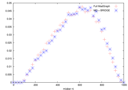
Figure 8: Normalized histogram of $m(\bar{q}\tilde{\chi}_{0}^{1})$ computed from MadGraph $\tilde{g}\tilde{g}$ events decayed with BRIDGE compared to MadGraph $\tilde{g}q\bar{q}\tilde{\chi}_{0}^{1}$ events.

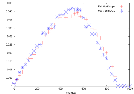
Figure 9: Normalized histogram of $m(\bar{q}q)$ computed from MadGraph $\tilde{g}\tilde{g}$ events decayed with BRIDGE compared to MadGraph $\tilde{g}q\bar{q}\tilde{\chi}_{0}^{1}$ events.

3.4 Loop example: a user-defined vertex for $h\rightarrow gg$

If one uses the standard HELAS amplitudes, one will necessarily miss decays that happen only at loop level. In the Standard Model these decays are potentially important; for instance, we might want to consider $h\rightarrow gg$ or $h\rightarrow\gamma\gamma$. We have provided an example of how to incorporate such decays in BRIDGE; if one has already implemented such a vertex for MadGraph, it requires minimal effort to adapt it for BRIDGE. One implementation of such couplings is present in the heft model included in MadGraph. Here we discuss an alternative approach, directly implementing the loop diagram.

First, one must implement the desired vertex as a new HELAS routine. We provide an example, vvsjxx.F, for the Higgs–glue–glue vertex in the Standard Model (we consider only the top loop contribution). To calculate the correct momentum dependence of the vertex one can use a library like FF or LoopTools to evaluate integrals [21]. You will have to be sure to link your new routine in the HELAS library (or add it to the makefile for BRIDGE). Next, as in MadGraph, one should add an additional character J at the end of the relevant line of interactions.dat for the vertex. This character is stored by the relevant Vertex object of BRIDGE, and then passed to the corresponding amplitude function (in this case, VVSAmp) as a variable called usrFlag. Now, the code in Amplitude.cpp has lines set off by #ifdef USE_VVSJXX and #endif. If this preprocessor flag is set, the code declares the new Fortran routine vvsjxx_, which is called if the special character J is passed from the amplitude. More HELAS routines can always be added in this manner; the only part of the BRIDGE code that should need modification to deal with them is Amplitude.cpp, so long as they involve only scalars, vectors, and spin one-half fermions. (Note that yet another option is to directly code the one-loop amplitudes in C++, if one is not also planning to use the new HELAS routine with MadGraph or some other program.)

For the width $h\rightarrow gg$, we expect at one loop:

$$\Gamma(h\rightarrow gg)=\frac{\alpha m_{h}}{8\sin^{2}\theta_{W}}\left(\frac{m_{h}}{m_{W}}\right)^{2}\left(\frac{\alpha_{s}}{3\pi}\right)^{2}\left|I\left(\frac{m_{t}}{m_{h}}\right)\right|^{2},$$ (3.3)

where $I(x)$ is an order-one quantity that can be expressed as an integral over a Feynman parameter. We compare the numerical result of the one-loop calculation to the output of BRIDGE for the same quantity in Table 4. The BRIDGE numbers agree within about 2%.

Higgs Mass	$\Gamma(h\rightarrow gg)$, 1-loop	$\Gamma(h\rightarrow gg)$, BRIDGE
60	$2.55\times 10^{-5}$	$2.51\times 10^{-5}$
120	$2.13\times 10^{-4}$	$2.09\times 10^{-4}$
180	$7.77\times 10^{-4}$	$7.64\times 10^{-4}$
240	$2.08\times 10^{-3}$	$2.05\times 10^{-3}$
300	$4.99\times 10^{-3}$	$4.88\times 10^{-3}$

Table 4: Higgs partial widths to two gluons, one-loop calculation versus BRIDGE result with one-loop HELAS vertex added. All numbers are in GeV.

4 Conclusions and Future Development

BRIDGE can speed up the process of simulating a new model, when used with other tools like MadGraph. It also provides a quick tree-level calculator for decay rates, which can be a useful start for understanding the phenomenology of a model. Furthermore, we have seen that BRIDGE accurately models certain nontrivial angular effects. One remaining issue is to consider finite (but narrow) width effects: currently intermediate particles in a long decay chain will be exactly on shell, whereas we would like to have a Breit-Wigner distribution (while keeping as much angular information as possible).

In addition, we plan to continue working with the MadGraph authors to ensure that BRIDGE will interact smoothly with their code. It should also be possible to use BRIDGE independently of MadGraph, provided you have the HELAS libraries. BRIDGE could be applied to a wider array of models if new HELAS routines are developed (e.g., for particles of spin greater than 1), so this is another direction in which further work could be useful. The potential usefulness of BRIDGE and other intermediate programs for studying beyond the SM physics also suggests the need for a standard definition of a new physics model akin to what we have used in the Madgraph model definitions. One final direction to consider involves the variable SPINUP in the Les Houches format. We have seen that we obtain reasonably accurate angular distributions by using the helicity in the same frame for every decay along a chain; we store this helicity in the SPINUP column. As with any choice of a single number to characterize spin, this is losing some information. Given the degree of interest in spin effects in the collider phenomenology community, perhaps we should consider expanding the Les Houches format to allow a more sophisticated presentation of spin information?

The code for BRIDGE is distributed at http://lepp.cornell.edu/public/theory/BRIDGE/. We encourage you to report bugs or (even better) fix them or contribute new features. If you use BRIDGE in a publication we request that you cite this document. An up-to-date version of this manual will be maintained on the BRIDGE website.

References

- [1] T. Sjostrand, S. Mrenna and P. Skands, JHEP 0605, 026 (2006) [arXiv:hep-ph/0603175].
- [2] G. Corcella et al., JHEP 0101, 010 (2001) [arXiv:hep-ph/0011363]; G. Corcella et al., arXiv:hep-ph/0210213.
- [3] A. Pukhov et al., Phys. Rev. D 66, 010001 (2002) arXiv:hep-ph/9908288; E. Boos et al. [CompHEP Collaboration], Nucl. Instrum. Meth. A 534, 250 (2004) [arXiv:hep-ph/0403113].
- [4] A. Pukhov, arXiv:hep-ph/0412191.
- [5] T. Stelzer and W. F. Long, Comput. Phys. Commun. 81, 357 (1994) [arXiv:hep-ph/9401258]; F. Maltoni and T. Stelzer, JHEP 0302, 027 (2003) [arXiv:hep-ph/0208156].
- [6] B. P. Kersevan and E. Richter-Was, Comput. Phys. Commun. 149, 142 (2003) [arXiv:hep-ph/0201302].
- [7] F. Krauss, R. Kuhn and G. Soff, JHEP 0202, 044 (2002) [arXiv:hep-ph/0109036].
- [8] T. Ishikawa, T. Kaneko, K. Kato, S. Kawabata, Y. Shimizu and H. Tanaka [MINAMI-TATEYA group], “GRACE manual: Automatic generation of tree amplitudes in Standard Models: Version 1.0.”
- [9] E. Boos et al., arXiv:hep-ph/0109068; J. Alwall et al., Comput. Phys. Commun. 176, 300 (2007) [arXiv:hep-ph/0609017].
- [10] P. Skands et al., JHEP 0407, 036 (2004) [arXiv:hep-ph/0311123].
- [11] A. Djouadi, J. Kalinowski and M. Spira, Comput. Phys. Commun. 108, 56 (1998) [arXiv:hep-ph/9704448].
- [12] M. Muhlleitner, A. Djouadi and Y. Mambrini, Comput. Phys. Commun. 168, 46 (2005) [arXiv:hep-ph/0311167].
- [13] A. Djouadi, M. M. Muhlleitner and M. Spira, arXiv:hep-ph/0609292.
- [14] G. P. Lepage, J. Comput. Phys. 27, 192 (1978), G. P. Lepage, CLNS-80/447
- [15] H. Murayama, I. Watanabe and K. Hagiwara, KEK-91-11 (1992).
- [16] D. Acosta et al. [CDF Collaboration], Phys. Rev. D 71, 031101 (2005) [Erratum-ibid. D 71, 059901 (2005)] [arXiv:hep-ex/0411070], A. Abulencia et al. [CDF Collaboration], arXiv:hep-ex/0608062.
- [17] G. C. Cho, K. Hagiwara, J. Kanzaki, T. Plehn, D. Rainwater and T. Stelzer, Phys. Rev. D 73, 054002 (2006) [arXiv:hep-ph/0601063].
- [18] A. J. Barr, JHEP 0602, 042 (2006) [arXiv:hep-ph/0511115].
- [19] P. Meade and M. Reece, Phys. Rev. D 74, 015010 (2006) [arXiv:hep-ph/0601124].
- [20] A. J. Barr, Phys. Lett. B 596, 205 (2004) [arXiv:hep-ph/0405052]; J. M. Smillie and B. R. Webber, JHEP 0510, 069 (2005) [arXiv:hep-ph/0507170]; A. Alves, O. Eboli and T. Plehn, Phys. Rev. D 74, 095010 (2006) [arXiv:hep-ph/0605067]; L. T. Wang and I. Yavin, arXiv:hep-ph/0605296; J. M. Smillie, arXiv:hep-ph/0609296.
- [21] G. J. van Oldenborgh, Comput. Phys. Commun. 66, 1 (1991); T. Hahn, Nucl. Phys. Proc. Suppl. 89, 231 (2000) [arXiv:hep-ph/0005029].