Constraints on flavor-changing neutral-current couplings from the signal of associated production with QCD next-to-leading order accuracy at the LHC
Abstract
We study a generic Higgs boson and a top quark associated production via model-independent flavor-changing neutral-current couplings at the LHC, including complete QCD next-to-leading order (NLO) corrections to the production and decay of the top quark and the Higgs boson. We find that QCD NLO corrections can increase the total production cross sections by about 48.9% and 57.9% for the and coupling induced processes at the LHC, respectively. After kinematic cuts are imposed on the decay products of the top quark and the Higgs boson, the QCD NLO corrections are reduced to for the coupling induced process and almost vanish for the coupling induced process. Moreover, QCD NLO corrections reduce the dependence of the total cross sections on the renormalization and factorization scales. We also discuss signals of the associated production with the decay mode and production with the decay mode . Our results show that, in some parameter regions, the LHC may observe the above signals at the level. Otherwise, the upper limits on the FCNC couplings can be set.
pacs:
14.65.Ha, 12.38.Bx, 12.60.FrI INTRODUCTION
Recently the ATLAS and CMS collaborations at the Large Hadron Collider (LHC) have discovered a new particle with a mass of about 125 GeV Chatrchyan et al. (2012); Aad et al. (2012). In the near future, the most important task is to study the intrinsic properties of this new particle, such as the couplings and spin, which will determine whether it is the Standard Model (SM) Higgs boson, and lead to deeper understanding of electroweak (EW) symmetry breaking mechanism.
It is attractive to investigate the anomalous couplings of a generic Higgs boson, such as the anomalous couplings with quarks via flavor-changing neutral-current (FCNC). In the SM, FCNC is absent at tree level, and is suppressed at one-loop level by the Glashow-Iliopoulos-Maiani mechanism Glashow et al. (1970). The anomalous couplings, if exist, are strong evidence of New Physics (NP). In Ref. Blankenburg et al. (2012), indirect constraints on FCNC couplings from low-energy experiments are studied and used to analyze the process of the Higgs boson decaying to light quarks or leptons. But the FCNC couplings between the Higgs boson and the top quark are not discussed there.
The top quark mass is close to the EW symmetry breaking scale. Thus it is an appropriate probe for the EW symmetry breaking mechanism and NP. Any deviation from SM prediction for precise observables involving top quarks exhibits hints of NP. The production of a single top quark associated with a gluon jet or a vector boson via FCNC couplings has already been investigated at the leading order (LO) Aguilar-Saavedra (2004); del Aguila et al. (1999); Aguilar-Saavedra (2001); Aguilar-Saavedra and Branco (2000) and at the next-to-leading order (NLO) Liu et al. (2005); Zhang et al. (2009); Gao et al. (2009); Zhang et al. (2011); Li et al. (2011), respectively. In this paper, we will discuss the constraints on the FCNC couplings from the signal of the Higgs boson and the top quark associated production with QCD NLO accuracy at the LHC.
In some NP models, the FCNC couplings of the Higgs boson and the top quark can be generated at tree level, or enhanced to observable levels through radiative corrections Aguilar-Saavedra (2004); Yang (2005); del Aguila et al. (1999); Aguilar-Saavedra (2001); Aguilar-Saavedra and Branco (2000); Liu et al. (2005); Zhang et al. (2009); Gao et al. (2009); Zhang et al. (2011); Li et al. (2011), such as the two Higgs doublet models III Bejar et al. (2003); Cao et al. (2005a), the minimal supersymmetric models (MSSM) Guasch and Sola (1999); Bejar et al. (2001); Yang and Li (1994); de Divitiis et al. (1997); Diaz-Cruz et al. (2002); Cao et al. (2006), the topcolor-assisted technicolor model Cao et al. (2005a), the exotic quarks models and the left-right symmetric models Gaitan et al. (2006); Arhrib and Hou (2006). Since we do not know which type of NP will be responsible for the future deviation, it is better to study the FCNC processes with a model independent method. In general, the interactions between the Higgs boson, the top quark and a light quark can be expressed as Aguilar-Saavedra (2004)
| (1) |
where defining the strength of the coupling is a real coefficient, while , are complex numbers, normalized to . The constraints on the above couplings have been set through indirect low-energy processes in Refs. Fernandez et al. (2010); Aranda et al. (2010); Larios et al. (2005). It is interesting to study how to set the direct constraints on the above couplings from the signals of the top quark and the Higgs boson associated production and top pair production with top quark rare decay at the hadron colliders. These processes have been studied at the LO in Ref. Aguilar-Saavedra (2004). However, the LO total cross sections at the hadron collider suffer from large uncertainties due to the arbitrary choices of the renormalization and factorization scales. Besides, at the NLO level the additional radiation makes jets, which are the products of the Higgs boson and the top quark, softer and the mass distribution of the reconstructed particles broader, which will affect events selection when kinematic cuts are imposed. Thus, it is necessary to perform complete QCD NLO calculations of these processes at the LHC, including production and decay.
The process , which has the similar scattering amplitude to the process we study in this paper, has been discussed in the two Higgs double models and supersymmetry, including the QCD NLO or supersymmetry QCD corrections Plehn (2003); Weydert et al. (2010); Zhu (2003); Klasen et al. (2012). After considering the difference from the couplings and parton distribution functions (PDFs), our numerical results for the production are consistent with the their results in the range of Monte Carlo integration error. However, in the process we study, the Higgs boson is neutral and has a mass around 125 GeV, usually much less than the mass of charged Higgs boson, which leads to significantly different decay modes and signals at the hadron colliders.
The arrangement of this paper is as follows. In Sec. II, we present the LO results for the Higgs boson and the top quark associated production induced by FCNC couplings. In Sec. III, we describe the detailed calculations of the NLO results, including the virtual and real corrections. Then in Sec. IV, we investigate numerical results, in which we discuss the scale uncertainties and give some important kinematic distributions. In Sec.V, we discuss the signals of associated production with the decay mode and , and production with rare decay mode . Then we analysis the discovery potential with QCD NLO accuracy at the LHC with TeV. Section VI is a brief conclusion.
II LEADING ORDER RESULTS
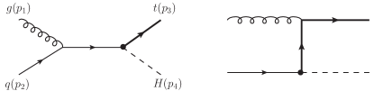
At the hadron colliders, there is only one subprocess that contributes to the associated production at the LO via FCNC couplings:
| (2) |
where is either or quark. The Feynman diagrams are shown in Fig. 1.
After summing (averaging) over the spins and colors of the final-(initial-)state particles, the explicit expression of the squared amplitude at the LO is
| (3) | |||||
where and are the top quark mass and the Higgs boson mass, respectively. The Mandelstam variables , , and are defined as
| (4) |
The LO total cross section at hadron colliders is given by convoluting the partonic cross section with the PDFs in the proton,
| (5) |
where is the factorization scale, and is Born level partonic cross section.
III THE NEXT-TO-LEADING ORDER CALCULATIONS
In this section, we present QCD NLO corrections of associated production using dimensional regularization scheme with naive prescription in dimensions to regularize the ultraviolet (UV) and infrared (IR) divergences. The NLO corrections contain the virtual gluons effects and the real radiation of a gluon or a massless quark. The corresponding Feynman diagrams are shown in Fig. 2 and 3, respectively. We use two cutoff phase space slicing method Harris and Owens (2002) in the real corrections to separate the IR divergences.
III.1 Virtual corrections
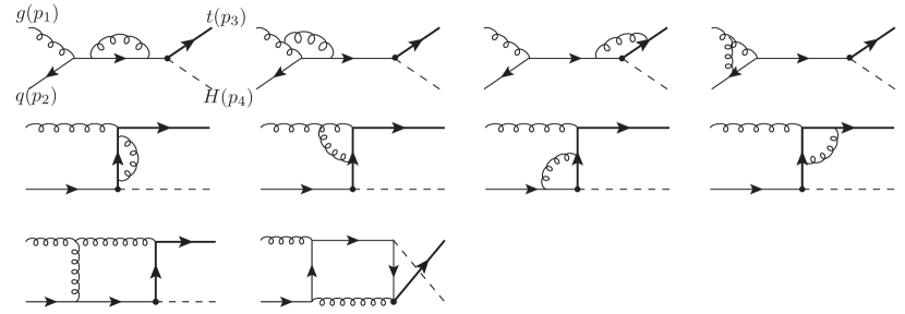
The virtual corrections come from the interference of the one-loop amplitude with the Born amplitude:
| (6) |
We introduce counterterms to absorb UV divergences. For the external fields, we fix all the renormalization constants using the on shell renormalization scheme:
| (7) |
where , is the renormalization scale and . For the counterterm of FCNC couplings , we use the modified minimal subtraction () scheme Zhang et al. (2010):
| (8) |
and the running of the FCNC coupling is given by
| (9) |
Here is the one-loop coefficients of the QCD -function.
In the virtual corrections, the UV divergences are canceled by the counterterms. To deal with IR divergences, we adopt the traditional Passarino-Veltman reduction method to reduce the tensor integrals to scalar integrals Passarino and Veltman (1979); Denner (1993), of which the IR divergences can be obtained by the skill in Ref. Ellis and Zanderighi (2008). And the IR divergent parts are given by
| (10) |
where
| (11) |
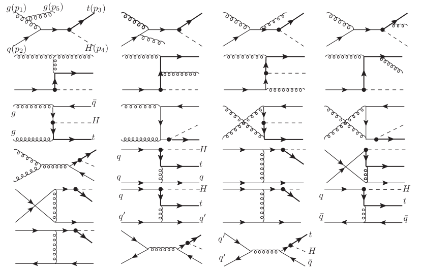
III.2 Real corrections
The real corrections contain the radiations of an additional gluon, and massless (anti)quark. The relevant Feynman diagrams are shown in Fig. 3.
The partonic cross section can be written as
| (12) |
We use two cutoff phase space slicing method Harris and Owens (2002), which introduces two small cutoffs and to divide the three-body phase space into three regions. First, the phase space is separated into two regions according to whether or not the energy of the additional gluon satisfies the soft criterion in the partonic center-of-mass frame (CMF). And the partonic cross section can be divided as
| (13) |
where and are the contributions from the hard and the soft regions, respectively. Furthermore, the collinear cutoff is applied to separate the hard region into two regions according to whether the collinear condition is satisfied or not, where with . The corresponding cross section is splited into
| (14) |
where the contributions from hard-collinear regions contain the collinear divergences, and the hard-noncollinear part is free of IR singularities and can be calculated numerically.
III.2.1 Real gluon emission
In the limit that the energy of the emitted gluon becomes small, i.e., , the amplitude squared can be factorized into the Born amplitude squared and the eikonal factor :
| (15) |
where the eikonal factor can be expressed as
| (16) | |||||
with . The three-body phase space in the soft region can be factorized into
| (17) |
where is the integration over the phase space of the soft gluon, given by
| (18) |
Hence, the parton level cross section in the soft region can be expressed as
| (19) |
After integration over the soft phase space, Eq. (19) becomes
| (20) |
with
| (21) |
The are defined as
| (22) |
where and .
In the hard-collinear region, collinear singularities arise when the emitted hard gluon is collinear to the incoming massless partons. As the conclusion of the factorization theorem Collins et al. (1985); Bodwin (1985), the amplitude squared can be factorized into the product of the Born amplitude squared and the Altarelli-Parisi splitting function; that is
| (23) |
where denotes the fraction of the momentum of the incoming parton carried by . The unregulated Altarelli-Parisi splitting functions are written explicitly as Harris and Owens (2002)
| (24) |
Then we factorize the three-body phase space in the collinear limit as
| (25) |
Thus, after convoluting with the PDFs, the three-body cross section in the hard-collinear region can be written as Harris and Owens (2002)
| (26) | |||||
where is the bare PDF.
III.2.2 Massless (anti)quark emission
In addition to the real gluon emission, an additional massless in the final state should be taken into consideration at of the perturbative expansion. Since the contributions from real massless emission contain initial-state collinear singularities, we need to use the two cutoff phase space slicing method Harris and Owens (2002) to isolate these collinear divergences. The cross section for the process with an additional massless emission, including the noncollinear part and collinear part, can be expressed as
| (27) | |||||
where
| (28) |
The is the noncollinear cross sections for the processes of the , and initial states:
| (29) | |||||
in which is the three-body phase space in the noncollinear region.
III.2.3 Mass factorization
There are still collinear divergences in the partonic cross sections after adding the renormalized virtual corrections and the real corrections. The remaining divergences can be factorized into a redefinition of the PDFs. In the convention the scale-dependent PDF can be written as Harris and Owens (2002)
| (30) | |||||
The Altarelli-Parisi splitting function is defined by
| (31) |
The resulting expression for the initial-state collinear contribution can be written in the following form:
| (32) | |||||
where
| (33) |
and
| (34) |
with
| (35) |
Finally, we combine all the results above to give the NLO total cross section for the process:
| (36) |
where (, ) stand for the , and initial states. Note that there contain no singularities any more, since and .
IV Production Cross Section
In this section, we give the numerical results for the total and differential cross sections for the Higgs boson and the top quark associated production via the FCNC couplings.
IV.1 Experiment Constraints
Before proceeding, we discuss the choice of the FCNC couplings, which is constrained by low-energy data on flavor-mixing process. For example, in the precision measurement of the magnetic dipole moments of the proton and the neutron, the contribution of vertex should be less than the experimental uncertainty Fernandez et al. (2010); Aranda et al. (2010). The result reveals that is more strongly suppressed than . Therefore the FCNC coupling can be described by only one real parameter, i.e., the strength of the coupling , which is constrained as
| (37) |
where
| (38) |
with .
In - mixing, the and couplings can contribute to the mass difference through loop effects. Experiment results impose limits on and as Fernandez et al. (2010); Aranda et al. (2010):
| (39) |
where
| (40) |
with .
IV.2 Cross sections at the LHC
Now we discuss the numerical results of the Higgs boson and the top quark associated production at the LHC. Unless specified otherwise, we choose and , which are allowed by the low-energy experiments. We have checked that the imaginary part of these couplings do not contribute to the final results, so is neglected in numerical calculations. Other SM input parameters are:
| (41) |
The CTEQ6L (CTEQ6M) PDF sets and the corresponding running QCD coupling constant are used in the LO (NLO) calculations. The factorization and renormalization scales are set as , and . Moreover, as to the Yukawa couplings of the bottom quark, we take the running mass evaluated by the NLO formula Carena et al. (2000)
| (42) |
The evolution factor is given by
| (43) |
with
| (44) |
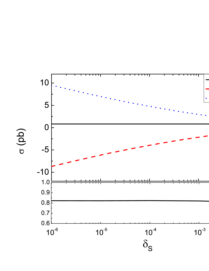
In Fig. 4, we show the dependence of the NLO cross sections on the cutoffs and . In fact, the soft-collinear and the hard-noncollinear parts individually strongly depend on the cutoffs. But the total cross section is independent on cutoffs after all pieces are added together. From Fig. 4, we can see that the change of is very slow for in the range from to , which indicates that it is reasonable to use the two cutoff phase space slicing method.
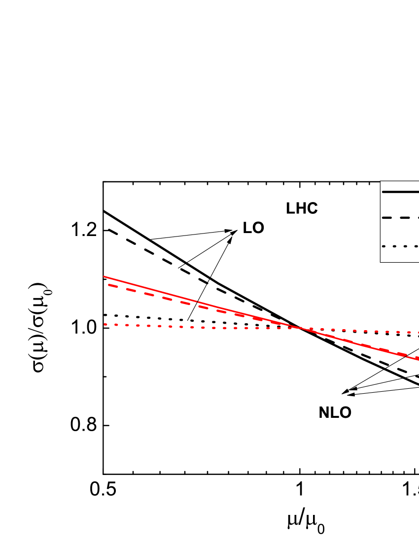
In Fig. 5, we give the scale dependences of the LO and NLO total cross sections. Explicitly, we consider three cases: factorization scale dependence ( and ); renormalization scale dependence ( and ); total scale dependences (). From Fig. 5, we find that the NLO corrections significantly reduce the scale dependences for all three cases, which makes the theoretical predictions more reliable.
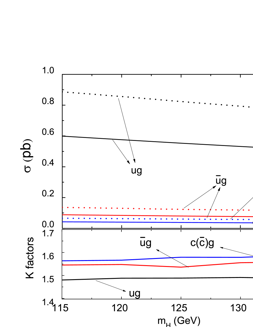
Figure 6 presents the dependence of the total cross sections on . It can be seen that the cross sections decrease by about as increases from GeV to GeV. In Fig. 6, the K factors, defined as , are also shown. We can see that the K factors for , and processes are , and , respectively, at the LHC for GeV, and they are not sensitive to the Higgs boson mass.
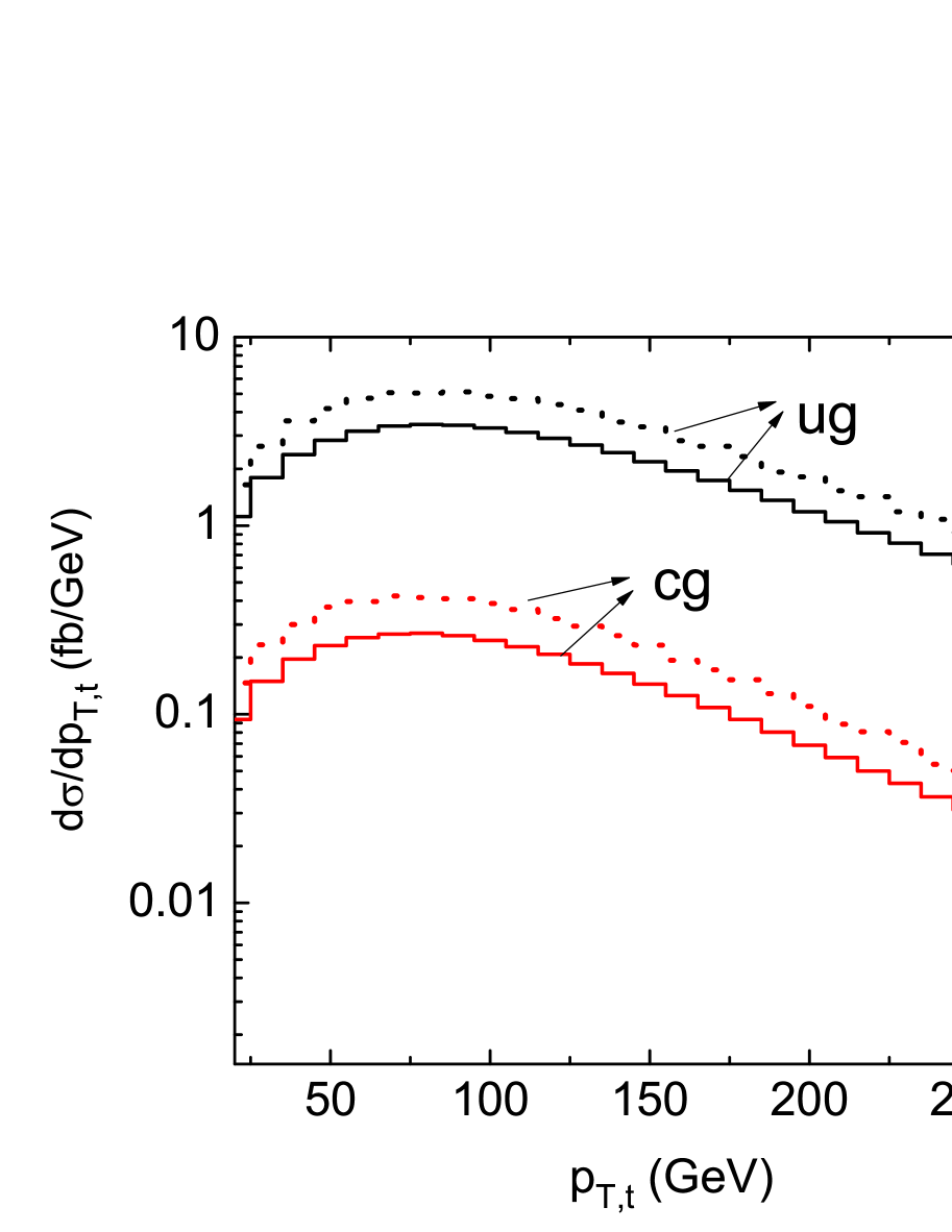
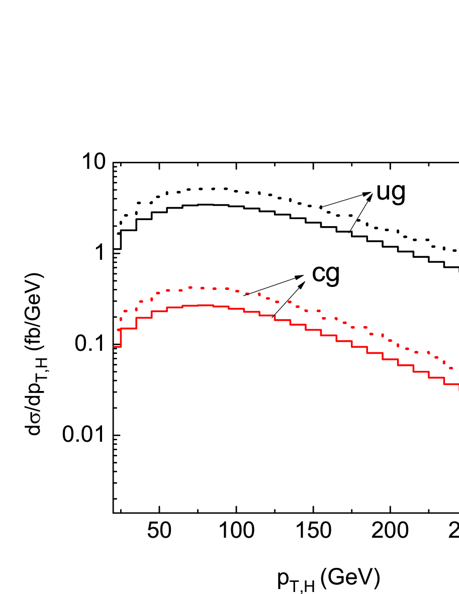
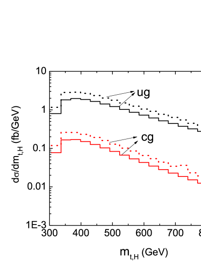
Figure 7 shows the differential cross sections as a function of the transverse momentum of the top quark and the Higgs boson. We find that they are very similar and the peak positions are around . In Fig. 8, we present the distributions of the invariant mass of the top quark and Higgs boson, and the peaks are around . From these figures, we can see that the NLO corrections significantly increase the LO results, but do not change the distribution shapes.
V Signal and discovery potentiality
In this section, we investigate the signal and corresponding backgrounds in detail and present the discovery potential of the signal of the associated production at the LHC.
V.1 NLO prediction on FCNC associated production and decay
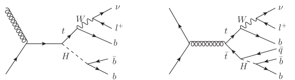
We have discussed the QCD NLO corrections to associated production in the last section. In order to provide a complete QCD NLO prediction on the signal, we need to include the QCD NLO corrections to the decay of the top quark and the Higgs boson. In this work, we concentrate on the top quark semileptonic decay and the Higgs boson decaying to , as shown in Fig. 9.
The complete NLO cross section for associated production and decay can be written as
| (45) |
where is the LO contribution to the associated production rate, are the LO total top quark and Higgs boson decay width, and are the decay width of the top quark decaying into and the Higgs boson decaying into . and , with , are the corresponding NLO corrections. We choose , . And we calculate width of the Higgs boson by Bridge at the LO Meade and Reece (2007), and adopt NLO results in Ref. Denner et al. (2011). Here we use the modified narrow width approximation (MNW) incorporating the finite width effects as the treatment in Refs. Cao et al. (2005b); Campbell et al. (2004).
We expand Eq. (45) to order ,
| (46) | |||||
Now we can separate QCD NLO corrections into three classes, i.e., the associated production at the NLO with subsequent decay at the LO, production at the LO with subsequent decay at the NLO, and production and decay at the LO but having NLO corrections from MNW. We note that QCD NLO corrections to the top quark decay part will contribute little since the branching ratio of the top quark decaying into boson is always Gao et al. (2011). As a consequence, the third term and the fourth term of Eq. (46) almost cancel each other. Since we only consider one decay mode of Higgs bosons, the sum of the fifth term and the sixth term will give a negative contribution.
There is another process, which is at the same order as the associated production at the NLO (Fig. 9 (Right)), i.e., production with the top quark semilepton decay and the antitop decaying into via FCNC vertex. It has the same signal if the light quark from the top quark is missed by the detector. This additional contribution is very significant for detecting the couplings, because the process is suppressed by quark PDF.
V.2 Collider simulation
To account for the resolution of the detectors, we apply energy and momentum smearing effects to the final states Aad et al. (2009):
| (47) |
where are the energy of the lepton, jet and the other jets, respectively.
We use the anti- jet algorithm Cacciari et al. (2008) with the jet radius and require the final-state particle to satisfy the following basic kinematic cuts
| (48) |
Here is the missing transverse energy. and are the transverse momentum and pseudorapidity of the jet, other quark jets and leptons, respectively. And stands for the angular distance. Moreover, we choose a -tagging efficiency of 0.6 for jets and mistagging rates of 1% for other quarks.
V.3 Events selection
The main background arises from the production with one top quark leptonic decay and the other top quark hadronic decay. Other backgrounds include , and production processes. These backgrounds are calculated at the LO by using the MADGRAPH4 Alwall et al. (2007) and ALPGEN Mangano et al. (2003) programme.
For the signal, we require three tagged jets , a lepton and the missing energy in the final states at both LO and NLO. When considering the number and kind of the final-state jets after jet clustering, there are several cases as follows:
(1) Fewer than three exclusive jets where two jets are combined together. We discard such events.
(2) Three exclusive jets. It can be from the LO and virtual corrections, which have three bottom quarks in the final states. The final states of real corrections can also give three jets if the additional emitted parton is combined into one of the jets. As a result, some combination procedure of jets may be different from the real partonic process. For example, the additional gluon comes from the initial states or the top quark decay, but it is combined into the jets arising from the Higgs boson, which will change the reconstructed particle mass spectrum.
(3) Four exclusive jets where the additional jet comes from a gluon or light quark. We only use the three tagged jets, neglecting the additional jet, in the final states to reconstruct the top quark and the Higgs boson. If the additional jet comes from the decay process, the reconstructed particle mass will be lower than the exact value due to lack of the momentum of the additional jet.
(4) Four exclusive jets where the additional jet comes from a quark. If all of these jets are tagged, we must distinguish which one is the additional jet. But the cross section for such process is strongly suppressed by the quark PDF, this contribution is neglectable.
The momentum of neutrino can be obtained by solving the on shell mass-energy equation of the boson
| (49) |
where is the momentum of the lepton, and is the reconstructed boson mass. We denote the longitudinal and transverse momentum of the neutrino as and , respectively. Since we generate intermediated particles with the MNW method, the masses of the intermediated particles change with Breit-Weinger distribution in a region of twenty times of their widthes around the central value set in Eq. (IV.2). At the same time, smearing effects on the final-state particles also affect the reconstructed mass. As a result, if we choose a low mass of boson, there may be no solution for in Eq. (49). So we must estimate a boson mass, which is large enough to provide the solution of mass-energy equation and small enough to reconstruct the proper top quark mass. Since there are three jets in the final states, it is necessary to determine the proper combination of the jets to reconstruct the top quark mass and the Higgs boson mass . In practice, we adopt the following steps:
(1) We choose randomly with Breit-Weinger distribution when solving Eq. (49) to get the neutrino longitudinal momentum. For such , it is required to provide real solutions of the equation. If not, discard this value of and redo this step until we obtain real solutions.
(2) In order to improve the boson reconstruction efficiency and save calculation time, we repeat step 1 for ten times and denote the solutions as , with . The superscript represents the number of the solutions in Eq. (49).
(3) Choose one momentum of the jets and one of to reconstruct the top quark mass .
(4) For all combinations of , we choose the best one to minimize .
(5) Use the remnant jets to reconstruct Higgs boson mass .
In order to choose appropriate kinematic cuts, we show some important kinematic distributions for the signal and the backgrounds.
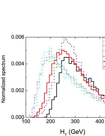
In Fig. 10, we present dependence of differential cross sections of the signal and backgrounds on , defined as the scalar sum of lepton and jet transverse momenta. From the figure, we can see that the distributions of , and backgrounds have peaks below GeV, while the peak positions of the signals are about GeV. Therefore we choose the cut
| (50) |
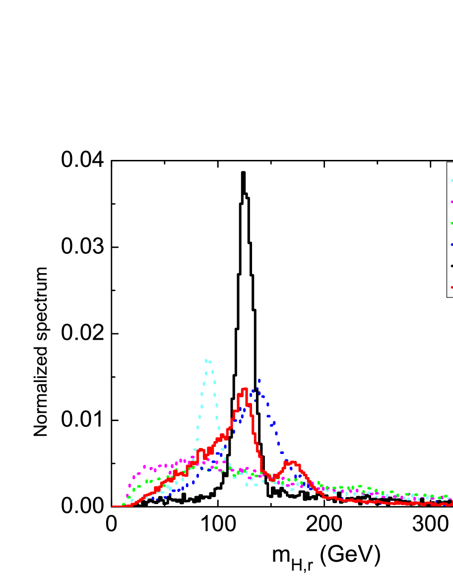
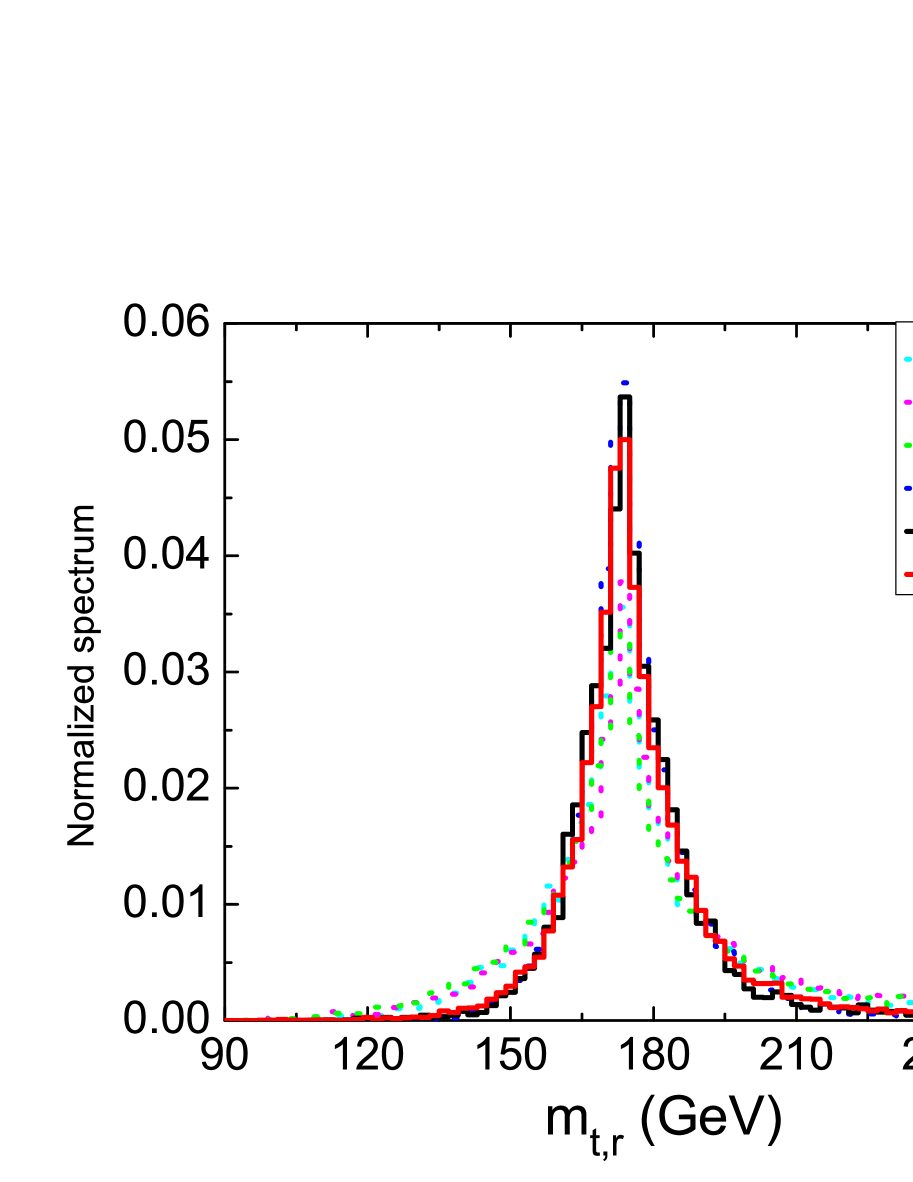
Figure 11 illustrates the distribution of the reconstructed Higgs boson mass of the signal and backgrounds. We can see that the signals have peaks around 125 GeV, while the distributions of backgrounds are continuous or have peaks at other places. In order to suppress , and backgrounds, we require the mass of the Higgs boson to satisfy
| (51) |
where is defined as . The reason will be explained in more detail in the Appendix. We also show the distribution of the reconstructed top quark mass in Fig. 11, where the signal and the backgrounds have similar distributions. As a result, we choose the cut
| (52) |
to keep more signal events, where is defined as .
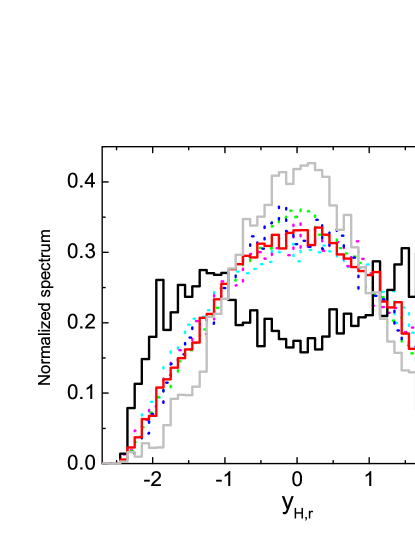
To determine the rapidity cut, we present the normalized spectrum of the rapidity of the reconstructed resonances for the signal and backgrounds in Fig. 12. It can be seen the Higgs boson from the associated production concentrates in the forwards and backwards regions. This is due to the fact that the momentum of initial quark is generally larger than that of gluon, so the partonic center-of-mass frame is highly boosted along the direction of the quark. On the contrary, the main contribution of top pair production comes from gluon initial-states, which are symmetric and have small boost effect. So we impose rapidity cut on reconstructed Higgs boson for the signal of process as
| (53) |
However, since quark is the sea quark, the momentum of initial quark is much smaller than that of the initial quark. As a result, the Higgs boson from initial states is not boosted as from initial states. In addition, the cross section of decay is comparable to that of process. Therefore when discussing the couplings, we do not apply the cut in Eq. (53).
The complete set of kinematical cuts is listed in Table 2.
| basic cut | GeV, GeV, GeV, | ||
| GeV | |||
| GeV | |||
| GeV | |||
V.4 Simulation results
In this subsection, we discuss the numerical results after imposing kinematic cuts. We need to include the QCD NLO corrections to the decay as well. As a result, we find that these corrections reduce the cross sections by about 50% for the coupling induced process and by about for the coupling induced process, respectively. The corresponding results are listed in Table 3. only includes the NLO corrections to the associated production, while also contains the NLO corrections to decay. The complete QCD NLO corrections are for and almost vanish for .
| [fb] | |||
|---|---|---|---|
| 6.64 | 1.22 | 1.11 | |
| 0.428 | 1.40 | 1.00 |
| basic cut | ||||||
|---|---|---|---|---|---|---|
| (NLO) | 3.54 | 3.26 | 2.86 | 2.22 | 1.59 | 44.9% |
| (NLO) | 0.40 | 0.354 | 0.322 | 0.240 | 0.09 | 22.5% |
| (LO) | 0.993 | 0.956 | 0.849 | 0.487 | 0.193 | 19.4% |
| 21.0 | 19.9 | 17.3 | 9.55 | 3.89 | 18.5% | |
| 3.30 | 2.32 | 1.38 | 0.336 | 0.146 | 4.4% | |
| 0.215 | 0.160 | 0.099 | 0.023 | 0.010 | 4.7% | |
| 0.085 | 0.064 | 0.038 | 0.009 | 0.004 | 4.7% |
We list the results after imposing various kinematic cuts in Table 4. For the process, the clear signal with the coupling can be observed at the C.L. when the integrated luminosity is at the LHC. Here we define the discovery significance as and exclusion limits as , where and are the expected events numbers of the signal and the backgrounds. However, for the process, the cross section of the process is about 2 times larger than that of the process after cuts. As stated before, we choose data from the fifth column of Table 4. As a result, the C.L. discovery sensitivity of is 0.294 when the integrated luminosity is and GeV.


We show the discovery sensitivities to FCNC couplings with several Higgs boson mass for different luminosities in Fig. 13. For a lighter Higgs boson, the cross sections become larger, but the branching ratio rates of get lower. When GeV and integrated luminosity is , the limit on the coupling is 15% smaller than that for GeV. In contrast, when the Higgs boson mass increases to GeV, the limit is increased by 12.3%. The coupling has the similar behavior.
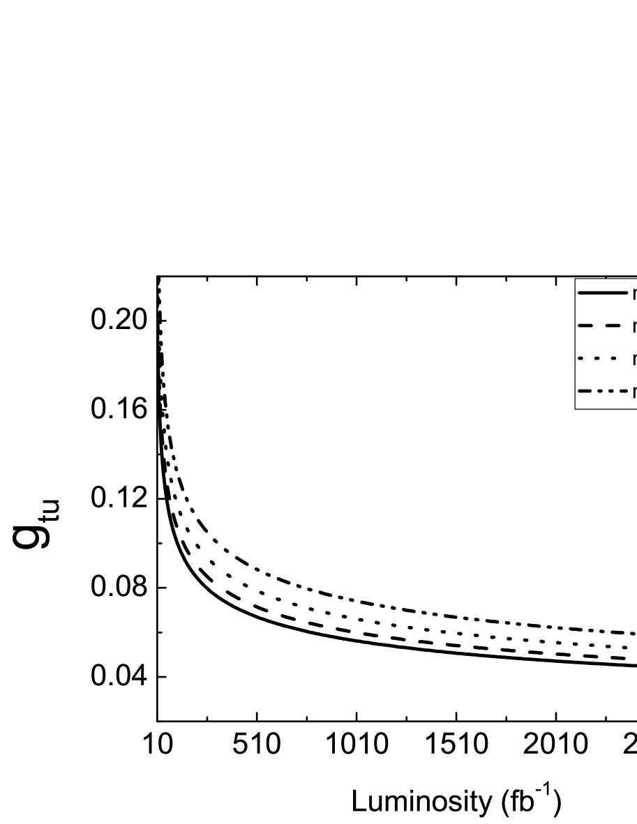
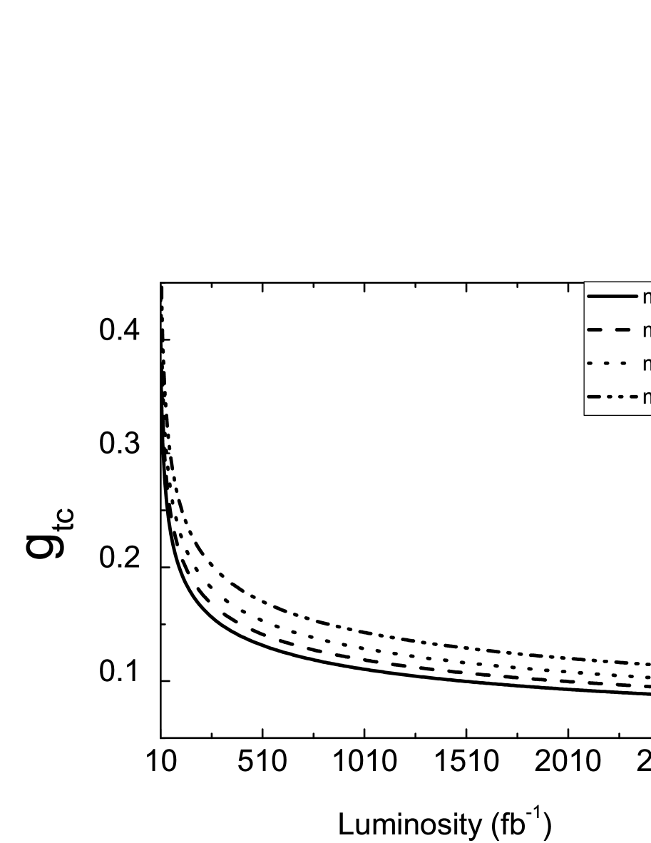
If no signal is observed, it means that the FCNC couplings can not be too large. In Fig. 14, we show the exclusion limits of couplings with several Higgs boson masses for different luminosities. The upper limits on the size of FCNC couplings are given as and with GeV. These limits can be converted to the C.L. upper limits on the branching ratios of top quark rare decays Li et al. (1991); Aguilar-Saavedra (2004) as follows:
| (54) |
VI CONCLUSION
In conclusion, we have investigated the signal of the associated production via the FCNC couplings at the LHC with TeV, including complete QCD NLO corrections to the production and decay of top quark and Higgs boson. Our results show that the NLO corrections reduce the scale dependences of the total cross sections, and increase the production cross sections by and for the and couplings induced processes, respectively. After kinematic cuts are imposed on the decay products of the top quark and the Higgs boson, the NLO corrections are reduced to for the coupling induced process and almost vanish for the coupling induced process. For the signal, we discuss the Monte Carlo simulation results for the signal and corresponding backgrounds, including the process of top quark pair production with one of the top quarks decaying to as well, and show that the NP signals may be observed at the level in some parameter regions. Otherwise, the upper limits on the FCNC couplings can be set, which can be converted to the constraints on the top quark rare decay branching ratios.
VII Acknowledgements
This work was supported by the National Natural Science Foundation of China, under Grants No. 11021092, No. 10975004 and No. 11135003.
APPENDIX
In this appendix, we numerically check the mass cut of the reconstructed particles. As stated before, the emission of an extra gluon broadens the mass distributions of reconstructed particles and makes -jet softer, which decreases the K factor of QCD NLO corrections when imposing reconstructing mass cuts or -jet cuts. The more strict mass cuts are imposed, the smaller cross sections we get. On the contrary, if the mass cuts are loose, though the cross sections are larger, more background events are also be considered, which may decrease the signal to background ratio. As a result, it is difficult to choose mass cuts on the reconstructed particles. We have checked that when we change from GeV to GeV, the sensitivity to the coupling at the level is the lowest when GeV, as shown in Table 5. It confirms our choice in Eq. (51).
| GeV | GeV | GeV | GeV | GeV | |
|---|---|---|---|---|---|
| sensitivity to | 0.180 | 0.159 | 0.157 | 0.150 | 0.335 |
References
- Chatrchyan et al. (2012) S. Chatrchyan et al. (CMS Collaboration), Phys.Lett.B (2012), eprint 1207.7235.
- Aad et al. (2012) G. Aad et al. (ATLAS Collaboration), Phys.Lett. B716, 1 (2012), eprint 1207.7214.
- Glashow et al. (1970) S. Glashow, J. Iliopoulos, and L. Maiani, Phys.Rev. D2, 1285 (1970).
- Blankenburg et al. (2012) G. Blankenburg, J. Ellis, and G. Isidori, Phys.Lett. B712, 386 (2012), eprint 1202.5704.
- Aguilar-Saavedra (2004) J. Aguilar-Saavedra, Acta Phys.Polon. B35, 2695 (2004), eprint hep-ph/0409342.
- del Aguila et al. (1999) F. del Aguila, J. Aguilar-Saavedra, and L. Ametller, Phys.Lett. B462, 310 (1999), eprint hep-ph/9906462.
- Aguilar-Saavedra (2001) J. Aguilar-Saavedra, Phys.Lett. B502, 115 (2001), eprint hep-ph/0012305.
- Aguilar-Saavedra and Branco (2000) J. Aguilar-Saavedra and G. Branco, Phys.Lett. B495, 347 (2000), eprint hep-ph/0004190.
- Liu et al. (2005) J. J. Liu, C. S. Li, L. L. Yang, and L. G. Jin, Phys.Rev. D72, 074018 (2005), eprint hep-ph/0508016.
- Zhang et al. (2009) J. J. Zhang, C. S. Li, J. Gao, H. Zhang, Z. Li, et al., Phys.Rev.Lett. 102, 072001 (2009), eprint 0810.3889.
- Gao et al. (2009) J. Gao, C. S. Li, J. J. Zhang, and H. X. Zhu, Phys.Rev. D80, 114017 (2009), eprint 0910.4349.
- Zhang et al. (2011) Y. Zhang, B. H. Li, C. S. Li, J. Gao, and H. X. Zhu, Phys.Rev. D83, 094003 (2011), eprint 1101.5346.
- Li et al. (2011) B. H. Li, Y. Zhang, C. S. Li, J. Gao, and H. X. Zhu, Phys.Rev. D83, 114049 (2011), eprint 1103.5122.
- Yang (2005) J. M. Yang, Annals Phys. 316, 529 (2005), eprint hep-ph/0409351.
- Bejar et al. (2003) S. Bejar, J. Guasch, and J. Sola, Nucl.Phys. B675, 270 (2003), eprint hep-ph/0307144.
- Cao et al. (2005a) J.-j. Cao, G.-l. Liu, and J. M. Yang, Eur.Phys.J. C41, 381 (2005a), eprint hep-ph/0311166.
- Guasch and Sola (1999) J. Guasch and J. Sola, Nucl.Phys. B562, 3 (1999), eprint hep-ph/9906268.
- Bejar et al. (2001) S. Bejar, J. Guasch, and J. Sola, Nucl.Phys. B600, 21 (2001), eprint hep-ph/0011091.
- Yang and Li (1994) J.-M. Yang and C.-S. Li, Phys.Rev. D49, 3412 (1994).
- de Divitiis et al. (1997) G. de Divitiis, R. Petronzio, and L. Silvestrini, Nucl.Phys. B504, 45 (1997), eprint hep-ph/9704244.
- Diaz-Cruz et al. (2002) J. Diaz-Cruz, H.-J. He, and C. Yuan, Phys.Lett. B530, 179 (2002), eprint hep-ph/0103178.
- Cao et al. (2006) J. Cao, G. Eilam, K.-i. Hikasa, and J. M. Yang, Phys.Rev. D74, 031701 (2006), eprint hep-ph/0604163.
- Gaitan et al. (2006) R. Gaitan, O. Miranda, and L. Cabral-Rosetti, AIP Conf.Proc. 857, 179 (2006), eprint hep-ph/0604170.
- Arhrib and Hou (2006) A. Arhrib and W.-S. Hou, JHEP 0607, 009 (2006), eprint hep-ph/0602035.
- Fernandez et al. (2010) A. Fernandez, C. Pagliarone, F. Ramirez-Zavaleta, and J. Toscano, J.Phys.G G37, 085007 (2010), eprint 0911.4995.
- Aranda et al. (2010) J. Aranda, A. Cordero-Cid, F. Ramirez-Zavaleta, J. Toscano, and E. Tututi, Phys.Rev. D81, 077701 (2010), eprint 0911.2304.
- Larios et al. (2005) F. Larios, R. Martinez, and M. Perez, Phys.Rev. D72, 057504 (2005), eprint hep-ph/0412222.
- Plehn (2003) T. Plehn, Phys.Rev. D67, 014018 (2003), eprint hep-ph/0206121.
- Weydert et al. (2010) C. Weydert, S. Frixione, M. Herquet, M. Klasen, E. Laenen, et al., Eur.Phys.J. C67, 617 (2010), eprint 0912.3430.
- Zhu (2003) S.-h. Zhu, Phys.Rev. D67, 075006 (2003), eprint hep-ph/0112109.
- Klasen et al. (2012) M. Klasen, K. Kovarik, P. Nason, and C. Weydert (2012), eprint 1203.1341.
- Harris and Owens (2002) B. Harris and J. Owens, Phys.Rev. D65, 094032 (2002), eprint hep-ph/0102128.
- Zhang et al. (2010) J. J. Zhang, C. S. Li, J. Gao, H. X. Zhu, C.-P. Yuan, et al., Phys.Rev. D82, 073005 (2010), eprint 1004.0898.
- Passarino and Veltman (1979) G. Passarino and M. Veltman, Nucl.Phys. B160, 151 (1979).
- Denner (1993) A. Denner, Fortsch.Phys. 41, 307 (1993), eprint 0709.1075.
- Ellis and Zanderighi (2008) R. K. Ellis and G. Zanderighi, JHEP 0802, 002 (2008), eprint 0712.1851.
- Collins et al. (1985) J. C. Collins, D. E. Soper, and G. F. Sterman, Nucl.Phys. B261, 104 (1985).
- Bodwin (1985) G. T. Bodwin, Phys.Rev. D31, 2616 (1985).
- Carena et al. (2000) M. S. Carena, D. Garcia, U. Nierste, and C. E. Wagner, Nucl.Phys. B577, 88 (2000), eprint hep-ph/9912516.
- Meade and Reece (2007) P. Meade and M. Reece (2007), eprint hep-ph/0703031.
- Denner et al. (2011) A. Denner, S. Heinemeyer, I. Puljak, D. Rebuzzi, and M. Spira, Eur.Phys.J. C71, 1753 (2011), eprint 1107.5909.
- Cao et al. (2005b) Q.-H. Cao, R. Schwienhorst, and C.-P. Yuan, Phys.Rev. D71, 054023 (2005b), eprint hep-ph/0409040.
- Campbell et al. (2004) J. M. Campbell, R. K. Ellis, and F. Tramontano, Phys.Rev. D70, 094012 (2004), eprint hep-ph/0408158.
- Gao et al. (2011) J. Gao, C. S. Li, L. L. Yang, and H. Zhang, Phys.Rev.Lett. 107, 092002 (2011), eprint 1104.4945.
- Aad et al. (2009) G. Aad et al. (ATLAS Collaboration) (2009), eprint 0901.0512.
- Cacciari et al. (2008) M. Cacciari, G. P. Salam, and G. Soyez, JHEP 0804, 063 (2008), eprint 0802.1189.
- Alwall et al. (2007) J. Alwall, P. Demin, S. de Visscher, R. Frederix, M. Herquet, et al., JHEP 0709, 028 (2007), eprint 0706.2334.
- Mangano et al. (2003) M. L. Mangano, M. Moretti, F. Piccinini, R. Pittau, and A. D. Polosa, JHEP 0307, 001 (2003), eprint hep-ph/0206293.
- Li et al. (1991) C. S. Li, R. J. Oakes, and T. C. Yuan, Phys.Rev. D43, 3759 (1991).