Parity anomaly and Landau-level lasing in strained photonic honeycomb lattices

Abstract

We describe the formation of highly degenerate, Landau-level-like amplified states in a strained photonic honeycomb lattice in which amplification breaks the sublattice symmetry. As a consequence of the parity anomaly, the zeroth Landau level is localized on a single sublattice and possesses an enhanced or reduced amplification rate. The spectral properties of the higher Landau levels are constrained by a generalized time-reversal symmetry. In the setting of two-dimensional photonic crystal lasers, the anomaly directly affects the mode selection and lasing threshold while in three-dimensional photonic lattices it can be probed via beam dynamics.

Nonuniform deformations of the honeycomb lattice of graphene result in a pseudomagnetic field which deflects particles in analogy to the Lorentz force, with small amounts of strain producing fields that are large enough to create well-defined Landau levels in the low-energy range of the spectrum, in absence of any physical magnetic field guinea ; vozmediano ; levy ; yan . Here we describe how the addition of gain in an analogous photonic setting results in the formation of highly degenerate amplifying Landau levels, which can provide the platform for a laser with macroscopic mode competition. The spectral properties of these levels become intriguing when the gain breaks the sublattice symmetry. Due to the parity anomaly jackiw ; semenoff ; haldane , the amplification of the zeroth Landau level is dictated by one of the two sublattices, which here is selected depending on the strain orientation. Moreover, a reflection symmetry enforces that the instances of this level in the two $\mathbf{k}$-space valleys behave identically. In contrast, the higher Landau levels are constrained by a generalized time-reversal symmetry. Their amplification rate equals the average rate on the two sublattices, up to a finite threshold of the imbalance at which two levels coalesce and their rates bifurcate.

These observations allow to detect the parity anomaly via the anomalous amplification or decay of the zeroth Landau level. When the system is operated as a two-dimensional photonic crystal laser, the lasing threshold is set either by the zeroth or by the first Landau level, with the selection dictated by the strain orientation and signature of the amplification imbalance. We also describe how the anomalous behavior of the zeroth Landau level can be probed via the beam dynamics in a three-dimensional photonic lattice.

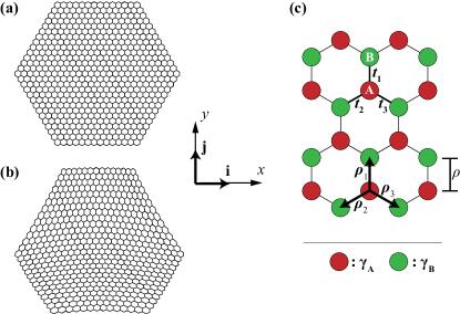
Figure 1: (Color online) (a) Segment of a honeycomb lattice, with vertices representing states in a two-dimensional photonic crystal or weakly coupled optical fibers in a three-dimensional setting. (b) Sketch of a deformed arrangement which results in a constant pseudomagnetic field. (c) We investigate the interplay of this field with amplification and absorption that breaks the sublattice symmetry. The two sublattices A and B have amplification rates $\gamma_{A}$ and $\gamma_{B}$, respectively (negative values correspond to absorption). The pseudomagnetic field resulting from the strain is modeled via smooth coupling functions $t_{l}$ whose definition (5) involves the bond vectors $\boldsymbol{\rho}_{l}$, $l=1,2,3$.

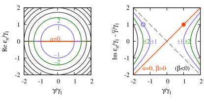
Figure 2: (Color online) Dependence of the Landau level spectrum (10), (13) on the amplification imbalance $\gamma=(\gamma_{A}-\gamma_{B})/2$, for strain leading to a pseudomagnetic field of strength $\beta$. (a) Real part, which vanishes for the zeroth Landau level, as well as for the other Landau levels beyond their bifurcation thresholds $\gamma_{n}$, Eq. (14). (b) Imaginary part, which becomes finite beyond the bifurcation. Because of the parity anomaly, the zeroth Landau level breaks the symmetry of the spectrum as it is located on the A sublattice for $\beta>0$ (thick solid line) while it is located on the B sublattice for $\beta<0$ (thin dashed line). The circles indicate the lasing threshold when $|\gamma|$ is increased at fixed average absorption $\bar{\gamma}=-\gamma_{1}$. For $\gamma>0$ this threshold is set by the zeroth Landau level, $\gamma_{L}=\gamma_{1}$ (solid circle), while for $\gamma<0$ it is set by the first Landau level, $\gamma_{L}=-\sqrt{2}\gamma_{1}$ (open circle).

Model of a strained active photonic honeycomb lattice.—We specifically consider the photonic system sketched in Fig. 1. Panel (a) shows a segment of a honeycomb lattice, with vertices representing weakly coupled optical fibers in a three-dimensional photonic lattice peleg or a set of basis states for a suitable spectral range in a two-dimensional photonic crystal pc ; raghu . The honeycomb lattice consists of two sublattices, A sites and B sites, which we equip with different amplification or absorption rates. This is motivated by recent works on optical realizations makris ; experiment1a ; experiment1b ; tachyons ; ramezani ; Regensburger of non-hermitian $\mathcal{PT}$-symmetric quantum mechanics bender . In the present setting, $\mathcal{P}$ stands for the inversion about the center of a hexagon, which maps A sites to B sites and thus inverts the amplification imbalance; $\mathcal{T}$ corresponds to complex conjugation and converts amplification into absorption, which also inverts the imbalance. Panel (b) sketches an inversion-symmetry-breaking deformed arrangement which results in a constant pseudomagnetic field whose interplay with the symmetry-breaking effects of amplification and absorption we are interested in. Panel (c) illustrates the microscopic modeling of these effects. The sublattices carry amplification rates $\gamma_{A}=\bar{\gamma}+\gamma$ and $\gamma_{B}=\bar{\gamma}-\gamma$, respectively, where $\bar{\gamma}$ is the average rate and $\gamma$ quantifies the imbalance. The rates $\gamma_{A}$ and $\gamma_{B}$ may be negative, in which case they signify absorption. Strain results in a spatial variation of the coupling terms $t_{ab}$ between neighboring A and B sites, which we parameterize as $t_{ab}=t_{l}(\mathbf{r}_{a})$, where $\mathbf{r}_{a}$ is the unstrained position of the A site and $l=1,2,3$ indicates the orientation along the unstrained bond vectors $\boldsymbol{\rho}_{l}$ ($|\boldsymbol{\rho}_{l}|=\rho$ is the unstrained nearest-neighbor distance). The typical magnitude of the coupling terms is denoted as $t_{0}$.

We focus on a spectral range where the unstrained passive lattice displays a conical band structure raghu . Based on the descriptions of strained graphene guinea ; vozmediano ; wallace ; Sasaki ; saito and photonic honeycomb lattices or crystals peleg ; pc ; raghu ; makris ; experiment1a ; experiment1b ; tachyons ; ramezani , the resulting Lorentz force and the effects of amplification and absorption are then captured by a Dirac equation with Hamiltonian supmat

$$\mathcal{H}=\left(\begin{array}[]{cc}i\gamma_{A}&v(\sigma P_{x}-iP_{y})\\ v(\sigma P_{x}+iP_{y})&i\gamma_{B}\end{array}\right),$$ (1)

$v=3t_{0}\rho/2$, $P_{x}=-i\partial_{x}-A_{x}$, $P_{y}=-i\partial_{y}-A_{y}$, where

$$\mathbf{A}=\sigma\frac{1}{3\rho t_{0}}(2t_{1}-t_{2}-t_{3})\mathbf{i}+\sigma\frac{1}{\sqrt{3}\rho t_{0}}(t_{2}-t_{3})\mathbf{j}$$ (2)

is the pseudomagnetic vector potential. This Hamiltonian applies to a continuous spinor wave function $(\varphi_{A}(\mathbf{r}),\varphi_{B}(\mathbf{r}))^{T}$ which is obtained by separating out rapid fluctuations with wave vector $\mathbf{K}_{\sigma}=\sigma(4\pi/3\sqrt{3}\rho)\mathbf{i}$, $\sigma=\pm 1$, where $\sigma$ distinguishes two independent valleys; these valleys are related by the $\mathcal{P}$ and $\mathcal{T}$ symmetries of the unstrained passive system raghu . The eigenvalues $\varepsilon$ of ${\cal H}$ determine the frequencies $\omega$ of quasibound states in the two-dimensional setting pc ; raghu or the propagation constant $ck_{z}$ along the third direction in the three-dimensional setting peleg ; makris . Eigenvalues with a positive imaginary part correspond to amplified states (in time or along the propagation direction), while those with a negative imaginary part correspond to decaying states.

Before we turn to the effects of the pseudomagnetic field let us inspect some limits. For vanishing $\gamma_{A}=\gamma_{B}=0$ and constant $t_{ab}=t_{0}$, the system is periodic and the band structure displays the familiar Dirac cones $\varepsilon=\pm v|\mathbf{q}|$ near each corner of the Brillouin zone (the K and K^′ points situated at $\mathbf{K}_{+}$ and $\mathbf{K}_{-}$, respectively), where $\mathbf{q}=\mathbf{k}-\mathbf{K}_{\sigma}$ is the wave vector relative to the corner point wallace . Weak uniform strain, with $t_{ab}=t_{1,2,3}$ only depending on the bond orientation, displaces the cones from the corners by an amount ${\bf A}$ Sasaki ; saito . In the presence of amplification and absorption with $\gamma_{A}=-\gamma_{B}=\gamma$, the full band structure of the uniformly strained system can still be real since in this case the non-hermitian Hamiltonian (1) displays the $\mathcal{PT}$ symmetry

$$\mathcal{H}(x,y)=\sigma_{x}\mathcal{H}^{*}(-x,-y)\sigma_{x}\equiv\mathcal{PT}H(x,y)\mathcal{PT},$$ (3)

where $\sigma_{x}$ is the Pauli matrix. However, when $\gamma$ exceeds a threshold eigenstates cease to be joint eigenstates of $\mathcal{PT}$, which leads to complex branches of the band structure ramezani ; tachyons . If amplification and absorption are imbalanced, all eigenvalues are shifted by $i\bar{\gamma}$. This includes the case of ‘passive’ $\mathcal{PT}$ symmetry, where $\bar{\gamma}=-|\gamma|$ such that one sublattice is absorbing and the other sublattice is neutral experiment1a . In these more general cases, a relaxed $\mathcal{PT}$ symmetry can be stated as

$$\mathcal{H}=\mathcal{PT}\mathcal{H}\mathcal{PT}+2i\bar{\gamma}.$$ (4)

The spectrum of such a system is constrained to eigenvalues which either fulfill ${\rm Im}\,\varepsilon_{n}=\bar{\gamma}$, or are paired with another eigenvalue $\varepsilon_{\bar{n}}=\varepsilon_{n}-2i{\rm Im}\,\varepsilon_{n}+2i\bar{\gamma}$. However, strain explicitly breaks the $\mathcal{PT}$ symmetry, as we explore in the following.

Landau levels.— We consider a strain configuration which results in a constant pseudomagnetic field of strength $\beta$. This follows from a smoothly varying three-fold symmetric configuration with guinea

$$t_{l}=t_{0}[1-(\beta/2)\boldsymbol{\rho}_{l}\cdot\mathbf{r}],\quad l=1,2,3,$$ (5)

which gives rise to a vector potential $\mathbf{A}=(\sigma\beta/2)(-y\mathbf{i}+x\mathbf{j})$. Microscopically $\beta$ depends on the sensitivity of the coupling terms on the nearest-neighbor spacing, as well as on the strain orientation; here we assume that this parameter is given. Assuming unless otherwise stated that $\beta>0$ we write the Hamiltonian as

$$\mathcal{H} =\left(\begin{array}[]{cc}i\gamma_{A}&v\sqrt{2\beta}\Pi^{\dagger}\\ v\sqrt{2\beta}\Pi&i\gamma_{B}\end{array}\right),$$ (8)

$$\Pi =\frac{1}{\sqrt{2\beta}}(-i\sigma\beta x/2-i\sigma\partial_{x}+\beta y/2+\partial_{y}),$$ (9)

where $[\Pi,\Pi^{\dagger}]=1$ coincides with the algebra of harmonic oscillator annihilation and creation operators. This delivers a spectrum of Landau levels, with the zeroth level given by

$$\phi_{0}=\left(\begin{array}[]{c}\chi_{0}\\ 0\end{array}\right),\quad\varepsilon_{0}=i\gamma_{A}=i\bar{\gamma}+i\gamma,$$ (10)

where $\chi_{0}=(\beta/2\pi)^{1/2}\exp[-\beta(x^{2}+y^{2})/4+\lambda(\sigma x+iy)-\lambda^{2}/\beta]$ represents the infinitely degenerate set of Landau states fulfilling $\Pi\chi_{0}=0$. With $\chi_{m}=(m!)^{-1/2}(\Pi^{\dagger})^{m}\chi_{0}$, $m=1,2,3,\ldots$, the other Landau levels are given by

$$\phi_{n} =\left(\begin{array}[]{c}\chi_{|n|}\\ \alpha_{n}\chi_{|n|-1}\end{array}\right),\,\,\varepsilon_{n}=i\bar{\gamma}+\mathop{\rm sgn}(n)\sqrt{\gamma_{n}^{2}-\gamma^{2}},$$ (13)

$$\alpha_{n} =\mathop{\rm sgn}(n)\sqrt{1-\frac{\gamma^{2}}{\gamma_{n}^{2}}}-i\frac{\gamma}{\gamma_{n}},\quad\gamma_{n}=\sqrt{2v^{2}\beta|n|},$$ (14)

for $n=\pm 1,\pm 2,\pm 3,\ldots$. This spectrum is shown in Fig. 2.

At vanishing $\gamma_{A,B}$ (thus $\bar{\gamma}=\gamma=0$), these solutions reduce to the strain-induced Landau levels studied in the graphene literature guinea ; vozmediano ; levy ; yan . For uniform amplification or absorption ($\gamma=0$), the levels are shifted by $i\bar{\gamma}$. For a finite amplification imbalance ($\gamma\neq 0$), the levels with index $n$ and $\bar{n}=-n$ (with $n\neq 0$) coalesce at a threshold value $|\gamma|=\gamma_{n}$ and then bifurcate into a pair of levels which fulfill the spectral constraints stipulated below Eq. (4); in particular, the average imaginary part of these eigenvalues is given by $i\bar{\gamma}$. The zeroth Landau level, however, has an imaginary part which differs from $\bar{\gamma}$, and is not accompanied by a partner state (not even in the other valley). This feature rules out the existence of any $\mathcal{PT}$-like antiunitary operator which would commute with the Hamiltonian.

The special nature of the zeroth Landau level can be seen as a direct consequence of the parity anomaly jackiw ; semenoff ; haldane , which in the present context is most conveniently identified by considering the supersymmetric interpretation of Hamiltonians of the form (8) jackiw . Depending on whether one eliminates the B site or A site wave function, the corresponding eigenvalue equation can be written as

$$(\varepsilon-i\gamma_{A})\varphi_{A} =(\varepsilon-i\gamma_{B})^{-1}2\beta v^{2}\Pi^{\dagger}\Pi\varphi_{A},$$ (15a)

$$(\varepsilon-i\gamma_{B})\varphi_{B} =(\varepsilon-i\gamma_{A})^{-1}2\beta v^{2}\Pi\,\Pi^{\dagger}\varphi_{B},$$ (15b)

which provides a simple example of supersymmetric partner potentials. Both equations deliver the same spectrum, except for the zeroth Landau level, which only occurs in the spectrum of Eq. (15a). This state thus breaks the sublattice symmetry—its wavefunction is localized on the A sublattice, and for $\gamma_{A}\neq\gamma_{B}$ this asymmetry is reflected by a departure from the overall symmetry of the spectrum about $i\bar{\gamma}$. This holds for $\beta>0$, as we have assumed so far. For $\beta<0$, one needs to modify the definitions of $\Pi$ and $\Pi^{\dagger}$ such that in the Hamiltonian (8) they are effectively interchanged, and the zeroth Landau level is localized on the B sublattice, with $\varepsilon_{0}=i\gamma_{B}$.

Focussing on a single valley (say around the K point, $\sigma=1$), this anomaly is fully analogous to the parity anomaly in the problem of massive Dirac electrons in a magnetic field, which possess an extra state located at energy $E=mc^{2}$ or $E=-mc^{2}$ (depending on the sign of the field) that breaks the symmetry of the spectrum about $E=0$ haldane . For electrons on an ordinary honeycomb lattice this anomaly is canceled in the K^′ point semenoff ; haldane , which can be related to the K point by either using the $\mathcal{P}$ symmetry (which interchanges the two sublattices) or the $\mathcal{T}$ symmetry (which inverts the magnetic field). In the present photonic setting the $\mathcal{T}$ operation relating the two valleys in $\mathbf{k}$-space inverts the sign of the amplification imbalance $\gamma$; furthermore, the $\mathcal{P}$ operation not only inverts $\gamma$ but also the direction of the vector potential (2)—thus, both symmetries are indeed broken. Instead, the Hamiltonian (8) can be mapped from one valley to the other by the reflection symmetry $x\to-x$, $\sigma\to-\sigma$. Therefore, the parity anomaly for the zeroth Landau level is replicated identically in both valleys.

We now turn to the other Landau levels. These are constrained by the chiral symmetry ${\cal H}(x,-y)^{*}=-{\cal H}(x,y)$, which results in the pairing $\varepsilon_{-n}=-\varepsilon_{n}^{*}$ of eigenvalues before the bifurcation threshold, $|\gamma|<\gamma_{n}$. The question now arises: Why do these levels also obey the spectral constraints that are usually associated with $\mathcal{PT}$-symmetric systems? In particular, before the bifurcation ${\rm Im}\,\varepsilon_{n}={\rm Im}\,\varepsilon_{-n}=\bar{\gamma}$ and the associated wave function (13) has equal weight on the A and B sublattices, $|\alpha_{n}|=|\alpha_{-n}|=1$. After the bifurcation, $|\alpha_{n}|=1/|\alpha_{-n}|\neq 1$, and the level with the larger imaginary part has a larger weight on the more amplifying sublattice, while the other state is predominantly localized on the opposite sublattice. These properties are all compatible with a existence of a generalized time-reversal symmetry $\widetilde{\mathcal{PT}}$ applying to these states.

To identify this symmetry we introduce the basis

$${|}m,A\rangle\equiv\left(\begin{array}[]{c}\chi_{m}\\ 0\end{array}\right),\quad{|}m,B\rangle\equiv\left(\begin{array}[]{c}0\\ \chi_{m}\end{array}\right),\quad m=0,1,2,\ldots$$

of ordinary Landau states localized on the A or B sublattice (we suppress the degeneracy of these levels). In this basis, the Hamiltonian (8) takes the form $\mathcal{H}=i\gamma_{A}{|}0,A\rangle\langle 0,A{|}+\widetilde{\mathcal{H}}$, where

$$\widetilde{\mathcal{H}}=\sum_{m=0}^{\infty}\Big{(}i\gamma_{A}{|}m+1,A\rangle\langle m+1,A{|}+i\gamma_{B}{|}m,B\rangle\langle m,B{|}$$

$$+v\sqrt{2\beta(m+1)}({|}m+1,A\rangle\langle m,B{|}+{|}m,B\rangle\langle m+1,A{|})\Big{)}$$

is the Hamiltonian in the subspace excluding the zeroth Landau level ${|}0,A\rangle$. Inspecting the properties of

$$\widetilde{\mathcal{P}} =\sum_{m=0}^{\infty}({|}m+1,A\rangle\langle m,B{|}+{|}m,B\rangle\langle m+1,A{|})$$ (16)

$$\widetilde{\mathcal{T}} :\Gamma|m,L\rangle\to\Gamma^{*}|m,L\rangle,\quad L=A,B,$$ (17)

in the original Hilbert space, we find $\widetilde{\mathcal{T}}^{2}=1$, $\widetilde{\mathcal{P}}^{\dagger}=\widetilde{\mathcal{P}}$, $\widetilde{\mathcal{P}}^{2}=1-{|}0,A\rangle\langle 0,A{|}$. Thus $\widetilde{\mathcal{PT}}\equiv\widetilde{\mathcal{P}}\widetilde{\mathcal{T}}|_{n\neq 0}$ is an antiunitary operator in the space of higher Landau levels. Furthermore, an explicit calculation now delivers the desired relation $\widetilde{\mathcal{H}}=\widetilde{\mathcal{PT}}\widetilde{\mathcal{H}}\widetilde{\mathcal{PT}}+2i\bar{\gamma}$ in the space of these levels, which entails the spectral constraints. This symmetry is of dynamical origin as its construction makes explicit reference to the eigenstates of the system. The symmetry does not extend to the zeroth Landau level since $\widetilde{\mathcal{P}}$ is not unitary if this state is included. While $\widetilde{\mathcal{P}}\widetilde{\mathcal{T}}\mathcal{H}=\mathcal{H}\widetilde{\mathcal{P}}\widetilde{\mathcal{T}}-2i\bar{\gamma}\widetilde{\mathcal{P}}\widetilde{\mathcal{T}}$, the relation $\widetilde{\mathcal{P}}\widetilde{\mathcal{T}}\mathcal{H}\widetilde{\mathcal{P}}\widetilde{\mathcal{T}}=\mathcal{H}-2i\bar{\gamma}-2i\gamma{|}0,A\rangle\langle 0,A{|}$ again reveals the special spectral status of this level.

Applications.— Our results for the complex spectrum of Landau levels find their natural applications in the lasing in a two-dimensional photonic crystal laserref1 ; laserref2 ; laserref3 ; laserref4 , and in the beam propagation in a photonic lattice peleg ; makris ; supmat .

We first consider the onset of lasing, which occurs when the system is realized in a two-dimensional photonic crystal, with negligible leakage into the perpendicular direction. The system becomes unstable towards lasing when the complex frequency of one of the Landau levels acquires a positive imaginary part. For fixed $\bar{\gamma}<0$, the system is passive at $\gamma=0$ (uniform absorption), but as $|\gamma|$ increases the zeroth Landau level changes its imaginary part, and so do the other Landau levels beyond their bifurcation thresholds $\gamma_{n}$. The lasing threshold $\gamma_{L}$ now depends on the sign of $\gamma$. If $\gamma>0$, the lasing threshold is given by $\gamma_{L}=|\bar{\gamma}|$ since the zeroth Landau level is then located on the amplifying sublattice. For $\gamma<0$, the first level to meet the real axis is associated with the pair $n=\pm 1$ involving the first Landau level, with lasing threshold $\gamma_{L}=\sqrt{2v^{2}\beta+\bar{\gamma}^{2}}$ [see Eq. (13)]. In the case $\bar{\gamma}=0$, the lasing threshold either vanishes (for $\gamma>0$) or is finite (for $\gamma<0$), depending on whether it is set by the zeroth or first Landau level. These considerations apply to the principal strain orientation studied here ($\beta>0$). If $\beta$ takes a negative value, the role of the two sublattices is interchanged and the zeroth Landau level becomes lasing for $\gamma<0$. Similar asymmetric threshold scenarios arise when one approaches lasing by changing $\bar{\gamma}$ at fixed $\gamma$, or when one changes the amplification rate on one sublattice only. In the lasing regime a macroscopic number of modes in the zeroth or first Landau level will participate in the mode competition. In a finite system, the exact degeneracy will be lifted by the boundary conditions, but this lifting will be small in the bulk, while edge states can also appear; disorder in the couplings and amplification rates will also broaden the levels.

When the system is realized in an array of single-mode waveguides the propagation along these waveguides is free, and the eigenvalues represent complex propagation constants, where the imaginary part describes the spatial decay or increase of the eigenmodes peleg ; makris ; supmat . An attractive feature of such settings is the possibility to probe the parity anomaly in a system without any active (amplifying) components. For this we set, e.g., $\gamma_{A}<0$ and $\gamma_{B}=0$, such that one sublattice is lossy while the other sublattice is passive. The parity anomaly can then be probed via a beam fed into one end of the waveguide array. The output beam will show the component of the zeroth Landau level either unaffected, or suppressed according to a decay constant $|\gamma_{A}|$. Assuming that $|\gamma_{A}|/2<\gamma_{1}$, all other components are suppressed uniformly according to a common decay constant $|\gamma_{A}|/2$. The initial population of the modes can be controlled via the input beam. This approach mirrors passive implementations of $\mathcal{PT}$-symmetric optics and avoids complications from the intrinsic dispersion in the active parts experiment1a ; experiment1b .

Conclusions.—In summary, we described the formation of Landau levels in a strained photonic system and identified means to probe the associated parity anomaly via amplification that breaks the sublattice symmetry. We focussed the attention on the honeycomb lattice as it naturally provides a conical dispersion, a pseudomagnetic field under strain, and two sublattices which can be equipped with gain and loss. It should be pointed out that conical dispersions are a generic feature of triangular lattices with inversion and time-reversal symmetry raghu , while the correspondence between strain and a pseudomagnetic field generalizes to other lattices iordanskii . Guided by coupled-mode theory peleg ; makris ; supmat one can identify a number of lattices with Dirac-like dispersions. Particularly promising variants include the Lieb lattice (a tripartite lattice which in addition exhibits a flat band) lieb and the one-dimensional Su-Schrieffer-Heeger chain ssh ; hs , a bipartite system which provides the platform for the recently reported $\mathcal{PT}$-symmetric Talbot effect talbot .

Note added.—We end by pointing the reader to recent experimental work on a passive photonic honeycomb lattice Rechtsman , which has shown that the three-fold symmetric strain pattern is indeed feasible and results in the formation of the Landau-levels described here.

Supplemental material: Parity anomaly and Landau-level lasing
in strained photonic honeycomb lattices

The argumentation in the main text is based on a Dirac-like wave equation (1) which incorporates gain, loss and nonuniform strain. Here we describe how this equation emerges from a microscopic model of a photonic honeycomb structure. We first focus on the technical details, which amount to a synthesis of works on graphene wallace ; Sasaki ; saito ; guinea ; vozmediano and $\mathcal{PT}$-symmetric lattices peleg ; makris ; experiment1a ; experiment1b ; tachyons ; ramezani ; Regensburger ; talbot ; Rechtsman , and then discuss the interpretation of the result.

As in these previous investigations we base the microscopic considerations on coupled-mode theory. In this theory, a tight-binding model is formulated on a lattice, where each vertex is associated with a localized mode while the bonds represent the coupling between the modes. This is illustrated in Fig. S3, which replicates Fig. 1 in the main text. Panel (a) shows a segment of a honeycomb lattice, consisting of two sublattices A and B. We denote the associated modes by $|a\rangle$, and $|b\rangle$, where the indices $a$ run over the A sublattice and the indices $b$ run over the B sublattice. Panel (b) sketches the deformed arrangement which results in a constant pseudomagnetic field. Panel (c) explains the microscopic modeling of these effects, which we elaborate in these supplemental notes. The modes on each sublattice are equipped with amplification or absorption rates $\gamma_{A}=\bar{\gamma}+\gamma$ and $\gamma_{B}=\bar{\gamma}-\gamma$. Here $\bar{\gamma}$ is the average rate and $\gamma$ quantifies the imbalance. We only consider nearest-neighbor couplings and denote the coupling rates as $t_{ab}$. In the unstrained case, $t_{ab}=t_{0}$ is constant. Strain results in a spatial variation of the coupling terms, which we parameterize as $t_{ab}=t_{l}(\mathbf{r}_{a})$, where $\mathbf{r}_{a}$ is the unstrained position of the A site and $l=1,2,3$ indicates the orientation along the unstrained bond vectors $\boldsymbol{\rho}_{l}$ (with $|\boldsymbol{\rho}_{l}|=\rho$ the unstrained nearest-neighbor distance). We orientate the lattice such that the orthogonal cartesian unit vectors $\mathbf{i}=(\boldsymbol{\rho}_{3}-\boldsymbol{\rho}_{2})/\sqrt{3}\rho$ and $\mathbf{j}=\boldsymbol{\rho}_{1}/\rho$.

Figure S3: Replication of Fig. 1 in the main text. (a) Segment of a honeycomb lattice, with vertices representing states in a two-dimensional photonic crystal or weakly coupled optical fibers in a three-dimensional setting. (b) Sketch of a deformed arrangement which results in a constant pseudomagnetic field. (c) The two sublattices A and B have amplification rates $\gamma_{A}$ and $\gamma_{B}$, respectively (negative values correspond to absorption). The pseudomagnetic field resulting from the strain is modeled via smooth coupling functions $t_{l}$ for bonds aligned along the vectors $\boldsymbol{\rho}_{l}$, $l=1,2,3$.

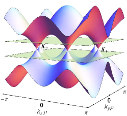
Figure S4: Dispersion of the unstrained passive honeycomb lattice in coupled-mode theory. The planes focus onto the central region, formed by cones with apex at the corners of the Brillouin zone (represented by the $\mathbf{K}_{+}$ and $\mathbf{K}_{-}$ points).

Based on the quantities introduced above, coupled-mode theory determines the eigenmodes $|\psi\rangle=\sum_{a}\psi_{a}|a\rangle+\sum_{b}\psi_{b}|b\rangle$ of the system as the eigenstates of an effective Hamiltonian

$$H=i\gamma_{A}\sum_{a}{|}a\rangle\langle a{|}+i\gamma_{B}\sum_{b}{|}b\rangle\langle b{|}-\sum_{{<}ab{>}}\!\!t_{ab}({|}a\rangle\langle b{|}+{|}b\rangle\langle a{|})$$ (S18)

(where the negative sign in front of the coupling terms follows convention). The eigenvalue equation is $\varepsilon|\psi\rangle=H|\psi\rangle$; the interpretation of the eigenvalues $\varepsilon$ depends on the context and is discussed towards the end of these notes.

We are interested in the modes of a system with smoothly varying coupling constants, in a spectral range close to the center of the dispersion of the unstrained passive system. The Dirac equation used in the text then arises in a gradient expansion in the lattice indices. To obtain the reference point for the expansion we set $t_{ab}=t_{0}$ and $\gamma_{A}=\gamma_{B}=0$. The eigenmodes are then of Bloch form

$$|\psi\rangle = \sum_{a}\phi^{(A)}\exp[i{\bf k}\cdot({\bf r}_{a}+\boldsymbol{\rho}_{1}/2)]|a\rangle$$ (S19)

$$+\sum_{b}\phi^{(B)}\exp[i{\bf k}\cdot({\bf r}_{b}-\boldsymbol{\rho}_{1}/2)]|b\rangle,$$

where we follow the convention to reference the lattice points to a suitably chosen center of a unit cell encompassing an A and a B site at the ends of a vertical bond. Inserting this ansatz into the eigenvalue equation one arrives at the Bloch Hamiltonian

$$\mathcal{H}=\left(\begin{array}[]{cc}0&-f\\ -f^{*}&0\\ \end{array}\right),$$ (S20)

where

$$f=t_{0}[1+e^{i\mathbf{k}\cdot(\boldsymbol{\rho}_{2}-\boldsymbol{\rho}_{1})}+e^{i\mathbf{k}\cdot(\boldsymbol{\rho}_{3}-\boldsymbol{\rho}_{1})}].$$ (S21)

The associated dispersion relation $\varepsilon=\pm|f({\bf k})|$, plotted in Fig. SS4, is conical in the center of the band, with the apex of each cone situated at a corner of the hexagonal Brillouin zone wallace . Only two of these $K$ points are independent, while the others are related by reciprocal lattice vectors. We set $\mathbf{K}_{\sigma}=\sigma(4\pi/3\sqrt{3}\rho)\mathbf{i}$ and distinguish the two independent choices by the valley index $\sigma=\pm 1$. Expanding the wave vector around these points, ${\bf k}={\bf K}_{\sigma}+{\bf q}$ with ${\bf q}=q_{x}{\bf i}+q_{y}{\bf j}$, one obtains

$$f \approx -\sigma vq_{x}+ivq_{y}$$ (S22)

where $v=\frac{3t_{0}\rho}{2}$. This delivers the conical dispersion $\varepsilon=v|{\bf q}|$ about the K points.

We now incorporate gain, loss and non-uniform but smooth strain within a gradient expansion, which captures these effects via a smooth envelope function that modulates the Bloch wave function. The full spatial dependence of the wave function is of the form

$$|\psi\rangle = \sum_{a}\phi^{(A)}({\bf r}_{a})\exp[i{\bf K}_{\sigma}\cdot({\bf r}_{a}+\boldsymbol{\rho}_{1}/2)]|a\rangle$$ (S23)

$$+\sum_{b}\phi^{(B)}({\bf r}_{b})\exp[i{\bf K}_{\sigma}\cdot({\bf r}_{b}-\boldsymbol{\rho}_{1}/2)]|b\rangle$$

where we separated the rapid oscillations with wave number ${\bf K}_{\sigma}$ from the slowly varying envelope functions $\phi^{(A)}({\bf r})$ and $\phi^{(B)}({\bf r})$. For the unstrained passive system, comparison with the expressions above delivers

$$\phi^{(A)}({\bf r}_{a}) =\phi^{(A)}\exp[i{\bf q}\cdot({\bf r}_{a}+\boldsymbol{\rho}_{1}/2)],$$

$$\phi^{(B)}({\bf r}_{b}) =\phi^{(B)}\exp[i{\bf q}\cdot({\bf r}_{b}-\boldsymbol{\rho}_{1}/2)],$$ (S24)

where $(\phi^{(A)},\phi^{(A)})^{T}$ is an eigenvector of the Bloch Hamiltonian (S20). The gradient expansion adapts these functions to the case of couplings $t_{ab}=t_{l}(\mathbf{r}_{a})$ with functions $t_{l}$, $l=1,2,3$, that vary smoothly across the lattice ($|\nabla t_{l}|\rho\ll t_{0}$). If these functions were constant we would arrive at the Bloch Hamiltonian (S20) with

$$f = t_{1}+t_{2}e^{i\mathbf{k}\cdot(\boldsymbol{\rho}_{2}-\boldsymbol{\rho}_{1})}+t_{3}e^{i\mathbf{k}\cdot(\boldsymbol{\rho}_{3}-\boldsymbol{\rho}_{1})}$$ (S25)

$$\approx -\sigma v(q_{x}-A_{x})+iv(q_{y}-A_{y}),$$

where we again expanded about a K point and abbreviated

$$A_{x}=\sigma\frac{1}{3t_{0}\rho}(2t_{1}-t_{2}-t_{3}),\quad A_{y}=\sigma\frac{1}{\sqrt{3}t_{0}\rho}(t_{2}-t_{3}).$$ (S26)

To capture the variations we insert Eq. (S23) into the eigenvalue equation of the microscopic coupled-mode Hamiltonian (S18) and determine the amplitudes of the neighboring unit cells via the Taylor expansion $\phi^{(A,B)}({\bf r}+\Delta{\bf r})\approx[1+\Delta{\bf r}\cdot\nabla]\phi^{(A,B)}({\bf r})$, where $\Delta\mathbf{r}$ is the lattice vector connecting the centers of the unit cells in question. Locally, the Hamiltonian is then still of the form (S20) with $f$ given as in (S25), but with $q_{x}\to p_{x}\equiv-i\partial_{x}$ and $q_{y}\to p_{y}\equiv-i\partial_{y}$. In the last step of the derivation we account for the amplification and absorption rates $\gamma_{A}$ and $\gamma_{B}$. These are constant throughout the lattice, thus directly lift from the coupled mode equations to the Dirac Hamiltonian, which takes the final form

$$\mathcal{H}=\left(\begin{array}[]{cc}i\gamma_{A}&v(\sigma P_{x}-iP_{y})\\ v(\sigma P_{x}+iP_{y})&i\gamma_{B}\end{array}\right),$$ (S27)

$P_{x}=-i\partial_{x}-A_{x}$, $P_{y}=-i\partial_{y}-A_{y}$; see Eq. (1) of the main text.

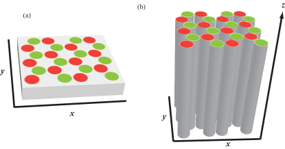
Figure S5: Sketch of photonic systems with underlying honeycomb structure: (a) Two-dimensional photonic crystal, (b) Photonic lattice.

In the main text, we applied this description to two different physical settings, a two-dimensional photonic crystal as in Fig. S5(a), or a photonic lattice of single-mode waveguides as in Fig. S5(b). Depending on the setting the modes $|a\rangle$, $|b\rangle$ can then be associated, e.g., to Wannier states which support the modes in a two-band approximation, or the wave-guide modes which are weakly coupled via tunneling. For the two-dimensional crystal the Hamiltonian is then interpreted as the generator of the time evolution in $t$, while for the photonic lattice it generates the propagation into the $z$ direction peleg ; makris . Accordingly, the eigenvalues $\varepsilon$ of $H$ determine the frequencies $\omega$ of quasibound states in the two dimensional crystal or the propagation constant $ck_{z}$ along the third direction in the photonic waveguide lattice. Eigenvalues with a positive imaginary part correspond to amplified states (in time or along the propagation direction, respectively), while those with a negative imaginary part correspond to decaying states. This interpretation can be made explicit when one focusses on a small window of the eigenvalue spectrum centered around a large value $\varepsilon_{0}$, which induces a rapid modulation $\exp(-is\varepsilon_{0})$ with $s=z$ or $t$. The underlying second-order wave equation (e.g., the Helmholtz equation or Maxwell’s equations) can then be simplified in a gradient expansion, which amounts to the substitution $-\partial_{s}^{2}\to(\varepsilon_{0}+i\partial_{s})^{2}\approx\varepsilon_{0}^{2}-2i\varepsilon_{0}\partial_{s}$. The first term is an offset which centers the spectrum around $\varepsilon_{0}$, so that the evolution equation for the $s$-dependent envelope function reads $i\partial_{s}\psi(x,y,s)=H\psi(x,y,s)$. For $s=z$, this is the paraxial approximation; and it is indeed this interpretation which has guided theory and experiment on $\mathcal{PT}$-symmetric peleg ; tachyons ; makris ; experiment1a ; experiment1b ; ramezani ; Regensburger ; talbot and strained Rechtsman photonic lattices.

References

- (1) F. Guinea, M. I. Katsnelson, and A. K. Geim, Nature Phys. 6, 30 (2010).
- (2) M. A. H. Vozmediano, M. I. Katsnelson and F. Guinea, Phys. Rep. 496, 109 (2010).
- (3) N. Levy, S. A. Burke, K. L. Meaker, M. Panlasigui, A. Zettl, F. Guinea, A. H. C. Neto, and M. F. Crommie, Science 329, 544 (2010).
- (4) H. Yan, Y. Sun, L. He, J.-C. Nie, and M. H. W. Chan, Phys. Rev. B 85, 035422 (2012).
- (5) R. Jackiw, Phys. Rev. D 29, 2375 (1984).
- (6) G. W. Semenoff, Phys. Rev. Lett. 53, 2449 (1984).
- (7) F. D. M. Haldane, Phys. Rev. Lett. 61, 2015 (1988).
- (8) O. Peleg, G. Bartal, B. Freedman, O. Manela, M. Segev, and D. N. Christodoulides, Phys. Rev. Lett 98, 103901 (2007).
- (9) S. Joannopoulos, J. D. Johnson, R. Meade, and J. Winn, Photonic Crystals. Molding the Flow of Light, 2nd ed. (Princeton University Press, Princeton, 2008).
- (10) S. Raghu and F. D. M. Haldane, Phys. Rev. A 78, 033834 (2008).
- (11) K. G. Makris, R. El-Ganainy, D. N. Christodoulides, and Z. H. Musslimani, Phys. Rev. Lett. 100, 103904 (2008).
- (12) A. Guo, G. J. Salamo, D. Duchesne, R. Morandotti, M. Volatier-Ravat, V. Aimez, G. A. Siviloglou, and D. N. Christodoulides, Phys. Rev. Lett. 103, 093902 (2009).
- (13) C. E. Rüter, K. G. Makris, R. El-Ganainy, D. N. Christodoulides, M. Segev, and D. Kip, Nature Phys. 6, 192 (2010).
- (14) A. Szameit, M. C. Rechtsman, O. Bahat-Treidel, and M. Segev, Phys. Rev. A 84, 021806(R) (2011).
- (15) H. Ramezani, T. Kottos, V. Kovanis, and D. N. Christodoulides, Phys. Rev. A 85, 013818 (2012).
- (16) A. Regensburger, C. Bersch, M.-A. Miri, G. Onishchukov, D. N. Christodoulides, and U. Peschel, Nature 488, 167 (2012).
- (17) C. M. Bender and S. Boettcher, Phys. Rev. Lett. 80, 5243 (1998).
- (18) P. R. Wallace, Phys. Rev. 71, 622 (1947).
- (19) K. Sasaki, Y. Kawazoe, and R. Saito, Prog. Theor. Phys. 113, 463 (2005).
- (20) K.-I. Sasaki and R. Saito, Prog. Theor. Phys. Suppl. 176, 253 (2008).
- (21) For details see the supplemental material.
- (22) H. Schomerus, Phys. Rev. Lett. 104, 233601 (2010); G. Yoo, H.-S. Sim, and H. Schomerus, Phys. Rev. A 84, 063833 (2011).
- (23) S. Longhi, Phys. Rev. A 82, 031801 (2010).
- (24) Y.D. Chong, L. Ge and A. D. Stone, Phys. Rev. Lett. 106, 093902 (2011).
- (25) M. -A. Miri, P. LiKamWa, and D. N. Christodoulides, Opt. Lett. 37, 764 (2012).
- (26) S. V. Iordanskii and A. E. Koshelev, JETP Lett. 41, 574 (1985).
- (27) D. Leykam, O. Bahat-Treidel, and A. S. Desyatnikov, Phys. Rev. A 86, 031805(R) (2012).
- (28) W. P. Su, J. R. Schrieffer, and A. J. Heeger, Phys. Rev. Lett. 42, 1698 (1979).
- (29) H. Schomerus, arXiv:1301.0777.
- (30) H. Ramezani, D. N. Christodoulides, V. Kovanis, I. Vitebskiy, and T. Kottos, Phys. Rev. Lett. 109, 033902 (2012).
- (31) M. C. Rechtsman, J. M. Zeuner, A. Tünnermann, S. Nolte, M. Segev, and A. Szameit, arXiv:1207.3596.