CERN-PH-TH/2012-313, DFPD 2012 TH-20, CP3-12-47
Lifting degeneracies in Higgs couplings using
single top production in association with a Higgs boson
Marco Farinaa, Christophe Grojeanb,c, Fabio Maltonid,
Ennio Salvionic,e and Andrea Thammc,f ***Email: mf627@cornell.edu, christophe.grojean@cern.ch, fabio.maltoni@uclouvain.be,
ennio.salvioni@cern.ch, andrea.thamm@cern.ch
(a) Department of Physics, LEPP, Cornell University, Ithaca, NY 14853, USA
(b) ICREA at IFAE, Universitat Autònoma de Barcelona, E-08193 Bellaterra, Spain
(c) Theory Division, Physics Department, CERN, CH-1211 Geneva 23, Switzerland
(d) Centre for Cosmology, Particle Physics and Phenomenology (CP3), Université Catholique de Louvain, Chemin du Cyclotron 2, B-1348 Louvain-la-Neuve, Belgium
(e) Dipartimento di Fisica e Astronomia, Università di Padova and INFN,
Via Marzolo 8, I-35131 Padova, Italy
(f) Institut de Théorie des Phénomènes Physiques, EPFL, CH-1015 Lausanne, Switzerland
Abstract
Current Higgs data show an ambiguity in the value of the Yukawa couplings to quarks and leptons. Not so much because of still large uncertainties in the measurements but as the result of several almost degenerate minima in the coupling profile likelihood function. To break these degeneracies, it is important to identify and measure processes where the Higgs coupling to fermions interferes with other coupling(s). The most prominent example, the decay of , is not sufficient to give a definitive answer. In this paper, we argue that -channel single top production in association with a Higgs boson, with , can provide the necessary information to lift the remaining degeneracy in the top Yukawa. Within the Standard Model, the total rate is highly reduced due to an almost perfect destructive interference in the hard process, . We first show that for non-standard couplings the cross section can be reliably computed without worrying about corrections from physics beyond the cutoff scale , and that it can be enhanced by more than one order of magnitude compared to the SM. We then study the signal with 3 and 4 ’s in the final state, and its main backgrounds at the LHC. We find the TeV run dataset to be sensitive to the sign of the anomalous top Yukawa coupling, while already a moderate integrated luminosity at TeV should lift the degeneracy completely.
1 Introduction
After 48 years of desperate searches, the most wanted elementary particle, the Higgs boson, or something that wickedly looks like it, has finally been caught by the ATLAS and CMS experiments [1, 2]. Uncertainties concerning its spin and CP properties remain and will be subject to intense experimental scrutiny in the present and forthcoming run of the LHC. Concurrently, an important program has been launched to measure its couplings to other known elementary particles of the Standard Model (SM). The goal is not so much to determine a few further unknown parameters of the SM but to understand the underlying structures of the laws of physics at high energy: if the SM were to be valid up to the scale of quantum gravity, the couplings of the Higgs boson would be uniquely fixed in terms of other already known and well-measured quantities. On the contrary, any deviation in these couplings, for instance of the order of 20%, would unambiguously signal new physics at a scale below 5 TeV.
The study of the LHC sensitivity to the Higgs couplings has been initiated in Refs. [3, 4, 5, 6]. Upon the first and still incomplete measurements reported by both ATLAS and CMS as well as by the Tevatron experiments, a simple methodology inspired by a chiral effective Lagrangian approach has been developed in Refs. [7, 8, 9] in order to quantify to which extent the Higgs boson is really fulfilling the role it has been devoted to in the SM, namely the screening of scattering amplitudes involving massive bosons and fermions at high energy.
At the LHC, the main production channel of the Higgs boson as well as its cleanest decay mode proceed through purely quantum mechanical processes and rely on couplings to massless gluons and photons that are vanishing in the Born approximation. This results in an ambiguity in the value of the tree-level Higgs couplings since the coupling likelihood function exhibits several and almost degenerate minima (see e.g. Refs. [6, 8, 9]). It has been emphasized [9, 10] that these degeneracies are likely to remain even after the on-going analyses will be extended to the whole 8 TeV dataset. Measuring processes involving real top quarks in the final state will bring invaluable information. With the largest rate, the Higgs production in association with a top pair is a golden channel and has received great attention by the experimental [11, 12] as well as theoretical [13, 14, 15, 16, 17] communities.
In this paper we argue that, even though subleading, Higgs boson production in association with a single top quark can also bring valuable information, in particular regarding the sign of the top Yukawa coupling111The sign of the top Yukawa coupling is not physical by itself, but the relative sign compared to the Higgs coupling to gauge bosons (we take the latter to be positive) is physical.. This is because an almost totally destructive interference between two large contributions, one where the Higgs couples to a space-like boson and the other where it couples to the top quark, takes place in the SM. This fact can be exploited to probe deviations in the Higgs coupling structure, which will inevitably jeopardize perturbative unitarity at high energy and lead to a striking enhancement of the cross section compared to the SM. We discuss how this enhancement can be used to extract information on the sign of the top Yukawa coupling and we show that production can be used to lift the degeneracy plaguing the Higgs coupling fit of the LHC data. While a moderate integrated luminosity at TeV should allow us to make a conclusive statement, we point out that already with the full 2012 luminosity, corresponding to per experiment, an interesting sensitivity on the sign of the top Yukawa could be reached.
In our study we focus on the decay of the Higgs into , updating the early analysis of Ref. [18] (see also Refs. [19, 20]). This choice leads to an experimental signature (lepton + missing energy + multijets, among which are -jets) which is very similar to the one ATLAS and CMS have already analyzed in their searches for production [11, 12]. In this respect we believe that the experimental collaborations could easily perform the analysis we propose here in the very near future, thus adding new important information to the challenge of identifying the true nature of the recently discovered particle.
The large enhancement of the cross section for nonstandard Higgs couplings is associated to the growth of the scattering amplitude at high energy, which in turn implies that perturbative unitarity is lost at some UV scale . We estimate , which acts as the cutoff of our effective theory, to be at least of TeV and thus above the energy scales that the LHC will be able to probe. In fact, the invariant mass distribution in LHC collisions essentially vanishes above 1 TeV, therefore we can safely conclude that our analysis remains insensitive to UV physics above the cutoff scale.
Our paper is structured as follows: we start by introducing the general features of the process and discussing its implications, including an estimate of the scale where perturbative unitarity is lost, in Section 2. We proceed in Section 3 to the analysis of the signal and of the main backgrounds at the LHC, performing a parton-level simulation. In Section 4, we discuss the implications on the determination of the Higgs parameters. Finally, we conclude in Section 5. Unless otherwise specified, the Higgs mass is assumed to be throughout this work. For the top mass we take . Finally, the shorthand is always understood to include also the charge-conjugated case where is replaced by . Therefore all our cross sections include both and production.
2 Single top and Higgs associated production
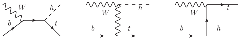
The Feynman diagrams contributing to the core process are shown in Fig. 1. The diagram where the Higgs is emitted from a leg is suppressed by the bottom Yukawa, and will be consistently neglected in our study. In the production process at the LHC the initial is radiated from a quark in the proton, and is thus spacelike. However, at high energy the effective approximation [21, 22] holds, which allows us to factorize the process into the emission of an approximately on-shell from the quark times its hard scattering with a bottom. Thus it makes sense to discuss the amplitude for at high energies assuming the initial to be on-shell, in order to gain an approximate understanding of the full picture.
In the high-energy, hard-scattering regime, where , the amplitude for (the longitudinal polarization dominates at large ) reads222We take final momenta outgoing, and define , . is the azimuthal angle around the axis, which is taken parallel to the direction of motion of the incoming .
| (2.1) |
where we have omitted terms that vanish in the high-energy limit and, for simplicity, also neglected the Higgs mass in addition to setting . The generalized couplings of the Higgs are defined as and . The functions are given by
| (2.2) | ||||
| (2.3) |
where in the rightmost term of each line we have chosen a specific basis for the spinors, namely
| (2.4) |
which correspond to the chiral states () in the limit333However, note that the limit does not interest us here.. The amplitudes involving the helicity state , which is identified with a right-handed bottom since we are assuming , exactly vanish due to the structure of the couplings of the to fermions. From Eq. (2.1) we see that when the amplitude grows with energy like and is enhanced compared to the case (which includes the SM), where the amplitude is constant in the large limit. The non-cancellation of the terms in the amplitude growing with energy is at the origin of the striking enhancement of the cross section when .
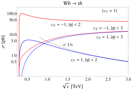
The cross section for is shown as a function of the center of mass energy in Fig. 2. The large enhancement of the hard scattering cross section (defined by a centrality cut ) for is evident.444Incidentally, we note that the cross section shows another feature, a Coulomb enhancement at small due to the diagram with a exchange in the -channel. As can be read off Fig. 2 the forward cross section tends to a constant limit for large , which can be computed in a simple way in terms of the parameter alone and is insensitive to the value of . A short discussion of the forward cross section is contained in Appendix A. At large energies, the amplitude is constant for and thus the cross section vanishes as . On the other hand, when the amplitude grows with energy like and as a consequence the cross section tends to a constant for large . It is easy to compute this asymptotic value of the cross section: squaring the leading term of the amplitude in Eq. (2.1), summing and averaging over polarizations and integrating over we find
| (2.5) |
This simple formula gives accurate results: for example for , and a centrality cut555Note that for the expression in Eq. (2.5) to be reliable, cannot be too large. In fact, as already mentioned, in the forward region the cross section has a Coulomb enhancement which is not captured by the approximations we made here. See also Appendix A. we find that the cross section computed without any approximations is , whereas .
Since for the hard scattering amplitude grows with energy, perturbative unitarity will be lost at some cutoff scale , which we now estimate. In the spinor basis of Eq. (2.4), only one -wave amplitude is non-vanishing
| (2.6) |
from which, imposing the condition , we find that perturbative unitarity is violated at a scale with
| (2.7) |
For example, for the cutoff is . One may worry about other processes involving top quarks, in which perturbative unitarity could be lost at a scale lower than the one in Eq. (2.7) for . A relevant and often mentioned process is , for which we find For this formula yields , essentially the same cutoff scale we found for . For previous discussions of perturbative unitarity breakdown in processes with external fermions, see Refs. [23, 24].
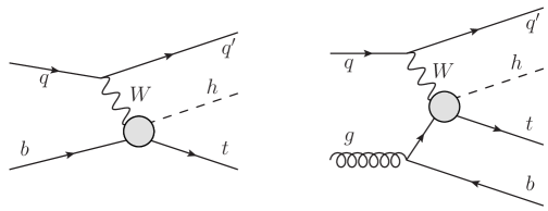
Having analyzed the behavior of the partonic cross section, we can now turn our attention to single top and Higgs associated production in hadron collisions. At the LHC, -channel single top production goes through an initial-state gluon splitting into a pair. Such a process can be efficiently described by a -flavor scheme where ’s are in the initial state and described by a perturbative PDF, Fig. 3(a). In this scheme, the non-collinearly enhanced contribution, where the spectator (i.e. the one not struck by the boson) is central and at high (see Fig. 3(b)), is moved to the next-to-leading order term. This contribution, which we indicate with , is finite and can be easily calculated at tree-level, contributing to a final state signature with an extra -jet, a useful handle to suppress the background. In Table 1 we present the rates for production in the -flavor scheme, fully inclusive as well as with the requirement of the extra to be in the tagging region, for and TeV, in the cases. Our analysis in Section 3 will consider both processes, which lead to final states containing and -jets respectively, once the decay of the Higgs to is taken into account. The cross sections in Table 1 were computed using MadGraph 5[25] with CTEQ6L1 PDFs [26], setting the factorization and renormalization scales to the default event-by-event MadGraph 5 value. As an estimate of the theoretical uncertainty on the signal, we have computed the fully inclusive cross sections at NLO in QCD, in the -flavor scheme, using aMC@NLO [27, 28, 29] and CTEQ6M PDFs [26]. The results are reported in Table 2, where the uncertainties correspond to variations of the factorization and renormalization scales with around from to . The NLO cross sections appear to be extremely stable under radiative corrections and therefore we deem the theory uncertainty of the signal rates in our analysis negligible.
| TeV | ||||
|---|---|---|---|---|
| TeV | ||||
| TeV | ||
|---|---|---|
| TeV | ||
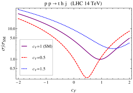
The striking enhancement of the hadronic cross section for is shown in Fig. 4, where for an LHC energy of , normalized to its SM value, is displayed as a function of for three different choices of (very similar plots are obtained considering and/or the process). For example, for a standard coupling, i.e. , a top Yukawa with equal magnitude and opposite sign with respect to the standard one () yields an enhancement of the cross section of more than a factor 10.
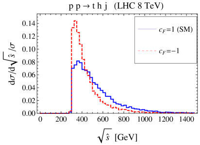
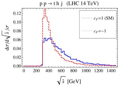
As noted above, perturbative unitarity in scattering is lost at a scale for . Figure 5 clearly shows that after convolution with the PDFs the contribution of the region , where is the center of mass energy of the system, to the hadronic cross section is negligible. This implies that our perturbative computations can be fully trusted. Indeed Fig. 5 demonstrates that the relative contribution to the cross section from large values of is more sizable in the SM than for . This is compatible with the different behaviors of the partonic cross section in the two cases, shown in Fig. 2.
3 Signal and background study
3.1 Parton-level simulation
Signal and background events have been generated at the parton level using MadGraph 5 with CTEQ6L1 PDFs, setting the factorization and renormalization scales to the default event-by-event MadGraph 5 value. Jets are defined at the parton level. In order to take showering, hadronization, detector and reconstruction effects minimally into account, we smear the of the jets uniformly in using a jet energy resolution defined by
| (3.1) |
where the parameters are taken to be , and . With these choices, Eq. (3.1) is compatible with the results of the ATLAS jet energy resolution study of Ref. [30] (see Fig. 9 there). The jet 4-momentum is then rescaled by a factor . The acceptance cuts reported in Table 3, chosen following the ATLAS analysis [11], are applied on the physical objects. We do not require any acceptance cut on the missing transverse energy.
| Cut | ||||||
|---|---|---|---|---|---|---|
| Value | GeV | GeV | GeV |
An object is considered to be missed if it does not pass one of the acceptance cuts. If, in particular, two jets are collinear with we merge them by summing their 4-momenta and we consider them as a single jet when applying further cuts.666The exception to this procedure is the case where the coming from a semileptonic top decay is collinear to another jet. Since we are assuming ideal semileptonic top reconstruction (see below), we simply reject the event in this case. Additionally we require the lepton to be isolated from any jet in the event, including those that do not pass acceptance cuts and therefore are missed.
In all the signal and background processes we consider in this paper, a semileptonically decaying top is present. We assume a efficiency for the reconstruction of this top, which implies an unambiguous identification of the originating from its decay. This assumption is of course idealized, however the use of a more realistic semileptonic top reconstruction efficiency will only affect the overall normalization of both signal and background, and not their relative values.
Concerning -tagging, we assume the following performance: efficiency , charm mistag probability and light jet mistag probability [11]. Finally we assume a lepton reconstruction efficiency .
3.2 Final state with -tags
We start by discussing the 3 -jet final state, which arises from after selecting the Higgs decay into . Requiring the top to decay semileptonically () gives the signature
| (3.2) |
We can now turn our attention to the most relevant backgrounds:777For the sake of readability we do not write the top decay explicitly, as it is the same for all processes.
-
•
, : an irreducible background where a boson mimics the Higgs in decaying to .
-
•
: an irreducible QCD background.
-
•
, : a reducible background where either the or are mis-tagged.
-
•
, : also in this case, either the or are mis-tagged while the other is missed.
As can be seen in Table 4 for 8 TeV and in Table 5 for 14 TeV, after acceptance cuts and efficiencies the last two backgrounds are extremely large. In particular, their values are larger than those quoted in Ref. [18], mainly due to a larger charm mistag rate considered here (we use , whereas Ref. [18] adopted ) and to the fact that we increased the threshold for jets, which results in a larger probability of missing a jet from . The dominance of backgrounds where a is mistagged suggests that it may be sensible to prefer a -tagging performance with smaller efficiency but higher rejection against charm. However, for definiteness we stick to the numbers reported in Section 3.1, taken from Ref. [11].
After acceptance cuts and efficiencies, the signal is overwhelmed by the background not only for the standard case , but even considering the enhanced case (we set ). Thus, we require a set of additional cuts in order to isolate the signal. These cuts are listed in Tables 4-5, together with the cross sections obtained after their application. The value of each cut is chosen by optimizing the Poisson exclusion limit in the case. We remark that since we are assuming ideal top reconstruction, the coming from the semileptonic top is always assumed to be unambiguously identified, therefore no cut on it is applied beyond the detector ones, neither for the signal nor for the backgrounds.
The first cut we apply requires the pair to have an invariant mass around , which of course helps to eliminate the background. The second cut selects large values for the invariant mass and is effective against the reducible backgrounds, in particular it suppresses enormously , where the jet and 2 ’s are decay products of a top and therefore we expect their invariant mass to be close to . The last cut singles out a forward jet, which is a distinctive feature of the signal. However, after all cuts the background cross section, completely dominated by , is still one order of magnitude larger than the signal for .
| Signal | Backgrounds | ||||||
|---|---|---|---|---|---|---|---|
| Cuts | Total | ||||||
| Acceptance Cuts + | |||||||
| GeV | |||||||
| GeV | |||||||
| Events at | |||||||
| Signal | Backgrounds | ||||||
|---|---|---|---|---|---|---|---|
| Cuts | Total | ||||||
| Acceptance Cuts + | |||||||
| GeV | |||||||
| GeV | |||||||
| Events at | |||||||
In the last line of Tables 4 and 5, we present the number of signal and total background events expected after of integrated luminosity. At 8 TeV, the Poisson exclusion is at CL or (by abuse of notation, we are expressing the probability in terms of number of ’s, e.g. approximately corresponds to the CL), while at TeV it reaches .
3.3 Final state with -tags
As suggested in Ref. [18], a way to enhance the sensitivity on the signal is to require an extra , coming from the splitting of an initial gluon: the process of interest is thus . Requiring a semileptonic top and the decay leads to the signature
| (3.3) |
Here the main backgrounds are:
-
•
, : an irreducible background where the mimics the Higgs.
-
•
: similarly to the case, an irreducible QCD background.
-
•
, : a reducible background where one of the two jets, originating from a hadronically decaying , is missed.
-
•
, (one mistag): here the or the is mis-tagged, while either the other one is missed (and one is not tagged) or one of the ’s is missed.
-
•
, (two mistags): in this case both and are mistagged.
Looking at Tables 6 and 7, we see that requiring 4 -jets allows us to obtain a much larger signal to background ratio after acceptance cuts compared to the case. On the other hand, the overall rates are obviously smaller. Analogously to what was done in the case, a set of additional cuts are imposed to enhance the signal. The cuts are listed in Tables 6-7, together with the cross sections obtained after their application. The value of each cut is again chosen by optimizing the Poisson exclusion limit in the case.
The first cut requires the invariant mass of one of the 3 pairs (we recall that ideal reconstruction of the semileptonic top is assumed) to be inside a window around . This helps again to eliminate the background. The second cut demands all invariant masses to be higher than about , and is most effective on , where the mis-tagged and , coming from a decay, have an invariant mass around . The last cut requires all 3 pairs to have a large invariant mass. This efficiently suppresses the backgrounds, for which in most cases at least one pair comes from a top decay and thus has an invariant mass .
| Signal | Backgrounds | |||||||
|---|---|---|---|---|---|---|---|---|
| Cuts | Total | (mis) | ||||||
| Acceptance Cuts + | ||||||||
| GeV | ||||||||
| min GeV | ||||||||
| min GeV | ||||||||
| Events at | ||||||||
| Signal | Backgrounds | |||||||
|---|---|---|---|---|---|---|---|---|
| Cuts | Total | (mis) | ||||||
| Acceptance Cuts + | ||||||||
| GeV | ||||||||
| min GeV | ||||||||
| min GeV | ||||||||
| Events at | ||||||||
The exclusion limits obtained for , assuming of data, are and at 8 and 14 TeV respectively. The sensitivity at 8 TeV is comparable to the one obtained in the case, while at 14 TeV requiring an extra -jet improves the result significantly.
Before discussing the implications of our results, we wish to comment here on the sensitivity of the proposed analysis to the process. As can be read from Tables 6 and 7, this process makes up a sizable fraction of the cross section after the cuts. Moreover, after the first three cuts, the rate for is comparable to the signal for . Being insensitive to the sign of the top Yukawa, can be considered as a background process in our analysis. It is, however, quite useful to observe that the simple search strategy we propose in the channel would be sensitive to both single and pair top production in association with a Higgs boson. In this respect, a key role is played by the cut on that was designed to suppress processes with a pair in the final state, as discussed above. The relative contribution of to the background with one mistag, on the other hand, is small, approximately .
4 Implications on Higgs couplings
We are now able to study the implications of our results on the general parameter space of Higgs couplings. To do so we combine the two analyses that we discussed in Section 3, i.e. and -tags, to exploit the full LHC sensitivity in production. Note that in the combination we consider the and samples as independent. While this is an approximation (which can be easily lifted in a more realistic analysis by defining fully exclusive samples), in practice it has a small effect as the sample is significantly smaller than the one. We combine the (Poisson) -values through Fisher’s method, defining
| (4.1) |
where in our case, and are the -values of the two analyses. It can be shown that has a distribution with degrees of freedom. Thus the combined -value is the one associated to the value of at each point in parameter space. This definition is conservative compared to estimate based on the naive product of -values.
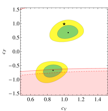
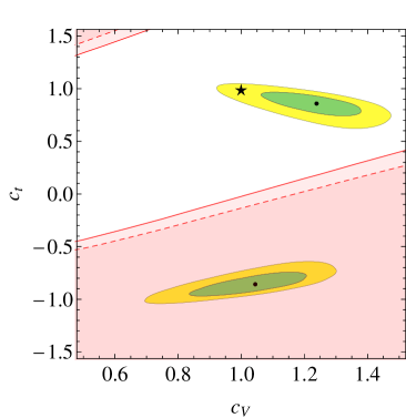
In Fig. 6 we present the results of our analysis in the plane, where a universal rescaling of the Higgs couplings to fermions is assumed. The regions that can be excluded (at CL) by production with an integrated luminosity of and are presented, along with the regions currently favored by a fit to Higgs data. As can be seen, already at TeV parts of the preferred region with can be excluded. The current best fit point with is excluded at with . On the other hand, a moderate luminosity at TeV can conclusively remove the degeneracy between the two regions that are at the present time preferred by Higgs data, for example reaching a exclusion of the best fit point with after . Notice that in addition to the production cross section (recall Fig. 4), also the branching ratio of the Higgs into depends on the parameters .
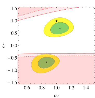
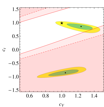
It is also possible to relax the assumption of universal couplings of the Higgs to fermions and consider the case where only the coupling has a rescaled value compared to the SM while , so in particular is equal to its SM value. In this case, the rate is essentially fixed by the dependence on of the production cross section (a mild sensitivity to through the Higgs total width is also present). The results are shown in the plane in Fig. 7. Excluded regions at 95% C.L. are displayed for fb-1 and fb-1 integrated luminosity. Superimposed are the regions currently favored by Higgs data. The most striking feature is, that the best fit region with can already be completely excluded at TeV with fb-1 (reaching a exclusion of the best fit point with negative ).
5 Conclusions
After the time of discovery comes the need for measuring. The couplings of the putative Higgs boson are of prime importance since they control the behavior of the whole theory at high energy. The dominant processes involving the Higgs boson that are currently investigated at the LHC do not allow us to determine all its couplings unambiguously. An important task now is therefore to systematically identify additional processes that could complement the first LHC information and lift degeneracies appearing in Higgs coupling fits.
In this paper, we have studied single top production in association with a Higgs boson, focusing on the Higgs decay into . We discussed the form of the amplitude of the hard scattering process , showing that for nonstandard couplings of the Higgs to the boson and/or to the top quark a striking enhancement of the cross section can be obtained. The enhancement is due to the non-cancellation of terms that grow with energy in the amplitude and lead to violation of perturbative unitarity at some UV scale. We estimate the cutoff scale to be at least , concluding that corrections to our computation of the cross section from physics above the cutoff are always negligible.
We have performed a parton-level study of the LHC signal processes and , and of the corresponding irreducible and some of the most relevant reducible backgrounds. The combination of the two final states, containing and -jets respectively, shows that if a universal rescaling of the fermion couplings is assumed, already at TeV parts of the preferred region with can be excluded. On the other hand, a moderate luminosity of at TeV can conclusively remove the degeneracy between the two regions that are at the present time preferred by Higgs data, reaching a exclusion of the best fit point with negative . In addition, we investigated the case where only the coupling differs from its SM value while the other Yukawa couplings are standard. Here, the best fit region with negative top Yukawa coupling can be completely excluded at TeV with fb-1, reaching a exclusion of the best fit point with .
Our results therefore motivate the undertaking of a full-fledged analysis by the ATLAS and CMS collaborations on one side, and the improvement on the accuracy of the theoretical predictions on the other. In the former case, in addition to having a complete simulation of events, one could also study the possibility of improving the signal over background ratio by using further discriminating variables (such as for example the different rates for and with respect to the main backgrounds which are symmetric) or multivariate analyses. On the latter, it would be certainly interesting to evaluate the (possibly significant) impact of NLO QCD corrections to signal and irreducible backgrounds, i.e., and , a task that can now be accomplished in a fully automatic way [28, 27, 15, 32].
Further information on the Higgs couplings to heavy quarks could also come from other processes at the LHC. One example is double Higgs production, . This process proceeds through a triangle and a box diagram, which, again, interfere destructively in the SM and therefore result in a sensitive probe of the Higgs-heavy quarks interactions, see, e.g., Refs. [33, 34, 35]. Finally we remark that complementary information could a priori also come from the observation of very recently reported by LHC [36]. The measured value of BR agrees well with the SM prediction [37]. The SM contribution is actually dominated by the interactions associated to the top Yukawa coupling and therefore this measurement could be naively expected to provide a good probe of any deviation of the top Yukawa itself. However, only the Yukawa interactions between the Goldstone bosons and the quarks contribute to this process. What we have proposed to probe via production is rather the interaction of the physical Higgs boson with the top quark, i.e. the one controlled by the parameter . Actually, if the deviations from originate from pure Higgs non-linearities as in composite Higgs models, for instance via a higher dimensional operator like , then it is easy to see that the prediction for BR remains unaffected.888We thank G. Isidori for illuminating discussions on this point.
Note added
During the final stages of this project another study discussing production appeared [38] that focuses on the decay channel.
Acknowledgments
We are grateful to A. Coccaro, P. Francavilla, G. Isidori and V. Sanz for useful discussions. We also wish to thank V. Hirschi for help with aMC@NLO. M.F. thanks CERN for hospitality during the early stages of this work. This research has been partly supported by the European Commission under the ERC Advanced Grant 226371 MassTeV and the contract PITN-GA-2009-237920 UNILHC. C.G. is also supported by the Spanish Ministry MICNN under contract FPA2010-17747. The work of F.M. is partially supported by the IAP Program, BELSPO VII/37 and the IISN-FNRS conventions 4.4511.10 and 4.4517.08. E.S. has been supported in part by the European Commission under the ERC Advanced Grant 267985 DaMeSyFla. The work of M.F. has been supported in part by the NSF grant PHY-0757868 and by the Fondazione A. Della Riccia. A.T. has been partially supported by the Swiss National Science Foundation under contract 200020-138131.
Appendix A Forward scattering
The forward cross section for the partonic process , defined for example by a cut on , can be computed for large in a very simple way. In fact, for this purpose the diagram with top exchange in the -channel can be neglected, and we only need to look at the diagram with exchange in the -channel. In the regime we are interested in, i.e. large , the longitudinal polarization of the dominates. The leading term in the amplitude, which is enhanced at small , goes as and reads
| (A.1) |
At large and generic , the fermion bilinears relevant to the amplitude read
| (A.2) | ||||
| (A.3) |
where the functions have been defined in Eqs. (2.2-2.3), and the dots stand for subleading terms. Thus squaring the amplitude in Eq. (A.1), summing and averaging over polarizations (we neglect the contributions of the transverse components of the ) and recalling that we are interested in the region we find
| (A.4) |
from which we derive the approximate expression of the forward cross section
| (A.5) |
valid for (i.e. for large ). We note that as expected, the forward cross section is controlled only by and is insensitive to the value of . As a consequence, the forward cross section is insensitive to the growth with energy of the “hard scattering” amplitude, which takes place for and was discussed in Sec. 2. As a numerical example, let us consider , a cut and let us set the center of mass energy to . Then computing the cross section without approximations gives
| (A.6) |
whereas using the approximate formula in (A.5) yields , a very accurate result. The factor has the value .
References
- [1] ATLAS Collaboration, Phys. Lett. B 716 (2012) 1 [arXiv:1207.7214 [hep-ex]].
- [2] CMS Collaboration, Phys. Lett. B 716 (2012) 30 [arXiv:1207.7235 [hep-ex]].
- [3] D. Zeppenfeld, R. Kinnunen, A. Nikitenko and E. Richter-Was, Phys. Rev. D 62 (2000) 013009 [arXiv:hep-ph/0002036].
- [4] M. Dührssen, ATL-PHYS-2003-030 [http://cdsweb.cern.ch/record/685538].
- [5] M. Dührssen, S. Heinemeyer, H. Logan, D. Rainwater, G. Weiglein and D. Zeppenfeld, Phys. Rev. D 70 (2004) 113009 [arXiv:hep-ph/0406323].
- [6] R. Lafaye, T. Plehn, M. Rauch, D. Zerwas and M. Dührssen, JHEP 0908 (2009) 009 [arXiv:0904.3866 [hep-ph]].
- [7] D. Carmi, A. Falkowski, E. Kuflik and T. Volansky, JHEP 1207 (2012) 136 [arXiv:1202.3144 [hep-ph]].
- [8] A. Azatov, R. Contino and J. Galloway, JHEP 1204 (2012) 127 [arXiv:1202.3415 [hep-ph]].
- [9] J. R. Espinosa, C. Grojean, M. Mühlleitner and M. Trott, JHEP 1205 (2012) 097 [arXiv:1202.3697 [hep-ph]].
- [10] A. Azatov, R. Contino, D. Del Re, J. Galloway, M. Grassi and S. Rahatlou, JHEP 1206 (2012) 134 [arXiv:1204.4817 [hep-ph]].
-
[11]
ATLAS Collaboration,
ATLAS-CONF-2012-135, September 2012
[http://cdsweb.cern.ch/record/1478423]. -
[12]
CMS Collaboration,
CMS-PAS-HIG-12-025, September 2012
[http://cdsweb.cern.ch/record/1460423]. - [13] W. Beenakker, S. Dittmaier, M. Kramer, B. Plumper, M. Spira and P. M. Zerwas, Phys. Rev. Lett. 87 (2001) 201805 [arXiv:hep-ph/0107081].
- [14] S. Dawson, L. H. Orr, L. Reina and D. Wackeroth, Phys. Rev. D 67 (2003) 071503 [arXiv:hep-ph/0211438].
- [15] R. Frederix, S. Frixione, V. Hirschi, F. Maltoni, R. Pittau and P. Torrielli, Phys. Lett. B 701 (2011) 427 [arXiv:1104.5613 [hep-ph]].
- [16] M. V. Garzelli, A. Kardos, C. G. Papadopoulos and Z. Trocsanyi, Europhys. Lett. 96 (2011) 11001 [arXiv:1108.0387 [hep-ph]].
- [17] C. Degrande, J. M. Gerard, C. Grojean, F. Maltoni and G. Servant, JHEP 1207 (2012) 036 [arXiv:1205.1065 [hep-ph]].
- [18] F. Maltoni, K. Paul, T. Stelzer and S. Willenbrock, Phys. Rev. D 64, 094023 (2001) [arXiv:hep-ph/0106293].
- [19] T. M. P. Tait and C. -P. Yuan, Phys. Rev. D 63, 014018 (2000) [arXiv:hep-ph/0007298].
- [20] V. Barger, M. McCaskey and G. Shaughnessy, Phys. Rev. D 81, 034020 (2010) [arXiv:0911.1556 [hep-ph]].
- [21] S. Dawson, Nucl. Phys. B 249 (1985) 42.
- [22] G. L. Kane, W. W. Repko and W. B. Rolnick, Phys. Lett. B 148 (1984) 367.
- [23] T. Appelquist and M. S. Chanowitz, Phys. Rev. Lett. 59 (1987) 2405 [Erratum-ibid. 60 (1988) 1589].
- [24] F. Maltoni, J. M. Niczyporuk and S. Willenbrock, Phys. Rev. D 65 (2002) 033004 [arXiv:hep-ph/0106281].
- [25] J. Alwall, M. Herquet, F. Maltoni, O. Mattelaer and T. Stelzer, JHEP 1106, 128 (2011) [arXiv:1106.0522 [hep-ph]].
- [26] J. Pumplin, D. R. Stump, J. Huston, H. L. Lai, P. M. Nadolsky and W. K. Tung, JHEP 0207, 012 (2002) [arXiv:hep-ph/0201195].
- [27] R. Frederix, S. Frixione, F. Maltoni and T. Stelzer, JHEP 0910 (2009) 003 [arXiv:0908.4272 [hep-ph]].
- [28] V. Hirschi, R. Frederix, S. Frixione, M. V. Garzelli, F. Maltoni and R. Pittau, JHEP 1105 (2011) 044 [arXiv:1103.0621 [hep-ph]].
- [29] http://amcatnlo.cern.ch .
- [30] ATLAS Collaboration, arXiv:1210.6210 [hep-ex].
- [31] J. R. Espinosa, C. Grojean, M. Mühlleitner and M. Trott, JHEP 1212 (2012) 045 [arXiv:1207.1717 [hep-ph]].
- [32] R. Frederix, E. Re and P. Torrielli, JHEP 1209 (2012) 130 [arXiv:1207.5391 [hep-ph]].
- [33] R. Gröber and M. Mühlleitner, JHEP 1106 (2011) 020 [arXiv:1012.1562 [hep-ph]].
- [34] R. Contino, M. Ghezzi, M. Moretti, G. Panico, F. Piccinini and A. Wulzer, JHEP 1208 (2012) 154 [arXiv:1205.5444 [hep-ph]].
- [35] M. Gillioz, R. Gröber, C. Grojean, M. Mühlleitner and E. Salvioni, JHEP 1210 (2012) 004 [arXiv:1206.7120 [hep-ph]].
- [36] LHC Collaboration, Phys. Rev. Lett. 110 (2013) 021801 [arXiv:1211.2674 [hep-ex]].
- [37] A. J. Buras, J. Girrbach, D. Guadagnoli and G. Isidori, Eur. Phys. J. C 72 (2012) 2172 [arXiv:1208.0934 [hep-ph]].
- [38] S. Biswas, E. Gabrielli and B. Mele, JHEP 1301 (2013) 088 [arXiv:1211.0499 [hep-ph]].