Flavor Violating Higgs Decays
Abstract
We study a class of nonstandard interactions of the newly discovered 125 GeV Higgs-like resonance that are especially interesting probes of new physics: flavor violating Higgs couplings to leptons and quarks. These interaction can arise in many frameworks of new physics at the electroweak scale such as two Higgs doublet models, extra dimensions, or models of compositeness. We rederive constraints on flavor violating Higgs couplings using data on rare decays, electric and magnetic dipole moments, and meson oscillations. We confirm that flavor violating Higgs boson decays to leptons can be sizeable with, e.g., and branching ratios of perfectly allowed by low energy constraints. We estimate the current LHC limits on and decays by recasting existing searches for the SM Higgs in the channel and find that these bounds are already stronger than those from rare tau decays. We also show that these limits can be improved significantly with dedicated searches and we outline a possible search strategy. Flavor violating Higgs decays therefore present an opportunity for discovery of new physics which in some cases may be easier to access experimentally than flavor conserving deviations from the Standard Model Higgs framework.
pacs:
FERMILAB-PUB-12-498-T
I Introduction
Both ATLAS and CMS have recently announced the discovery of a Higgs-like resonance with a mass of GeV [1, 2, 3, 4], further supported by combined Tevatron data [5]. An interesting question is whether the properties of this resonance are consistent with the Standard Model (SM) Higgs boson. Deviations from the SM predictions could point to the existence of a secondary mechanism of electroweak symmetry breaking or to other types of new physics not too far above the electroweak scale. While there is a large ongoing experimental effort to measure precisely the decay rates into the channels that dominate for the SM Higgs, it is equally important to search for Higgs decays into channels that are subdominant or absent in the SM. For instance, since the couplings of the Higgs boson to quarks of the first two generations and to leptons are suppressed by small Yukawa couplings in the SM, new physics contributions can easily dominate over the SM predictions. Another possibility, and the main topic of this paper, is flavor violating (FV) Higgs decays, for instance into or final states. The study of FV couplings of the Higgs boson has a long history [6, 7, 8, 9, 10, 11, 12, 13, 14, 15, 16, 17, 18, 19, 20, 21, 22, 23, 24, 25, 26]. In this paper, we refine the indirect bounds on the FV couplings. Most importantly, we discuss in detail possible search strategies for FV Higgs decays at the LHC and derive for the first time limits from LHC data.
As pointed out in the previous literature, and confirmed by the present analysis, the indirect constraints on many FV Higgs decays are rather weak. In particular, the branching ratios for and can reach up to 10% [24]. In fact, for and already now111By we always mean the sum of and and similarly for the other decay modes., without targeted searches, the LHC is placing limits that are comparable to or even stronger than those from rare decays. As we shall see later, re-casting a analysis with 4.7 fb-1 of 7 TeV ATLAS data [27] gives a bound on the branching fraction of the Higgs into or around 10%. We will also demonstrate that dedicated searches can be much more sensitive.
These decays could thus give a striking signature of new physics at the LHC, and we strongly encourage our experimental colleagues to include them in their searches. Another experimentally interesting set of decay channels are flavor conserving decays to the first two generations, e.g., , on which we will comment further below. We emphasize that large deviations from the SM do not require very exotic flavor structures. A branching ratio for comparable to the one for , or a branching ratio a few times larger than in the SM can arise in many models of flavor (for instance in models with continuous and/or discrete flavor symmetries [28], or in Randall-Sundrum models [29]) as long as there is new physics at the electroweak scale and not just the SM. The lepton flavor violating decay has been studied in [11], and it was found that the branching ratio for this decay can be up to 10% in certain Two Higgs Doublet Models (2HDMs).
In fact, there may already be experimental hints that the Higgs couplings to fermions may not be SM-like. For instance, the BaBar collaboration recently announced a indication of flavor universality violation in transitions [30], which can be explained for instance by an extended Higgs sector with nontrivial flavor structure [31].
The paper is organized as follows. In Sec. II we introduce the theoretical framework we will use to parameterize the flavor violating decays of the Higgs. In Sec. III we derive bounds on flavor violating Higgs couplings to leptons and translate these bounds into limits on the Higgs decay branching fractions to the various flavor violating final states. In Sec. IV we do the same for flavor violating couplings to quarks. We shall see that decays of the Higgs to and to with sizeable branching fractions are allowed, and that also flavor violating couplings of the Higgs to top quarks are only weakly constrained. Motivated by this we turn to the LHC in Section V and estimate the current bounds on Higgs decays to and using data from an existing search. We also discuss a strategy for a dedicated search and comment on differences with the SM searches. We will see that the LHC can make significant further progress in probing the Higgs’ flavor violating parameters space with existing data. We conclude in Section VI. In the appendices, we give more details on the calculation of constraints from low-energy observables.
II The framework
After electroweak symmetry breaking (EWSB) the fermionic mass terms and the couplings of the Higgs boson to fermion pairs in the mass basis are in general
| (1) |
where ellipses denote nonrenormalizable couplings involving more than one Higgs field operator. In our notation, are doublets, the weak singlets, and indices run over generations and fermion flavors (quarks and leptons) with summation implicitly understood. In the SM the Higgs couplings are diagonal, , but in general NP models the structure of the can be very different. Note that we use the normalization GeV here. The goal of the paper is to set bounds on and identify interesting channels for Higgs decays at the LHC. Throughout we will assume that the Higgs is the only additional degree of freedom with mass and that the ’s are the only source of flavor violation. These assumptions are not necessarily valid in general, but will be a good approximation in many important classes of new physics frameworks. Let us now show how can arise in two qualitatively different categories of NP models.
A single Higgs theory.
Let us first explore the possibility that the Higgs is the only field that causes EWSB (see also [15, 23, 19, 32, 33, 34, 10]). For simplicity let us also assume that at energies below GeV the spectrum consists solely of the SM particles: three generations of quarks and leptons, the SM gauge bosons and the Higgs at 125 GeV. Additional heavy fields (e.g. scalar or fermionic partners which address the hierarchy problem) can be integrated out, so that we can work in effective field theory (EFT)—the effective Standard Model. In addition to the SM Lagrangian
| (2) | ||||
there are then also higher dimensional terms due to the heavy degrees of freedom that were integrated out:
| (3) |
Here we have written out explicitly only the terms that modify the Yukawa interactions. We can truncate the expansion after the terms of dimension 6, since these already suffice to completely decouple the values of the fermion masses from the values of fermion couplings to the Higgs boson. Additional dimension 6 operators involving derivatives include
| (4) | ||||
where . The couplings are complex in general, while the are real. The derivative couplings do not give rise to fermion-fermion-Higgs couplings after EWSB and are irrelevant for our analysis. In Eq. (4) there are in principle also terms of the form , which, however, can be shown to be equivalent to (3) by using equations of motion.
After electroweak symmetry breaking (EWSB) and diagonalization of the mass matrices, one obtains the Yukawa Lagrangian in Eq. (1), with
| (5) |
where the unitary matrices are those which diagonalize the mass matrix, and GeV. In the mass basis we can write
| (6) |
where . In the limit one obtains the SM, where the Yukawa matrix is diagonal, . For of the order of the electroweak scale, on the other hand, the mass matrix and the couplings of the Higgs to fermions can be very different as is in principle an arbitrary non-diagonal matrix.
Taking the off diagonal Yukawa couplings nonzero can come with a theoretical price. Consider, for instance, a two flavor mass matrix involving and . If the off-diagonal entries are very large the mass spectrum is generically not hierarchical. A hierarchical spectrum would require a delicate cancellation among the various terms in Eq. (5). Tuning is avoided if [35]
| (7) |
with similar conditions for the other off diagonal elements. Even though we will keep this condition in the back of our minds, we will not restrict the parameter space to fulfill it.
Models with several sources of EWSB:
Let us now discuss the case where the Higgs at 125 GeV is not the only scalar that breaks electroweak symmetry. The modification of the above discussion is straightforward. The additional sources of EWSB are assumed to be heavy and can thus still be integrated out. Their EWSB effects can be described by a spurion that formally transforms under electroweak global symmetry and then obtains a vacuum expectation value (vev), which breaks the electroweak symmetry. If has the quantum numbers under it can contribute to quark and lepton masses.222A spurion which transforms as a triplet can also contribute to Majorana masses for neutrinos. This allows the Yukawa interactions of the 125 GeV Higgs to be misaligned with respect to the fermion mass matrix in Eq. (1).
The simplest example for a full theory of this class is a type III two Higgs doublet model (2HDM) where both Higgses obtain a vev and couple to fermions. In the full theory both of the scalars then have a Lagrangian of the form (1)
| (8) |
where the index runs over all the scalars (with imaginary for pseudoscalars), and receives contributions from both vevs. In addition there is also a scalar potential which mixes the two Higgses. Diagonalizing the Higgs mass matrix then also changes , but removes the Higgs mixing. For our purposes it is simplest to work in the Higgs mass basis. All the results for a single Higgs are then trivially modified, replacing our final expressions below by a sum over several Higgses. For a large mass gap, where only one Higgs is light, the contributions from the heavier Higgs are power suppressed, unless its flavor violating Yukawa couplings are parametrically larger than those of the light Higgs. The contributions from the heavy Higgs correspond to the higher dimensional operators discussed in the previous paragraph. This example can be trivially generalized to models with many Higgs doublets.
We next derive constraints on flavor violating Higgs couplings and work out the allowed branching fractions for flavor violation Higgs decays. In placing the bounds we will neglect the FV contributions of the remaining states in the full theory. Our bounds thus apply barring cancellations with these other terms.
III Leptonic flavor violating Higgs decays
The FV decays arise at tree level from the assumed flavor violating Yukawa interactions, Eq. (1), where the relevant terms are explicitly
| (9) | ||||
The bounds on the FV Yukawa couplings are collected in Table 1, where for simplicity of presentation the flavor diagonal muon and tau Yukawa couplings,
| (10) |
were set equal to their respective SM values , . Similar bounds on FV Higgs couplings to quarks are collected in Table 2. Similar constraints on flavor violating Higgs decays have been present recently also in [24]. While our results agree qualitatively with previous ones, small numerical differences are expected because we avoid some of the approximations made by previous authors. We also consider some constraining processes not discussed before.
| Channel | Coupling | Bound |
|---|---|---|
| electron | ||
| electron EDM | ||
| conversion | ||
| - oscillations | ||
| electron | ||
| electron EDM | ||
| muon | ||
| muon EDM | ||
We first give more details on how the bounds in Tables 1 and 2 were obtained and then move on to predictions for the allowed sizes of the FV Higgs decays.
III.1 Constraints from , and

The effective Lagrangian for the decay is given by
| (11) |
where the dim-5 electromagnetic penguin operators are
| (12) |
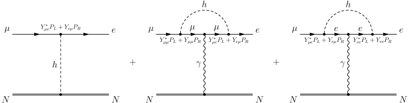
with the Lorentz indices and the electromagnetic field strength tensor. The Wilson coefficients and receive contributions from the two 1-loop diagrams shown in Fig. 1 (with the first one dominant), and a comparable contribution from Barr-Zee type 2-loop diagrams, see Fig. 12 in Appendix A. The complete one loop and two loop expressions are given in Appendix A.
In the approximation , only the first of the one-loop diagrams in Fig. 1 is relevant (in addition to the 2-loop diagrams). Using also and assuming , to be real, the expressions for the one-loop Wilson coefficients and simplify to (this agrees with [24])
| (13) |
The 2-loop contributions are numerically
| (14) |
where in the last step we used for the top Yukawa coupling , and we have normalized the results to for easier comparison. (By , we denote the top quark mass parameter in the renormalization scheme, GeV.) The analytical form of the Wilson coefficient can be found in Appendix A. The same result applies to with the replacement . The 2-loop contribution consists is dominated by two terms, the one with the top quark in the loop and of a somewhat larger contribution. They have opposite signs and thus part of contributions is cancelled. The end result has an increased sensitivity to the precise value of . For the 2-loop contribution is about four times as large as the 1-loop contribution, while for other values of (e.g., ) the 2-loop contribution can be an order of magnitude larger. Note that we keep complete 2-loop expressions [36], including the finite terms, while in [20, 24] only the leading log term of the top loop contribution was kept. Numerically, this amounts to an difference.
In terms of the Wilson coefficients and , the rate for is
| (15) |
Using a Higgs mass GeV and assuming , , we can then translate the experimental bound [37] into a constraint (see Table 1). The bound is relaxed if and/or are smaller than their SM values.
The expressions for and are obtained in an analogous way with the obvious replacements ( for the first and for the second in Eqs. (12), (13), (14), (15)). The experimental bound [37] then translates to and [37] to a constraint using the SM values for and . The bound is completely dominated by the two loop contribution, while for , the two loop and one loop contributions are comparable.
The decay can also be used to place a bound on the combination using the 1-loop Wilson coefficient (in agreement with [24])
| (16) |
As before, is obtained by replacing by . The 2-loop contribution is proportional to and . Setting them to zero, one obtains a bound .
III.2 Constraints from , ,

The decay can be generated through tree level Higgs exchange, see the diagram in Fig. 2 (left). However, the diagram is suppressed not only by the flavor violating Yukawa couplings and , but also by the flavor-conserving coupling . It is thus subleading compared to the higher order contributions: the 1-loop diagrams of the form shown in Fig. 1 and 2-loop diagrams like the ones shown in Fig. 12 (for ). These generate if the outgoing gauge boson is off-shell and “decays” to a muon pair. This general topology is shown in the right part of Fig. 2.
Integrating out the Higgs, the heavy gauge bosons and the top quark, these contributions match onto an effective Lagrangian. The full effective Lagrangian is similar to the one in Eq. (51) for conversion, but with quarks replaced by muons. Since a full evaluation of the 2-loop contributions is beyond the scope of this work, we will estimate the rate by including only the dimension 5 elecromagnetic dipole contributions of the form given in Eq. (12). For and , we use the same expressions as for , see Sec. III.1 and Appendix A. We evaluate these expressions at . We have checked that the neglected contributions are numerically smaller than the dipole terms at one loop. At two loops, to the best of our knowledge, a full evaluation of all potentially relevant diagrams is not available.
The corresponding expression for the flavor violating partial width of the is
| (17) |
where we have neglected terms additionally suppressed by the muon mass. The Wilson coefficients and are given approximately by Eqs. (13) and (14), with the 2-loop contribution dominating over the 1-loop one. In addition to (17) there are also contributions to the rate from effective flavor violating vertices induced at 1-loop by flavor violating Higgs exchanges. These have the same scaling in terms of masses and the Yukawas as (17), but are found to be numerically an order of magnitude smaller [38]. We therefore neglect them in the following.
The experimental bound [39] translates into a constraint for GeV and assuming that the diagonal Yukawa couplings , and have their Standard Model values. The decay thus leads to a weaker limit on , than , mainly because is suppressed by an additional power of compared to ).
Similarly, the constraints on , , , following from the processes and are weaker than the corresponding limits from and . The bounds in Table 1 are obtained using the experimental results [40] and [41]. We have also considered the process , but found that it yields a weaker limit than , mainly because of the smaller phase space.
III.3 Constraints from muonium–antimuonium oscillations
A bound state (called muonium ) can oscillate into an bound state (antimuonium ) through the diagram in Fig. 3. The time-integrated conversion probability is constrained by the MACS experiment at PSI [42] to be below , where the correction factor accounts for the splitting of muonium states in the magnetic field of the detector. It depends on the Lorentz structure of the conversion operator and varies between for operators and for operators [42]. Conservatively, we use the smallest value throughout. Since we will find that – oscillation constraints are much weaker than those from from and conversion, this approximation suffices for illustrative purposes.

The theoretical prediction for the conversion rate is governed by the mixing matrix element (see, e.g., [43])
| (18) |
where and are the spin orientations of particle . We can work in the non-relativistic limit here. For a contact interaction, the spatial wave function of muonium, , only needs to be evaluated at the origin. (Here is the electron–antimuon distance and is the muonium Bohr radius.) The resulting mass splitting between the two mass eigenstates of the mixed – system is [43],
| (19) |
and the time-integrated conversion probability is
| (20) |
The bound from the MACS experiment [42] then translates into .
III.4 Constraints from magnetic dipole moments

The CP conserving and CP violating parts of the diagram in Fig. 4 generate magnetic and electric dipole moments of the muon, respectively. Since the experimental value of the magnetic dipole moment, , is above the SM prediction at more than , also the preferred value for the flavor violating Higgs couplings will be nonzero.
The FV contribution to due to the -Higgs loop in Fig. 4 is (neglecting terms suppressed by or )
| (21) |
in agreement with [24]. The discrepancy between the measured value of and the one predicted by the Standard Model [39, 44],
| (22) |
could thus be explained if there are FV Higgs interactions of the size
| (23) |
(for the definition of the Yukawa couplings see Eq. (1)). This explanation of requires to be a factor of a few bigger than the SM value of the diagonal Yukawa, , and is in tension with limits from .333If the two loop contribution to is suppressed, e.g. due to a modification of the top Yukawa coupling, which could lead to significant cancellation between the 2-loop top and diagrams, there is a small region of parameter space in which flavor violating Higgs couplings could explain the discrepancy without being ruled out by the one loop constraint. We will, however, see below that even this case is disfavored by the LHC limit derived in this paper (see Sec. V.1). It is in further tension with the LHC limit extracted in Sec. V of this paper.
The measured could in principle also be explained by an enhanced flavor conserving coupling of the muon to the Higgs if . However, in this case decays would be enhanced to a level that is already ruled out by the searches at the LHC: From the search for the MSSM neutral Higgs boson one obtains a bound or [45].
III.5 Constraints from electric dipole moments
If the flavor violating Yukawa couplings in Fig. 4 are complex, the diagram shown there generates also an electric dipole moment (EDM) for the muon. The relevant term in the effective Lagrangian is
| (24) |
with the electric dipole moment given by (neglecting the terms suppressed by or )
| (25) |
in agreement with [24]. The experimental constraint [37] translates into the rather weak limit .
A similar diagram with electrons instead of muons on the external legs also contributes to the electron EDM, . The experimental constraint cm [37] translates into for a tau running in the loop, and into for a muon running in the loop.
III.6 Constraints from conversion in nuclei
Very stringent constraints on the FV Yukawa couplings and come from experimental searches for conversion in nuclei. The relevant tree-level and one-loop diagrams with one insertion of the FV Yukawa coupling are shown in Fig. 5. An effective scalar interaction arises already at tree level from the first diagram in Fig. 5, while vector and electromagnetic dipole contributions arise at one loop level. We give complete expressions for the tree level and one loop contributions in Appendix A.3. There are also two-loop contributions, similar to the ones discussed in Sec. III.1 in the context of . Numerically, the two-loop contributions are larger than the one loop ones because they are not suppressed by the small coupling but only by or the weak gauge coupling. They are in fact comparbale to the tree level contribution. Here, we always assume the diagonal Yukawa couplings to have their SM values. With this assumption, the tree level term is very sensitive to the strangeness content of the nucleon.
The bounds on the Yukawa couplings and from conversion in nuclei, including tree level, one-loop and two-loop contributions, are listed in Table 1.
One could potentially also obtain interesting limits on and from conversion in nuclei, even though this requires diagrams proportional to two FV Yukawa couplings, because the other constraints on these couplings are weak. The combinations , , and are constrained by conversion through 1-loop diagrams similar to the ones shown in Fig. 5, but with a running in the loop (see Eq. (54)). In the simplest case, , , with all Yukawa couplings real, the constraint is . This is almost, but not quite, competitive with the bound following from and decays, see Table 1.
III.7 LEP constraints
The Large Electron–Positron collider (LEP) is indirectly sensitive to the flavor violating Yukawa couplings and (with ) through the process , mediated by a -channel Higgs. The relevant observables here are the total cross sections and the forward–backward asymmetry of the final state leptons, both of which were measured as a function of the center-of-mass energy with uncertainties of order several per cent [46]. However, since the new physics contribution to is proportional to four powers of the off-diagonal Yukawa couplings, LEP limits cannot compete with constraints from flavor-violating decays like and and with the LHC constraints we derive in Section V. While a full derivation of LEP limits, including a careful treatment of the interference between Standard Model and non-standard contributions as well as a fit to the data points given in [46] is beyond the scope of this work, we have estimated that flavor-violating couplings are excluded by LEP.
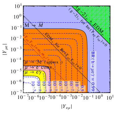
III.8 Allowed branching ratios for lepton flavor violating Higgs decays
In Fig. 6 we collect the above constraints on the values of , (upper left panel), , (upper right panel) and , (lower panel) and relate them to the predicted branching ratios for , and . The latter are given by
| (26) |
where , = , , , . The decay width , in turn, is
| (27) |
and the SM Higgs width is MeV for a 125 GeV Higgs boson [47]. In the panels of Fig. 6 we are assuming that at most one of non-standard decay mode of the Higgs is significant compared to the SM decay width.
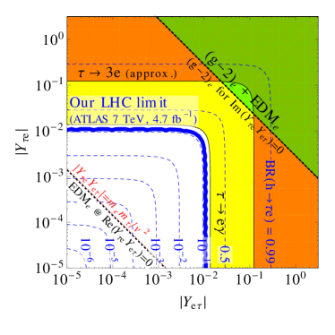
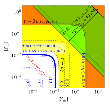
From Fig. 6 we see that given current bounds from and , branching fractions for or in the neighborhood of 10% are allowed. This is well within the reach of the LHC as we shall show in Sec. V. The allowed sizes of these two decay widths are comparable to the sizes of decay widths into nonstandard decay channels (such as the invisible decay width) that are allowed by global fits [48]. If there is no significant negative contribution to Higgs production through gluon fusion, one has , while allowing for arbitrarily large modifications of gluon and photon couplings to the Higgs leads to the constraint [48]. These two bounds apply without change also to , and .
In contrast to decays involving a lepton, the branching ratio for is extremely well constrained by , and conversion bounds, and is required to be below , well beyond the reach of the LHC.
IV Hadronic flavor violating decays of the Higgs
We next consider flavor violating decays of the Higgs to quarks. We first discuss two-body decays to light quarks, , , , , and then turn to FV three body decays mediated by an off-shell top, and as well as FV top decays to and . Our limits are summarized in Table 2.
| Technique | Coupling | Constraint |
|---|---|---|
| oscillations [49] | , | |
| oscillations [49] | , | |
| oscillations [49] | , | |
| oscillations [49] | , | |
| , | ||
| single-top production [50] | ||
| [51] | ||
| oscillations [49] | , | |
| , | ||
| neutron EDM [37, 52] | ||
IV.1 Flavor violating Higgs decays into light quarks

Flavor violating Higgs couplings to quarks can generate flavor changing neutral currents (FCNCs) at tree level, see Fig. 7 (a), and are thus well constrained by the measured , and mixing rates. Integrating out the Higgs generates an effective weak Hamiltonian, which for mixing is
| (28) |
Here we use the same notation for the Wilson coefficients as in [49] and display only nonzero contributions, which are
| (29) |
The results for , and mixing are obtained in the same way with the obvious quark flavor replacements. We can now translate the bounds on the above Wilson coefficients obtained in [49] into constraints on the combinations of flavor violating Higgs couplings as summarized in Table 2. We see that all Yukawa couplings involving only , , , , or quarks have to be tiny. The weakest constraints are those in the – sector, where flavor violating Yukawa couplings are still allowed. This would correspond to , which is still far too small to be observed at the LHC because of the large QCD backgrounds.
IV.2 Higgs decays through off-shell top and top decays to Higgs
Among the flavor violating Higgs couplings to quarks, the most promising place for new physics to hide are processes involving top quarks, such as the 3-body decay . Here, denotes either a charm quark or an up quark. The corresponding FV Yukawa couplings contribute at one loop to mixing through diagrams of the form of Fig. 7 (b). The corresponding Wilson coefficients in the effective Hamiltonian (28) are
| (30) | ||||||
| (31) | ||||||
| (32) |
where
| (33) |
and . Note that now also the operators (in the notation of [49]) have non-zero Wilson coefficients. By requiring that each individual operator is consistent with its mixing constraint, we derive the limits shown in the last part of Table 2. The constraints are much weaker than those on FV Higgs couplings involving only light quarks.
Strong constraints on and are also obtained from the non-observation of anomalous single top production. The flavor violating chromomagnetic operators
| (34) |
are generated trough loop diagrams similar to Fig. 1, but with leptons replaced by quarks and the photon replaced by a gluon. Here is the strong coupling constant, are the Gell-Mann matrices, is the gluon field strength tensor, and , are dimensionless effective coupling constants which depend on and according to
| (35) |
with the loop function given in Eq. (41). The analogous expression for is obtained by replacing and in . Note that in (35) we have assumed an EFT description with an on-shell gluon. Since this is only approximate, but we have checked that varying changes the bounds on , only by %. We have also made the approximation , which is obeyed even much better. Limits on , have been derived by the CDF and DØ collaborations [53, 50] and most recently by ATLAS [54]. In the notation of [54], we have . We obtain the constraints
| (36) |
We now translate these bounds into constraints on the decay width, which is given by (setting
| (37) |
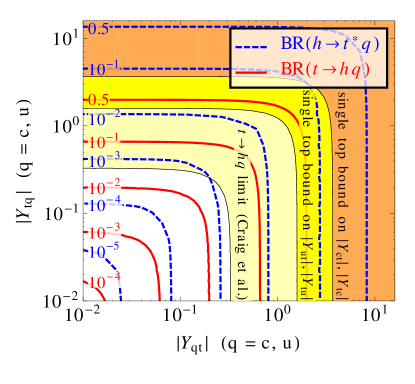
where is a CKM matrix element. The branching ratio for can be as large as , and the one for can be as shown in Fig. 8.
If the decay is non-negligible, so is the related non-standard top quark decay mode , the rate for which is given by (neglecting the charm mass)
| (38) |
Branching ratios for of several tens of per cent are perfectly viable and can be searched for, e.g. in the multi-lepton or channels. In fact, the strongest hint on Higgs couplings to are already coming from a CMS multi-lepton search which was recast in [51] to search for , giving a bound of 2.7% on the branching fraction of a top into a Higgs and a charm or up quark. This yields a limit of for or (see Fig. 8).
We have also calculated the branching ratios for the loop-induced processes , and (), which are in principle sensitive to and , but have found that even for , the current experimental bounds are satisfied [55].
In the above we have assumed that the weak phases of and are negligibly small. Otherwise an unacceptably large contribution to the neutron EDM is generated at 1-loop level with top and Higgs running in the loop. Eq. (25) with the replacements , and gives the -quark EDM , from which one can calculate the neutron EDM [56]. Using the 90% CL experimental bound [37] together with the estimate for the relation between the quark and neutron EDMs, Eq. (3.62) of [56], one obtains . To obtain this limit we have used the full one-loop expression for the quark EDMs rather than the approximation Eq. (25). For simplicity, we have neglected the contributions from chromomagnetic operators, which are similar in magnitude to the terms we keep. Including chromomagnetic terms and taking into account renormalization group running as well as using a conservative estimate of hadronic matrix elements, the authors of [52] obtain and .
We see that the limit on is much more stringent than the bounds on the absolute values of the same FV Yukawa couplings. In contrast, our estimates for the bounds from charm running in the loop, , and from -quark EDMs generated by the -quark and -quark running in the loop, and , respectively, are less stringent than the bounds from meson mixing, Table 2.
V Searching for flavor violating Higgs decays at the LHC
We next discuss possible search strategies for flavor violating Higgs decays at the LHC, focusing on the and decays. As shown in Fig. 6, these are among the least constrained of the couplings discussed in this paper, with a potential to modify the Higgs branching fractions significantly. They are sensitive to new particles with flavor violating couplings or to a secondary mechanisms of electroweak symmetry breaking such as additional Higgs doublets, and are thus good probes of new physics. Furthermore, they are also interesting final states as far as the potential for searches at the LHC is concerned.
The decay is quite similar to the standard model decay with one of the tau leptons decaying to a muon. This implies that existing SM Higgs searches, with only small or no modifications at all, can already be used to place bounds on the flavor violating decay. We thus first extract limits on and decays from an existing search in ATLAS. We then discuss how modifications to the search can lead to significantly improved sensitivity to flavor violating Higgs decays.
V.1 Extracting a bound on Higgs decays to and
We use the existing ATLAS search for in the fully leptonic channel [57] to place bounds on the and branching fractions. The reason we use fully leptonic events is that we can simulate the detector response to them more accurately than for events involving hadronic taus. It should, however, be noted that in the SM search in ATLAS, semi-hadronic events are about as sensitive as fully leptonic ones [57], and in CMS, the semi-hadronic mode provides even stronger limits [27]. The analysis in [57] uses the collinear approximation to reconstruct the invariant mass, i.e. it is assumed that the neutrino and the charged lepton emitted in tau decay are collinear. This approach is less optimized for than the maximum-likelihood method employed by CMS [58], but it is more model independent so that a substantial fraction of or decays would pass the cuts.444In fact, it may be interesting to apply the collinear approximation more often in resonance searches. A search for a collinear mass resonance can be sensitive to any particle which decays to boosted objects whose further decay may introduce missing energy. For simplicity we only use the ATLAS cuts optimized for Higgs production in vector boson fusion (VBF) since this channels provides the best sensitivity [57].
To derive limits we have generated 50,000 Monte Carlo events using MadGraph 5 v1.4.6 [59] for parton level event generation, Pythia 6.4 for parton showering and hadronization, and PGS [60] as a fast detector simulation. Combining the ATLAS lepton triggers and off-line cuts from [57], we select opposite sign dilepton events satisfying any of the following requirements: a muon pair with GeV for the leading muon and GeV for the subleading one, an electron pair with both GeV, or an electron and a muon with above 15 and 10 GeV, respectively. Electrons (muons) are accepted only if their pseudorapidity is . We require the invariant mass of the lepton pair to be GeV for pairs, or GeV for same flavor pairs. The missing is required to be above 20 (40) GeV for events ( or events). The azimuthal separation between the two leptons is required to be .
Additional cuts are placed with the goal of enriching the event sample in VBF events: at least two jets with above 40 GeV for the leading jet and above 25 GeV for the subleading jet are required, with the rapidity difference between the two leading jets above and the invariant mass GeV. We veto events with an additional jet with GeV and in the pseudorapidity region between the two leading jets.
The reconstructed invariant mass is calculated using the collinear approximation in which all invisible particles are assumed to be collinear with either of the two leptons. The fractions of the parent ’s momenta carried by the charged leptons are denoted by and . To be able to compare with ATLAS data from the search, we compute and assuming two neutrinos in the final state, even though yields only one. and are then obtained as the solutions of the transverse momentum equation , where are the transverse momenta of the charged leptons. Following [57], we require , which removes less than a per cent of events, but nearly 60% of our events. Thus, relaxing this cut would enhance the sensitivity to decays so long as it does not introduce large backgrounds. Nonetheless, we are still able to use the current search for to produce an interesting bound on .
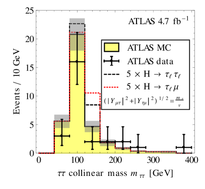
In Fig. 9 we show the background distribution for the collinear mass along with the expected shape of a LFV signals (scaled by a factor five for illustrative purposes only), and we compare to the observed data. The background expectation is taken from [57]. The backgrounds and the data in Fig. 9 include events for all three combinations of lepton flavor (even though our signal does not induce events) because only this information is available from ATLAS. For validation purposes, we have also simulated SM events, and comparing the rate and shape to Ref. [57] we find agreement to within 20%.
The signal is predominantly concentrated in the 120–160 GeV bin, so that the expected and observed limits on the flavor violating Yukawa couplings can be derived from a simple single-bin analysis. If we denote the number of expected background events by , the number of expected signal events for a given set of Yukawa couplings by , and the number of observed events by , the expected (observed) one-sided 95% C.L. frequentist limit on is defined by the requirement that the probability to observe () events is 5%. The relevant probability distribution of the data here is a Poisson distribution with mean . We can also include the systematic uncertainty in the 120–160 GeV bin, which is , in a conservative way by instead using a Poisson distribution with mean . Assuming the Higgs is produced with the Standard Model rates, this procedure leads to the bound on and the analogous bound on shown in Table 3 (see also Figure 6).
| 95% C.L. limit | ||||
|---|---|---|---|---|
| expected | 28% | 0.018 | 27% | 0.017 |
| observed | 13% | 0.011 | 13% | 0.011 |
V.2 Comparison of to
We now discuss the experimental differences and similarities between and decays to determine an optimized search strategy for the latter. We focus here on ,where denotes a that decays into a muon and two neutrinos and denotes a decaying hadronically. This channel is actively searched for, both at ATLAS [57] and at CMS [27], and is the most sensitive channel in the CMS search. (In ATLAS, fully leptonic events provide similar sensitivity to semi-hadronic ones.) It will also be the channel that we will devise a dedicated search for in the next subsection.
There are a few notable differences between the and decay channels:
-
•
Branching Ratios. The branching fraction for is , whereas for it is simply . For the signal for is thus a factor of larger.
-
•
Lepton Flavor. The flavor violating decays can lead to different rates for muons and electrons in the final state, whereas decays lead to equal and rates. Thus, if the various lepton flavor combinations were studied separately in the analyses, stronger bounds on flavor violating decays could be inferred.
-
•
Kinematics and Efficiencies. In decays the muon carries an average energy , while for it carries . Furthermore, in events the missing energy is roughly aligned with the hadronic . As a result the two channels can have different efficiencies given the same cuts. For example, in the VBF analysis described below (mimicking [27]) the efficiency for is a factor of lower than for events, mostly because many of the muons in the sample fall below the GeV cut.
-
•
Mass reconstruction. The LHC collaborations use highly optimized procedures for reconstructing the invariant mass. ATLAS uses the Missing Mass Calculator (MMC) from [58], while CMS uses an in-house maximum likelihood analysis [27]. These procedures use and the 3-momenta of the muon and the jet as input and estimate the neutrino momenta by assuming typical decay kinematics. For events, the MMC procedure returns an invariant mass with high efficiency () and gives a Higgs mass resolution of . If the event is not from but instead from , then i) the efficiency will be significantly lower since the kinematics can be completely inconsistent with a event, and ii) the reconstructed Higgs mass will be significantly higher as the MMC will assume that the hard muon is accompanied by two roughly collinear and hard neutrinos. This illustrates that a mass reconstruction procedure designed for the specific final state under consideration is mandatory to obtain the best possible sensitivity.
-
•
Backgrounds. The backgrounds for and events are similar, but because of the different invariant mass reconstruction techniques, the reconstructed background spectra will typically be harder for a analysis, which assumes three neutrinos in the final state, than for a analysis which assumes only one. This implies, for instance, that the peak from the background will appear at a invariant mass around 90 GeV in a search for , but well below (and thus further away from the signal peak) in a dedicated analysis.
These considerations show that the LHC is potentially more sensitive to flavor violating decays than to the SM channel. We now discuss a possible strategy for a tailored analysis.
V.3 A dedicated analysis
We now investigate the potential of a dedicated analysis which follows closely the CMS search for [27].555For semileptonically decaying , search strategies similar to the ones investigated in Ref. [61] for flavor violating decays could be used. The most important difference to that analysis will be a different algorithm for reconstructing the invariant mass. In particular, since the final state contains only one neutrino (from the hadronic ), this mass reconstruction can always be done exactly (i.e. the neutrino momentum can be determined) up to a two-fold ambiguity.
An important background for is , where either the decays into and one of the ’s decays further into a muon, or the decays into and one of the jets fakes a . Another important background is , followed by and a jet faking a . We neglect the small background, where a final state can come from a decay or be faked by a jet, and a muon can originate from a decay or from a leptonic decay. We also do not consider backgrounds from QCD multijet production because making reliable predictions for these events requires full detector simulations. Based on the CMS search [27] we expect them to be about as large as the background in the invariant mass region around 125 GeV.
To simulate the parton-level signal and background events, we use MadGraph 5 v1.4.6 [59], with an extended version of the Higgs Effective Theory model to include flavor-violating Higgs interactions. We use Pythia 6.4 for parton showering and hadronization and Delphes 2.0.2 [62] as a fast detector simulation. We have compared the detection efficiency as well as the fake rate from QCD jets in Delphes 2.0.2 to the corresponding performance indicators of several CMS tagging algorithm. With a tagging efficiency of and a fake rate between 0.2% at low and 1% at GeV, Delphes somewhat underestimates the performance of the CMS tagging algorithms [63]. (We have also studied tagging in PGS [60], but found it to be even farther away from what CMS can achieve.) To compensate for the imperfections in our treatment of -tagging, and for other inaccuracies in our simulations, we normalize our background distributions to the expected event numbers from [27], Table 2. We also normalize the signal using the same scaling factor as for the SM events.
In the analysis we require exactly one muon with GeV and in the final state and exactly one jet tagged as a hadronic decay with GeV and . The muon and the are required to have opposite charge. In [27], it was found that the best signal-to-background ratio is achieved in the events where the Higgs boson was produced through vector boson fusion (VBF), and we confirm this in our own simulations. To enrich the data sample in VBF events, we consider only events with a pair of jets , satisfying , , GeV and no other jets with GeV in the pseudorapidity region between the and . Here, is the pseudorapidity difference between the two jets and is the invariant mass of the jet pair. Non- jets are included in the analysis so long as their is above 30 GeV and their pseudorapidity is . In the CMS analysis [27], the transverse mass of the muon and the missing energy is restricted to be below 40 GeV in order to suppress the background. This works because in events, the muon and the neutrino from tend to be more back-to-back than in , where both ’s contribute to the missing energy. In , however, the muon and the missing energy also tend to be back-to-back, so that the cut also removes a large fraction of signal events.
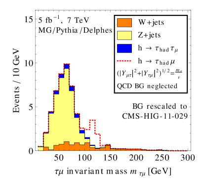
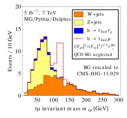
In light of this we show in Fig. 10 the expected signal and background rates for as a function of the – invariant mass both with and without the transverse mass cut. In computing for each event, we have used energy and momentum conservation to compute the -component of the neutrino momentum . There are two solutions to these equations, and we arbitrarily pick the smaller of the two. (We have checked that choosing the larger value for yields a very similar plot. This is related to the fact that , so that the ’s decay products are almost collinear.) As shown in the right panel of Fig. 10, dropping the transverse mass cut increases the plus jets background, but has the benefit of retaining more signal. The transverse mass distributions for signal and background is shown in Fig. 11. Assuming the plus jets and QCD backgrounds can be controlled reasonably, relaxing this cut may be worthwhile.
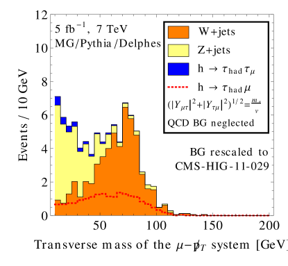
In summary, Fig. 10 shows that for flavor violating Yukawa couplings well allowed by low energy precision measurements, a spectacular signal can be expected in a dedicated search at the LHC. Such a search would cut deeply into the allowed parameter space of the flavor violation Higgs to couplings.
VI Conclusions
The LHC experiments have recently discovered a Higgs-like resonance with a mass around 125 GeV. In this paper we have examined the constraints on potential flavor violating couplings of this resonance, assuming it is indeed a scalar boson. In deriving the constraints we have assumed that that flavor changing neutral currents are dominated by the Higgs contributions, which may be thought of as a “simplified model” approach to flavor violation in light of the Higgs discovery. (In a complete model, cancellations between Higgs-induced flavor violation and flavor violation induced by other new physics is possible, but we do not pursue this possibility here.)
We have refined the indirect constraints on the flavor violating Yukawa couplings using results from rare decay searches, magnetic and electric dipole moment measurement, and the LHC. All constraints are summarized in Tables 1 and 2 and in Figs. 6 and 8. We have compared the bounds to the loose naturalness criterion that the off-diagonal Yukawa couplings are not much bigger then the geometric mean of diagonal terms, , and we have discussed to what extent the LHC can probe flavor violating decays of the form (or in the case of flavor violating top–Higgs couplings the decay ).
We draw the following conclusions:
Natural Flavor Violation.
The existing constraints involving only the first two generations of fermions, quarks or leptons, are strong enough that natural FV is already being probed by meson oscillations, conversion and . This conclusion also holds for FV couplings to quarks. In contrast, the FV couplings involving leptons or top quarks are allowed to have natural size (unless there is a large hierarchy between and ). This means that they are potentially observable, either at the LHC or in future low energy experiments.
Opportunities for the LHC.
The LHC has an opportunity to probe a large part of the allowed parameter space for and couplings. An LHC search in these channels would be very similar to the existing searches for , and recasting the latter already gives the best bounds on the flavor violating Yukawa couplings , , , and already now. A dedicated LHC search could improve the limits significantly. The reason why Higgs decays are very constraining is that the SM width of a 125 GeV Higgs boson is very small, MeV [47], so that the flavor violating couplings of the Higgs can have a significant effect. Another illustration of the LHC’s discovery potential for flavor violating Higgs couplings is that even the global fits of potential deviations in the dominant SM Higgs decay modes, , already give meaningful bounds on the FV Higgs decays. The results from these global fits are usually presented as bounds on the invisible decay width of the Higgs, but these bounds applies equally well to the sum of all the modes that have not been included in the fits. The constraint (at 95 % CL, with modest theory assumptions [48, 64, 65, 66]) is comparable to the constraints on and from precision searches of FCNCs in the lepton sector.
Acknowledgments
We thank Edward Boos, Alejandro Celis, Andreas Crivellin, Zackaria Chacko, Ricky Fok, Graham Kribs, Uli Haisch, Ethan Neil, Takemichi Okui, André Schöning and Ze’ev Surujon for valuable discussions, and LOT Polish Airlines for free internet access during a crucial phase of this project. This material is based upon work supported in part by the National Science Foundation under Grant No. PHYS-1066293 and the hospitality of the Aspen Center for Physics. JZ was supported in part by the U.S. National Science Foundation under CAREER Grant PHY1151392. Fermilab is operated by Fermi Research Alliance under contract DE-AC02-07CH11359 with the United States Department of Energy.
Appendix A Further details on leptonic FCNCs
In this appendix we collect detailed expressions for the FCNC processes and conversion in nuclei.
A.1 One loop expressions for , ,
The effective Lagrangian is given in Eq. (11). The Wilson coefficients are given by
| (39) | ||||
| (40) |
with the loop functions
| (41) | ||||
Here , and are the muon, tau and Higgs masses, respectively, is the 4-momentum of the photon, and is the Yukawa coupling matrix. Note that and differ only by the replacement . The first terms in Eqs. (39) and (40) arise from the first diagram in Fig. 1 (with a propagating in the loop), whereas the second terms arise from the second diagram (with a in the loop). Expanding in powers of and and keeping only the leading terms (so that only the first terms in (39), (40) contribute), the above expressions simplify to (13) if the diagonal Yukawa couplings are real. The simplified expressions for and (with a muon running in the loop) are obtained from (13) with trivial modifications, while the simplified expression for with a running in the loop is given in Eq. (16).
A.2 Two loop expressions for , and

At two loops there are numerically important diagrams with top or running in the loop, attached to the Higgs. Here we translate the results of [36] into our notation and adapt them to the case of . The diagrams with top and photon in the loops (see Fig. 12 top left) contributes as
| (42) |
while the -photon 2-loop contribution is
| (43) | ||||
Here we have already added the contributions from the would-be Goldstone bosons that get eaten by the . The contributions to are obtained from the above by replacing and .The loop functions are
| (44) | ||||
| (45) | ||||
| (46) |
the arguments are , , while the prefactor is
| (47) |
The contributions from the 2-loop diagrams with an internal are smaller as they are suppressed by . They are
| (48) | ||||
| (49) | ||||
with , , , , and the loop functions
| (50) |
The are obtained by replacing and in the above expressions. In addition there are also contributions called “set C” in [36]. An example for one of these diagrams is the last diagram in Fig. 12. Since the expressions for these diagrams are long we do not write them out explicitly. The “set C” contribution to is obtained from [36] by multiplying their Eq. (20) by and replacing .
The expressions are obtained by replacing and in the above expressions, while for the replacements are , and .
A.3 Details on conversion bounds
The most general effective Lagrangian for conversion in nuclei is [67]
| (51) | ||||
The Wilson coefficients and of the magnetic dipole operator are the same as the ones introduced for in Appendix A.2, with the replacements , . They receive contributions from one-loop and two-loop diagrams, with the two-loop diagrams being orders of magnitude larger numerically.
The vector operators are determined at one-loop by the last two diagrams in Fig. 5, with either a muon or an electron running in the loop. Explicitly, we find (with and )
| (53) |
Here, is the charge of quark , and , is given by Eq. (53) with the replacement . The loop function in (53) is
| (54) | ||||
where we have defined and . Note that we subtract the value of the one-loop vertex correction at , which gets absorbed into the wave function and mass renormalizations. and also receive two-loop contributions from diagrams similar to the ones relevant for , (see Fig. 12). To the best of our knowledge, analytic expressions for these contributions are not available in the literature, and are thus not included in our numerical results. While the one-loop vector contributions are smaller than the one-loop dipole ones in the conversion rate, and can be neglected, it would be desirable to also evaluate the two-loop vector terms in order to verify that all numerically important contributions have been taken into account.
All other Wilson coefficients in Eq. (51) are zero, .
When computing the conversion rate in nuclei care must be taken to account for the nuclear matrix elements , and and for the overlap of the initial muon wave function and the final state electron wave function. We follow [67] and obtain
| (55) | ||||
The electromagnetic penguin and vector contributions were already given above. Note that vector couplings to neutrons are absent due to the neutron’s vanishing electric charge. The scalar coefficients for proton and neutron coupling are given in terms of the quark level coefficients by
| (56) |
Here, the sum runs over all quark flavors, .
The nucleon matrix elements are calculated according to [68], but using an updated value for the nucleon sigma term MeV [69] (If the value of the nucleon sigma term is even smaller, as indicated by recent unquenched lattice results, our bounds would become weaker). The nucleon matrix elements are numerically
| (57) |
while the contributions from the heavier quarks are
| (58) |
with the same values for neutrons. In the above expressions, denotes a quark mass, is the proton mass, and is the neutron mass. The coefficients , , , and are overlap integrals of the muon, electron and nuclear wave function. They are tabulated for various target materials in [67]. The best limits are obtained from bounds on conversion on gold, ( CL) [70], for which in units of the overlap integrals are , , , , using the same distributions for neutrons and protons in the nucleus. For the SM capture rate, we use a value s-1 in the calculation [67].
References
- The ATLAS collaboration [2012a] The ATLAS collaboration (2012a), ATLAS-CONF-2012-093, available from http://cdsweb.cern.ch/record/1460439/files/ATLAS-CONF-2012-093.pdf.
- The CMS collaboration [2012] The CMS collaboration (2012), CMS-PAS-HIG-12-020, available from http://cdsweb.cern.ch/record/1460438/.
- Aad et al. [2012a] G. Aad et al. (The ATLAS Collaboration) (2012a), eprint 1207.7214.
- Chatrchyan et al. [2012a] S. Chatrchyan et al. (The CMS Collaboration) (2012a), eprint 1207.7235.
- Aaltonen et al. [2012] T. Aaltonen et al. (CDF Collaboration, D0 Collaboration) (2012), eprint 1207.6436.
- Bjorken and Weinberg [1977] J. Bjorken and S. Weinberg, Phys.Rev.Lett. 38, 622 (1977).
- McWilliams and Li [1981] B. McWilliams and L.-F. Li, Nucl.Phys. B179, 62 (1981).
- Shanker [1982] O. U. Shanker, Nucl.Phys. B206, 253 (1982).
- Barr and Zee [1990] S. M. Barr and A. Zee, Phys.Rev.Lett. 65, 21 (1990).
- Babu and Nandi [2000] K. Babu and S. Nandi, Phys.Rev. D62, 033002 (2000), eprint hep-ph/9907213.
- Diaz-Cruz and Toscano [2000] J. L. Diaz-Cruz and J. Toscano, Phys.Rev. D62, 116005 (2000), eprint hep-ph/9910233.
- Han and Marfatia [2001] T. Han and D. Marfatia, Phys.Rev.Lett. 86, 1442 (2001), eprint hep-ph/0008141.
- Blanke et al. [2009] M. Blanke, A. J. Buras, B. Duling, S. Gori, and A. Weiler, JHEP 0903, 001 (2009), eprint 0809.1073.
- Casagrande et al. [2008] S. Casagrande, F. Goertz, U. Haisch, M. Neubert, and T. Pfoh, JHEP 0810, 094 (2008), eprint 0807.4937.
- Giudice and Lebedev [2008] G. F. Giudice and O. Lebedev, Phys.Lett. B665, 79 (2008), eprint 0804.1753.
- Aguilar-Saavedra [2009] J. Aguilar-Saavedra, Nucl.Phys. B821, 215 (2009), eprint 0904.2387.
- Albrecht et al. [2009] M. E. Albrecht, M. Blanke, A. J. Buras, B. Duling, and K. Gemmler, JHEP 0909, 064 (2009), eprint 0903.2415.
- Buras et al. [2009] A. J. Buras, B. Duling, and S. Gori, JHEP 0909, 076 (2009), eprint 0905.2318.
- Agashe and Contino [2009] K. Agashe and R. Contino, Phys.Rev. D80, 075016 (2009), eprint 0906.1542.
- Goudelis et al. [2012] A. Goudelis, O. Lebedev, and J.-h. Park, Phys.Lett. B707, 369 (2012), eprint 1111.1715.
- Arhrib et al. [2012] A. Arhrib, Y. Cheng, and O. C. Kong (2012), eprint 1208.4669.
- McKeen et al. [2012] D. McKeen, M. Pospelov, and A. Ritz (2012), eprint 1208.4597.
- Azatov et al. [2009] A. Azatov, M. Toharia, and L. Zhu, Phys.Rev. D80, 035016 (2009), eprint 0906.1990.
- Blankenburg et al. [2012] G. Blankenburg, J. Ellis, and G. Isidori, Phys.Lett. B712, 386 (2012), eprint 1202.5704.
- Kanemura et al. [2006] S. Kanemura, T. Ota, and K. Tsumura, Phys.Rev. D73, 016006 (2006), eprint hep-ph/0505191.
- Davidson and Grenier [2010] S. Davidson and G. J. Grenier, Phys.Rev. D81, 095016 (2010), eprint 1001.0434.
- Chatrchyan et al. [2012b] S. Chatrchyan et al. (CMS Collaboration), Phys.Lett. B713, 68 (2012b), see also https://twiki.cern.ch/twiki/bin/view/CMSPublic/Hig11029TWiki, eprint 1202.4083.
- Ishimori et al. [2010] H. Ishimori, T. Kobayashi, H. Ohki, Y. Shimizu, H. Okada, et al., Prog.Theor.Phys.Suppl. 183, 1 (2010), eprint 1003.3552.
- Perez and Randall [2009] G. Perez and L. Randall, JHEP 0901, 077 (2009), eprint 0805.4652.
- Lees et al. [2012] J. Lees et al. (BaBar Collaboration) (2012), eprint 1205.5442.
- Fajfer et al. [2012] S. Fajfer, J. F. Kamenik, I. Nisandzic, and J. Zupan (2012), eprint 1206.1872.
- Buchmuller and Wyler [1986] W. Buchmuller and D. Wyler, Nucl.Phys. B268, 621 (1986).
- del Aguila et al. [2000a] F. del Aguila, M. Perez-Victoria, and J. Santiago, Phys.Lett. B492, 98 (2000a), eprint hep-ph/0007160.
- del Aguila et al. [2000b] F. del Aguila, M. Perez-Victoria, and J. Santiago, JHEP 0009, 011 (2000b), eprint hep-ph/0007316.
- Cheng and Sher [1987] T. Cheng and M. Sher, Phys.Rev. D35, 3484 (1987).
- Chang et al. [1993] D. Chang, W. Hou, and W.-Y. Keung, Phys.Rev. D48, 217 (1993), eprint hep-ph/9302267.
- Beringer et al. [2010] J. Beringer et al. (Particle Data Group), Phys. Rev. D86, 010001 (2010).
- Goto et al. [2015] T. Goto, R. Kitano, and S. Mori (2015), eprint 1507.03234.
- Nakamura et al. [2010] K. Nakamura et al. (Particle Data Group), J. Phys. G37, 075021 (2010).
- Bellgardt et al. [1988] U. Bellgardt et al. (SINDRUM Collaboration), Nucl.Phys. B299, 1 (1988).
- Hayasaka et al. [2010] K. Hayasaka, K. Inami, Y. Miyazaki, K. Arinstein, V. Aulchenko, et al., Phys.Lett. B687, 139 (2010), eprint 1001.3221.
- Willmann et al. [1999] L. Willmann, P. Schmidt, H. Wirtz, R. Abela, V. Baranov, et al., Phys.Rev.Lett. 82, 49 (1999), eprint hep-ex/9807011.
- Clark and Love [2004] T. Clark and S. Love, Mod.Phys.Lett. A19, 297 (2004), eprint hep-ph/0307264.
- Bennett et al. [2006] G. Bennett et al. (Muon G-2 Collaboration), Phys.Rev. D73, 072003 (2006), eprint hep-ex/0602035.
- The ATLAS collaboration [2012b] The ATLAS collaboration (2012b), ATLAS-CONF-2012-094, available from cdsweb.cern.ch/record/1460440/files/ATLAS-CONF-2012-094.pdf.
- Alcaraz et al. [2006] J. Alcaraz et al. (ALEPH Collaboration, DELPHI Collaboration, L3 Collaboration, OPAL Collaboration, LEP Electroweak Working Group) (2006), eprint hep-ex/0612034.
- Dittmaier et al. [2012] S. Dittmaier, S. Dittmaier, C. Mariotti, G. Passarino, R. Tanaka, et al. (2012), eprint 1201.3084.
- Carmi et al. [2012] D. Carmi, A. Falkowski, E. Kuflik, T. Volansky, and J. Zupan (2012), eprint 1207.1718.
- Bona et al. [2008] M. Bona et al. (UTfit Collaboration), JHEP 0803, 049 (2008), eprint 0707.0636.
- Abazov et al. [2010] V. M. Abazov et al. (D0 Collaboration), Phys.Lett. B693, 81 (2010), eprint 1006.3575.
- Craig et al. [2012] N. Craig, J. A. Evans, R. Gray, M. Park, S. Somalwar, et al. (2012), eprint 1207.6794.
- Gorbahn and Haisch [2014] M. Gorbahn and U. Haisch (2014), eprint 1404.4873.
- Aaltonen et al. [2009] T. Aaltonen et al. (CDF Collaboration), Phys.Rev.Lett. 102, 151801 (2009), eprint 0812.3400.
- Aad et al. [2012b] G. Aad et al. (ATLAS Collaboration), Phys.Lett. B712, 351 (2012b), eprint 1203.0529.
- Chatrchyan et al. [2012c] S. Chatrchyan et al. (CMS Collaboration) (2012c), eprint 1208.0957.
- Pospelov and Ritz [2005] M. Pospelov and A. Ritz, Annals Phys. 318, 119 (2005), eprint hep-ph/0504231.
- Aad et al. [2012c] G. Aad et al. (ATLAS Collaboration) (2012c), eprint 1206.5971.
- Elagin et al. [2011] A. Elagin, P. Murat, A. Pranko, and A. Safonov, Nucl.Instrum.Meth. A654, 481 (2011), eprint 1012.4686.
- Alwall et al. [2011] J. Alwall, M. Herquet, F. Maltoni, O. Mattelaer, and T. Stelzer, JHEP 1106, 128 (2011), eprint 1106.0522.
- Conway et al. [2009] J. Conway et al., PGS—Pretty Good Simulation (2009), http://physics.ucdavis.edu/ conway/research/software/pgs/pgs4-general.htm.
- Davidson et al. [2012] S. Davidson, S. Lacroix, and P. Verdier (2012), eprint 1207.4894.
- Ovyn et al. [2009] S. Ovyn, X. Rouby, and V. Lemaitre (2009), eprint 0903.2225.
- The CMS collaboration [2011] The CMS collaboration (2011), cMS-PAS-TAU-11-001, available from http://cdsweb.cern.ch/record/1337004/.
- Espinosa et al. [2012] J. R. Espinosa, M. Muhlleitner, C. Grojean, and M. Trott (2012), eprint 1205.6790.
- Djouadi et al. [2012] A. Djouadi, A. Falkowski, Y. Mambrini, and J. Quevillon (2012), eprint 1205.3169.
- Giardino et al. [2012] P. P. Giardino, K. Kannike, M. Raidal, and A. Strumia (2012), eprint 1207.1347.
- Kitano et al. [2002] R. Kitano, M. Koike, and Y. Okada, Phys.Rev. D66, 096002 (2002), eprint hep-ph/0203110.
- Ellis et al. [2008] J. R. Ellis, K. A. Olive, and C. Savage, Phys.Rev. D77, 065026 (2008), eprint 0801.3656.
- Young and Thomas [2010] R. D. Young and A. W. Thomas, Nucl. Phys. A844, 266c (2010), eprint 0911.1757.
- Bertl et al. [2006] W. H. Bertl et al. (SINDRUM II Collaboration), Eur.Phys.J. C47, 337 (2006).