Anisotropic Flow and Viscous Hydrodynamics

Abstract

We report part of our recent work on viscous hydrodynamics with consistent phase space distribution $f(x,{\bf p})$ for freeze out. We develop the gradient expansion formalism based on kinetic theory, and with the constraints from the comparison between hydrodynamics and kinetic theory, viscous corrections to $f(x,{\bf p})$ can be consistently determined order by order. Then with the obtained $f(x,{\bf p})$, second order viscous hydrodynamical calculations are carried out for elliptic flow $v_{2}$.

1 Introduction

Relativistic hydrodynamics is an important theoretical tool in heavy ion collisions. Especially it successfully reproduces the observed elliptic flow $v_{2}$. In the past several years, with respect to the updated understanding of collective phenomena in heavy-ion collisions, two major progresses have been made in hydrodynamical models. One is the realization of fluctuations in initial state[1], which leads to the practically used event-by-event hydrodynamics[2, 3]. And correspondingly many new types of anisotropic flow, such as dipole flow $v_{1}$[4] and triangular flow $v_{3}$[1, 5], are studied. The other one is the inclusion of viscous corrections[6].

In practice, although ideal hydrodynamics has been found effective in characterizing the collective medium expansion, viscous corrections are not negligible[7]. One particular example of viscous corrections to hydrodynamics is the viscous damping of elliptic flow[8, 9, 10].

Many attempts have been made in the investigation of the viscous corrections to hydrodynamics[8, 9, 10]. Since first order viscous hydrodynamics suffers from the causality problem(see for example[11]), most of the established viscous hydrodynamical models have contained second order viscous terms in the equations of motion, such as Israel-Stewart theory. Recently, in an important paper, Baier and his collaborators(BRSSS) developed second order viscous hydrodynamical theory with conformal symmetry assumption[12]. Hydrodynamical simulation to the medium expansion in heavy ion collisions is achieved by solving hydrodynamical equations of motion, with respect to the specified initial conditions. Observables are obtained then by freeze out process. Due to the correspondence between hydrodynamics and kinetic theory, freeze out process also needs viscous corrections, and the corrections have to be constrained so that they are consistent with hydrodynamics itself. In particular, in Cooper-Fryer formula, this is reflected in the determination of the phase-space distribution function $f(x,{\bf p})$. However, to the knowledge of authors, this constraints have not been systematically discussed in the literature through second order, and this will be the main subject of this paper. For more details, refer to [13].

The paper is organized as follows. The theoretical formalism is constructed by reviewing viscous effects in kinetic theory and hydrodynamics in section 2. In section 3 the determination of phase-space distribution function is discussed. Hydrodynamical simulations with consistent form of $f(x,{\bf p})$ is carried out, and elliptic flow $v_{2}$ is calculated at RHIC energy, in section 4. Our conclusions are summarized in section 5.

2 Kinetic Theory and Hydrodynamics

A liquid system out of equilibrium can be approached through either transport theory or hydrodynamics, provided that the non-equilibrium part can be seen as perturbations. As a result, in order to sustain the continuity around freeze out, there must be a determined correspondence between kinetic theory and hydrodynamics. This correspondence originates the constraints on distribution function $f(x,{\bf p})$. In terms of the dependence on transverse momentum $p_{T}$, one can generally fix $\delta f$ by the moment method[14], in which $\delta f$ is decomposed into moment expansion and cut at a certain order. The widely accepted form, for example,

$$\delta f_{\pi}=\frac{n_{p}(1\pm n_{p})}{2(e+\mathcal{P})T^{2}}p^{\mu}p^{\nu}\pi_{\mu\nu},$$ (1)

is obtained by a fourteen-momentum method. However there are two flaws in this form for realistic simulations. First, in actual simulations $\pi_{\mu\nu}$ is taken from second order hydrodynamical calculations, while $\delta f_{\pi}$ is computed using a first order approximation. Second, and more importantly, the $p_{T}$ dependence in $\delta f$ has been investigated in [15], and found to vary based on microscopic dynamics. Although the quadratic ansatz (i.e. Eq. (1)) is appropriate for collisional energy loss, it fails in the case where radiative energy loss dominates.

In kinetic theory, the viscous corrections $\delta f(x,{\bf p})$ corresponds to the viscous corrections to hydrodynamics, i.e., stress tensor $\pi^{\mu\nu}$, so it also depends on gradient expansion. In this way, following Chapman-Enskog method[14] where expansion in gradients is used to find asymptotic form of the solution to Boltzmann equation, $\delta f(x,{\bf p})$ can be determined order by order. When relaxation time approximation can be taken into account, form of $\delta f$ is analytically solvable for the specified viscous hydrodynamics. In this paper, we take relaxation time approximation and determine $\delta f(x,{\bf p})$ through second order in gradients, with respect to BRSSS hydrodynamics.

The matrix convention we use throughout the paper is $(-,+,+,+)$. $p^{\mu}$ is used for four-momentum. And for the sake of convenience, we introduce a tilde on a quantity from time to time to indicate it as dimensionless. In the derivation of hydrodynamics, tensor index is always split into temporal and spatial parts. Since flow four-velocity $u^{\mu}=\gamma(1,\vec{v})$ is purely temporal in the local rest frame(LRF), the decomposition is then realized based on $u^{\mu}$ and the projection operator $\Delta^{\mu\nu}=u^{\nu}u^{\nu}+g^{\mu\nu}$. For derivative operator we have $\partial^{\mu}=u^{\mu}D+\nabla^{\mu}$, with $D=u^{\mu}\partial_{\mu}$ and $\nabla^{\mu}=\Delta^{\mu\nu}\partial_{\nu}$ representing pure time and space derivatives in LRF respectively. A further decomposition according to rotation group is also considered comparing to the existed tensor form in hydrodynamics, so the indices of a tensor in brackets $\left\langle\ldots\right\rangle$ stand for being symmetric, (projection operator) traceless and transverse,

$$A^{\mu\ldots\left\langle\ldots\alpha\ldots\beta\ldots\right\rangle\ldots\nu}=A^{\mu\ldots\left\langle\ldots\beta\ldots\alpha\ldots\right\rangle\ldots\nu}$$ (2)

$$A^{\mu\ldots\left\langle\ldots\alpha\ldots\beta\ldots\right\rangle\ldots\nu}\Delta_{\alpha\beta}=0$$ (3)

$$A^{\mu\ldots\left\langle\ldots\alpha\ldots\right\rangle\ldots\nu}\Delta_{\alpha\beta}=0$$ (4)

More details of the decomposition can be found in [13].

2.1 Hydrodynamics

In Chapman-Enskog expansion, the so-called solubility condition[14] relates spatial gradients and temporal derivatives. This is actually equivalent to hydrodynamical equations of motion $\partial_{\mu}T^{\mu\nu}=0$. In the current section we will derive the viscous corrections through second order to BRSSS hydrodynamical equations of motion.

The energy-momentum tensor of viscous hydrodynamics reads

$$T^{\mu\nu}=eu^{\mu}u^{\nu}+\mathcal{P}\Delta^{\mu\nu}+\pi^{\mu\nu}{\,,}$$ (5)

where $\pi^{\mu\nu}$ is the viscous correction to stress tensor. In this paper, the bulk viscosity $\zeta=0$ and baryon chemical potential $\mu_{B}=0$. Up to second order viscous corrections, BRSSS[16] determined that the possible forms of the gradient expansion in the stress tensor in a conformal liquid are

$$\pi^{\mu\nu}=-\eta\sigma^{\mu\nu}+\eta\tau_{\pi}\left[\left\langle D\sigma^{\mu\nu}\right\rangle+\frac{1}{d-1}\sigma^{\mu\nu}\nabla\cdot u\right]+\lambda_{1}\left\langle\sigma^{\mu}_{\phantom{\mu}\lambda}\sigma^{\nu\lambda}\right\rangle+\lambda_{2}\left\langle\sigma^{\mu}_{\phantom{\mu}\lambda}\Omega^{\nu\lambda}\right\rangle+\lambda_{3}\left\langle\Omega^{\mu}_{\phantom{\mu}\lambda}\Omega^{\nu\lambda}\right\rangle{\,,}$$ (6)

where $\sigma^{\mu\nu}=2\langle\nabla^{\mu}u^{\nu}\rangle$ and the vorticity tensor is defined as

$$\Omega^{\mu\nu}=\frac{1}{2}\Delta^{\mu\alpha}\Delta^{\nu\beta}\left(\nabla_{\alpha}u_{\beta}-\nabla_{\beta}u_{\alpha}\right){\,.}$$ (7)

$(\tau_{\pi},\lambda_{1},\lambda_{2},\lambda_{3})$ are corresponding second order transport coefficients. $d=4$ is the number of space-time dimensions. Then equations of motion according to Eq. (6) can be formulated as

$$De= -(e+\mathcal{P})\nabla\cdot u+\frac{\eta}{4}\sigma_{\mu\nu}\sigma^{\mu\nu}+O(\nabla^{3}){\,,}$$ (8)

$$Du_{\mu}= -\frac{\nabla_{\alpha}\mathcal{P}}{e+\mathcal{P}}+\frac{u_{\mu}D\sigma^{\mu\nu}\Delta_{\alpha\nu}}{e+\mathcal{P}}-\frac{\Delta_{\alpha\nu}\nabla_{\mu}\sigma^{\mu\nu}}{e+\mathcal{P}}+O(\nabla^{3}){\,.}$$ (9)

Note that the temporal derivatives of the flow velocity $u^{\mu}$ and the energy density $e$ are written in terms of spatial gradients through second order, while higher order terms are neglected.

2.2 Kinetics

To determine the viscous corrections to the distribution function, the strategy is to solve the kinetic equations in a relaxation time approximation order by order in the gradient expansion:

$$f(x,{\bf p})\equiv n_{\bf p}(x,{\bf p})+\delta f(x,{\bf p})=n_{\bf p}(x)+\delta f_{(1)}+\delta f_{(2)}+O(\nabla^{3}){\,,}$$ (10)

where $n_{\bf p}(x)$ is equilibrium distribution, which depends on the space-time coordinates through the dimensionless combination $p\cdot u/T=\tilde{p}\cdot u$. In classical limit, $n_{\bf p}(x)=\mbox{exp}[p\cdot u(x)/T(x)].$ In a relaxation time approximation the Boltzmann equation reads

$$p^{\mu}\partial_{\mu}f_{\bf p}(x)=-\frac{T^{2}}{\tilde{C}_{\bf p}}\left[f-n(p\cdot u_{*}(x)/T_{*}(x))\right]{\,,}$$ (11)

where the dimensionless coefficient $\tilde{C}_{\bf p}$ is related to the canonical momentum dependent relaxation time $\tau_{R}$,

$$\tilde{C}_{{\bf p}}=-T^{2}\,\frac{\tau_{R}(-p\cdot u)}{p\cdot u}{\,.}$$ (12)

Following the convention used in [15], the canonical relaxation time is proportional to $(-\tilde{p}\cdot u)^{1-\alpha}$, where $\alpha$ lies generally between the quadratic ansatz limit($\alpha=0$) and linear ansatz limit ($\alpha=1$). We have

$$\tilde{C}_{{\bf p}}=c_{0}(-\tilde{p}\cdot u)^{-\alpha},$$ (13)

with $c_{0}$ to be fixed by shear viscosity (see below). The parameters $u^{*\mu}(x)$ and $T^{*}(x)$ which appear in the Eq. (11) are equal at leading order to the temperature and flow velocities ($T$ and $u^{\mu}$). They satisfy the Landau matching conditions, i.e. ,

$$\left(\nu\int\frac{d^{3}p}{(2\pi)^{3}E_{\bf p}}p^{\mu}p^{\nu}\delta f(u^{*},T^{*})\right)u^{*}_{\mu}=0,\qquad\left(\nu\int\frac{d^{3}p}{(2\pi)^{3}E_{\bf p}}p^{\mu}p^{\nu}n_{\bf p}(u^{*},T^{*})\right)u^{*}_{\mu}=eu^{*\nu}.$$ (14)

So there exist the expansion

$$T^{*}(X)\equiv T(X)+\delta T^{*}{\,,}$$ (15)

$$u^{*\mu}(X)\equiv u^{\mu}(X)+\delta u^{*\mu}{\,,}$$ (16)

with $\delta T^{*}=\sum_{n=1}\delta T_{(n)}$ and $\delta u^{*\mu}=\sum_{n=1}\delta u^{\mu}_{(n)}$ indicating corrections from all higher order gradients. Expanding $n_{p}^{*}$ (with an obvious notation) we find correspondingly,

$$n_{\bf p}^{*}\equiv n_{\bf p}+\delta n_{p}^{*}\quad\mbox{and}\quad\delta n_{{\bf p}}^{*}=n_{\bf p}^{\prime}\left[\frac{p\cdot\delta u_{*}}{T}-E_{\bf p}\frac{\delta T_{*}}{T^{2}}\right],$$ (17)

where here and in the following a prime stands for the derivative on $\tilde{p}\cdot u$. $\delta n_{\bf p}^{*}$ with higher order gradients is important for the determination of viscous correction $\delta f$, as will be shown in the next section. Eq. (14), together with the correspondence between kinetic theory and hydrodynamics,

$$\nu\int\frac{d^{3}p}{(2\pi)^{3}E_{\bf p}}p^{\mu}p^{\nu}\delta f(u^{*},T^{*})=\pi^{\mu\nu}{\,,}$$ (18)

constrains the solution of Boltzmann equation $f(x,{\bf p})$.

3 Determination of $\delta f$

We substitute the expansion Eq. (10) into the kinetic equation Eq. (11) and equate orders. In doing so we use the hydrodynamic equations of motion to write time derivatives of $T(x)$ and $u(x)$ in terms of spatial gradients of these fields, see Eq. (8). Indeed, with the help of these equations of motion, up to first order in gradient,

$$p^{\mu}\partial_{\mu}n_{\bf p}=+n_{\bf p}^{\prime}\frac{p^{\mu}p^{\nu}}{2T}\sigma_{\mu\nu}+O(\nabla^{2}){\,.}$$ (19)

The terms linearly proportional to the $\sigma_{\mu\nu}$ is ultimately responsible for shear viscosity.

Collecting all the terms of first order in gradient for $\delta f$ we obtain the preliminary first order solution

$$\delta f_{(1)}= -\tilde{C}_{\bf p}\;n_{\bf p}^{\prime}\;\frac{p^{\mu}p^{\nu}\sigma_{\mu\nu}}{2T^{3}}+\delta n_{{\bf p}(1)}^{*}.$$ (20)

But Eq. (20) is not completed until the constant coefficient $c_{0}$, the form of $\delta u^{\mu}_{(1)}$ and $\delta T_{(1)}$ are determined through constraint conditions Eq. (14) and Eq. (18). Obviously there exist the trivial solution $\delta u^{\mu}_{(1)}=0$ and $\delta T_{(1)}=0$ to Eq. (14), and then from Eq. (18) we find,

$$\eta=\frac{T^{3}}{15}B_{1}.$$ (21)

$B_{1}$ is a dimensionless constant from the integral,

$$B_{1}(\alpha)=\nu\int\frac{d^{3}\tilde{p}}{(2\pi)^{3}\tilde{E}_{\bf p}}(\tilde{p}\cdot u)^{4}[n_{\bf p}^{\prime}\tilde{C}_{\bf p}].$$ (22)

It only depends on the underlying microscopic dynamics in terms of $\alpha$. We will encounter three more similar constants,

$$B_{2}(\alpha) =\nu\int\frac{d^{3}\tilde{p}}{(2\pi)^{3}\tilde{E}_{\bf p}}(\tilde{p}\cdot u)^{6}[n_{\bf p}^{\prime}\tilde{C}_{\bf p}]^{\prime}\tilde{C}_{p}{\,,}$$ (23)

$$B_{3}(\alpha) =-\nu\int\frac{d^{3}\tilde{p}}{(2\pi)^{3}\tilde{E}_{\bf p}}(\tilde{p}\cdot u)^{5}[n_{\bf p}^{\prime}\tilde{C}_{\bf p}]\tilde{C}_{p}{\,,}$$ (24)

$$B_{4} =-\nu\int\frac{d^{3}\tilde{p}}{(2\pi)^{3}\tilde{E}_{\bf p}}(\tilde{p}\cdot u)^{3}[n_{\bf p}^{\prime}]{\,.}$$ (25)

$c_{0}$ is then the solution to Eq. (21), and it is interesting to know that for a massless gas and in the quadratic ansatz limit, $c_{0}=\eta/s$.

We extend the derivation to second order $\delta f_{(2)}$, then

$$\delta f_{(2)}= -\tilde{C}_{\bf p}\;n_{\bf p}^{\prime}\;\frac{\eta}{s}\;\frac{1}{T^{4}}\Big{[}p\cdot u\,p_{\mu}\left(2\left\langle\sigma^{\mu\nu}\nabla_{\nu}lnT\right\rangle+\left\langle\Delta^{\mu}_{\alpha}\nabla_{\beta}\sigma^{\alpha\beta}\right\rangle\right)+\frac{(p\cdot u)^{2}}{4(d-1)}\sigma^{2}\Big{]}$$

$$-\frac{\tilde{C}_{\bf p}}{T^{2}}\;p^{\mu}\partial_{\mu}\delta f_{(1)}+\delta n_{{\bf p}(2)}^{*}{\,.}$$ (26)

Clearly there are three sources of contributions, those generated from $\delta f_{(1)}$ in Boltzmann equation, from second order corrections to flow velocity and temperature and from second order hydrodynamics equations of motion. The dominant term is from $p^{\mu}\partial_{\mu}\delta f_{(1)}$, since in Boltzmann equation the derivative gives rise to one higher order dependence on $p_{T}$ simultaneously. To write $\delta f_{(2)}$ explicitly we decompose the resulting tensors into irreducible tensors of the rotation group in the LRF ; [13] provides a few more details. Straightforward then from (3), with somewhat tedious algebra, we obtain,

$$\delta f_{(2)}=\; \frac{[n^{\prime}\tilde{C}_{\bf p}]^{\prime}\tilde{C}_{\bf p}}{4T^{2}}\tilde{p}^{\mu}\tilde{p}^{\nu}\tilde{p}^{\alpha}\tilde{p}^{\beta}\left\langle\sigma_{\mu\nu}\sigma_{\alpha\beta}\right\rangle-\frac{[n^{\prime}\tilde{C}_{\bf p}]\tilde{C}_{\bf p}}{2T^{2}}\tilde{p}^{\mu}\tilde{p}^{\nu}\tilde{p}^{\alpha}\left[3\left\langle\sigma_{\mu\nu}\nabla_{\alpha}lnT\right\rangle+\left\langle\nabla_{\alpha}\sigma_{\mu\nu}\right\rangle\right]$$

$$+\tilde{p}^{\mu}\tilde{p}^{\nu}\left\langle\sigma_{\mu}^{\lambda}\sigma_{\nu\lambda}\right\rangle\left[\frac{[n^{\prime}\tilde{C}_{\bf p}]^{\prime}\tilde{C}_{\bf p}}{7T^{2}}(\tilde{p}\cdot u)^{2}+\frac{[n^{\prime}\tilde{C}_{\bf p}]\tilde{C}_{\bf p}}{2T^{2}}\tilde{p}\cdot u\right]$$

$$+\tilde{p}^{\nu}\tilde{p}^{\nu}\left\langle\sigma_{\mu\lambda}\Omega^{\lambda}_{\nu}\right\rangle\frac{[n^{\prime}\tilde{C}_{\bf p}]\tilde{C}_{\bf p}}{T^{2}}\tilde{p}\cdot u-\tilde{p}^{\mu}\tilde{p}^{\nu}\left[\left\langle D\sigma_{\mu\nu}\right\rangle+\frac{\sigma_{\mu\nu}}{3}\nabla\cdot u\right]\frac{[n^{\prime}\tilde{C}_{\bf p}]\tilde{C}_{\bf p}}{2T^{2}}\tilde{p}\cdot u$$

$$+\tilde{p}_{\mu}\tilde{p}\cdot u\left[\frac{\eta}{s}\frac{n^{\prime}\tilde{C}_{\bf p}}{T^{2}}+\frac{[n^{\prime}\tilde{C}_{\bf p}]\tilde{C}_{\bf p}}{5T^{2}}\tilde{p}\cdot u\right]\left[2\left\langle\sigma^{\mu\nu}\nabla_{\nu}lnT\right\rangle+\left\langle\Delta^{\mu}_{\alpha}\nabla_{\beta}\sigma^{\alpha\beta}\right\rangle\right]$$

$$+\sigma^{2}\left[-\frac{\eta}{s}\frac{n^{\prime}\tilde{C}_{\bf p}}{T^{2}}\frac{(\tilde{p}\cdot u)^{2}}{12}+\frac{[n^{\prime}\tilde{C}_{\bf p}]^{\prime}\tilde{C}_{\bf p}}{4T^{2}}\frac{2(\tilde{p}\cdot u)^{4}}{15}+\frac{[n^{\prime}\tilde{C}_{\bf p}]\tilde{C}_{\bf p}}{2T^{2}}\frac{(\tilde{p}\cdot u)^{3}}{3}\right]$$

$$+\delta n_{{\bf p}(2)}^{*}{\,.}$$ (27)

The first line in (3) does not contribute to $\pi^{\mu\nu}$, since all tensor structure from momentum integral are orthogonal to these terms in brackets. Besides the already fixed parameter $c_{0}$, we still need to determine second order corrections to flow velocity and temperature, by solving Landau-Lifshitz matching condition. And we find that these following solutions satisfy all the constraint conditions, up to second order in gradient,

$$\delta u^{\mu}_{(2)} =-\frac{3}{B_{4}T^{2}}\left[-\frac{\eta}{3s}B_{1}+\frac{B_{3}}{12}\right]\left[2\left\langle\sigma^{\mu\nu}\nabla_{\nu}lnT\right\rangle+\left\langle\Delta^{\mu}_{\alpha}\nabla_{\beta}\sigma^{\alpha\beta}\right\rangle\right]$$ (28)

$$\delta T_{(2)} =-\frac{\sigma^{2}}{B_{4}T}\left[-\frac{\eta}{s}\frac{B_{1}}{12}+\frac{B_{2}}{30}-\frac{B_{3}}{6}\right]{\,.}$$ (29)

As a by-product of the constraint condition Eq. (18), we also recognize that

$$\eta\tau_{\pi}=\frac{T^{2}B_{3}}{15},\quad\lambda_{1}=\eta\tau_{\pi}\left[\frac{2B_{2}}{7B_{3}}+1\right],\quad\lambda_{2}=-2\eta\tau_{\pi},\quad\lambda_{3}=0.$$ (30)

These relations are in the consistent range with those discussed in [17]. In particular, all these non-trivial second order transport coefficients are non-free parameters in our formalism, as long as $\eta/s$ is fixed. This reduces the number of free parameters in hydrodynamical calculations, and thus quite significant for the recent study on the extraction of $\eta/s$[18].

4 Viscous Hydrodynamic Simulation and Elliptic Flow

The simulation of hydrodynamics in code needs solving hydrodynamical equations of motion. For viscous hydrodynamics, for the convenience of computation, the algorithm is introduced by approximation. In BRSSS formalism, up to second order in gradients, Eq. (6) can be rewritten as

$$\pi^{\mu\nu}=-\eta\sigma^{\mu\nu}-\tau_{\pi}\left[\langle D\pi^{\mu\nu}\rangle+\frac{4}{3}\pi^{\mu\nu}\nabla\cdot u\right]-\frac{\lambda_{1}}{\eta}\langle\pi_{\lambda}^{\;\mu}\sigma^{\lambda\nu}\rangle-\frac{\lambda_{2}}{\eta}\langle\pi_{\lambda}^{\;\mu}\Omega^{\lambda\nu}\rangle+O(\nabla^{3}),$$ (31)

such that a linearized equation for $\pi^{\mu\nu}$, which is approximately correct if all higher order gradients are neglected, is obtained. Then together with general hydrodynamical equations of motion, $\partial_{\mu}T^{\mu\nu}$=0, and appropriately selected equation of state, we have a complete set of equations for the unknown variables, $(\pi^{\mu\nu},e,u^{\mu})$. There are two options for the equation of state in our calculations. For theoretical interest we can consider conformal equation of state(CEOS). Although CEOS does not have the accurate description for real medium expansion in heavy ion collisions, it has the conformal symmetry as assumed in BRSSS hydrodynamics. The previously used lattice equation of state(LEOS) by Romatschke and Luzum[9] is also tested. The details of the algorithm can be found in [13]. For the initial state, smooth initial condition is considered. As indicated by several groups[3, 19], event fluctuations in the calculations of $v_{2}$ can be safely ignored. A constant temperature freeze out scheme is taken, with $T_{fo}=150$ MeV.

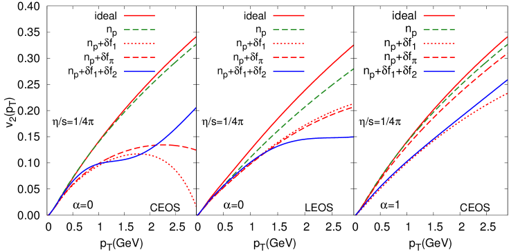
Figure 1: Differential $v_{2}$ results from various viscous hydrodynamical calculations, $b=6.8$ fm.

The effects of including consistent $\delta f$ in freeze out procedure can be best seen in the results of elliptic flow. In Fig. 1 the results of a series of calculations are shown. Compare to ideal hydrodynamics, viscous hydrodynamics indeed damps the generated $v_{2}$, and a major fraction of the damping is from $\delta f$. This is reflected in the difference between the calculated $v_{2}$ with equilibrium distribution function $n_{p}$ and that with $n_{p}+\delta f$’s. The complete and consistent calculation with respect to BRSSS hydrodynamics needs also $\delta f_{(2)}$ correction. However, in the quadratic ansatz limit and conformal equation of state the corresponding $v_{2}$(left panel in Fig. 1) quickly becomes unreliable when $p_{T}$ goes up to $1.5$ GeV. This is due to the dramatic increase of viscous corrections at large $p_{T}$ region, and has already been discussed in the first order case with $\delta f_{\pi}$[10]. But now that $\delta f_{(2)}$ has higher $p_{T}$($p_{T}^{4}$) dependence, this effect is much stronger. In another way, we can estimate the magnitude of viscous corrections by calculating the spectrum. Then gradient expansion formalism fails when $\delta f$ contributes to spectrum no longer perturbatively. As seen in the left panel in Fig. 2, we find similarly for CEOS and quadratic ansatz limit, $p_{T}>1.5$GeV region is beyond the feasibility of our formalism.

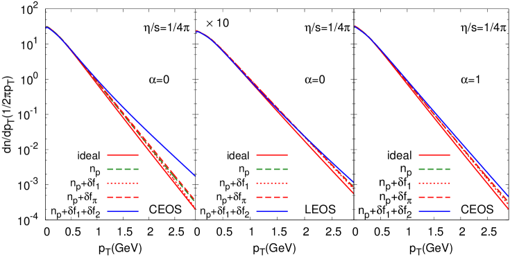
Figure 2: Spectrum from various viscous hydrodynamical calculations, $b=6.8$ fm. Note that a factor of 10 has been multiplied in the case of LEOS to make it on the same scale.

Changing equation of state or the $\alpha$ dependence, however, can help solving the problem to some extent. As seen in the two other panels in Fig. 1 and Fig. 2, viscous corrections are smaller. On one hand these changes extend our reliable calculation to higher $p_{T}$ region. On the other hand, realistic medium in heavy ion collisions has equation of state more close to LEOS, and also quadratic ansatz limit does not necessarily reflect the real microscopic dynamics. So as expected, second order corrections in $\delta f$ lead to extra corrections to calculated observables.

5 Discussions and Future Work

We have presented a formalism for the derivation of viscous corrections to phase space distribution function at freeze out. With respect to BRSSS hydrodynamics, from this formalism we have obtained the consistent form of $\delta f_{(2)}$, and checked its impact on hydrodynamical simulations. $\delta f_{(2)}$ affects the results as corrections, and the corrections increase with $p_{T}$. But for LEOS or $\alpha=1$, the corresponding corrections are as small as perturbations. This is expected from the gradient expansion of the formalism we are following. At last, this dependence on $\alpha$ verifies the claim in [15] that quadratic ansatz may be questionable in real calculations.

One important property of higher order viscous corrections in $f(x,{\bf p})$, is its higher $p_{T}$ dependence. This plays a crucial role in the study of anisotropic flow for two aspects. 1. This makes the flow results more sensitive to $\eta/s$. 2. This makes higher order anisotropic flow $v_{n}$ more sensitive. Both of these aspects have positive effects on the extraction of $\eta/s$ from heavy ion collisions. And this will be the main subject of our future work.

References

References

- [1] Alver B and Roland G 2010 Phys.Rev. C81 054905 (Preprint 1003.0194)
- [2] Schenke B, Jeon S and Gale C 2011 Phys.Rev.Lett. 106 042301 (Preprint 1009.3244)
- [3] Qiu Z and Heinz U W 2011 Phys.Rev. C84 024911 (Preprint 1104.0650)
- [4] Teaney D and Yan L 2011 Phys.Rev. C83 064904 (Preprint 1010.1876)
- [5] Alver B H, Gombeaud C, Luzum M and Ollitrault J Y 2010 Phys.Rev. C82 034913 (Preprint 1007.5469)
- [6] Teaney D 2003 Phys.Rev. C68 034913 (Preprint nucl-th/0301099)
- [7] Danielewicz P and Gyulassy M 1985 Phys.Rev. D31 53–62
- [8] Dusling K and Teaney D 2008 Phys.Rev. C77 034905 (Preprint 0710.5932)
- [9] Luzum M and Romatschke P 2008 Phys.Rev. C78 034915 (Preprint 0804.4015)
- [10] Song H and Heinz U W 2008 Phys.Rev. C77 064901 (Preprint 0712.3715)
- [11] Romatschke P 2010 Int.J.Mod.Phys. E19 1–53 (Preprint 0902.3663)
- [12] Baier R, Romatschke P, Son D T, Starinets A O and Stephanov M A 2008 JHEP 0804 100 (Preprint 0712.2451)
- [13] Teaney D and Yan L , In progress
- [14] De Groot S, Van Leeuwen WA e and Van Weert C 1980
- [15] Dusling K, Moore G D and Teaney D 2010 Phys.Rev. C81 034907 (Preprint 0909.0754)
- [16] Policastro G, Son D and Starinets A 2001 Phys.Rev.Lett. 87 081601 (Preprint hep-th/0104066)
- [17] York M A and Moore G D 2009 Phys.Rev. D79 054011 (Preprint 0811.0729)
- [18] Shen C, Bass S A, Hirano T, Huovinen P, Qiu Z et al. 2011 J.Phys.G G38 124045 (Preprint 1106.6350)
- [19] Gardim F G, Grassi F, Luzum M and Ollitrault J Y 2012 Phys.Rev. C85 024908 (Preprint 1111.6538)