Radiative energy loss and spectra for viscous hydrodynamics
Abstract
This work investigates the first correction to the equilibrium phase space distribution and its effects on spectra and elliptic flow in heavy ion collisions. We show that the departure from equilibrium on the freezeout surface is the largest part of the viscous corrections to . However, the momentum dependence of the departure from equilibrium is not known a priori, and it is probably not proportional to as has been assumed in hydrodynamic simulations. At high momentum in weakly coupled plasmas it is determined by the rate of radiative energy loss and is proportional to . The weaker dependence leads to straighter curves at the same value of viscosity. Further, the departure from equilibrium is generally species dependent. A species dependent equilibration rate, with baryons equilibrating faster than mesons, can explain “constituent quark scaling” without invoking coalescence models.
I Introduction
When two ultra-relativistic nuclei collide, they leave behind a region of high energy-density QCD matter, whose properties we would like to understand better. The initial geometry of the QCD matter is set by the overlap region of the two colliding nuclei. Generally, the nuclei collide at finite impact parameter rather than head-on. In this case the initial geometry is not a disk, but is an “almond shaped” ellipse. (The short and long axis of the initial almond are taken as the and axes respectively.) The production mechanism of the QCD matter is local and knows nothing of this global geometry. Therefore, to a first approximation the initial stress tensor will be locally azimuthally symmetric. Subsequently, if there are no reinteractions the produced matter will free stream to the detector; the initial geometry will have no influence on the evolution, and the angular distribution of the final observed hadrons will also be azimuthally symmetric. On the other hand, if there are strong interactions which maintain local thermal equilibrium, the pressure gradients in the direction will be larger than in the direction, an anisotropy in the collective flow will develop, and ultimately an anisotropy in the momentum spectrum of the final hadrons will be observed.
The final momentum anisotropy is characterized experimentally by , the second harmonic of the azimuthal distribution of the produced particles with respect to the reaction plane. Experimentalists have measured as a function of transverse momentum , particle type, and impact parameter Adams:2005dq ; Adcox:2004mh ; Back:2004je ; Arsene:2004fa . These results are surprisingly well described by ideal hydrodynamics idealhydro , which amounts to the approximation that the interactions are fast enough to maintain the matter in equilibrium from an early time until hadronic freeze-out. There are some limits to this success. First, the measured falls below the ideal hydrodynamic prediction for momenta larger than . Second, the hydro fit fails to reproduce certain relative trends observed in the baryon and meson elliptic flows. These trends are compactly summarized by “constituent quark scaling” Abelev:2008ed ; Adare:2006ti ; coalesence which generally has been attributed to a kind of coalescence of constituent quarks Lin:2001zk ; Molnar:2003ff ; Greco:2003xt ; Fries:2003vb . Here we will argue that the first corrections to equilibrium can clarify both of these shortcomings without the need for a coalescence model.
To quantify the corrections to ideal hydrodynamics it is important to study nonideal (viscous) hydrodynamics. In the last two years there has been a major push in this direction Baier:2006gy ; Romatschke:2007jx ; Romatschke:2007mq ; Song:2007fn ; Dusling:2007gi ; Huovinen:2008te ; Song:2007ux ; Bozek:2007qt . These studies have used various formalisms and have studied variations of with respect to the input shear viscosity, the model for the initial geometry, and various other nuisance parameters. However, we want to point out here that these studies have all made a common assumption about the way that the asymmetry in the stress tensor is manifested in the particle distribution after freezeout. In particular, the particle distribution after freezeout is locally of the form where is the equilibrium distribution and is the first correction. All groups have assumed that and that the coefficient of proportionality is independent of particle type.
In this paper we will argue that this assumption matters, and that it is far from secure. After an overview of the issue in the next section, in Section III we will discuss the physics which establishes the momentum dependence of and its behavior in several theories. We will see that while the most studied theories give , the most QCD-like theories do not. Then we explore the behavior of multi-component plasmas in Section IV. We see there that the viscous corrections for different species are generically different. This fact can account for the “constituent quark scaling” observed in the baryon and meson elliptic flows without any reference to the hadronization process. We then make our concluding remarks. Some technical material is postponed to appendices.
Throughout, we will denote 4-vectors with capital letters and use for their 3-vector components, for their energy components, and for . Our metric convention is [–,+,+,+], so that . We use tilde to indicate momenta scaled by temperature, . We will mostly write for the equilibrium distribution function, but will occasionally use when common convention dictates its use. The appropriate statistics will be clear from context.
II Overview
The energy momentum tensor is given by the sum of its ideal and dissipative parts111We use Landau-Lifshitz conventions to fix in terms of four components of . The other six independent components of can always be accommodated by a satisfying .
| (1) |
and obeys the equation of motion,
| (2) |
In the first-order (or Navier-Stokes) approximation the dissipative part of the stress energy tensor in the local rest frame is
| (3) |
where is the shear viscosity, and we use to indicate that the bracketed tensor should be symmetrized and made traceless. It is well known that the first order theory is plagued with difficulties such as causality violations and instabilities Hiscock:1983zz ; Hiscock:1985zz . In order to circumvent these issues a second order theory is required. The most commonly used second order relativistic viscous hydrodynamics is due to Israel and Stewart IS . For technical reasons we use a theory developed by Öttinger and Grmela OG ; Ottinger . The two theories are qualitatively the same (i.e. for sufficiently small relaxation times they both approach the first order theory). To streamline the presentation we postpone the details of our hydrodynamic model to Appendix A and refer to previous work Dusling:2007gi .
The solutions to the hydrodynamic equations yield the underlying temperature and flow profiles in the presence of viscosity. Particle spectra are then computed using the Cooper-Frye CF formula
| (4) |
where and is the freeze-out hypersurface taken as a surface of constant energy density in this work. For a system out of equilibrium is not the equilibrium distribution function but also contains viscous corrections,
| (5) |
where is the ideal Bose/Fermi distribution function. The form of is constrained by the requirement that be continuous across the freeze-out hypersurface:
| (6) |
Dropping from the final particle spectra is inconsistent as it leads to a discontinuity in . The form for which satisfies continuity in the local rest frame is proportional to and is traditionally parametrized by 222In actual simulations is treated as a dynamical variable in a second order fluid formalism. Then to first order one can make the replacement, . There has been no attempt to systematically include through second order in hydrodynamic simulations.
| (7) | |||||
| (8) |
where we have distinguished and by the argument of the function. One moment of is fixed by the shear viscosity (see below) but otherwise is an arbitrary function of . To date all works on viscous hydrodynamics have taken the quadratic Ansatz and have usually worked in a Boltzmann approximation
| (9) |
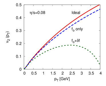
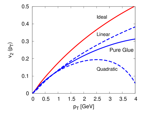
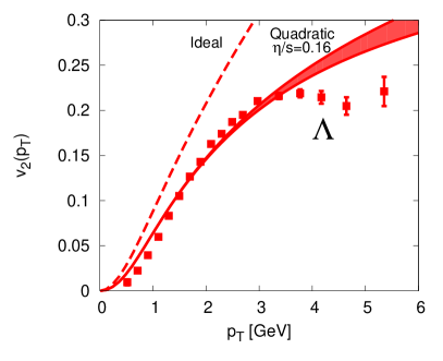
Let us look at typical results for as shown in Fig. 1. The curve labeled ‘Ideal’ shows the result using ideal hydrodynamics (i.e. . The curve labeled ‘’ shows the resulting elliptic flow from the viscous evolution (the solution of Eqs. (2),(3) and (69)) but without including the viscous correction to the distribution function. In other words, this shows how the viscous correction to the temperature and flow profiles manifests itself in the particle spectra. Only modest corrections to the spectra are found. As already emphasized, this result is unphysical since dropping violates continuity of the stress tensor. Last, the curve labeled ‘’ also takes into account, using the quadratic Ansatz. The viscous correction to the distribution function dominates the reduction in at large . That means that the term is responsible for a significant part of the effects of viscosity in the particle spectra.
This being the case, it is imperative to perform a systematic study on the form of the viscous correction as well as its effect on elliptic flow. Most of this paper will discuss the form of the viscous correction appearing in weakly-coupled QCD. Although this is not a theory of hadronizing QCD, it is one theory where quantitative first-principle calculations can be performed. One of our major findings is that not all models of energy loss give the same predictions for the off-equilibrium distribution function.
III Form of in several theories
In this section we consider a number of theories, to show that while the dependence is expected in some cases, other functional dependence is expected in others, including weakly coupled QCD and a hadron (resonance) gas. The theories where we can make a definite statement about the functional form of are all described by kinetic theory. Since freeze-out is defined as the point where scatterings go from being common to being rare on the time scale of the evolution of the system, we generally expect that, just before freezeout, kinetic theory should be a reasonable description.
Within kinetic theory, the distribution function is determined by a Boltzmann equation,
| (10) |
where is the collision operator. In equilibrium the distribution function obeys
| (11) |
To determine the first viscous correction , we work in a vicinity of the local rest frame , and substitute into Eq. (10) keeping terms first order in the spatial derivatives
| (12) |
Here denotes the linearized collision operator, the collision operator expanded to first order in . In writing Eq. (12) we have used ideal hydrodynamics and thermodynamic relations to rewrite time derivatives as spatial derivatives, and we have neglected gradients proportional which are responsible for the bulk viscosity Teaney:2009qa . Eq. (12) is an integral equation for which can be solved by various methods.
Since the first viscous correction is a scalar and must be proportional to the the strains, the most general form for the viscous correction in the local rest frame can be parametrized by the function as in Eq. (7). Close to equilibrium the first viscous correction determines the strains
| (13) |
which ultimately yields a relation between between the shear viscosity and the viscous correction
| (14) |
This is the only general constraint on the functional form of the viscous distribution function. To proceed further we must specify completely the form of the linearized collision operator, which we will do in the context of various model theories.
III.1 Simplest model: relaxation time approximation
The simplest model (really a cartoon) for the collision operator is the relaxation time approximation,
| (15) |
where is the momentum dependent relaxation time to be specified. Substituting this form for the collision operator into Eq. (12), and working in a Boltzmann approximation yields the following form for :
| (16) |
Note however that the relaxation time is in general energy dependent. In different theories, might show different functional dependence on . Without details about the dynamics of the theory in question, we can only parametrize the viscous correction. Here we will discuss a massless classical gas where and parameterize the relaxation time (or the distribution function) with a simple power law
| (17) |
The constant, , is determined through Eq. (14):
| (18) |
There are two limiting cases for the functional form of the the relaxation time approximation, and . The momentum dependence of the relaxation time in these extreme cases is
| (21) |
Most theories will lie between these two extreme limits.333There are exceptions to this rule. For instance, in a gas of Goldstone bosons far below the symmetry breaking scale one expects , since the cross section grows rapidly with energy, . Loosely speaking, if the energy loss of high momentum particles grows linearly with momentum, one expects a relaxation time independent of momentum, . On the other hand if the energy loss approaches a constant , the relaxation time will grow with the particle momentum .
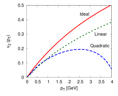
Fig. 2 shows the elliptic flow computed using these two functional forms for the first viscous correction. It is important to emphasize that shear viscosity is the same in both cases. Examining these figures, we see that the integrated elliptic flow is largely insensitive to the functional form of the first viscous correction. This is because the integrated is primarily determined by the hydrodynamic variables , which are independent of the functional dependence of the relaxation time Teaney:2009qa . The differential elliptic flow is sensitive to the rate of equilibration especially above .
III.2 Scalar theory
Scalar field theory has been described at length by Jeon Jeon:1994if , who rigorously derived the Boltzmann equation and its collision kernel and then solved for numerically. But if we make the approximation of Boltzmann statistics, we can actually solve for in closed form.
First the non-linear Boltzmann equation with Bose-Einstein statistics is
| (22) |
where the transition rate (including a final state symmetry factor) is
| (23) |
and we have used the traditional short hand, . After linearizing, the linearized collision integral is
| (24) |
At this point we will make the Boltzmann assumption by neglecting the stimulation factors, , and using, . Then we will try a solution of the form
| (25) |
assuming that or . Substituting this form into the integral equation (Eq. (12) and Eq. (24)), and performing the integrals yields (see Appendix B)
| (26) |
Thus, taking , the quadratic form in Eq. (25) has provided an exact solution solution to the linearized integral equation. The viscosity is in a Boltzmann approximation.
Physically, this happens because of the form of the scattering cross-section. Since and , the cross-section scales as the inverse of the particle’s energy. The typical scattering is nearly randomizing, but high energy particles undergo fewer scatterings than low-energy ones. Therefore we find the same functional form as for momentum diffusion but for very different reasons.
This example from scalar field theory, together with the example of momentum diffusion (see Section III.3.1 below), are the reason that most people assume the quadratic ansatz, should hold.
III.3 Weakly coupled pure-glue QCD
In this section we will use the Boltzmann equation for pure-glue QCD in three approximation schemes to calculate the first viscous correction. First we will consider a leading approximation where the dynamics can be summarized by a Fokker-Planck equation which describes the momentum diffusion of quasi-particles. In this limit we will find that the viscous correction is quadratic at large momentum, . Next we will consider the QCD Boltzmann equation but consider only collisions and neglect collinear radiation. In this limit, we will find that the viscous correction at large momentum behaves as . Finally, we will also include collinear radiation in the Boltzmann equation as is necessary in a complete leading order treatment Arnold:2001ba ; Arnold:2002zm . We will find that collinear radiation controls the relaxation of the high momentum modes and asymptotically we have , where the coefficient of proportionality is set by the rate of transverse momentum broadening, . The impatient reader may skip to Section III.3.4 which summarizes the results of these three approximation schemes.
III.3.1 Momentum diffusion in a leading log treatment
In a leading log approximation, is considered a large number and the dynamics describes soft Coulomb scattering. Each soft collision involves a small momentum transfer of order , but these collisions happen relatively frequently at a rate of (neglecting logarithms). Thus a typical particle with momentum will diffuse in momentum space and equilibrate on a time scale of . The resulting Boltzmann equation linearized around equilibrium can be written as a Fokker-Planck equation Arnold:2000dr ; Juhee
| (27) |
where is the drag coefficient of a high momentum gluon in this approximation scheme Thoma:1992kq ; Braaten:1991jj
| (28) |
The precise form of the gain terms has been given in Arnold:2000dr ; Juhee , but only involves the spherical harmonic components of , and . In the hydrodynamic limit considered here is proportional to a traceless rank 2 tensor () and these gain terms vanish. Substituting the form of Eq. (7) into Eq. (27) leads to the following equation for :
| (29) |
We are not aware of a closed form solution to this equation, but we can find a solution for at large momentum. Making the approximation , we find that
| (30) |
solves this equation. This is the well known quadratic Ansatz.
III.3.2 Boltzmann equation with collisions
We next will consider the QCD Boltzmann equation but we will neglect collinear radiation. We emphasize that this is not a consistent approximation scheme. Nevertheless, it illustrates clearly the relative roles of hard collisions and inelastic processes in determining the functional form of in the relevant sub-asymptotic regime.
The linearized Boltzmann equation is the same as Eq. (24), but the squared matrix element is
| (31) |
which describes gluon scattering after summing over all spins and colors and dividing by the gluon degeneracy factor . These matrix elements must be dynamically screened using Hard Thermal Loops. A procedure which is consistent at leading order (where the Debye mass is small) but which makes a reasonable estimate when the Debye mass is not small has also been described in Arnold:2003zc , and we can follow exactly the numerical procedure of that reference to find .444Some minor technical difficulties are discussed in the next section. We can also study the asymptotic behavior more directly. At asymptotically large momentum where may be considered large, Appendix B shows that
| (32) |
The constant in front of the log is related to , the rate of collisional energy loss of a gluon with momentum ,
| (33) |
In a leading approximation the loss rate is Bjorken:1982tu ; Braaten:1991jj
| (34) |
as is rederived in Appendix B. The above asymptotic form agrees well with the numerical solution of the Boltzmann equation.
III.3.3 A leading order treatment at asymptotically large momenta
Early calculations of the shear viscosity in pure-glue QCD found , that is, Baym:1990uj ; Heiselberg:1994vy . However this is because they were leading-log treatments, which reduced to momentum diffusion discussed above. It was realized in Arnold:2001ba ; Arnold:2002zm that inelastic number changing processes are only suppressed by a log, but are enhanced at large energy by a factor of and dominate equilibration for .
This should not be a surprise. After all, if we think about “equilibration” (energy loss) in QED, we find that although the leading order mechanism for the energy loss of a high energy electron is ionization (elastic scattering), bremsstrahlung actually dominates the loss rate. This is the case because in bremsstrahlung the energy lost per scattering can scale with the incident energy, rather than being incident energy independent as is the case with ionization. As a result, the penetration depth of an electromagnetic shower scales only logarithmically with the incident energy, i.e. the relaxation time is constant up to logs, . If the same behavior occurred in QCD we would expect the linear Ansatz to hold, .
The current understanding of energy loss in perturbative QCD is that the high energy behavior lies between these extremes. High-energy particles in a QCD plasma lose energy predominantly by inelastic gluon radiation and the time scale for energy loss is short compared to the time scale for momentum diffusion (“jet broadening”). In particular it was shown by Baier et al that for the rate of (inelastic) energy loss scales with the incident energy as , with the half-integer power arising from the LPM suppression Baier:1996kr ; Baier:1996sk . This implies a “relaxation time” which scales as , and therefore Arnold:2003zc . Let us see how this emerges in the behavior of pure-glue QCD.
The point is that the Boltzmann equation for a gluon plasma possesses both an elastic scattering term and an inelastic effective scattering term,
| (35) |
This equation was first solved at leading order in by Arnold, Moore and Yaffe to determine the shear viscosity Arnold:2003zc . Their approach involved writing a multi-parameter Ansatz for in terms of a basis of test functions. While the determination of improves quadratically with the test function basis, the determination of improves only linearly. Therefore to get good accuracy out to requires the use of a large basis of functions. We find a basis of eight functions is sufficient and the behavior is already clear with such a basis.555In fact we find greatly improved convergence of the large-momentum behavior, both in terms of basis set size and numerical integration precision, by changing the test functions of Arnold:2003zc to a set which show the correct large momentum asymptotic behavior by multiplying defined in Eq.(2.32) of the reference by .
We can also directly establish the asymptotic form of the solution. At asymptotically high momentum near collinear bremsstrahlung dominates the equilibration of gluons. We therefore look at the Boltzmann equation including only splittings,
| (36) |
The relevant collision integral for near collinear joining and splitting of gluons at leading order in was worked out in Arnold:2002ja :
| (37) |
and is given in terms of the splitting function for . In general this splitting function involves the solution of an integral equation which includes the LPM effect. However, in the deep LPM regime Arnold:2008zu where can be treated as small, the following leading log result for the splitting function can be obtained,
| (38) |
The above splitting function contains the transport parameter , which characterizes the typical transverse momentum squared transferred to the particle per unit length. With the above splitting function we show in Appendix C that the solution of the off-equilibrium distribution function at asymptotically large momentum is
| (39) |
III.3.4 Summary of weakly coupled pure glue QCD
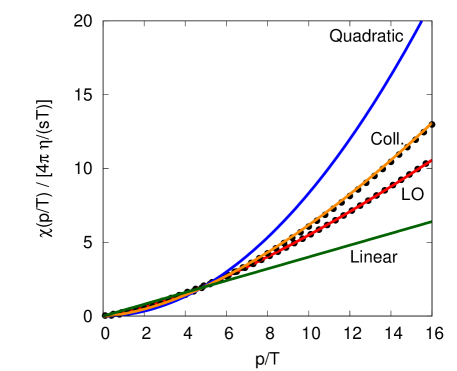
Let us now summarize some of the main features of the off-equilibrium dynamics of pure glue QCD at weak coupling. In the previous three sections we looked at the behavior of the off-equilibrium correction for pure glue QCD in various approximation schemes, deriving asymptotic behavior in each case. These asymptotics are listed in Table 1. In this section we wish to focus on the phenomenologically more interesting region where the equilibrating parton has intermediate energies (). In this case one must resort to numerical solutions of the Boltzmann equation which we present in Fig. 3.
To summarize Fig. 3, we will discuss the curves from top to bottom starting with the “Quadratic” curve. In the leading approximation the linearized Boltzmann equation simplifies to a differential equation, Eq. (29). The numerical solution to this has been worked out in Heiselberg:1994vy ; Arnold:2000dr ; Juhee and is well described for all momenta by the asymptotic quadratic form, . The numerical result will be presented in a forthcoming work Juhee , and for now we show the quadratic result as the solid blue line (color online). Next we considered QCD with the gluon scattering matrix element at leading order. The agreement between the asymptotics derived in the previous section and the numerical solution can be found in Appendix B. At intermediate momentum we show the numerical solution of the Boltzmann equation without inelastic processes as the data points under the curve labeled “Coll.”. The solid curve is the result of a power law fit at intermediate momentum, . In the leading order (LO) treatment when bremsstrahlung is included, we find further equilibration of the gluons and our numerical results are reasonably described by the fit, . Finally, the linear ansatz is also shown in Fig. 3 for comparison.
One can now ask how the observed of pure glue at leading order will affect the viscous corrections to elliptic flow. First of all, as we have already shown, the integrated will change marginally. The differential , on the other hand, will be largely affected at higher . This result is shown in Fig. 4 along with the quadratic and linear Ansätze for comparison.
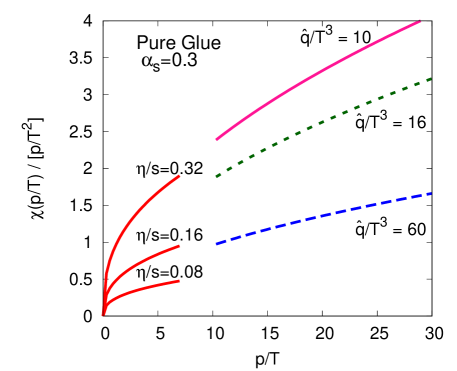
The above considerations have shown that the relaxation of the high energy tail of the distribution is largely controlled by energy loss. The low / intermediate momentum region is constrained by the shear viscosity via Eq. (14). The strength of the off equilibrium correction is controlled by two non-perturbative parameters: at low momentum and at high momentum. This is clearly seen by looking at the forms of we have found for pure glue QCD at leading order,
| (42) |
In Fig. 5 we show plots of for various choices of the non-perturbative parameters and . The main point to take away is the need for a consistency between and such that the low and high momentum regions of can merge smoothly into one another. The three values of we have chosen reproduce the experimentally observed Bass:2008rv when convoluted with the Higher Twist HT , AMY AMYeloss ; Arnold:2001ba ; Arnold:2000dr and ASW Baier:1996sk ; Baier:1996kr ; ASW energy loss models respectively. It appears to be difficult to reconcile the discontinuity of between the lowest shear viscosity and smallest value of used in modeling heavy ion collisions.
III.4 Hadron gas
One might also ask what scattering behavior is expected at lower temperatures, in a hadron gas. How do the highest energy hadrons equilibrate, as a function of hadron energy? A complete study requires understanding the energy-dependent hadron-hadron cross section, which has nontrivial energy dependence and must be determined from experiment. However we should be able to say something about the high momentum behavior.
In hadron-hadron scattering, the inelastic branching fraction rises with increasing , dominating the cross-section for kinetic energies well above . Since generically no daughter in an inelastic collision carries more than half the energy of the initial high particle, we can take scatterings to be momentum randomizing (the relaxation time approximation is sensible), especially for the highest energy hadrons. The relaxation time is then controlled by the scattering rate, , with the hadron number density and an averaged total hadronic cross-section. So what is the behavior of the total hadronic cross-section? At low momenta it is complicated by resonances but at large momenta there is universally a rising total cross-section. Therefore the relaxation time should naively involve a small or zero power of , that is, is expected, at least for the very high energy tail.666Froissart behavior suggests . Certainly we do not expect . However any more detailed discussion must be either model or data driven and lies outside the scope of this paper.
IV Multi-component plasmas
The plasmas just considered are treated as single-component, in the sense that all degrees of freedom are related to each other by symmetries (spins by parity, colors by gauge invariance). The quark-gluon plasma is a multi-component plasma. Treating as small and as large, the three light quark types behave the same, but the gluons behave differently from the quarks. Similarly, the hadronic plasma present at lower temperatures contains both baryons and mesons, each of several types. The different components generically have different departures from equilibrium, that is, , which would manifest as different viscous corrections to their spectra. In particular, we will argue that faster equilibration for baryons than for mesons can give a simple explanation for the “constituent quark scaling” Abelev:2008ed ; Adare:2006ti ; coalesence observed in for mesons and baryons, without invoking any model of coalescence.
IV.1 Quark-Gluon plasma
We now consider a two component gas of quarks and gluons and label the distribution functions with subscripts and respectively:
| (43) |
For use in hydrodynamic simulations we will again fit the off-equilibrium component of the quarks’ and gluons’ distribution function to the following power law,
| (44) |
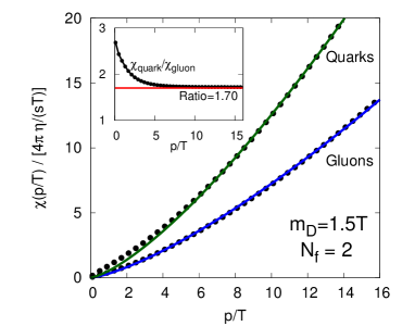
The results of the numerical solution of the Boltzmann equation for the two component case are shown as points in Fig. 6. The solid curves are the results of the fit done at intermediate momentum () with the result .
In order to solve for the two constants ( and ) we need two constrains. The first constraint relates the coefficients to the shear viscosity,
| (45) |
The sum is over quarks and gluons with degeneracies and . The second constraint comes from fixing the ratio of to the numerical solution of the Boltzmann equation. This ratio is shown in Fig. 6 and at large enough momentum () we find
| (46) |
The explicit computation of the two coefficients () in terms of the above ratio and is worked out in Appendix D.
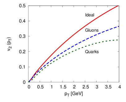
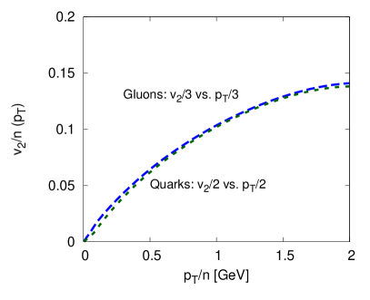
In Fig. 7 we show the elliptic flow of quarks and gluons. Note the larger suppression for quarks as the gluons are forced into equilibrium much quicker. This quicker relaxation can not simply be explained by naively assuming Casimir scaling, . Instead this ratio involves a playoff between the faster equilibration rate of gluons and the tendency of identity changing processes , , to equilibrate disequilibrium between the quarks and gluons. This ratio is evaluated analytically at asymptotically large momentum in Appendix C.
The distinct quark and gluon elliptic flow is completely due to the different viscous corrections, which in turn is related to the different relaxation rates of quarks and gluons. Let us note that if we scale both the and of gluons by three and quarks by two, the result is a “universal curve” as shown in the right plot of Fig. 7. The observed scaling is completely accidental, but it led us to consider the possibility of finding similar scaling behavior in a meson / baryon system due to differences in the relaxation rates. This is discussed in detail in the next section.
IV.2 Two component meson/baryon gas
The QCD matter immediately before freezeout is certainly not a weakly coupled quark-gluon plasma, but it might be described as a hadron (resonance) gas. Just as for the quarks and gluons, there is no reason to think that the mesons and baryons should show the same efficiency in equilibrating. But rather than claim a specific model for the partially equilibrated state of such a system, we will just do some phenomenology to see how different thermalization rates could affect the observed species-dependent elliptic flow behavior. To study the hydrodynamics of this system we switch from the Ideal gas equation of state to a lattice motivated Laine:2006cp . Further details of the simulation are presented in Appendix A.
We consider a meson / baryon gas whereby mesons and baryons have the off-equilibrium corrections and respectively,
| (47) |
We assume both species have the same power-law correction to spectra,
| (48) |
but we allow for different coefficients () which we will choose in order to give reasonable agreement with data. For simplicity, we will consider two different Ansätze: quadratic () and radiative (), and take the following ratios which, as we will show, fit the data rather well:
| (51) |
Finally, the numerical values of the coefficients can be identified with the shear viscosity through
| (52) |
where the sum extends over all mesons/baryons having GeV respectively. This choice reproduces the lattice parametrization of the equation of state below MeV. We find the following values for the coefficients at our freeze-out temperature of MeV,
| (55) | |||
| (58) |
Before computing particle spectra we would like to make an aside about the way elliptic flow is computed. By definition is given by
| (59) |
where is short for and is the first viscous correction to this. In the above expression the viscous correction to the phase space distribution, , occurs both in the numerator as well as in the normalization from the denominator. Since we have restricted the viscous correction to be linear in gradients of field quantities we should therefore require that be computed to the same order. We therefore expand the denominator
| (60) |
so the expression retains terms to first order in only. In the following we will show both the expanded and unexpanded expressions for , shading the region between the two results in order to give an estimate for the uncertainty in the gradient expansion. The upper limit of the band corresponds to Eq. (59) while the lower limit is Eq. (60). In figures where the uncertainty band is omitted the plotted curve corresponds to Eq. (59).
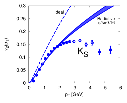
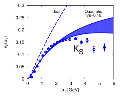
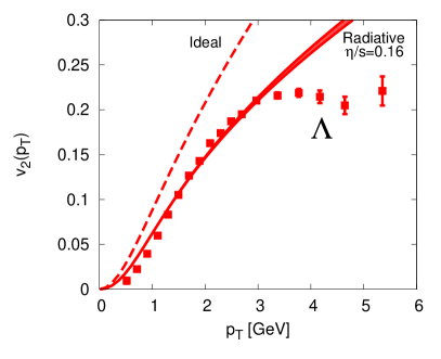
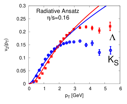
Let us now discuss how the different Ansätze fare with the experimental data. We have chosen in order to give reasonable agreement with the data in the transverse momentum range . The spectra for and are presented in Fig. 8 using either the radiative () or quadratic () Ansatz. For GeV we find good agreement between the viscous hydrodynamic results and data. If one included hadronic rescattering the low momentum component of the would be pushed out towards higher giving better agreement with the data. Above 2-3 GeV large differences between the radiative and quadratic Ansätze are realized. We must warn that at higher one cannot make a direct comparison with data since a larger fraction of the yield will come from fragmenting partons, which have not been included. In addition, the hydrodynamic description starts to break down at larger . Regardless, one must keep in mind that for large enough momentum ( i.e. GeV) the two Ansätze used here are clearly discernible and the choice of Ansatz could in principle lead to differences in the extracted viscosity.
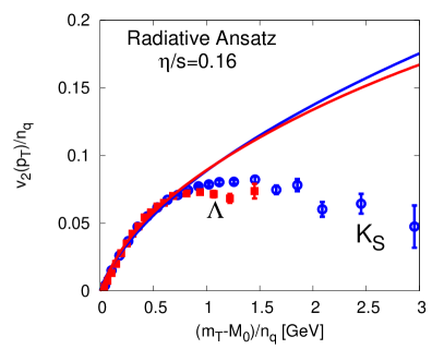
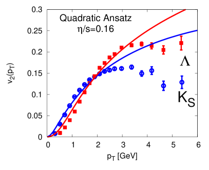
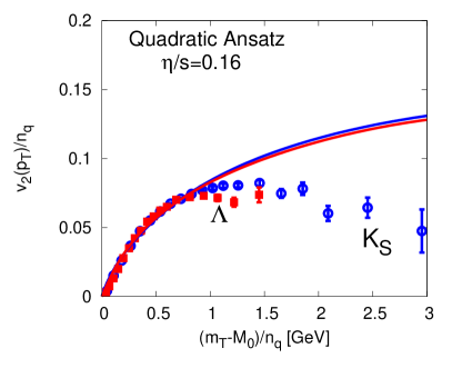
We would now like to investigate whether we observe a meson / baryon scaling, similar to the accidental quark / gluon scaling we found from first principles earlier. For clarity, we again present the above results with mesons and baryons on the same figure. This is shown for both radiative and quadratic Ansätze in Fig. 9. The figures show the corresponding results with both and re-scaled by the number of constituent quarks. The scaling of the data is the well-known phenomenon of constituent quark scaling. We find that viscous hydrodynamics reproduces this “universal curve” as well. This is due to the difference in relaxation rates between mesons and baryons, which was treated as a free parameter. The possible microscopic origin of this ratio is discussed further in Section V.
We should also point out that this relaxation time scaling is fairly robust to changes in the equation of state. While changing the equation of state will clearly affect the behavior, these changes will only have modest modifications to the viscous correction to the distribution functions. The qualitative feature that species with smaller relaxation times have a stronger elliptic flow is borne out by Fig. 7 (a quark gluon plasma equation of state) and Fig. 9 (a lattice equation of state). Further study of the equation of state is left to future work.
V Summary and Discussion
In this work we have presented a systematic study of the first viscous correction to the thermal distribution function. All simulations of viscous hydrodynamics so far have used the quadratic Ansatz
| (61) |
but this is only an educated guess.
First we studied the form of (or ) in a momentum dependent relaxation time approximation and derived a simple formula
| (62) |
Examining this formula we considered two special cases (where the equilibration time is proportional to energy) and (where the equilibration time is independent of energy). These give rise to quadratic () and linear () dependence on momentum, as is summarized in Table 1. We expect that, provided QCD is describable in terms of quasi-particles, the first viscous correction should lie between these cases. Fig. 2 compares these two extreme limits for the functional form of the viscous correction. It is important to emphasize that the two simulations have precisely the same shear viscosity. Comparing our results for the elliptic flow in these two theories, we see that the integrated elliptic flow is largely determined by the shear viscosity, while differential quantities such as at high depend on the equilibration rates at high momentum. The integrated elliptic flow is determined to a large extent by the hydrodynamic variables . (An explicit formula relating to and is given in Teaney:2009qa which in turn was motivated by earlier observations KSH ; Ollitrault:1992bk ; Romatschke:2007mq ; Dusling:2007gi . )
| Model | Physics | Formula |
| Relaxation time, | Relaxation time grows with particle momentum. | |
| Relaxation time , | Relaxation time independent of momentum. | |
| Scalar theory | Randomizing collisions which happen rarely | |
| QCD Soft Scatt. | Soft collisions lead to a random walk of hard particles. | |
| QCD Hard Scatt. | Hard collisions lead to a random walk of hard particles. | |
| QCD Rad. E-loss | Radiative energy controls the approach to equilibrium. In the LPM regime controls the radiation rate. |
The quadratic ansatz is valid only for fairly specialized theories. For instance, examining Table 1 we see that scalar theories follow this Ansatz. The reason is that the cross-section falls as , so higher-energy particles see a more transparent medium and equilibrate more slowly.
For different reasons the quadratic Ansatz is also valid in a soft scattering approximation to high temperature QCD (see Row 4 of Table 1). In this limit, which treats as an expansion parameter, soft collisions lead to the momentum diffusion and drag of hard gluons. If the momentum diffusion is independent of particle energy and the drag is constant, we get the quadratic Ansatz. If the momentum diffusion increases logarithmically with particle energy, we find a logarithmic correction to this Ansatz (see Row 5 of Table 1). A formula which summarizes the asymptotic form of both of these cases is
| (63) |
where is the rate is energy loss of a particle with momentum (see Eq. (28) and Eq. (34) for explicit formulas in certain limits).
However, the effect of bremsstrahlung completely changes this picture. A naive (Bethe-Heitler) treatment of radiative energy loss would lead to a relaxation rate independent of momentum, but including the LPM effect, the viscous correction behaves asymptotically as
| (64) |
This formula is summarized in Row 6 of Table 1 and provides a concrete connection between viscous corrections and radiative energy loss which is further explored in Fig. 5 and surrounding text.
From a phenomenological perspective, the LPM effect is not entirely dominant and collisions are important in the relevant momentum range. A phenomenological fit to numerical results for the first viscous correction, including both collisions and collinear radiation without making the strict LPM approximation, shows that the first viscous correction is reasonably well described by the following phenomenological form:
| (65) |
Fig. 4 compares this functional form to the linear and quadratic Ansätze motivated by the relaxation time approximation. We see that the general expectation from high temperature QCD is that in the relevant momentum range the first viscous correction is slightly closer to the linear rather than the quadratic ansatz.
We next studied two component plasma starting with a two component plasma of quarks and gluons. Since the relaxation rates of the quarks and gluons are not the same the two components do not have the same distribution function. At high momentum an analysis of collinear splittings , , shows that both the quark and gluon distribution behave as . However the ratio of the quark and gluon viscous corrections approaches a constant
| (66) |
The constant is determined by the ratio of Casimirs and the dynamics of the QCD splitting functions. It also depends weakly on the number of quark flavors and we have quoted the two flavor case.
Motivated by this example, we have postulated that the baryon and meson components of the medium have different equilibration rates. Indeed, there is no reason to expect that these species would equilibrate at the same rate. Then we fitted (by eye) the ratio of relaxation rates to reproduce the baryon and meson elliptic flows. If the ratio of relaxation times is
| (67) |
meaning that baryons relax to equilibrium 1.5 times faster than mesons, then the resulting viscous hydrodynamic calculation effortlessly reproduces the universal “constituent quark scaling” curve. Physically what is happening is that in ideal hydrodynamics the baryons and mesons have approximately the same elliptic flow which is approximately described by a linear rise in . The viscous correction then dictates that the baryons will follow this ideal trend 1.5 times farther than the mesons. Although it is not obvious from the data shown in Fig. 9, the data do not show scaling above , i.e. the last Lambda point is a fluctuation upward (This is seen quite clearly in recent PHENIX dataPHENIXv2a ; PHENIXv2b .) It is interesting that the data also deviate from hydrodynamic predictions above this point.
It is tempting to speculate as to the microscopic origin of the factor of . The baryons and mesons in the region are produced in the complex transition region where the energy density decreases from to . In this range, the temperature decreases by only . However, the hydrodynamic simulations evolve this complicated region for a significant period of time, , and the hadronic currents are built up over this time period. The interactions are probably quite inelastic and are not easily classified as hadronic or partonic in nature. The additive quark model was used to describe high energy total cross sections which are similarly inelastic AQM . It predicts the ratio of high energy nucleon-nucleon to pion-nucleon (as well as pion-nucleon to pion-pion) cross sections to be in reasonable agreement with the experimental ratio. Perhaps similar physics is responsible for the different baryon and meson elliptic flows. In fact, the splitting of the baryonic and mesonic elliptic flows was predicted at least qualitatively by UrQMD which implements the additive quark model Bleicher:2000sx . On the other hand, the factor of in the relative relaxation times could be simply a combination of dynamical and group theoretical factors of accidental significance.
In summary, a species dependent relaxation time provides a coherent and physically transparent explanation for the complicated trends observed in the elliptic flow data measured at RHIC.
Acknowledgments
KD is supported by the US-DOE grant DE-AC02-98CH10886. DT would like to thank Paul Sorenson, Raimond Snellings, and Jiangyong Jia for informative discussions. DT is supported in part by an OJI grant from the US Department of Energy DE-FG-02-08ER4154 and the Sloan Foundation. GM would like to thank Paul Romatschke for useful conversations, the physics department at the Universidad Autonoma Madrid for hospitality while this work was completed, and the Alexander von Humboldt Foundation for its support through a F. B. Bessel prize. GM’s work was supported in part by the Natural Sciences and Engineering Research Council of Canada.
Appendix A Details of hydrodynamic description
The initial condition of the hydrodynamic evolution is set by a Glauber model and the energy density is proportional to the number of binary collisions. More specifically we take
| (68) |
where is the energy per binary collision and mb is the inelastic nucleon-nucleon cross section.
In this work we will use the following evolution equation for ,
| (69) |
which is identical to the stress tensor used in Dusling:2007gi . Other possibilities are also possible Dusling:2009zz which will not change the results of this work on a qualitative level. In the above expression is the vorticity and . There is one technical detail that warrants discussion. At large transverse distances the viscous pressure tends to become larger than the ideal pressure and the equations become unstable. It is therefore necessary to cutoff our auxiliary tensor when it becomes large. More precisely we take
| (70) |
where and .
In the first part of this paper we consider an ideal gas equation of state, . For a two flavor QGP the ideal Stefan Boltzmann gas gives , which roughly corresponds to the relation found on the lattice. (For the highest temperatures in the simulation it is above this value and for the lowest temperatures in the simulation it is this value). We have decided to use the same ratio for both the gluon gas and quark + glue simulations in order to get the fairest possible phenomenological estimate for the size of the viscous corrections in a realistic heavy ion event.
For simulations using the ideal gas EoS the freeze-out contour is taken at constant GeV/fm3 corresponding to a temperature of 140 MeV. The default impact parameter is 7.6 fm and the shear viscosity to entropy ratio is .
In the second part of this paper where we compute spectra of a meson/baryon gas we have used a lattice motivated equation of state Laine:2006cp . In this case the freeze-out surface is set by GeV/fm3 corresponding to a temperature of 150 MeV. We have used a default impact parameter of 6.8 fm corresponding to a centrality class of 10-40% and a shear viscosity to entropy ratio of .
Appendix B Collision Integrals
In this section we will give the details leading to Eq. (26) for a scalar theory and Eq. (33) for pure glue.
B.1 Scalar theory
Our starting point is Eq. (24). Substituting the form specified in Eq. (25) into this equation yields in a Boltzmann approximation
| (71) | |||||
where is the Lorentz invariant extension777 Specifically, defining the projector onto the local rest frame , we have In the local rest frame implicit here, we have and for . of . The integrals over and are Lorentz covariant and can be performed by standard tricks; the term can be factored out, leading to , while the integral over must return a rank-2 tensor depending only on . There are only two such tensors, and contraction with and establishes that
| (72) |
The integral equation becomes
| (73) |
where we used that is traceless, . Performing the angular integration in the plasma frame, the terms integrate to zero; so does the term, because is traceless. Performing the trivial radial integration, we find Eq. (26).
B.2 Pure glue
Our goal here is to derive Eq. (33) and Eq. (34). Our starting point is the collision integral Eq. (23) with matrix elements given by Eq. (31)
| (74) |
Using the definition, , one can pull out the common factor, . The remaining integral on the right hand side (called ) must have the form since this is the only symmetric traceless tensor which can be constructed out of and . Straightforward analysis then shows that
where for instance
| (76) |
is the second Legendre polynomial.
We will evaluate this integral in a leading approximation. Asymptotically, the momenta and are large, while and are of order the temperature888We will discuss the region of phase space where is small. Since the particles are identical, there is also an equal contribution where is small, i.e. when and are large and and are of order . Our original definition of the transition rate includes a symmetry factor for the identical particle final state. To ease the discussion in this section, we will simply drop the symmetry factor and neglect -channel contribution. . In this limit we can make the Boltzmann approximation, , and can treat as close to . Specifically we take
| (77) |
and then write
| (78) |
We also note that and are close to and therefore and are small. Then we can write Eq. (B.2) as
| (79) |
where the average energy loss rate for a particle with momentum is
| (80) |
i.e. the energy loss is the transition rate weighted with the energy transfer. The energy loss to leading has been determined by Bjorken Bjorken:1982tu and Braaten and Thoma Braaten:1991jj and reads
| (81) |
One can verify that when terms suppressed by are dropped we have
| (82) |
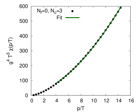
Fig. 10 shows a fit based on Eq. (82) which does a reasonable job in reproducing our numerical results at high momentum.
For completeness we will rederive Eq. (81). In order to evaluate the phase space integrals over we use the “t-channel parametrization” of Arnold:2003zc . Following the logic that leads from (A.14) to (A.21) of this work, we write the phase space as
| (83) |
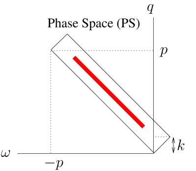
where the momentum transfer is and the energy transfer is . The vector is taken along the axis and the vector lies in the plane. The angle is the azimuthal angle of with respect to the plane. The energy transfer and momentum transfer are restricted to the available phase space
| (84) | |||||
| (85) |
which is also exhibited in Fig. 11.
Using the definitions of the kinematic variables, the Mandelstam invariants are
| (86) | |||||
| (87) | |||||
| (88) |
To evaluate the collision integral, we are to substitute these expressions for the Mandelstam invariants into the matrix elements and perform the integrals over the phase space. Close inspection of the result of this procedure shows how comes about. First, the logarithm comes from integrating over the phase space region where and as shown by the band shown in Fig. 11. Since the integral is over the interval, , the phase-space integral is approximately
| (89) |
and we may neglect the stimulation factor, . Second, only the highest powers of and contribute to the ultraviolet logarithm. The integrated matrix elements with these restrictions is
| (90) |
Then the total total transition rate is
| (91) |
Performing the integral over , we arrive at the result quoted in Eq. (81).
Appendix C Viscous distribution function and
In this appendix we derive the form of the viscous distribution function for asymptotically large momenta. In doing this we will relate the high tail of the distribution function with the energy loss parameter .
The starting point is the Boltzmann equation containing near collinear splitting processes. We neglect processes as these will be sub-leading at large momenta. Therefore
| (92) |
where
| (93) |
In the above expression is the distribution function of species . The degeneracy factor, is 16 for gluons and for quarks.
Now linearize the collision integral
| (94) |
Doing the integral over and expanding out the LHS in the typical way we get
| (95) |
Then note at very high momentum
| (96) |
Let us now consider a two component plasma of quarks and gluons. Using the Ansatz we are left with
| (97) |
The splitting functions at leading log order are
| (98) | |||||
The behavior here together with the behavior explicitly on the RHS of Eq. (C) must cancel the behavior on the LHS of Eq. (C). This fixes or , so . This proves the claim in the main text that the asymptotic behavior should be .
For a gluon gas we find
| (99) |
and
| (100) |
For a two-flavor quark-gluon gas we find
| (101) |
The ratio is
| (102) |
not too different from the ratio we found by fitting. This ratio depends on . For 1 flavor it is 1.702, for 3 flavors it is 1.618, and in the limit of infinite flavors it approaches 1.128. This diminishing ratio occurs because, at larger , more and more splitting processes are and , which equilibrate the numbers of quarks and gluons towards each other.
Appendix D Two component system
In this appendix we derive relationships between the off-equilibrium distribution function, and the shear viscosity of a two component system.
We consider a gas of bosons and fermions as it will have applications to a gas of quarks and gluons or a gas of mesons and baryons.
| (103) |
The off-equilibrium correction takes the form
| (104) |
The goal is to find values of the coefficients and as a function of and .
First we define the partial viscosity of each species
| (105) |
which will yield a total viscosity of
| (106) |
For massive particles the phase space integrals must be done numerically, but for massless particles, integrating Eq. (105) yields
| (107) |
with . Let us define as the ratio of the partial viscosities,
| (108) |
Making use of the relations
| (109) |
we find
| (110) |
References
- (1) J. Adams et al. [STAR Collaboration], Nucl. Phys. A 757, 102 (2005) [arXiv:nucl-ex/0501009].
- (2) K. Adcox et al. [PHENIX Collaboration], Nucl. Phys. A 757, 184 (2005) [arXiv:nucl-ex/0410003].
- (3) B. B. Back et al., Nucl. Phys. A 757, 28 (2005) [arXiv:nucl-ex/0410022].
- (4) I. Arsene et al. [BRAHMS Collaboration], Nucl. Phys. A 757, 1 (2005) [arXiv:nucl-ex/0410020].
- (5) T. Hirano and Y. Nara, Nucl. Phys. A 743, 305 (2004). D. Teaney, J. Lauret and E. V. Shuryak, Phys. Rev. Lett. 86, 4783 (2001); ibid arXiv:nucl-th/0110037. P. F. Kolb, P. Huovinen, U. W. Heinz and H. Heiselberg, Phys. Lett. B 500, 232 (2001). P. Huovinen, P. F. Kolb, U. W. Heinz, P. V. Ruuskanen and S. A. Voloshin, Phys. Lett. B 503, 58 (2001). C. Nonaka and S. A. Bass, Phys. Rev. C 75, 014902 (2007).
- (6) B. I. Abelev et al. [STAR Collaboration], Phys. Rev. C 77, 054901 (2008) [arXiv:0801.3466 [nucl-ex]].
- (7) A. Adare et al. [PHENIX Collaboration], Phys. Rev. Lett. 98, 162301 (2007) [arXiv:nucl-ex/0608033].
- (8) See for example the recent review of coalesence and constituent quark scaling: P. Sorensen, arXiv:0905.0174 [nucl-ex], invited review for QGP4, editors R. C. Hwa and X. N. Wang.
- (9) Z. w. Lin and C. M. Ko, Phys. Rev. C 65, 034904 (2002) [arXiv:nucl-th/0108039].
- (10) D. Molnar and S. A. Voloshin, Phys. Rev. Lett. 91, 092301 (2003) [arXiv:nucl-th/0302014].
- (11) V. Greco, C. M. Ko and P. Levai, Phys. Rev. Lett. 90, 202302 (2003) [arXiv:nucl-th/0301093].
- (12) R. J. Fries, B. Muller, C. Nonaka and S. A. Bass, Phys. Rev. Lett. 90, 202303 (2003) [arXiv:nucl-th/0301087].
- (13) R. Baier and P. Romatschke, Eur. Phys. J. C 51, 677 (2007) [arXiv:nucl-th/0610108].
- (14) P. Romatschke, Eur. Phys. J. C 52, 203 (2007) [arXiv:nucl-th/0701032].
- (15) P. Romatschke and U. Romatschke, Phys. Rev. Lett. 99, 172301 (2007) [arXiv:0706.1522 [nucl-th]].
- (16) H. Song and U. W. Heinz, Phys. Lett. B 658, 279 (2008) [arXiv:0709.0742 [nucl-th]].
- (17) K. Dusling and D. Teaney, Phys. Rev. C 77, 034905 (2008) [arXiv:0710.5932 [nucl-th]].
- (18) P. Huovinen and D. Molnar, Phys. Rev. C 79, 014906 (2009) [arXiv:0808.0953 [nucl-th]].
- (19) H. Song and U. W. Heinz, Phys. Rev. C 77, 064901 (2008) [arXiv:0712.3715 [nucl-th]].
- (20) P. Bozek, Phys. Rev. C 77, 034911 (2008) [arXiv:0712.3498 [nucl-th]].
- (21) W. A. Hiscock and L. Lindblom, Annals Phys. 151, 466 (1983).
- (22) W. A. Hiscock and L. Lindblom, Phys. Rev. D 31, 725 (1985).
- (23) W. Israel, Ann. Phys. 100 (1976) 310; W. Israel and J.M. Stewart, Phys. Lett. 58A (1976) 213.
- (24) M. Grmela, H.C. Öttinger, Phys. Rev. E 56, 6620 (1997). H.C. Öttinger, M. Grmela, Phys. Rev. E 56, 6633 (1997). H.C. Öttinger, Phys. Rev. E 57, 1416 (1993).
- (25) H. C. Öttinger, Physica A 254 (1998) 433-450.
- (26) F. Cooper and G. Frye, Phys. Rev. D. 10, 186 (1974).
- (27) See for example, D. A. Teaney, arXiv:0905.2433 [nucl-th], invited review for QGP4, editors R. C. Hwa and X. N. Wang.
- (28) S. Jeon, Phys. Rev. D 52, 3591 (1995) [arXiv:hep-ph/9409250].
- (29) P. Arnold, G. D. Moore and L. G. Yaffe, JHEP 0111, 057 (2001) [arXiv:hep-ph/0109064].
- (30) P. Arnold, G. D. Moore and L. G. Yaffe, JHEP 0301, 030 (2003) [arXiv:hep-ph/0209353].
- (31) P. Arnold, G. D. Moore and L. G. Yaffe, JHEP 0011, 001 (2000) [arXiv:hep-ph/0010177].
- (32) J. Hong and D. Teaney, in preparation.
- (33) M. H. Thoma and M. Gyulassy, Nucl. Phys. A 544 (1992) 573C.
- (34) E. Braaten and M. H. Thoma, Phys. Rev. D 44, 1298 (1991); ibid. Phys. Rev. D 44, 2625 (1991).
- (35) P. Arnold, G. D. Moore and L. G. Yaffe, JHEP 0305, 051 (2003) [arXiv:hep-ph/0302165].
- (36) J. D. Bjorken, FERMILAB-PUB-82-059-THY.
- (37) G. Baym, H. Monien, C. J. Pethick and D. G. Ravenhall, Phys. Rev. Lett. 64, 1867 (1990).
- (38) H. Heiselberg, Phys. Rev. D 49, 4739 (1994) [arXiv:hep-ph/9401309].
- (39) R. Baier, Y. L. Dokshitzer, A. H. Mueller, S. Peigne and D. Schiff, Nucl. Phys. B 483, 291 (1997) [arXiv:hep-ph/9607355].
- (40) R. Baier, Y. L. Dokshitzer, A. H. Mueller, S. Peigne and D. Schiff, Nucl. Phys. B 484, 265 (1997) [arXiv:hep-ph/9608322].
- (41) P. Arnold, G. D. Moore and L. G. Yaffe, JHEP 0206, 030 (2002) [arXiv:hep-ph/0204343].
- (42) P. Arnold and C. Dogan, Phys. Rev. D 78, 065008 (2008) [arXiv:0804.3359 [hep-ph]].
- (43) S. A. Bass, C. Gale, A. Majumder, C. Nonaka, G. Y. Qin, T. Renk and J. Ruppert, Phys. Rev. C 79, 024901 (2009) [arXiv:0808.0908 [nucl-th]].
- (44) X. f. Guo and X. N. Wang, Phys. Rev. Lett. 85, 3591 (2000). X. N. Wang and X. f. Guo, Nucl. Phys. A 696, 788 (2001). B. W. Zhang and X. N. Wang, Nucl. Phys. A 720, 429 (2003). A. Majumder, E. Wang and X. N. Wang, Phys. Rev. Lett. 99, 152301 (2007). A. Majumder and B. Muller, Phys. Rev. C 77, 054903 (2008). A. Majumder, R. J. Fries and B. Muller, Phys. Rev. C 77, 065209 (2008).
- (45) S. Jeon and G. D. Moore, Phys. Rev. C 71, 034901 (2005)
- (46) B. G. Zakharov, JETP Lett. 63, 952 (1996), hep-ph/9607440. B. G. Zakharov, JETP Lett. 65, 615 (1997), hep-ph/9704255. B. G. Zakharov, Phys. Atom. Nucl. 61, 838 (1998), hep-ph/9807540. C. A. Salgado and U. A. Wiedemann, Phys. Rev. D68, 014008 (2003), hep-ph/0302184. U. A. Wiedemann, Nucl. Phys. B582, 409 (2000), hep-ph/0003021. U. A. Wiedemann, Nucl. Phys. B588, 303 (2000), hep-ph/0005129. C. A. Salgado and U. A. Wiedemann, Phys. Rev. Lett. 89, 092303 (2002), hep-ph/0204221. N. Armesto, C. A. Salgado, and U. A.Wiedemann, Phys. Rev. Lett. 94, 022002 (2005), hep-ph/0407018.
- (47) M. Laine and Y. Schroder, Phys. Rev. D 73, 085009 (2006) [arXiv:hep-ph/0603048].
- (48) Arkadij Taranenko for the PHENIX Collaboration, presented at Quark Matter 2009, Knoxville, Tennessee, March 30–April 4 (2009).
- (49) S. Huang [PHENIX Collaboration], J. Phys. G 36 (2009) 064061.
- (50) P. F. Kolb, J. Sollfrank, and U. Heinz, Phys. Rev. C 65, 054909 (2000).
- (51) J. Y. Ollitrault, Phys. Rev. D 46, 229 (1992).
- (52) E. M. Levin and L. L. Frankfurt, Pisma ZhETP, 3, 105 (1965). H. J. Lipkin and F. Sheck, Phys. Rev. Lett. 16, 71 (1966).
- (53) M. Bleicher and H. Stoecker, Phys. Lett. B 526, 309 (2002) [arXiv:hep-ph/0006147].
- (54) K. Dusling, Acta Phys. Polon. B 40, 963 (2009).