Particle diode: Rectification of interacting Brownian ratchets

Abstract

Transport of Brownian particles interacting with each other via the Morse potential is investigated in the presence of an ac driving force applied locally at one end of the chain. By using numerical simulations, we find that the system can behave as a particle diode for both overdamped and underdamped cases. For low frequencies, the transport from the free end to the ac acting end is prohibited, while the transport from the ac acting end to the free end is permitted. However, the polarity of the particle diode will reverse for medium frequencies. There exists an optimal value of the well depth of the interaction potential at which the average velocity takes its maximum. The average velocity $\upsilon$ decreases monotonically with the system size $N$ by a power law $\upsilon\propto N^{-1}$.

I Introduction

Brownian motors a1 , rectifying nonequilibrium random walks on asymmetric potentials, have recently been proposed for a variety of applications, including in biological systemsa2 , as well as their potential technological applications ranging from classical non-equilibrium modelsa3 to quantum systemsa4 . Ratchets have been proposed to model the unidirectional motion driven by zero-mean non-equilibrium fluctuations. Broadly speaking, ratchet devices fall into three categories depending on how the applied perturbation couples to the substrate asymmetry: rocking ratchetsa5 , flashing ratchetsa6 , and correlation ratchets a7 . Additionally, entropic ratchets, in which Brownian particles move in a confined structure, instead of a potential, were also extensively studied a8 .

In many physical situations, one deals with not a single Brownian particle, but rather the with arrays of a finite number of interacting particles, which are usually in a periodic potential and acted upon by some external force. There has been a lot of interest in recent years in the dynamics of interacting Brownian particles a9 ; a10 ; a11 ; a12 ; a13 ; a14 . The reason for this interest is twofold a15 . First, experiments have provided a wealth of information about the motion of individual colloidal particles. A system of interacting Brownian particles is the simplest model of a colloidal suspension. Second, interacting Brownian particles constitute the simplest model system, on which one can test techniques and approximations of nonequilibrium statistical mechanics. Many-particle systems may exhibit some features not found in the single-particle counterparts, such as phase transitions, spontaneous ratchet effects, and negative mobility a9 ; a10 ; a11 ; a12 ; a13 ; a14 . The interacting Brownian ratchets been proposed for a variety of applications, including molecular motors a2 , friction a16 , diffusion of dimers on surfaces a17 , diffusion of colloidal particles a18 , DNA translocation through a nanopore a19 , charge density waves a20 , and arrays of Josephson junctions a21 .

In the present work, we study the transport of Brownian particles interacting with each other via the Morse potential by applying an ac driving force at one end of the chain. From the numerical simulations, we find that the system can behave as a particle diode for both overdamped and underdamped cases, the transport is permitted when the ac driving force is applied at one end of the chain, while the transport is prohibited when the force acts on the other end of the chain.

II Model and Methods

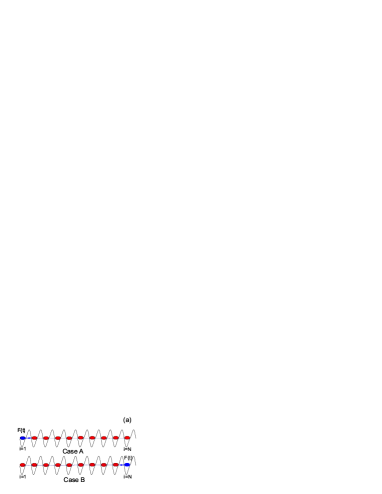
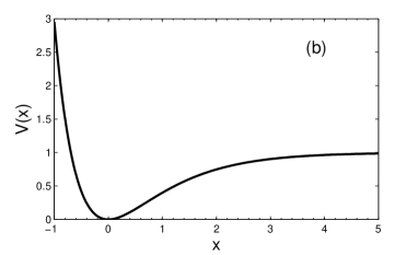
Figure 1: (Color online) (a) Schematic illustration of the model. Case A ($q=1$): the driving force acting on the left end. Case B ($q=N$): the driving force acting on the right end. The on-site potential $U(x)$ is asymmetric [shown in Eq. (7)]. The ac driving force $F(t)=A_{0}\sin(\omega t)$. $U_{0}=1.0$ and $\Delta=1.0$. Note that it is possible that two particles share a site or that the chain is torn apart. (b) The interaction potential $V(x)$ is a Morse potential [shown in Eq. (8)]. The interaction potential is asymmetric. The parameters are $k=1.0$ and $a=1.0$.

We consider an open system of $N$ point-like Brownian particles interacting with each other via the Morse potential $V$, with the substrate through the asymmetric periodic potential $U$. As to obtain the directed transport, a sustained time-periodical force $F(t)$ is applied at one end of the chain. The equations of motion for the underdamped case are

$$m\ddot{x}_{1}=f(x_{1})-G(x_{2}-x_{1})-\gamma\dot{x_{1}}+\xi_{1}(t)+\delta_{q,1}F(t),$$ (1)

$$m\ddot{x}_{i}=f(x_{i})+G(x_{i}-x_{i-1})-G(x_{i+1}-x_{i})-\gamma\dot{x_{i}}+\xi_{i}(t),$$ (2)

$$m\ddot{x}_{N}=f(x_{N})+G(x_{N}-x_{N-1})-\gamma\dot{x}_{N}+\xi_{N}(t)+\delta_{q,N}F(t),$$ (3)

where $x_{i}$ is the position of the $i$th particle, $m$ is the mass of the particles, and $N$ is total number of the particles. $f=-\frac{\partial U}{\partial x}$ and $G=-\frac{\partial V}{\partial x}$. $\gamma$ is friction coefficient and the noise terms $\xi_{i}(t)$ satisfy the fluctuation dissipation relations $\langle\xi_{i}(t)\xi_{i}(t^{{}^{\prime}})\rangle=2D\delta(t-t^{{}^{\prime}})$. $D$ is the noise intensity. The dot stands for the derivative with respect to time $t$. Where $q$ is a nature number. For $q=1$ and $q=N$, the ac driving force is applied at the left end and the right end, respectively.

When the inertia is negligible compared to the viscous damping, Eqs. (1)-(3) can be rewritten for overdamped case,

$$\gamma\dot{x_{1}}=f(x_{1})-G(x_{2}-x_{1})+\xi_{1}(t)+\delta_{q,1}F(t),$$ (4)

$$\gamma\dot{x_{i}}=f(x_{i})+G(x_{i}-x_{i-1})-G(x_{i+1}-x_{i})+\xi_{i}(t),$$ (5)

$$\gamma\dot{x}_{N}=f(x_{N})+G(x_{N}-x_{N-1})+\xi_{N}(t)+\delta_{q,N}F(t).$$ (6)

$U(x)$ is an asymmetrically periodic potential [shown in Fig. 1(a)]

$$U(x)=-U_{0}[\sin(x)+\frac{\Delta}{4}\sin(2x)],$$ (7)

where $U_{0}$ denotes the height of the potential and $\Delta$ is its asymmetry parameter.

The interaction potential between the nearest-neighbor particles is given by the Morse potential [shown in Fig. 1 (b)],

$$V(x)=k[1-\exp(-ax)]^{2},$$ (8)

where $k$ is well depth of the interaction potential and $a$ controls its width. The interaction potential is asymmetric and the repulsive force is dominating. $F(t)$ is a sustained time-periodical force,

$$F(t)=A_{0}\sin(\omega t),$$ (9)

where $A_{0}$ is the amplitude of the external force and $\omega$ is its frequency.

Here we mainly focus on the transport of the driven particles. The average velocity $\upsilon_{i}$ of the $i$th particle is,

$$\upsilon_{i}(t)=\lim_{t\rightarrow\infty}\frac{\langle x_{i}(t)-x_{i}(t_{0})\rangle}{t-t_{0}},$$ (10)

where $t_{0}$ and $t$ are the initial and the end times for the simulations, respectively. From Fig. 2 we can find that after the system reaches a stationary state, $\upsilon_{i}$ is independent of site position $i$. Therefore, we use the asymptotic velocity of the particle $N/2+1$ to measure the transport of the system $\upsilon=\upsilon_{N/2+1}$.

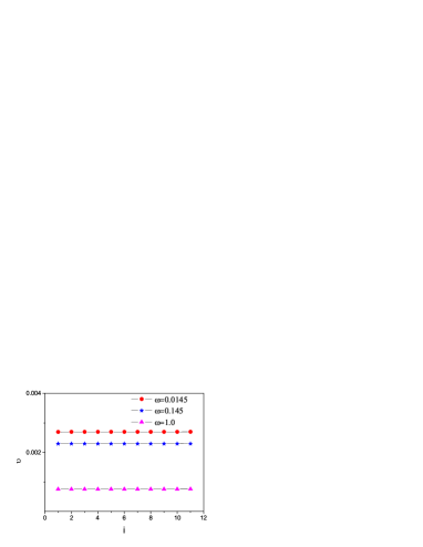
Figure 2: (Color online) The dependence of average velocity $\upsilon$ on the site $i$ for overdamped case. It is found that each particle has the same average velocity. The other parameters are $k=1.0$, $A_{0}=2.0$, $\Delta=1.0$, and $D=0.5$.

In our simulations, the equations of motion are integrated by using the second order Stochastic Runge-Kutta algorithmb1 with the small time step $\Delta t=10^{-3}$. All quantities of interest are averaged over 500 different realizations. The simulations are performed long enough to allow the system to reach a nonequilibrium steady state in which the local velocity is a constant along the chain. To obtain a steady state, the total integration is typically $10^{7}$ time units. We have checked that this is sufficient for the system to reach a steady state since the local velocity is independent of the site. For simplicity, we set $m=\gamma=U_{0}=a=1$.

III Numerical results and discussion

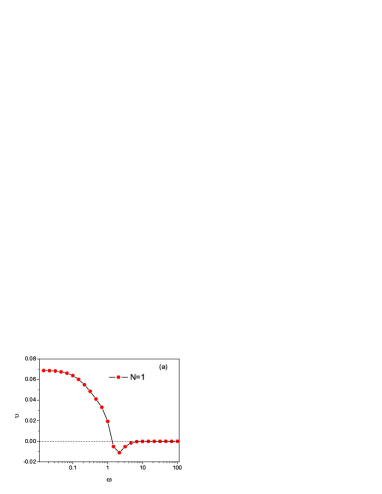
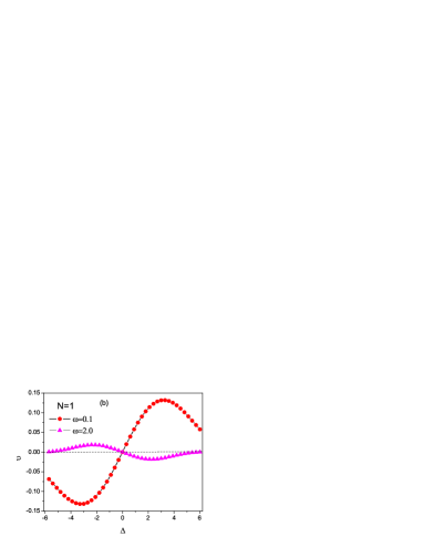
Figure 3: (Color online) Transport of overdamped Brownian particles for $N=1$. (a) Average velocity $\upsilon$ as a function of the driving frequency $\omega$; (b) Average velocity $\upsilon$ as a function of the asymmetry parameter $\Delta$ of the on-site potential for $\omega=0.1$ and $\omega=2.0$. The other parameters are $A_{0}=2.0$, $\Delta=1.0$, and $D=0.5$.

Figure 3 (a) shows the average velocity as a function of the driving frequency for overdamped case and $N=1$. The one-particle stochastic ratchets and stochastic resonance b2 ; b3 has been extensively studied. In the adiabatic limit $\omega\rightarrow 0$, the ac driving force can be expressed by two opposite forces $A_{0}$ and $-A_{0}$. The particles get enough time to cross both side from the minima of the potential. It is easier for particles to move toward the gentler slope side than toward the steeper side, so the average velocity is positive. As the frequency $\omega$ increases, due to the high frequency, the particles in one period have sufficient time to diffuse across the steeper side of the well, and therefore it leads to a negative average velocity. When the ac driving forces oscillate very fast $\omega\rightarrow\infty$, the particles will experience a time average constant force $F=\int_{0}^{\frac{2\pi}{\omega}}F(t)dt=0$, so the average velocity goes to zero. At some intermediate values of $\omega$, the average velocity crosses zero and subsequently reverse its direction. Figure 3 (b) depicts the average velocity as a function of the asymmetry parameter $\Delta$ for different frequencies. For the low frequency ($\omega=0.1$), the average velocity is negative for $\Delta<0$, zero at $\Delta=0,$ and positive for $\Delta>0$. However, for the medium frequency ($\omega=2.0$), one can obtain the opposite velocity, negative for $\Delta>0$ and positive for $\Delta<0$. Moreover, for both cases, there is an optimal value of $\Delta$ at which the velocity takes its extremal value. When $\Delta\rightarrow 0$, the system is absolutely symmetric and directed transport disappears. When $\Delta\rightarrow\infty$, the asymmetric potential described in Eq. (7) reduces to symmetric one with higher barriers, $U(x)=-\frac{U_{0}}{4}\Delta\sin(2x)$, resulting in zero velocity.

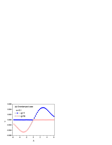
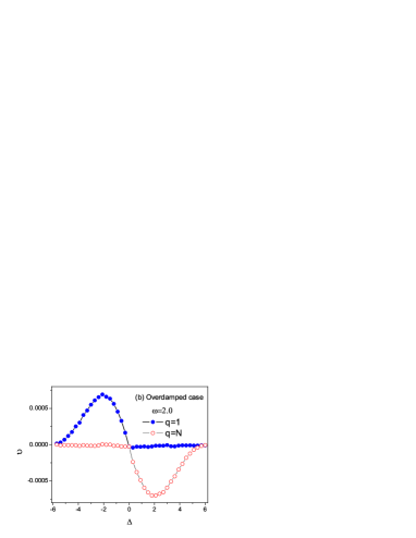
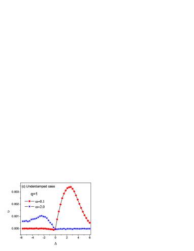
Figure 4: (Color online) Average velocity $\upsilon$ as a function of the asymmetry parameter $\Delta$ for $N>1$. (a) Overdamped case: $\omega=0.1$; (b) Overdamped case: $\omega=2.0$; (c) Underdamped case: $\omega=0.1$ and $\omega=2.0$. The other parameters are $k=1.0$, $A_{0}=2.0$, $N=11$, and $D=0.5$.

Now we will focus on finding how the interaction between the particles affects the directed transport for $N>1$. Figure 4 (a) depicts the dependence of the average velocity on the asymmetric parameter $\Delta$ for the low frequency ($\omega=0.1$). For case A ($q=1$), the ac force acting on the left end particle, the average velocity is positive for $\Delta>0$, it is easy for the particles to move from the left to the right and the system is a particle conductor. However, in the region $\Delta<0$, the average velocity is zero, the particle can not move from the right to the left and the system behaves as a particle insulator. For case B ($q=N$), the ac force acting on the right end particle, the transport from the left to the right is prohibited and the transport from the right to the left is permitted. The average velocity as a function of the asymmetry parameter $\Delta$ for the medium frequency ($\omega=2.0$) is shown in Fig. 4 (b). It is found that the unidirectional transport will also occur, but the direction of the velocity is opposite to that in Fig. 4 (a). From Figs. 4 (a) and 4 (b), we can conclude that the transport from the free end to the ac acting end is prohibited for low frequencies, while the transport from the ac acting end to the free end is cut off for medium frequencies. Therefore, the system behaves as a particle diode. We also found that the similar phenomena will occur for underdamped case shown in Fig. 4 (c).

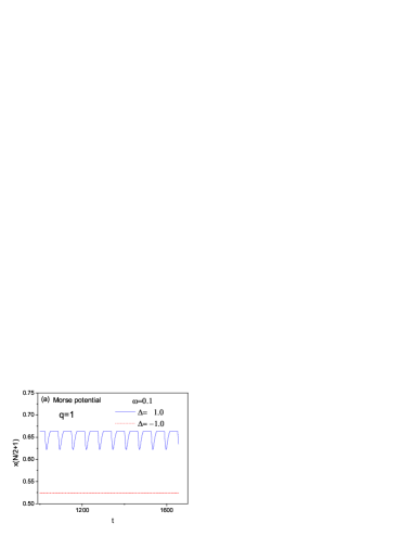
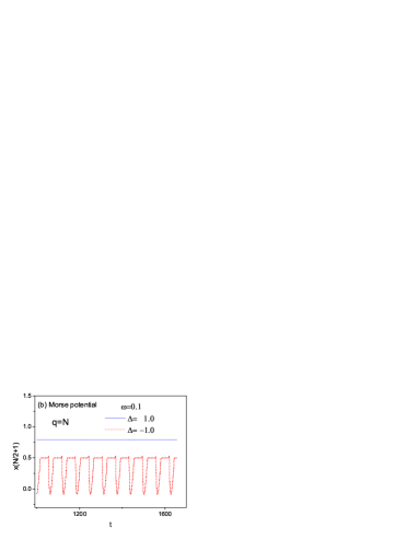
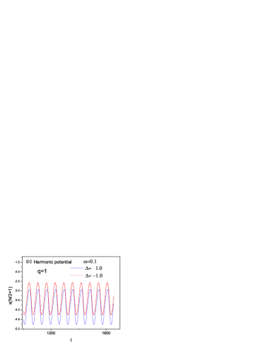
Figure 5: (Color online) Time dependent of the position of the central particle with zero noises ($D=0.0$) for overdamped case. (a) Morse potential and $q=1$; (b) Morse potential and $q=N$; (c) Harmonic potential and $q=1$. The other parameters are $N=11$, $\omega=0.1$, $A_{0}=2.0$, and $k=1.0$.

Note that the similar effects of the particle diode occur for the Lennard-Jones potential $V(x)=4k(\frac{1}{x^{12}}-2\frac{1}{x^{6}})$, where the repulsive force is dominated. However, the effects of the particle diode will disappear when the interaction potential is symmetric, for example, the Harmonic potential $V(x)=\frac{1}{2}kx^{2}$. In order to explain the unipolarity of the transport, we investigate the motion of the central particle with zero noises for low frequencies. For Morse potential and case A ($q=1$), we can find that the central particle behaves as a oscillator for $\Delta=1.0$. In this case, the driving force acting on the first particle can be transferred to the other particles. Therefore, directed transport will occur. However, the central particle is static for $\Delta=-1$, the central particle can not feel the driving force, so the transport is prohibited. For case B ($q=N$), where the driving force is applied at the last particle, the central particle is static for $\Delta=1.0$ and vibrates for $\Delta=-1.0$. Figure 5 (c) shows the movement of the central particle for Harmonic potential and case A. We can see that the central particle vibrates for both $\Delta=1.0$ and $\Delta=-1.0$, so the system can not behave as a particle diode. Therefore, the asymmetry of the transport originates from the asymmetry of the interaction potential.

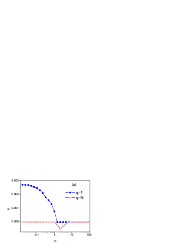
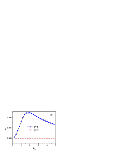
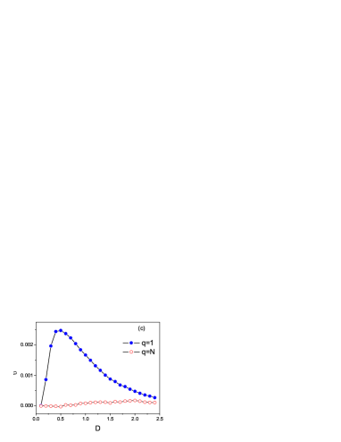
Figure 6: (Color online) Transport for overdamped case. (a) $\upsilon$ versus $\omega$ at $A_{0}=2.0$ and $D=0.5$; (b) $\upsilon$ versus $A_{0}$ at $D=0.5$ and $\omega=0.1$; (c) $\upsilon$ versus $D$ at $A_{0}=2.0$ and $\omega=0.1$. The other parameters are $N=11$, $\Delta=1.0$, and $k=1.0$.

Figure 6 (a) describes the average velocity as a function of the driving frequency for cases A ($q=1$) and B ($q=N$) at $\Delta=1.0$. For low frequencies, the transport is prohibited for case B. For medium frequencies, the average velocity is zero for case A. The average velocity for both cases A and B is always zero for the high frequencies. From Figs. 6 (b) and 6(c), we can see that the transport is prohibited for case B at $\Delta=1.0$ and $\omega=0.1$. For case A, there exists a value of $A_{0}$ at which the average velocity is maximal. When $A_{0}\rightarrow 0$, the ac driving force disappears, so the average velocity goes to zero. When $A_{0}\rightarrow\infty$, the driving force is very large and the effect of the potential will disappear, the average velocity tends to zero. Therefore, there is a peak in the curve of $\upsilon-A_{0}$. Similarly, the curve of $\upsilon-D$ shown in Fig. 6 (c) for case A is observed to be bell shaped. When $D\rightarrow 0$, the particles cannot pass across the barrier and there is no directed current. When $D\rightarrow\infty$ so that the noise is very large, the effect of the potential disappears and the average velocity tends to zero, also. Therefore, one can see that the curves demonstrate nonmonotonic behavior.

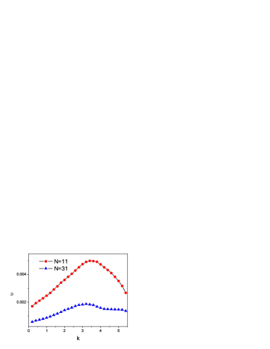
Figure 7: (Color online) Average velocity $\upsilon$ as a function of the well depth of the interaction potential $k$ for overdamped case. The other parameters are $\omega=0.1$, $A_{0}=2.0$, $\Delta=1.0$, and $D=0.5$.

The dependence of the average velocity on the well depth of the interaction potential is shown in Fig. 7 for overdamped case. When $k\rightarrow 0$, the interactions between the particles disappears, the central particle can not experience the ac driving force, the velocity goes to zero. When $k\rightarrow\infty$, the particles are strongly coupled, the interacting force is very large, the effect of the driving force will disappear, and the velocity also tends to zero. Therefore, there exists an optimal value of the well depth of the interaction potential at which the average velocity takes its maximum.

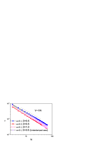
Figure 8: (Color online) Dependence of average velocity $\upsilon$ on the system size $N$ for different cases. For all cases the average velocity decrease in the form $\upsilon\propto N^{-1}$. The other parameter are $k=1.0$, $\Delta=1.0$, and $A_{0}=2.0$.

We show the system size dependence of the average velocity in Fig. 8 for different cases. It is clearly seen that the average velocity decreases monotonically with the system size $N$ for all cases. Remarkably, the average velocity decreases in power law $\upsilon\propto N^{-1}$. Note that the average velocity becomes to be independent of the system size when the driving force is applied at every particle of the chain.

Since the effect of rectification is very strong, it is necessary to give a theoretical analysis of the observed phenomenon by using some approximation. Here, we will focus on the small system with $N=3$, $D=0.2$ and $\omega=0.1$ for case A. The equations of motion for the two particles at $k=a=\gamma=1$ are

$$\dot{x_{1}}=\cos(x_{1})+\frac{\Delta}{2}\cos(2x_{1})-G(x_{2}-x_{1})+\xi_{1}(t)+A_{0}\sin(\omega t),$$ (11)

$$\dot{x_{2}}=\cos(x_{2})+\frac{\Delta}{2}\cos(2x_{2})+G(x_{2}-x_{1})-G(x_{3}-x_{2})+\xi_{2}(t),$$ (12)

$$\dot{x_{3}}=\cos(x_{3})+\frac{\Delta}{2}\cos(2x_{3})+G(x_{3}-x_{2})+\xi_{3}(t),$$ (13)

where $G(x)=-2\exp(-x)[1-\exp(-x)]$.

For case of $\Delta=1.0$, when the ac force acts on the left end, the particle $i=1$ will jump first, and we assume that the other particles are oscillating on average about the potential minima. Then, Eq. (11) can be approximately written

$$\dot{x_{1}}=\cos(x_{1})+\frac{\Delta}{2}\cos(2x_{1})-(\dot{x_{2}}+\dot{x_{3}})+\xi_{1}(t)+A_{0}\sin(\omega t),$$ (14)

the term $\dot{x_{2}}+\dot{x_{3}}$ is a random and does not dominate the transport. From this equation we can easily find that the particle $i=1$ will move towards the right on average. The distance between particle $i=1$ and $i=2$ is small and their interaction becomes strong. Then the particle $i=2$ can also jump and the ac driving force has been transferred from the particle $i=1$ to the particle $i=2$. Therefore, Eq. (12) can approximately become

$$\dot{x_{2}}=\cos(x_{2})+\frac{\Delta}{2}\cos(2x_{2})-\dot{x_{3}}+\mu\sin(\omega t)+\xi_{2}(t),$$ (15)

where $\mu$ is a constant. From Eq. (15), we can find that the particle $i=2$ will also move towards the right on average. Similarly, the distance between the particle $i=2$ and $i=3$ becomes small, and the ac force can be transferred to the particle $i=3$. The coupling terms prevent breaking the chain apart. Therefore, the three particles will move together to the right (see Fig. 9 (a)) and the particles $i=2$ and $3$ behave a collective movement.

However, for $\Delta=-1.0$, the average velocity based on Eq. (14) is negative and the particle $i=1$ will move to the left on average, the distance between the particle $i=1$ and $i=2$ becomes large. As we know, it is easy to pull the two particles apart for the Morse potential. The interaction will disappear quickly and the particles $i=2$ and $3$ can not feel the ac driving force from the particle $i=1$. Therefore, Eq. (12) can be approximately written

$$\dot{x_{2}}=\cos(x_{2})+\frac{\Delta}{2}\cos(2x_{2})-\dot{x_{3}}+\xi_{2}(t).$$ (16)

From Eq. (16), we can find that the particle $i=2$ behaves thermal equilibrium and no directed transport occurs. Therefore, the particle $i=1$ moves to the left on average and the particles $i=2$ and $3$ have zero average velocity (see Fig. 9 (b)). The ac driving force breaks the chain apart. If the ac driving can be transferred the other particles, the all particles can move together to the same direction. Due to the asymmetry of the Morse potential (it is easy to pull the particles apart), the ac driving can not be transferred to the other particle, the ac driving particle will escape from the chain and the chain is broken apart.

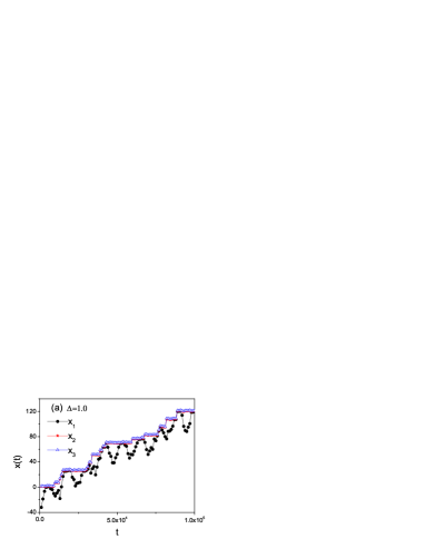
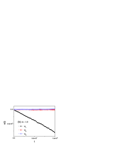
Figure 9: (Color online) The snapshots of the particles $i=1$, $2$, and $3$ for different cases. (a) $\Delta=1.0$; (b) $\Delta=-1.0$. The other parameters are $k=1$, $a=1$, $A_{0}=2.0$, $\omega=0.1$, and $D=0.2$.

IV Concluding Remarks

In conclusion, we study the directed transport of interacting Brownian particles by applying an ac driving force at one end of the chain. From the Brownian dynamic numerical simulations, we obtain the average velocity of the system for both overdamped and underdamped cases. One can observe some features not found in the single-particle counterparts, for example, the unipolarity of the transport. When the low frequency driving force is applied at the left end particle ($q=1$), the average velocity is positive for $\Delta>0$, the particles can easily move from the left the right and the system works as a particle conductor. However, for $\Delta<0$, the transport is prohibited, the particle can not move from the right to the left and the system behaves as a particle insulator. When the low frequency driving force is applied at the right end particle ($q=N$), the transport from the left to the right is prohibited and the transport from the right to the left is permitted. However, the direction of the transport for the medium frequency force is opposite to that for the low frequency force. We can call this system with the unidirectional transport as the particle diode. The unipolarity of the transport is caused by the asymmetry of the interaction potential. This asymmetry of the transport will disappear in the symmetry interaction potential, for example, Harmonic potential. In addition, it is also found that there exists an optimal value of the well depth $k$ at which the average velocity is maximal. The average velocity $\upsilon$ decreases monotonically with the system size $N$, $\upsilon\propto N^{-1}$.

This work was supported in part by the National Natural Science Foundation of China (Grants No. 61072029, No. 11004082, and No. 10947166) and the Guangdong Provincial Natural Science Foundation (Grants No. 01000025 and No. 01005249). Y. -f. H. also acknowledges the Natural Science Foundation of Hebei Province of China (Grant No. A2011201006).

References

- (1) P. Hänggi and F. Marchesoni, Rev. Mod. Phys. 81, 387 (2009); P. Reimann, Phys. Rep. 361, 57 (2002).
- (2) F. Julicher A. Adjari, and J. Prost, Rev. Mod. Phys. 69, 1269 (1997).
- (3) J. Rousselet, L. Salome, A. Adjari, and J. Prost, Nature 370, 446 (1994); L. P. Faucheux, L. S. Bourdieu, P. D. Kaplan, and A. J. Libchaber, Phys. Rev. Lett. 74, 1504 (1995).
- (4) C. S. Lee, B. Janko, I. Derenyi, and A. L. Barabasi, Nature 400, 337 (1999); I. Derenyi, C. S. Lee, and A. L. Barabasi, Phys. Rev. Lett. 80,1473 (1998); F. Marchesoni, Phys. Rev. Lett. 77, 2364(1996).
- (5) R. Bartussek, P. Hänggi, and J. G. Kissner, Europhys. Lett. 28, 459 (1994); M. O. Magnasco, Phys. Rev. Lett. 71, 1477 (1993).
- (6) P. Reimann, Phys. Rep. 290, 149 (1997); J. D. Bao and Y. Z. Zhuo, Phys. Lett. A 239, 228 (1998);P. Reimann, R. Bartussek, R. Haussler, and P. Hänggi, Phys. Lett. A 215, 26 (1996); B. Q. Ai, L. Q. Wang, and L. G. Liu, Chaos, Solitons Fractals 34, 1265 (2007).
- (7) C. R. Doering, W. Horsthemke, and J. Riordan, Phys. Rev. Lett. 72, 2984 (1994); R. Bartussek, P. Reimann, and P. Hänggi, Phys. Rev. Lett. 76, 1166 (1996).
- (8) B. Q. Ai and L. G. Liu, Phys. Rev. E 74, 051114 (2006); B. Q. Ai, Phys. Rev. E 80, 011113 (2009); F. Marchesoni, S. Savel’ev, Phys. Rev. E 80, 011120 (2009); B. Q. Ai, J. Chem. Phys. 131, 054111 (2009).
- (9) Z. G. Zheng, G. Hu, and B. Hu, Phys. Rev. Lett. 86, 2273 (2001).
- (10) I. Derenyi and T. Vicsek, Phys. Rev. Lett. 75, 374 (1995); F. Julicher and J. Prost, Phys. Rev. Lett. 75, 2618 (1995); Z. Csahok, F. Family, and T. Vicsek, Phys. Rev. E 55, 5179 (1997); A. Igarashi, S. Tsukamoto, and H. Goko, Phys. Rev. E 64, 051908 (2001).
- (11) S. Savel ev, F. Marchesoni, and F. Nori, Phys. Rev. Lett. 91, 010601 (2003); S. Savel ev, F. Marchesoni, A. Taloni, and F. Nori, Phys. Rev. E 74, 021119 (2006); S. Savel ev, F. Marchesoni, and F. Nori, Phys. Rev. E 71, 011107 (2005); S. Savel ev, F. Marchesoni, and F. Nori, Phys. Rev. E 70, 061107 (2004).
- (12) Jose Eduardo de Oliveira Rodrigues and R. Dickman, Phys. Rev. E 81, 061108 (2010); W. J. Nie, Q. H. Liao, and J. Z. He, Phys. Rev. E 82, 041130 (2010).
- (13) M. Kruger and M. Fuchs, Phys. Rev. E 81, 011408 (2010); M. Evstigneev, S. von Gehlen, and P. Reimann, Phys. Rev. E 79, 011116 (2009); P. Reimann, R. Kawai, C. Van Den Broeck, and P. Hanggi, Europhys. Lett. 45, 545 (1999).
- (14) R. M. da Silva, C. C. de Souza Silva, and S. Coutinho, Phys. Rev. E 78, 061131 (2008); A. D. Chepelianskii, M. V. Entin, L. I. Magarill, and D. L. Shepelyansky, Phys. Rev. E 78, 041127 (2008).
- (15) G. Szamel, J. Chem. Phys. 127, 084515 (2007).
- (16) A. E. Filippov, J. Klafter, and M. Urbakh, Phys. Rev. Lett. 92, 135503 (2004); F. Family, H. G. E. Hentschel, and Y. Braiman, J. Phys. Chem. B 104, 3984 (2000).
- (17) E. Heinsalu, M. Patriarca, and F. Marchesoni, Phys. Rev. E 77, 021129 (2008); X. R. Qin, B. S. Swartzentruber, and M. G. Lagally, Phys. Rev. Lett. 85, 3660 (2000).
- (18) C. Lutz, M. Kollmann, and C. Bechinger, Phys. Rev. Lett. 93, 026001 (2004).
- (19) K. Luo, T. Ala-Nissila, S.-C. Ying, and A. Bhattacharya, Phys. Rev. Lett. 100, 058101 (2008)
- (20) L. L. Bonilla, Phys. Rev. B 35, 3637 (1987).
- (21) H. S. J. van der Zant, T. P. Orlando, S. Watanabe, and S. H. Strogatz, Phys. Rev. Lett. 74, 174 (1995).
- (22) R. L. Honeycutt, Phys. Rev. A 45, 600 (1992).
- (23) V. N. Smelyanskiy, M. I. Dykman and B. Golding, Phys. Rev. Lett.82, 3193 (1999); M.I. Dykman, H. Rabitz, V. N. Smelyanskiy, B.E. Vugmeister, Phys. Rev. Lett.79, 1178 (1997); V. N. Smelyanskiy, M. I. Dykman, H. Rabitz, and B. E. Vugmeister, Phys. Rev. Lett. 79, 3113(1997).
- (24) D. G. Luchinsky, M. J. Greenall, P. V. E. McClintock, Phys. Lett. A 273, 316 (2000).