Simulating elliptic flow with viscous hydrodynamics

Abstract

In this work we simulate a viscous hydrodynamical model of non-central Au-Au collisions in 2+1 dimensions, assuming longitudinal boost invariance. The model fluid equations were proposed by Öttinger and Grmela OG . Freezeout is signaled when the viscous corrections become large relative to the ideal terms. Then viscous corrections to the transverse momentum and differential elliptic flow spectra are calculated. When viscous corrections to the thermal distribution function are not included, the effects of viscosity on elliptic flow are modest. However, when these corrections are included, the elliptic flow is strongly modified at large $p_{T}$. We also investigate the stability of the viscous results by comparing the non-ideal components of the stress tensor ($\pi^{ij}$) and their influence on the $v_{2}$ spectrum to the expectation of the Navier-Stokes equations ($\pi^{ij}=-\eta\left\langle\partial_{i}u_{j}\right\rangle$). We argue that when the stress tensor deviates from the Navier-Stokes form the dissipative corrections to spectra are too large for a hydrodynamic description to be reliable. For typical RHIC initial conditions this happens for $\eta/s\mbox{~{}{\raisebox{1.72218pt}{$>$}} {\raisebox{-2.58334pt}{$\sim$}}~{}}0.3$.

I Introduction

I.1 Motivation

One of the first and most exciting observations from the Relativistic Heavy Ion Collider (RHIC) was the very strong elliptic flow in non-central collisions Adams:2005dq ; Adcox:2004mh . The elliptic flow is quantified by the anisotropy of particle production with respect to the reaction plane $v_{2}$

$$v_{2}=\left\langle\frac{p_{x}^{2}-p_{y}^{2}}{p_{x}^{2}+p_{y}^{2}}\right\rangle,$$ (1)

and can be measured as a function of $p_{T}$, rapidity, centrality and particle type.

The adopted interpretation of the $v_{2}$ measurements is that the medium responds as a fluid to the differences in pressure gradients in the $x$ and $y$ directions. The fluid then expands preferentially in the reaction plane and establishes the observed momentum space anisotropy. This hydrodynamic interpretation is supported by the qualified success of ideal hydrodynamic models in describing a large variety of data over a range of colliding systems and energies Hirano:2004en ; Teaney:2001av ; Kolb:2000fh ; Huovinen:2001cy ; Nonaka:2006yn . Nevertheless, the hydrodynamic interpretation of the flow results is not unassailable. A back of the envelope estimate of viscous corrections to hydrodynamic results Danielewicz:1984ww suggests that viscous corrections are actually rather large, i.e., the mean free path is comparable to the system size Drescher:2007cd . These estimates are best conveyed in terms of the shear viscosity to entropy ratio, $\eta/s$. The conditions for partial equilibrium at RHIC are so unfavorable that at unless $\eta/s$ is small (say $0.5$ or less), it is difficult to imagine that the medium would participate in a coordinated collective flow.

From a theoretical perspective, it is difficult to reliably estimate $\eta/s$ in the vicinity of the QCD phase transition where the system is strongly coupled. Lattice QCD measurements of transport are hard (perhaps impossible Petreczky:2005nh ; Aarts:2002cc ) though recent efforts have lead to estimates which are not incompatible with the hydrodynamic interpretation of RHIC results Aarts:2007wj ; Meyer:2007ic . In a strict perturbative setting (where the quasi-particle picture is exact) $\eta/s$ is large $\sim 1/g^{4}$. Nevertheless an extrapolation of weak coupling results to moderate coupling also leads to an $\eta/s$ which is perhaps reconcilable with the hydrodynamic interpretation Arnold:2003zc ; Baymetal . Finally, these perturbative estimates should be contrasted with $\mathcal{N}=4$ Super Yang Mills at strong coupling, where $\eta/s$ is $1/4\pi$ Policastro:2001yc ; Kovtun:2004de . Although $\mathcal{N}=4$ SYM is not QCD, the calculation was important because it showed that there is at least one theory where $\eta/s$ is sufficiently small that collective phenomena would be observed under conditions similar to those produced at RHIC.

From a phenomenological perspective one of the most compelling evidences for the hydrodynamic interpretation of RHIC flow results is the fact that the deviations from hydrodynamics are qualitatively reproduced by kinetic theory Molnar:2001ux ; Xu:2004mz . In particular, kinetic theory calculations generically reproduce the flattening of $v_{2}(p_{T})$ at higher $p_{T}$, and the reduction of elliptic flow at large impact parameters. Some aspects of these kinetic theory results can be understood by considering the first viscous corrections to the thermal distribution function Teaney:2003kp . These estimates motivated full viscous hydrodynamic simulations of the elliptic flow which will be performed in this work. Recently such viscous simulations have been performed by two other groups Heinzv2 ; RRv2 and we will compare our results to these works in Section VI.2. A brief discussion of the history surrounding viscous relativistic hydrodynamics is given below.

I.2 Viscous Hydrodynamics

The Navier-Stokes equations describe viscous corrections to ideal fluid flow by keeping terms up to first order in gradients of ideal quantities LL . The resulting equations are parabolic which permit acausal signal propagation Lindblom:1985 . For instance, the stress tensor instantaneously adjusts to any thermodynamic force, $\partial_{i}u_{j}$. This is, of course, an unphysical picture since the stress tensor should relax to the thermodynamic forces over a typical collision timescale.

One would therefore like a phenomenological theory that explains this relaxation correctly. Much work has been done in this direction but there is still no completely satisfactory theory. Probably the most used model is that of Israel and Stewart IS ; Israel:1979wp , but there are also others by Lindblom and Geroch LG , Pavón, Jou and Casas-Vásquez PJC and also by Öttinger and Grmela OG ; Ottinger which is used in this work. In fact a wide class of models was developed by Lindblom and Geroch in two separate papers LG ; LG2

All of the above theories have the same behavior: they relax on small time scales to the first-order relativistic Navier-Stokes equations and have some generalized entropy which increases as a function of time. It was shown by Lindblom Lindblom that for a large class class of these second order theories, the physical fields should be indistinguishable from the simple Navier-Stokes form. To paraphrase Lindblom; any measurement of the stress energy tensor or particle current on a time scale larger than the microscopic time scale will be indistinguishable from the Navier-Stokes theory. The differences between the causal theories and the acausal Navier-Stokes equations are indicative of the corrections quantitatively captured by the full kinetic theory. Nevertheless, the causal theories provide a qualitative guide to the magnitude of these corrections Forster . However, the form of these corrections implicitly assumes a good quasi-particle description which may not exist in a strongly coupled plasma Teaney:2006nc .

There has been a large body of work in applying dissipative theories to central heavy-ion collisions Muronga ; BRW ; Teaney:2003kp . Perhaps a particle method will ultimately be the best way to include the effects of viscosity and the corresponding fluctuations in the stress tensor Koide:2006ef ; Espanol ; Gavin:2006xd . Even though the equations for non-central (2+1 dimensions) dissipative hydrodynamics are known (e.g. HSC ), only recently have results come out which simulate non-central heavy ion collisions Heinzv2 ; RRv2 ; Ch . Further discussion of these results will be given in the discussion.

II The Hydrodynamic Model

In the following section we outline the equations of motion for the hydrodynamical model used in the following simulations. We start by summarizing the well known first-order Navier-Stokes theory. Then we outline the equations required for a second-order causal description of dissipative fluid dynamics. This is done assuming a boost invariant expansion as first proposed by Bjorken Bjorken:1982qr , where the equations of motion are expressed in terms of the proper time $\tau=\sqrt{t^{2}-z^{2}}$ and the spatial rapidity $\eta_{s}=\frac{1}{2}\text{ln}\frac{t+z}{t-z}$. The cartesian coordinate z denotes the position along the beam axis while x,y label positions transverse to the beam axis.

II.1 1^st Order Viscous Hydrodynamics - Navier Stokes

Viscous hydrodynamics was originally outlined in the first-order Navier-Stokes approximation where the energy momentum tensor and baryon flux is a sum of their ideal and dissipative parts:

$$T^{\mu\nu} = \epsilon u^{\mu}u^{\nu}+(p+\Pi)\Delta^{\mu\nu}+\pi^{\mu\nu}\,,$$ (2)

$$n^{\mu} = nu^{\mu}+j_{d}^{\mu}\,,$$ (3)

where $p,\epsilon,n$ and $u^{\mu}=(\gamma,\gamma{\bf\text{v}})$ are the pressure, energy density, baryon density and four-velocity of the fluid. We use the convention that $g^{\mu\nu}=\text{diag}(-1,+1,+1,+1)$ and therefore $u^{\mu}u_{\mu}=-1$. The dissipative terms, $\pi$ and $j_{d}$ depend on the definition of the local rest frame (LRF) of the fluid. A specific form of $\pi^{\mu\nu}$ and $v^{\mu}$ can be found using the Landau-Lifshitz definition LL of the LRF ($u_{\mu}\pi^{\mu\nu}=0$), constraining the the entropy to increase with time and by working within the Navier-Stokes approximation (keeping terms to first order in gradients only) resulting in

$$\pi^{\mu\nu} = -\eta(\nabla^{\mu}u^{\nu}+\nabla^{\nu}u^{\mu}-\frac{2}{3}\Delta^{\mu\nu}\nabla_{\beta}u^{\beta})\,,$$ (4)

$$\Pi = -\zeta\nabla_{\beta}u^{\beta}\,,$$ (5)

$$j_{d}^{\mu} = -\kappa(\frac{nT}{\epsilon+p})^{2}\nabla^{\mu}(\frac{\mu}{T})\,,$$ (6)

where $\kappa,\eta$ and $\zeta$ are the heat conduction, shear and bulk viscosities of the fluid with temperature $T$ and chemical potential $\mu$. The viscous tensor is constructed with the differential operator $\nabla^{\mu}=\Delta^{\mu\nu}d_{\nu}$ where $\Delta^{\mu\nu}=g^{\mu\nu}+u^{\mu}u^{\nu}$ is the local three-frame projector and $d_{\mu}u^{\nu}=\partial_{\mu}u^{\nu}+\Gamma^{\nu}_{\gamma\mu}u^{\gamma}$ is the covariant derivative.

The transport coefficients in a quark-gluon plasma and also in the hadronic gas were studied in Refs. Danielewicz:1984ww ; Prakash:1993bt ; Baymetal ; Arnold:2003zc . It was found that the dominate dissipative mechanism was shear viscosity in both the QGP and hadronic gas. Bulk viscosity may however dominate in the transition region Kharzeev:2007wb . Heat transport can be ignored in the limit that $\mu_{B}\ll T$ which is the limit taken here.

In the following work we will consider viscous effects in a quark-gluon plasma phase only. For this purpose we consider a constant shear to entropy ratio, $\eta/s=\mbox{const}$ and a massless gas $p=1/3\epsilon$. Future work will discuss viscosity in the mixed and hadronic phases. From this point on we will neglect the thermal conductivity. We keep the bulk viscosity in the equations for consistency, but always set $\zeta=0$ in any calculations.

II.2 2^nd order Viscous Hydrodynamics

In order to render a second order theory it is necessary to introduce additional variables. These variables will relax on very short time scales to the standard thermodynamic quantities in the first order theory, but an evolution equation for them is still required in order to avoid acausal signal propagation. One such theory that has been used in a number of works was introduced by Israel and Stewart IS . Instead we use a theory developed by OG ; Ottinger due to its appealing structure when implemented numerically. However, as discussed above, all of these theories should agree (i.e., they all relax on short time scales to the same the first-order equations).

We now summarize the evolution equations used in the current analysis following the mathematical structure outlined in Ref. Ottinger . We use a simplified version of the model for deviations of the stress energy tensor close to equilibrium. The new dynamical variable that is introduced is the tensor variable $c_{\mu\nu}$ which will later be shown to be closely related to the velocity gradient tensor, $\pi_{\mu\nu}$. The tensor variable $c_{\mu\nu}$ is conveniently defined to have the property

$$c_{\mu\nu}u^{\nu}=u_{\mu}\,,$$ (7)

and the energy momentum tensor is given by

$$T^{\mu\nu}=(\epsilon-u_{\alpha}\mathbb{P}^{\alpha\beta}u_{\beta})u^{\mu}u^{\nu}+\mathbb{P}^{\mu\nu}\,.$$ (8)

The explicit form of the stress tensor $\mathbb{P}^{\mu\nu}$ is given in Ottinger and has a fairly complicated form. The discussion in simplified by by considering small deviations from local thermal equilibrium and working in the local rest frame where the stress tensor is approximated as

$$T^{ij}_{LRF}=p(\delta^{ij}-\alpha c^{ij})\,,$$ (9)

where $\alpha$ is a small parameter related to the relaxation time (see appendix C). The equations of motion are dictated by conservation of energy and momentum which is given by $d_{\mu}T^{\mu\nu}=0$. In addition an evolution equation for the generalized mechanical force tensor is also needed and is given by Ottinger

$$u^{\lambda}(\partial_{\lambda}c_{\mu\nu}-\partial_{\mu}c_{\lambda\nu}-\partial_{\nu}c_{\mu\lambda})=\frac{-1}{\tau_{0}}\overline{c}_{\mu\nu}-\frac{1}{\tau_{2}}\mathring{c}_{\mu\nu}\,,$$ (10)

where $\overline{c}$ and $\mathring{c}$ are defined as the isotropic and traceless parts of the tensor variable $c_{\mu\nu}$ defined as

$$\overline{c}_{\mu\nu}=\frac{1}{3}(c^{\lambda}_{\lambda}-1)(\eta_{\mu\nu}+u_{\mu}u_{\nu})\,,$$ (11)

$$c_{\mu\nu}+u_{\mu}u_{\nu}=\mathring{c}_{\mu\nu}+\overline{c}_{\mu\nu}\,.$$ (12)

In the limit that the relaxation times ($\tau_{0},\tau_{2}$) are very small the evolution equation yields

$$c^{ij}=\tau_{2}(\partial_{i}u^{j}+\partial_{j}u^{i}-\frac{2}{3}\delta^{ij}\partial_{k}u^{k})+\frac{2}{3}\tau_{0}\delta^{ij}\partial_{k}u^{k}\,.$$ (13)

Substituting the above equation into $T^{ij}_{LRF}$ and comparing the result to the Navier-Stokes equation (6) the bulk and shear viscosities can be identified as

$$\eta=\tau_{2}p\alpha\,,$$

$$\zeta=\frac{2}{3}\tau_{0}p\alpha\,.$$ (14)

In the model proposed by Ottinger Ottinger the quantity $\alpha$ is related to the equation of state, but in the linearized version it is simply treated as a constant parameter related to the relaxation time. We fix $\alpha=0.7$ in all calculations, which then fixes the relaxation times ($\tau_{2},\tau_{0}$) as a function of $\eta$ and $\zeta$. The effects of varying $\alpha$ is shown in appendix C.1.

It is natural to ask what is the effect of the relaxation time on the theory. In some sense this was already answered by Lindblom Lindblom . He showed that the physical fluid must relax to a state that is indistinguishable from the Navier-Stokes form. Therefore we expect the physical velocity gradients to agree with those given by the auxiliary tensor variable $c^{\mu\nu}$ as in Eq. (13) . This is shown in Appendix D.2 for various values of $\eta/s$. We expect higher order gradient terms to be necessary when there are large deviations between any observable computed using the physical fields or the auxiliary field $c^{\mu\nu}$. This will be used as a gauge in order to find the limit of applicability of hydrodynamics

II.2.1 1+1 Dimensions

We now outline the equations of motion for the stress-energy tensor and the generalized mechanical force tensor assuming a boost-invariant expansion as well as azimuthal symmetry with arbitrary transverse expansion. It is easiest to work in polar coordinates $(\tau,r,\phi,\eta)$ and since there is no dependence on $\phi$ or $\eta$ the four-velocity can be expressed as $u^{\mu}=(\gamma,\gamma v_{r},0,0)$ where $\gamma=\frac{1}{\sqrt{1-v_{r}^{2}}}$. In this coordinate system the metric tensor is given by, $g^{\mu\nu}=\text{diag}(-1,1,1/r^{2},1/\tau^{2})$

The first two equations of motion are given by the conservation of energy and momentum, $d_{\mu}T^{\mu\nu}=0$ for $\nu=\tau$ and $\nu=r$. (Due to boost invariance and azimuthal symmetry the $\nu=\eta$ and $\nu=\phi$ equations are trivial.)

$$\partial_{\tau}T^{00}+\partial_{r}T^{01}=\frac{-1}{\tau}(T^{00}+\tilde{P}^{33})-\frac{1}{r}T^{01}$$ (15)

$$\partial_{\tau}T^{01}+\partial_{r}T^{11}=\frac{-1}{\tau}T^{01}-\frac{1}{r}(T^{11}-\tilde{P}^{22})$$ (16)

where $\tilde{P}^{22}=r^{2}P^{22}$ and $\tilde{P}^{33}=\tau^{2}P^{33}$. The evolution equations for the generic mechanical force tensor $c^{\mu\nu}$ are:

$$\partial_{\tau}c^{11}+v\partial_{r}c^{11}-\frac{2}{\gamma}[(1-c^{11})\partial_{r}u^{1}+c^{01}\partial_{r}u^{0}]=\frac{-1}{\gamma\tau_{0}}\overline{c}^{11}-\frac{1}{\gamma\tau_{2}}\mathring{c}^{11}$$ (17)

$$\partial_{\tau}\tilde{c}^{22}+v\partial_{r}\tilde{c}^{22}+\frac{2v}{r}(\tilde{c}^{22}-c^{11})+\frac{2}{r}c^{10}=\frac{-1}{\gamma\tau_{0}}\overline{\tilde{c}}^{22}-\frac{1}{\gamma\tau_{2}}\mathring{\tilde{c}}^{22}$$ (18)

$$\partial_{\tau}\tilde{c}^{33}+v\partial_{r}\tilde{c}^{33}+\frac{2}{\tau}(\tilde{c}^{33}+c^{00})-\frac{2v}{\tau}c^{10}=\frac{-1}{\gamma\tau_{0}}\overline{\tilde{c}}^{33}-\frac{1}{\gamma\tau_{2}}\mathring{\tilde{c}}^{33}$$ (19)

where $\tilde{c}^{22}=r^{2}c^{22}$ and $\tilde{c}^{33}=\tau^{2}c^{33}$.

II.2.2 1+2 Dimensions

We now consider the 1+2 dimensional case without azimuthal symmetry but still having longitudinal boost invariance and use a coordinate system whereby the coordinates transverse to the beam axis are cartesian, $(\tau,x,y,\eta)$. Since there is no dependence on $\eta$ the four-velocity can be expressed as $u^{\mu}=\gamma(1,v_{x},v_{y},0)$ where $\gamma=\frac{1}{\sqrt{1-v_{x}^{2}-v_{y}^{2}}}$. In this coordinate system the metric tensor is given by, $g^{\mu\nu}=\text{diag}(-1,1,1,1/\tau^{2})$

In this coordinate system the first three equations of motion are given by the $\nu=\tau$, $x$, and $y$ components of the conservation law $d_{\mu}T^{\mu\nu}=0$:

$$\partial_{\tau}T^{00}+\partial_{x}T^{01}+\partial_{y}T^{02}=\frac{-1}{\tau}(T^{00}+\tau^{2}P^{33})$$ (20)

$$\partial_{\tau}T^{10}+\partial_{x}T^{11}+\partial_{y}T^{12}=\frac{-1}{\tau}T^{10}$$ (21)

$$\partial_{\tau}T^{20}+\partial_{x}T^{21}+\partial_{y}T^{22}=\frac{-1}{\tau}T^{20}$$ (22)

The evolution equations for the generalized mechanical force tensor are:

$$(\partial_{\tau}+v_{x}\partial_{x}+v_{y}\partial_{y})c^{11}+2[(c^{11}-1)\partial_{x}v_{x}+c^{12}\partial_{x}v_{y}]=\frac{-1}{\gamma\tau_{0}}\overline{c}^{11}-\frac{1}{\gamma\tau_{2}}\mathring{c}^{11}$$ (23)

$$(\partial_{\tau}+v_{x}\partial_{x}+v_{y}\partial_{y})c^{22}+2[(c^{22}-1)\partial_{y}v_{y}+c^{21}\partial_{y}v_{x}]=\frac{-1}{\gamma\tau_{0}}\overline{c}^{22}-\frac{1}{\gamma\tau_{2}}\mathring{c}^{22}$$ (24)

$$(\partial_{\tau}+v_{x}\partial_{x}+v_{y}\partial_{y})\tilde{c}^{33}+\frac{2}{\tau}(\tilde{c}^{33}-1)=\frac{-1}{\gamma\tau_{0}}\overline{\tilde{c}}^{33}-\frac{1}{\gamma\tau_{2}}\mathring{\tilde{c}}^{33}$$ (25)

$$(\partial_{\tau}+v_{x}\partial_{x}+v_{y}\partial_{y})c^{12}+c^{12}(\partial_{x}v_{x}+\partial_{y}v_{y})+(c^{22}-1)\partial_{x}v_{y}+(c^{11}-1)\partial_{y}v_{x}$$

$$=\frac{-1}{\gamma\tau_{0}}\overline{c}^{12}-\frac{1}{\gamma\tau_{2}}\mathring{c}^{12}$$ (26)

II.2.3 Initial Conditions

The hydrodynamic simulation is a $2+1$ boost invariant hydrodynamic model with an ideal gas equation of state $p=\frac{1}{3}\,\epsilon$. The temperature is related to the energy density with the $N_{f}=3$ ideal QGP equation of state. We have chosen this extreme equation of state because the resulting radial and elliptic flow are too large relative to data on light hadron production. Thus, this equation of state will estimate the largest elliptic flow possible for a given shear viscosity. We note that for any non-central collision we have choosen a default impact parameter of b=6.5 fm.

Aside from the equation of state, the hydrodynamic model is based upon reference Teaney:2001av . At an initial time $\tau_{0}$, the entropy is distributed in the transverse plane according to the distribution of participants for a Au-Au collision. Then one parameter, $C_{s}$, is adjusted to set the initial temperature and total particle yield. Specifically the initial entropy density in the transverse plane is

$$s(x,y,\tau_{0})=\frac{C_{s}}{\tau_{0}}\,\frac{dN_{p}}{dx\,dy},$$ (27)

where $\frac{dN_{p}}{dx\,dy}$ is the number of participants per unit area. The value $C_{s}=15$ closely corresponds to the results of full hydrodynamic simulations Teaney:2001av ; Kolb:2000fh ; Huovinen:2001cy and corresponds to a maximum initial temperature of $T_{0}=420\,\mbox{MeV}$ at impact parameter $b=0$. With the entropy density specified the energy density can be determined. This requires inverting the equation of state.

In a viscous formulation we must also specify the viscous fields, $i.e.$ the $c^{\mu\nu}$ in the second order setup. Following the general philosophy outlined in Section I.2 we will choose the $c^{\mu\nu}$ such that the stress tensor deviations are

$$\pi_{\mu\nu}=-\eta\left\langle\nabla_{\mu}u_{\nu}\right\rangle\qquad\Pi=-\zeta\nabla_{\mu}u^{\mu}=0$$ (28)

Since at time $\tau_{o}$ the transverse flow velocity and the longitudinal flow velocity is Bjorken this means that at mid rapidity

$$\pi_{xx}=\pi_{yy}=-\frac{1}{2}\,\pi_{zz}=\frac{2}{3}\,\eta\,\partial_{z}u^{z}\qquad\Pi=0$$ (29)

To achieve this condition we first rewrite the flow equations for small $c_{\mu\nu}$ and vanishing transverse flow. The $c_{ij}$ equations become

$$\partial_{\tau}c^{11} = -\frac{\bar{c}^{11}}{\tau_{0}}-\frac{\mathring{c}^{11}}{\tau_{2}}\,,$$ (30)

$$\partial_{\tau}c^{22} = -\frac{\bar{c}^{22}}{\tau_{0}}-\frac{\mathring{c}^{22}}{\tau_{2}}\,,$$ (31)

$$\partial_{\tau}c^{33}-\frac{2}{\tau} = -\frac{\bar{c}^{33}}{\tau_{0}}-\frac{\mathring{c}^{33}}{\tau_{2}}\,.$$ (32)

In writing this we have used the fact that for small velocity $c^{00}\approx-u^{0}u^{0}$ . Then looking for the quasi stationary state we set the time derivatives to zero, and use the relations $\bar{c}^{ij}=\frac{1}{3}c^{l}_{l}\,\delta^{ij}$ and $c^{ij}=\mathring{c}^{ij}+\bar{c}^{ij}$ to find that

$$c^{11} = \frac{2}{3}\frac{\tau_{0}}{\tau}-\frac{2}{3}\frac{\tau_{2}}{\tau}\,,$$ (33)

$$c^{22} = \frac{2}{3}\frac{\tau_{0}}{\tau}-\frac{2}{3}\frac{\tau_{2}}{\tau}\,,$$ (34)

$$c^{33} = \frac{2}{3}\frac{\tau_{0}}{\tau}+\frac{4}{3}\frac{\tau_{2}}{\tau}\,.$$ (35)

III Hydrodynamic Results

The equations outlined in the previous two sections were integrated numerically using the initial conditions described above. The algorithm Pareschi and a discussion of the numerics can be found in appendix D. In this section we now show the results of the simulation. Before showing the results of the 2+1 dimensional simulation we outline some of the main physics points using results from the 1+1 dimensional case.

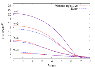
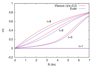
Fig. 1 shows the energy density per unit rapidity (left) and the transverse velocity (right) at various times for both ideal hydrodynamics and for finite viscosity ($\eta/s=0.2$). The effect of viscosity is twofold. The longitudinal pressure is initially reduced and the viscous case does less longitudinal $pdV$ work as in the simple Bjorken expansion Danielewicz:1984ww . This means that at early times the energy per rapidity decreases more slowly in the viscous case. The reduction of longitudinal pressure is accompanied by a larger transverse pressure. This causes the transverse velocity to grow more rapidly. The larger transverse velocity causes the energy density to deplete faster at later times in the viscous case. The net result is that a finite viscosity (even as large as $\eta/s=0.2$) does not integrate to give major deviations from the ideal equations of motion. A preliminary account of this effect was given long ago DT1 .

Figure 1: (Color online) Plot of the energy density per unit rapidity (left) and of the transverse velocity (right) at times of $\tau=1,3,6,9$ fm/c, for $\eta/s=0.2$ (solid red line) and for ideal hydrodynamics (dotted blue line).

We now present results of the 2+1 dimensional boost invariant hydrodynamic model. Fig. 2 shows contour plots of the energy density per unit rapidity in the transverse plane at proper times of $\tau=1,3,6,9$ fm/c. The initial conditions ($\tau=1$) is taken from the Glauber model discussed before.

   

   

Figure 2: (Color online) Contour plot of energy density per unit rapidity in the transverse plane. The contour values working outward are for $\tau=1$ fm/c: 15, 10, 5, 1, 0.1, for $\tau=3$ fm/c: 10, 5, 1, 0.1, for $\tau=6$ fm/c: 3, 2, 1, 0.5 and for $\tau=9$ fm/c: 0.5, 0.375, 0.25, in units of GeV/fm².

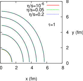
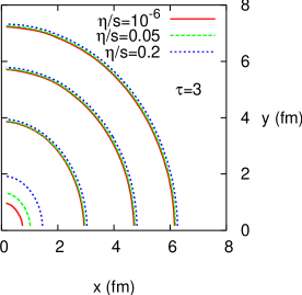
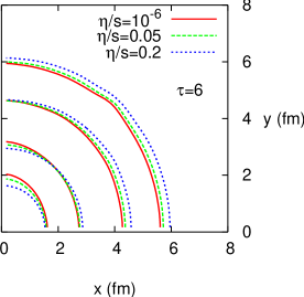
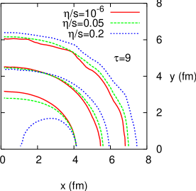
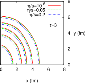
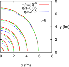
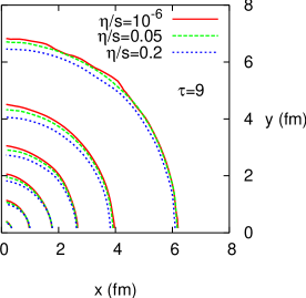
Fig. 3 shows contour plots of the transverse velocity at the same times of $\tau=$1, 3, 6, 9 fm/c. At $\tau=1$ the figure is blank since the velocity in the transverse plane is zero as set by the initial conditions. By looking at the contours of constant $v/c$ one can see that a finite viscosity increases the transverse velocity.

   

   

Figure 3: (Color online) Contour plot of transverse velocity, $v_{\perp}=\sqrt{v_{x}^{2}+v_{y}^{2}}$. The inner most contour is for $v_{\perp}=0.1$ and increases in steps of $\Delta v_{\perp}=0.15$.

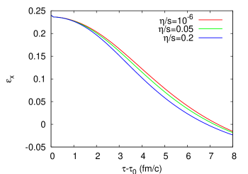
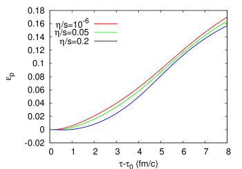
Since we are interested in elliptic flow which originates from the initial spatial anisotropy of the collision region it is useful to see how the spatial and momentum anisotropy develop in time. We therefore look at the following three quantities KSH :

$$\epsilon_{x}=\frac{\langle\langle y^{2}-x^{2}\rangle\rangle}{\langle\langle y^{2}+x^{2}\rangle\rangle}$$

$$\epsilon_{p}=\frac{\langle\langle T^{xx}-T^{yy}\rangle\rangle}{\langle\langle T^{xx}+T^{yy}\rangle\rangle}$$

$$\langle\langle v_{T}\rangle\rangle=\frac{\langle\langle\gamma\sqrt{v_{x}^{2}+v_{y}^{2}}\rangle\rangle}{\langle\langle\gamma\rangle\rangle}$$ (36)

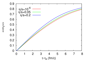
where the double angular bracket $\langle\langle\cdots\rangle\rangle$ denote an energy density weighted average. The spatial ellipticity ($\epsilon_{x}$) is a measure of the spatial anisotropy as a function of time. The spatial anisotropy is what drives the momentum anisotropy ($\epsilon_{p}$). This quantity can be thought of as characterizing the $p_{T}^{2}$ weighted integrated elliptic flow OllitraultSph . The final quantity $\langle\langle v_{T}\rangle\rangle$ is the average radial flow velocity. All three of these quantities are plotted in fig. 4 for $\eta/s$=0.2, 0.05 and $10^{-6}$.

As already shown in the 1+1 dimensional case the finite viscosity case does less longitudinal work. The longitudinal pressure is reduced while the transverse pressure is uniformly increased in the radial direction, i.e. gives no addition $v_{2}$ component. This causes the transverse velocity (as seen in $\langle\langle v_{T}\rangle\rangle$ and fig. 3) to grow more rapidly while $\epsilon_{p}$ lags behind the ideal case. Furthermore, the larger radial symmetric transverse velocity causes a faster decrease in the spatial anisotropy. This further frustrates the build-up of the momentum anisotropy $\epsilon_{p}$. We therefore expect to see a decrease in the integrated $v_{2}$ as the viscosity is increased. This is indeed the case as will be shown. However, this effect is small compared to the change in $v_{2}$ from modifications of the off-equilibrium distribution function.

Figure 4: (Color online) Time evolution of the spatial ellipticity $\epsilon_{x}$, the momentum anisotropy $\epsilon_{p}$, and the energy density weighted transverse flow $\langle\langle v_{\perp}\rangle\rangle$, see Eq. 36.

IV Freezeout

As discussed in the introduction, ideal hydrodynamics is applicable when $\lambda_{mfp}\ll L$ where $L$ denotes the typical system size. When dissipative corrections are included, one must remember that the Navier Stokes equations are derived assuming that the relaxation time $\tau_{R}$ is much smaller than the inverse expansion rate, $\tau_{R}\partial_{\mu}u^{\mu}\ll 1$. Therefore, in the simulations we determine the freezeout surface by monitoring the expansion rate relative to the relaxation time using a generalization of the freezeout criteria first proposed in Bondorf:1978kz ; Heinz:1987ca and later in Hung:1997du .

Specifically, freezeout is signaled when

$$\frac{\eta}{p}\partial_{\mu}u^{\mu}\sim\frac{1}{2}$$ (37)

This combination of parameters can be motivated from the kinetic theory estimates Reif . The pressure is $p\sim\epsilon\left\langle v_{\rm th}^{2}\right\rangle$ with $\left\langle v_{\rm th}^{2}\right\rangle$ the typical quasi-particle velocity and $\epsilon$ the energy density. The viscosity is of order $\eta\sim\epsilon\left\langle v_{\rm th}^{2}\right\rangle\tau_{R}$ with $\tau_{R}$ the relaxation time. Thus the freezeout condition is simply

$$\frac{\eta}{p}\partial_{\mu}u^{\mu}\sim\tau_{R}\partial_{\mu}u^{\mu}\sim\frac{1}{2}$$ (38)

In the model we are considering $\eta/p=\alpha\tau_{2}$ with $\alpha=0.7$ as described in Section II.2.

The value of $\frac{1}{2}$ can be considered as a parameter chosen to be smaller than one. The point is that as the above quantity becomes large the Navier Stokes approximation is no longer applicable and the simulation should freezeout. At this point one would need to include further higher order corrections in the gradients or switch to a kinetic approach.

It is also convenient to have a definition for an analogous freezeout surface in the case of ideal hydrodynamics. One can think of keeping the freezeout surface fixed as $\eta/s$ is taken to zero. Dividing the freezeout criterion by $\eta/s$ and using $s=(\epsilon+p)/T\sim 4p/T$ we define:

$$\chi=\frac{4}{T}\partial_{\mu}u^{\mu}$$ (39)

which involves only quantities in the ideal simulation. This is a separate freezeout parameter independent of the viscosity.

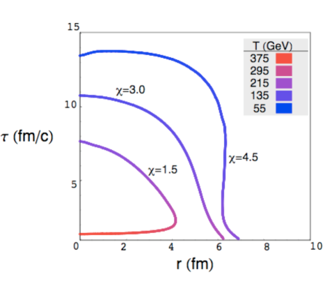
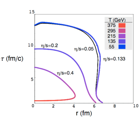
We show in fig. 5 contour plots of the freezeout surface for fixed $\chi$ from both ideal (left plot) and viscous hydrodynamics (right plot). For fixed $\chi$ the freezeout surfaces remain approximately the same in both cases. The freezeout surface from now on will be specified by $\chi$ in order to facilitate a comparison between the ideal and viscous cases when comparing spectra.

We have typically chosen $\chi$ and $\eta/s$ in order that $\frac{\eta}{p}\partial_{\mu}u^{\mu}=0.6$. Thus in Table 1 for $\eta/s=0.2$ we have $\chi=3.0$ and $\frac{\eta}{p}\partial_{\mu}u^{\mu}=0.6$. However, for $\eta/s=0.05$ the freezeout parameter is $\chi=12$ giving an unphysically large surface. This would normally not be the case in a more realistic model with a phase transition present, since in the hadronic phase the viscosity goes like $\eta\sim\frac{T}{\sigma_{0}}$. The change in scaling with temperature would cause the system to freezeout soon after hadronization. We plan on quantifying this statement in a future work. We therefore use $(\eta/p)\partial_{\mu}u^{\mu}=0.225$ when $\eta/s=0.05$ giving $\chi=4.5$. The thin solid curve in the right plot of fig. 5 shows this particular freezeout contour. In table 1 we summarize the freezeout parameters used throughout this work. For a given $\eta/s$ the most physical choice of freezeout parameter $\chi$ is selected such that $(\eta/p)\partial_{\mu}u^{\mu}\approx 0.6$. However, if the viscosity becomes so small that the volume becomes unphysically large (such as for $\eta/s=0.05$) we set $\chi=4.5$ as a maximum. These three physically motivated parameter sets are given in bold in the table.

We should stress that the freezeout surface taken in this work is different from the typical constant temperature surface used in many hydrodynamic simulations. From fig. 5, one can see from the temperature map that the surface is not an isotherm and actually spans a very wide range of temperatures. The freezeout surface is understood by examining the expansion rate in Bjorken geometry

$$\partial_{\mu}u^{\mu}=\partial_{\tau}u^{\tau}+\frac{u^{\tau}}{\tau}+\partial_{x}u^{x}+\partial_{y}u^{y}\,.$$ (40)

The resulting surface is due to a competition between the first two terms in 40 at early times and the last two terms at later times

$\eta/s$	$\frac{\eta}{p}\partial_{\mu}u^{\mu}$	$\chi$
0.05	0.6	12.0
0.05	0.225	4.5
0.05	0.15	3.0
0.2	0.9	4.5
0.2	0.6	3.0
0.133	0.6	4.5

Table 1: Freezeout parameters used throughout this work. For a given $\eta/s$ the most physical choice of freezeout parameter $\chi$ is selected such that $(\eta/p)\partial_{\mu}u^{\mu}\approx 0.6$. However, if the viscosity becomes so small (such as for $\eta/s=0.05$) that the volume becomes unphysically large (see text for discussion) we set $\chi=4.5$ as a maximum. These three physically motivated parameter sets are in bold.

Figure 5: (Color online) Contour plot of various freezeout surfaces for central Au-Au collisions. Left: Surfaces from ideal hydrodynamics where the freezeout condition is set by the parameter $\chi$=1.5, 3 and 4.5. Right: Corresponding viscous solution where $\eta/s$ was fixed by the condition $\frac{\eta}{p}\partial_{\mu}u^{\mu}=0.6$. The thin solid black curve shows the contour set by $\frac{\eta}{p}\partial_{\mu}u^{\mu}=0.225$ for comparison.

V Spectra

V.1 Anisotropy

Before computing the differential spectrum we will compute the momentum anisotropy as a function of time. The momentum anisotropy $A_{2}$ (which differs from $v_{2}$ by the placement of averages) is defined as

$$A_{2}=\frac{\langle p_{x}^{2}\rangle-\langle p_{y}^{2}\rangle}{\langle p_{x}^{2}\rangle+\langle p_{y}^{2}\rangle}=\frac{S_{11}-S_{22}}{S_{11}+S_{22}}\,,$$ (41)

where $S^{ij}$ is the sphericity tensor and can be related to the hydrodynamics fields (i.e. $u^{\mu}$ ,$\pi^{\mu\nu}$, $\Pi$) and moments of the ideal particle distribution function. The explicit form is given in appendix A and generalizes an appendix of Ollitrault OllitraultSph to the viscous case. From a theoretical perspective, $A_{2}$ is preferred because it is almost independent of the details of the particle content of the theory OllitraultSph .

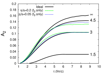
We plot $A_{2}$ in the following manner. At a given proper time we integrate over the surface of constant $\chi$, which has developed by time $\tau$. The remaining part of the surface is fixed by integrating over the matter which has not frozen out ($\chi<\chi_{f.o.}$) at fixed proper time. This can be thought of as a freezeout surface with a flat top at time $\tau$. As time moves forward eventually all of the matter is frozen out over a surface set by constant $\chi$ yielding a constant $A_{2}$.

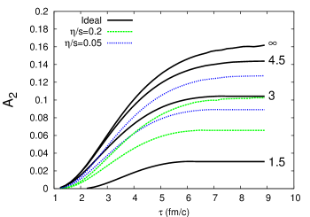
Figure 6 shows $A_{2}$ for four different freezeout surfaces. The figure on the left shows the results using only the ideal contribution to the sphericity (regardless of if viscosity is present). This will be analogous to using only the ideal particle distribution function when generating the spectrum. First look at the solid black curves which are generated using ideal hydrodynamics and a specified $\chi$. For a larger value of $\chi$ a larger space-time region is evolved by hydrodynamics producing a larger elliptic flow or $A_{2}$. The true ideal case where hydrodynamics is universally applicable is given by $\chi=\infty$. We see that for $\chi=4.5$ most of the elliptic flow is reproduced.

In order to assess the role of viscosity we first look at the figure on the left. The dashed curves show $A_{2}$ for $\eta/s=0.05$ and $\eta/s=0.2$ without including viscous corrections to the distribution function. (For clarity, these curves are shown only for $\chi=3.0$ and $\chi=4.5$.) Without the corrections to the distribution function the viscous corrections to $A_{2}$ are modest. The right figure shows the analogous plot, this time including the viscous corrections to the distribution function. The corrections are much larger and we therefore expect the viscosity to decrease the integrated elliptic flow.

Figure 6: (Color online) $A_{2}$ (defined in Eq. 41) as a function of $\tau$. The solid black lines show the ideal result for $\chi=$1.5, 3.0, 4.5 and $\infty$. Also shown in the right and left figures respectively are the viscous results with and without including the viscous correction to the distribution function, for $\chi=3.0$ and $4.5$ and $\eta/s=0.2$ (dashed green curve) and for $\eta/s$=0.05 (dotted blue curve).

V.2 Spectra

The thermal $p_{T}$ and differential $v_{2}$ spectra of particles are generated using the Cooper-Frye formula CF given by

$$E\frac{d^{3}N}{d^{3}p}=\frac{g}{2\pi^{3}}\int_{\sigma}f(p_{\mu}u^{\mu},T)p^{\mu}d\sigma_{\mu}\,.$$ (42)

The thermal distribution function used in the Cooper-Frye formula above also needs to include corrections due to finite viscosity. We therefore write $f=f_{o}+\delta f$ where $f_{o}$ is the ideal particle distribution and $\delta f$ is the viscous correction which has been derived in appendix B and is given by

$$\delta f=\frac{1}{2(e+p)T^{2}}\,f_{o}(1+f_{o})\,p^{\mu}p^{\nu}\left[\pi_{\mu\nu}+\frac{2}{5}\Pi\Delta_{\mu\nu}\right].$$ (43)

For boltzmann statistics $f_{o}(1+f_{o})$ is replaced by $f_{o}$. The elliptic flow is defined as the weighted average of the yields with $\cos(2\phi)$:

$$v2(p_{T})=\langle\cos(2\phi)\rangle_{p_{T}}=\frac{\int_{-\pi}^{\pi}d\phi\cos(2\phi)\frac{dN}{dyp_{T}dp_{T}d\phi}}{\int_{-\pi}^{\pi}d\phi\frac{dN}{dyp_{T}dp_{T}d\phi}}\,,$$ (44)

where $\phi$ is the angle between the decaying particle’s momentum (${\bf p}_{T}$) and the azimuthal angle of the collision region.

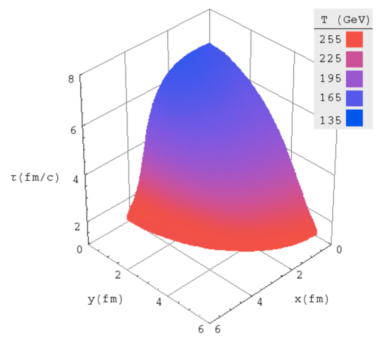
A typical freezeout surface for $\chi=3$ at an impact parameter b=6.5 is shown in fig. 7. Color gradients show the temperature profile on the freezeout surface and as noted before the surface is not necessarily an isotherm.

Figure 7: (Color online) Freezeout surface for semi-central (b=6.5) Au-Au collisions for $\eta/s=0.2$ and $\chi=3.0$.

Differential $p_{T}$ spectra for massless particles are shown in fig. 8 for two different freezeout surfaces: $\chi=3.0$ (left) and $\chi=4.5$ (right). In both plots the ideal case is shown by the solid red line. First we discuss changes to the spectra brought about by modifications to the equations of motion by looking at the spectra generated with the ideal particle distribution ($f_{o}$ only). For both values of viscosity and both freezeout choices a hardening of the spectra is observed. This is expected since viscosity tends to increase the transverse velocity.

The effect from the viscous corrections to the distribution function are more subtle. At earlier times the transverse flow has not fully developed and the longitudinal pressure is reduced while the transverse pressure is increased Teaney:2003kp . This is a consequence of the fact that the shear tensor is traceless. The increase in transverse pressure leads to a hardening of the spectrum after integration over the space-time freezeout surface. This is the case for $\chi=3$ even though the corrections are small. At later times the larger transverse flow alleviates some of the longitudinal shear. When the hydro is finally in a full 3D expansion, the viscous correction tends to reduce the transverse pressure. This changes the sign of the viscous correction term. This is seen for $\chi=4.5$ where the viscous corrections soften the spectrum slightly.

As discussed above, any observable created by using the auxiliary variable $c^{\mu\nu}$ should agree with the results using the physical velocity fields. Therefore we also show the viscous corrections calculated using the physical gradients (denoted by $\delta f_{G}$), i.e., in the local rest frame the $\pi^{ij}$ is approximated by

$$\pi^{ij}=-\eta(\partial^{i}u^{j}+\partial^{j}u^{i}-\frac{2}{3}\delta^{ij}\partial_{l}u^{l})\,,$$ (45)

when computing $\delta f$.

Overall, the corrections to the spectra are small so it is hard to see any differences between the two calculations. This will not be the case for the differential elliptic flow where this comparison will be more important.

Figure 8: (Color online) Differential transverse momentum spectra for Au-Au collisions at b=6.5 fm. The left plot is for freeze-out parameter $\chi=3$ and the right for $\chi=4.5$. In both plots the ideal case is shown by the solid red curve. Then the viscous case is shown without including the viscous corrections to the distribution function and is denoted by $f_{o}$. The addition of the viscous correction to the distribution function is generated in two different ways. $\delta f_{\pi}$ is calculated using the auxiliary tensor $c^{\mu\nu}$ while $\delta f_{G}$ is calculated using the physical gradients i.e., $\pi^{\mu\nu}=-\eta\langle\partial^{\mu}\partial^{\nu}\rangle$.

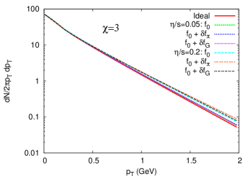
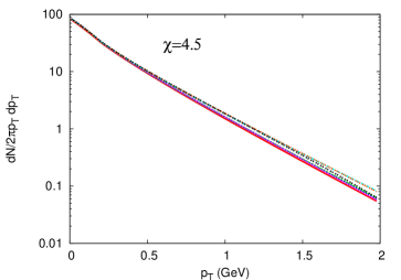
Figure 9 shows the differential elliptic flow using the same parameter set from the $p_{T}$ spectrum. The solid red curves shows the ideal spectrum and, as expected, a larger elliptic flow is generated for $\chi=4.5$ compared to $\chi=3$ since a larger fraction of the space-time volume is described by hydrodynamics.

The viscous correction to the equations of motion causes only a small change in the elliptic flow as seen by comparing the results at finite viscosity using $f_{o}$ only with the ideal case. For $\chi=3$ the change is almost negligible. For $\chi=4.5$ deviations are on the order of 2% at $p_{T}=2$ GeV.

Figure 9: (Color online) Differential $v_{2}$ spectra for Au-Au collisions at b=6.5 fm. The resulting curves are generated in the same way as described for the $p_{T}$ spectra in fig. 8

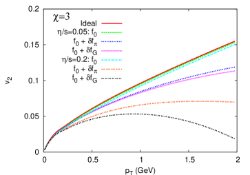
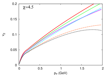
Including the viscous corrections to the distribution function can bring about large changes in the elliptic flow. We show the corrections due to the auxiliary variable by $\delta f_{\pi}$ and those from the gradients by $\delta f_{G}$ and we expect the two results to agree. When the two results start to diverge the gradient expansion is no longer valid and a kinetic description is really required.

Based on our discussion in section IV the viscosity is what sets the freezeout surface. For $\eta/s=0.2$ we find that $\chi=3$ (figure on left). In this case the viscous corrections are large but can only be trusted up to $p_{T}\approx 1$ GeV. We also show for comparison the spectra for $\eta/s=0.05$ which can be trusted past 2 GeV. For $\eta/s=0.05$ we take $\chi=4.5$ for reasons discussed in section IV. Again, the viscous correction decreases the elliptic flow as a function of $p_{T}$. Also shown are the spectra for $\eta/s=0.2$ and the corrections are larger. In both cases the spectra can be trusted past $p_{T}$ = 2 GeV.

VI Discussion and comparison with other works

VI.1 Discussion

In summary we now make several conclusions regarding the effects of shear viscosity on heavy ion collisions.

We first recall the setup. The paper is restricted to an ideal gas equation of state $p=\frac{1}{3}\epsilon$ and sets the initial non-equilibrium fields to the value expected from the navier stokes equations $\pi^{ij}=-\eta\left\langle\partial^{i}u^{j}\right\rangle$. The initial distribution of entropy density follows the distribution of participants. (This could be changed to a Color Glass Condensate model initial conditions Hirano:2005xf .) The paper simulates a fluid model based on Ottinger which is similar but differs from that of Israel and Stewart. However all models should ultimately agree on the magnitude of viscous corrections provided the viscosity is sufficiently small.

Several technical notes warrant discussion here. An algorithm for a reliable solution of the viscous model was developed by Pareschi Pareschi and is presented in appendix D which achieves uniform numerical accuracy across a wide range of relaxation times. For small enough relaxation times the auxiliary fields $\pi^{ij}$ should relax to the form expected from the Navier-Stokes equation $\pi^{ij}\simeq-\eta\left\langle\partial^{i}u^{j}\right\rangle$. To see this good/reasonable convergence for small/modest viscosities see appendix D.2. Generically, relaxation models for viscosity have long time parameters (the shear viscosity $\eta$ in this case) and short time parameters. In the model considered here, $\alpha$ (see appendix C) is the short time parameter while in the Israel-Stewart theory this short time parameter is $\eta/[(\epsilon+p)\tau_{\pi}]$. These short time parameters can be constrained by the $f$-sum rule KadanoffMartin ; Teaney_corr ; PTcorr and is discussed further in appendix C. In general the results should not depend on these short time parameters.

We now summarize our physical results. The integrated viscous corrections to the flow are small. This was seen in both the hydrodynamic fields and also in the differential and integrated elliptic flow when the thermal distribution function was restricted to the ideal form. (The remainder of this paragraph discusses only results with this restriction.) For the integrated $v_{2}$ this is seen in the left plot of fig. 6 where $A_{2}$ is shown for ideal runs and viscous runs at $\eta/s=0.05$ and $0.2$. Corrections due to the modified flow pattern are also small in the differential $v_{2}$ spectrum as seen in fig. 9 by comparing the ideal and viscous runs (again with $f_{o}$ only.) Although there is the possibility for the elliptic flow to be modified from variations in the freezeout surface across different runs this was minimized by freezing out on contours of constant $\chi$. One can see from fig. 5 that the space-time freezeout contours are about the same at zero and finite viscosity. The fact that only small changes in the fields are seen when including viscosity is not surprising. The time scale of any heavy ion collision is much shorter then the time needed for dissipative effects to integrate and become large.

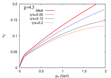
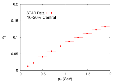
Even though viscosity does not modify the flow strongly we have shown that there are still large corrections to the particle spectra due to off-equilibrium corrections to the ideal particle distribution function. Any bounds for the viscosity (at least from this paper) would have to come from the $v_{2}$ spectra. As Lindblom Lindblom and earlier work by others KadanoffMartin has clarified, any observable computed from the auxiliary fields $\pi^{ij}$ must agree with the same observable generated by the physical gradients $-\eta\left\langle\partial^{i}u^{j}\right\rangle$. When deviations are seen the viscous corrections can no longer be trusted. For a freezeout surface set by $\chi=4.5$ the viscous corrections agree with gradients up to 2 GeV for viscosities as large as $\eta/s=0.2$ as seen in figure 9. It is therefore safe to use only the auxiliary variable when generating spectra for this particular parameter set. In figure 10 we show a summary plot of the differential elliptic flow. We now show one additional curve for $\eta/s=0.133$ yielding $(\eta/p)\partial_{\mu}u^{\mu}=0.6$ for this particular choice of freezeout surface. We believe that this choice of parameters is the closest physical scenario. The right plot of figure 10 shows the measured elliptic flow as measured by the STAR collaboration Adams:2004bi . We do not intend to make a comparison, but simply would like to keep the data in mind. Nevertheless since this simulation was performed with a massless gas which has the largest elliptic flow, it seems difficult to imagine that the $\eta/s\mbox{~{}{\raisebox{1.72218pt}{$>$}} {\raisebox{-2.58334pt}{$\sim$}}~{}}0.35$ will ever fit the data even if the initial conditions are modified along the lines of Ref. Hirano:2005xf .

Before a realistic comparison with data can be made the QGP/hadronic phase transition must be taken into account. In the vicinity of the phase transition it is possible that the shear viscosity may become very large. Also, a more realistic model for the hadronic gas would be the hard sphere model where $\eta\sim\frac{T}{\sigma_{0}}$. This would adjust at what point the simulation freezes out and would therefore effect spectrum. There is most likely a finite bulk viscosity due to the fluctuations of the QGP and hadron concentrations in the mixed phase or from chemical off-equilibrium in the hadronic phase Kharzeev:2007wb . A final issue that should be taken into consideration is that particles of different mass could possibly freezeout on different surfaces. These issues will be addressed in a future work.

Figure 10: Left: Summary plot showing $v_{2}$ for massless particles for simulations using ideal hydro and $\eta/s=0.05,0.2$. Right: Charged hadron $v_{2}$ data using the standard reaction plane method as measured in Au-Au collisions at $\sqrt{s}=200$ GeV for a centrality selection of 10% to 20% Adams:2004bi .

VI.2 Comparison

We now compare our results to some other groups, first with the recent results of Song and Heinz Heinzv2 where they computed differential $v_{2}$ spectrum in Cu-Cu collisions.

One conclusion they found is that varying the initial conditions do not change the end result, even in the extreme condition when the equilibrium stress tensor is set to zero $\pi^{\mu\nu}(\tau_{0})=0$. This insensitivity is similar to the insensitivity to the short time parameter $\alpha$ indicated in appendix C.1.

Song and Heinz also found that the viscosity substantially changes the flow. Their differential $v_{2}$ spectra changes dramatically when viscosity is included, even if the particles freezeout using an ideal distribution. In our case there is almost no change in $v_{2}$ when viscosity is present when freezing out with $f_{o}$ only, while in their case they see $v_{2}$ decrease by a factor of two at 3 GeV due to changes in the flow alone (see their fig. 4). It is possible that this difference is due to their inclusion of a phase transition in their equation of state. Once the plasma phase reaches the phase transition the momentum anisotropy ($\epsilon_{p}$) stalls in their model staying constant for the entire mixed phase (and only growing slightly in the hadronic phase). Therefore after freezing out the elliptic flow is in some sense probing earlier times where viscous corrections to the flow may be larger. Actually, if one looks at our $\epsilon_{p}$ in figure 4 the largest differences between the ideal and viscous cases is for earlier times. This explanation should be verified.

When the viscous corrections to the distribution function are added we both see qualitatively the same behavior. The viscous correction gets larger with transverse momentum eventually driving the elliptic flow below zero. It is impossible to make quantitative comparisons until we include a phase transition and run simulations with smaller systems sizes, which we plan on doing in a future work.

We now compare our work with that of Baier and Romatschke Baier:2006gy ; Romatschke:2007jx for the flow and $p_{T}$ spectrum in central collisions. They also find that the viscosity does not integrate to significantly modify the ideal flow. We both find qualitatively the same behavior confirming even earlier works Muronga ; DT1 . Finite viscosity causes the temperature to drop slowly at earlier times and more quickly at later times compared to the ideal case. This effect was already discussed in section III

Although the freeze-out conditions in this work differ from those of Baier and Romatschke, we find qualitatively the same behavior when comparing $p_{T}$ spectra, i.e. a hardening of spectra at large $p_{T}$.

In comparison with the differential $v_{2}$ results by Romatschke and Romatschke RRv2 we see qualitatively the same behavior. In this case the comparison is more direct since both simulations were performed using Au-Au collisions at the same $\sqrt{s}$. Comparing our results for $\chi=4.5$, we see that our $v_{2}$ drops by $\approx$50% at $p_{T}=2$ GeV. This is on the same order as seen in fig. 3 of Ref. RRv2 . However they do not show contributions from flow and the distribution function separately so it is hard to make any definitive comparisons.

VII Conclusions

In this work we have outlined the equations of motion necessary for a casual description of viscous relativistic hydrodynamics and have shown results using initial conditions tuned to Au-Au collisions at $\sqrt{s}\approx 200$ GeV. The results indicate that the viscous correction to the ideal equations of motion are small. The goal of this work was to calculate the viscous correction to differential $v_{2}$ spectra. Even though modifications to $v_{2}$ from the flow are small the effect of the off-equilibrium distribution function can bring about large changes in $v_{2}(p_{T})$. By requiring observables calculated with the auxiliary fields to agree with those calculated with the physical gradients one can identify where a hydrodynamic description is reliable.

Appendix A Sphericity

In this appendix we show (following OllitraultSph ) how the momentum anisotropy, expressed through $A_{2}$, can be related to hydrodynamic quantities. As discussed in the text $A_{2}$ is defined as

$$A_{2}=\frac{S_{11}-S_{22}}{S_{11}+S_{22}}=\frac{\langle p_{x}^{2}\rangle-\langle p_{y}^{2}\rangle}{\langle p_{x}^{2}\rangle+\langle p_{y}^{2}\rangle}.$$ (46)

The sphericity tensor $S_{ij}$ is calculated from the third moment of the momentum distribution function

$$S_{ij}=\int_{\sigma}d\sigma_{\mu}S^{\mu\nu\rho},$$ (47)

where $d\sigma_{\mu}$ is a differential element of the freezeout surface and the third-rank tensor, $S^{\mu\nu\rho}$ is defined as

$$S^{\mu\nu\rho}=\int p^{\mu}p^{\nu}p^{\rho}f(p)\frac{d^{3}p}{(2\pi)^{3}E_{\bf p}}.$$ (48)

In order to relate the sphericity tensor to hydrodynamic quantities we follow the same steps as was done in OllitraultSph but also include the additional terms coming from viscous corrections. First one substitutes the expression for the momentum distribution function with the appropriate viscous correction term into the above equation for the third-rank sphericity tensor

$$S^{\mu\nu\rho}=S_{I}^{\mu\nu\rho}+S_{V}^{\mu\nu\rho}.$$ (49)

The subscripts $I$ and $V$ correspond to the ideal and viscous contributions respectively and are defined as

$$S_{I}^{\mu\nu\rho}=\int p^{\mu}p^{\nu}p^{\rho}f_{o}(p)\frac{d^{3}p}{(2\pi)^{3}E_{\bf p}},$$ (50)

$$S_{V}^{\mu\nu\rho}=\frac{1}{2sT^{3}}\left[\pi_{\alpha\beta}+\frac{2}{5}\Pi\Delta_{\alpha\beta}\right]S_{5}^{\mu\nu\rho\alpha\beta},$$ (51)

where we have defined the fifth-rank tensor

$$S_{5}^{\mu\nu\rho\alpha\beta}=\int p^{\mu}p^{\nu}p^{\rho}p^{\alpha}p^{\beta}f_{o}(p)\frac{d^{3}p}{(2\pi)^{3}E_{\bf p}}.$$ (52)

Lorentz invariance sets the form of both $S_{I}$ and $S_{5}$ as follows

$$S_{I}^{\mu\nu\rho}=Au^{\mu}u^{\nu}u^{\rho}+B(g^{\mu\nu}u^{\rho}+\text{permutations})$$ (53)

$$,S_{5}^{\mu\nu\rho\alpha\beta}=Cu^{\mu}u^{\nu}u^{\rho}u^{\alpha}u^{\beta}+D(u^{\mu}u^{\nu}u^{\rho}g^{\alpha\beta}+\text{permutations})+$$

$$E(u^{\mu}g^{\nu\rho}g^{\alpha\beta}+\text{permutations}).$$ (54)

The coefficients A..E can be found in the same manner as was done previously in OllitraultSph . Quoting the result:

$$A=n(2\langle\!\langle E^{2}\rangle\!\rangle-m^{2})$$ (55)

$$B=n\frac{\langle\!\langle E^{2}\rangle\!\rangle-m^{2}}{3}$$ (56)

$$C=n(16\langle\!\langle E^{4}\rangle\!\rangle-16m^{2}\langle\!\langle E^{2}\rangle\!\rangle+3m^{4})/3$$ (57)

$$D=-n(8\langle\!\langle E^{4}\rangle\!\rangle-11m^{2}\langle\!\langle E^{2}\rangle\!\rangle+3m^{4})/15$$ (58)

$$E=n(\langle\!\langle E^{4}\rangle\!\rangle-2m^{2}\langle\!\langle E^{2}\rangle\!\rangle+m^{4})/15$$ (59)

The results for $S^{11}_{I}$ and $S^{22}_{I}$ can be expressed in terms of hydrodynamic quantities:

$$S^{11}_{I}=\int_{\sigma}(Au_{x}^{2}+B)u^{\mu}d\sigma_{\mu}+2B\int_{\sigma}u^{x}d\sigma_{x}$$

$$S^{22}_{I}=\int_{\sigma}(Au_{y}^{2}+B)u^{\mu}d\sigma_{\mu}+2B\int_{\sigma}u^{y}d\sigma_{y}$$ (60)

The result for $S^{11}_{V}$ and $S^{22}_{V}$ can be found making use of the following three identities:

$$u^{\alpha}\pi_{\alpha\beta}=0$$

$$g^{\alpha\beta}\pi_{\alpha\beta}=0$$

$$u^{\alpha}\Delta_{\alpha\beta}=0$$ (61)

Therefore, the viscous correction to the sphericity tensor is given as

$$S^{11}_{V}=\frac{1}{2sT^{3}}\int_{\sigma}2E\left[\pi^{xx}u^{\mu}d\sigma_{\mu}+2u^{x}\pi^{x\mu}d\sigma_{\mu}\right]+$$

$$\frac{\Pi}{5sT^{3}}\int_{\sigma}\left[3Du_{x}^{2}u^{\mu}d\sigma_{\mu}+E\left(5u^{\mu}d\sigma_{\mu}+10u^{x}d\sigma_{x}-6u_{x}^{2}u^{\mu}d\sigma_{\mu}\right)\right],$$ (62)

and

$$S^{22}_{V}=\frac{1}{2sT^{3}}\int_{\sigma}2E\left[\pi^{yy}u^{\mu}d\sigma_{\mu}+2u^{y}\pi^{y\mu}d\sigma_{\mu}\right]+$$

$$\frac{\Pi}{5sT^{3}}\int_{\sigma}\left[3Du_{y}^{2}u^{\mu}d\sigma_{\mu}+E\left(5u^{\mu}d\sigma_{\mu}+10u^{y}d\sigma_{y}-6u_{y}^{2}u^{\mu}d\sigma_{\mu}\right)\right].$$ (63)

Appendix B Viscous correction to the distribution function

The thermal $p_{T}$ and differential $v_{2}$ spectra of particles are generated using the Cooper-Frye formula CF

$$E\frac{d^{3}N}{d^{3}p}=\frac{g}{2\pi^{3}}\int_{\sigma}f(p_{\mu}u^{\mu},T)p^{\mu}d\sigma_{\mu},$$ (64)

where $d\sigma_{\mu}$ is the normal vector to the freezeout surface set by the condition of constant $\chi$. For the geometry we are considering here we have

$$p_{\mu}u^{\mu}=m_{T}u^{0}\cosh(\eta_{s})-p_{1}u^{1}-p_{2}u^{2},$$ (65)

$$p^{\mu}d\sigma_{\mu}=\tau(m_{T}\cosh(\eta_{s})d\sigma_{0}+p^{1}d\sigma_{1}+p^{2}d\sigma_{2}).$$ (66)

Following Teaney:2003kp ; AMY we will make a second moment ansatz for the thermal distribution function. We first write the stress tensor as

$$T^{\mu\nu}=\epsilon u^{\mu}u^{\nu}+(p+\Pi)\Delta^{\mu\nu}+\pi^{\mu\nu},$$ (67)

where $\pi^{\mu\nu}$ is symmetric traceless and satisfies $\pi^{\mu\nu}u_{\nu}=0$. Then we subsequently make an ansatz for the thermal distribution $f\rightarrow f_{o}+\delta f$

$$\delta f=\frac{1}{(e+p)T^{2}}\,f_{o}(1+f_{o})\,p^{\mu}p^{\nu}\left[\frac{C_{1}}{2}\pi_{\mu\nu}+\frac{C_{2}}{5}\Pi\Delta_{\mu\nu}\right]$$ (68)

where $C$ is a constant and the factor $1/\left[(e+p)T^{2}\right]$ has been inserted for later convenience. To determine the constant $C$ we demand that

$$T^{\mu\nu}=\int\frac{d^{3}p}{(2\pi)^{3}}\,\frac{p^{\mu}p^{\nu}}{E_{{\bf p}}}\,f.$$ (69)

Working in the local rest frame this becomes a condition that

$$\Pi\delta^{ij}+\pi^{ij}=\left\{\frac{1}{(e+p)T^{2}}\,\int\frac{d^{3}p}{(2\pi)^{3}}\,\frac{p^{i}p^{j}p^{l}p^{m}}{E_{\bf p}}\,f_{o}(1+f_{o})\,\right\}\left[\frac{C_{1}}{2}\pi_{lm}+\frac{C_{2}}{5}\Pi\delta_{lm}\right].$$ (70)

The integral over the three momentum in curly braces can be expressed as

$$I\left(\delta^{ij}\delta^{lm}+\delta^{il}\delta^{jm}+\delta^{im}\delta^{jl}\right),$$ (71)

where

$$I=\frac{1}{15(e+p)T^{2}}\int\frac{d^{3}p}{(2\pi)^{3}}\,\frac{\left|{\bf p}\right|^{4}}{E_{\bf p}}\,f_{o}(1+f_{o}).$$ (72)

Inserting Eq. (71) into Eq. (70) we see that

$$C_{1}=C_{2}=\frac{1}{I}.$$ (73)

We record two limiting cases of this integral. In the massless limit with zero chemical potential the integral is easily performed and yields

$$I = \frac{90\zeta(5)}{\pi^{4}}\approx 0.958.$$ (74)

In the classical limit the factor $f_{o}(1+f_{o})$ is replaced by

$$f_{o}(1+f_{o})\rightarrow f_{o}=e^{{-(E_{\bf p}-\mu)}/T},$$ (75)

and the integral is easily performed using the integral representation of the modified Bessel functions

$$I = \frac{1}{(e+p)T^{2}}\,\left[\frac{m^{3}T^{3}}{2\pi^{2}}\,e^{\mu/T}K_{3}(m/T)\right]=1.$$ (76)

Appendix C Relaxation Time

It was shown in Teaney_corr ; PTcorr that for a weakly interacting theory the transport time scale $\tau_{R}$ is much longer than the inverse temperature. This separation of time scales is seen in the spectral density which will have a sharp peak at small frequencies $\omega\sim 1/\tau_{R}\ll T$. In Teaney_corr ; PTcorr a sum rule for this peak was derived relating the small time ($t\ll\tau_{R}$) behavior of hydrodynamic correlators to the microscopic time scale. The statement of this sum rule can be written as:

$$\frac{T}{k^{2}}\partial_{t}\chi_{gg}^{L}({\bf k},t)|_{t\sim 1/\Lambda}\approx T(\epsilon+p)\langle\frac{3}{5}v_{{\bf p}}^{2}\rangle$$

$$\frac{T}{k^{2}}\partial_{t}\chi_{gg}^{T}({\bf k},t)|_{t\sim 1/\Lambda}\approx T(\epsilon+p)\langle\frac{v_{{\bf p}}^{2}}{5}\rangle$$

(77)

where $v_{{\bf p}}$ is ${\bf p}/E$ and $\Lambda$ is a cut-off such that $1/\tau_{R}\ll\Lambda\ll T$. $\chi_{gg}$ is the retarded correlator of $T^{0i}$ and can be found in the framework of linear response theory. A small velocity field is turned on with a perturbing Hamiltonian

$$H=H_{0}-\int d^{3}{\bf x}v^{i}({\bf x},t)T^{0i}({\bf x},t),$$ (78)

and suddenly switched off at t=0: $v^{i}({\bf x},t)=e^{\epsilon t}\theta(-t)v_{0}^{i}({\bf x})$. In the framework of linear response this yields

$$\partial_{t}\langle T^{0i}({\bf k},t)\rangle=-\chi_{gg}^{ij}({\bf k},t)v_{0}^{i}({\bf k}).$$ (79)

The stress tensor can be expressed as the equilibrium stress tensor plus small corrections:

$$\langle T^{00}\rangle=e+\epsilon({\bf x},t)$$ (80)

$$\langle T^{0i}\rangle=0+g^{i}({\bf x},t),$$ (81)

where ${\bf g}\equiv{\bf v}(e+p)$. The linearized hydrodynamic equations are:

$$\partial_{t}\epsilon+\partial_{i}g^{i}=0$$ (83)

$$\partial_{t}g^{j}+\partial_{i}\tau^{ij}=0,$$ (84)

where

$$\tau^{ij}=\delta^{ij}p-\eta(\partial^{i}u^{j}+\partial^{j}u^{i}-\frac{2}{3}\delta^{ij}\partial_{l}u^{l})-\delta^{ij}\zeta\partial_{l}u^{l},$$ (85)

in the Navier-Stokes limit. However, since we are interested in relating the short time parameters of the theory used in this work to microscopic quantities we take $\tau^{ij}$ from the second-order equations

$$\tau^{ij}=p(\delta^{ij}-\alpha c^{ij}).$$ (86)

We now have all the pieces needed in order to evaluate the left hand side of eq. 77. First, for small $c$ the evolution equation simplifies to

$$\partial_{t}c^{ij}-(\partial^{i}u^{j}+\partial^{j}u^{i})=\frac{1}{\tau_{0}}c^{l}_{l}\delta^{ij}+\frac{1}{\tau_{2}}(c^{ij}-\frac{1}{3}c^{l}_{l}\delta^{ij}).$$ (87)

We can now differentiate eqn. 84 with respect to time, substitute in the evolution equation and immediately take the $t\to 0$ limit in order to obtain

$$\partial_{t}^{2}g^{j}|_{t=0}=-c_{s}^{2}\partial_{j}\partial_{t}\epsilon-\alpha p\partial_{i}[\partial^{i}u^{j}+\partial^{j}u^{i}].$$ (88)

We now make use of the first linearized hydrodynamic equation, $\partial_{t}\epsilon=-(\epsilon+p)\partial_{i}v^{i}$, which can be substituted into eq. 88. After taking a spatial Fourier transform we get:

$$\partial_{t}^{2}g^{j}|_{t=0}=-c_{s}^{2}(\epsilon+p)k_{j}k_{i}v^{i}-p\alpha[k^{2}v^{j}+k^{i}k^{j}v^{i}].$$ (89)

This equation can be decomposed into its transverse and longitudinal pieces by defining $g^{j}=g^{jT}+\frac{k^{j}}{k}g^{L}$ where $k^{j}g^{jT}=0$. Since we are only interested in the shear viscosity we can simply look at the transverse component

$$\partial_{t}^{2}g^{jT}=-p\alpha k^{2}v^{j},$$ (90)

and when substituted into the sum rule, eqn. 77, we obtain the result

$$\alpha=\frac{4}{5}.$$ (91)

A similar analysis can be done for the Israel-Stewart equations IS as well:

$$\tau^{ij}=p\delta^{ij}+\pi^{ij}$$ (92)

$$\partial_{t}\pi^{ij}=\frac{1}{\tau_{\pi}}[-\eta\langle\partial^{i}v^{j}\rangle-\pi^{ij}]$$ (93)

with the result

$$\tau_{\pi}=\frac{5\eta}{4p}.$$ (94)

C.1 Dependence on small time parameter

It was discussed throughout the paper that the results should not depend on the small time parameter. In order to test this we have generated $v_{2}$ spectrum with a value of $\alpha=0.35$ compared to the default value of $\alpha=0.7$ used throughout this work. This is shown in Fig. 11 for $\eta/s=0.5$ (left) and $\eta/s=0.2$ (right) for a fixed freeze-out surface parameter $\chi=3$. The ideal curves are also shown for reference.

Figure 11: Differential $v_{2}$ spectrum for Au-Au collisions at b=6.5 fm. Left: $\eta/s=0.05$ Right: $\eta/s=0.2$ Each figure shows spectrum calculated with the default small time parameter $\alpha=0.7$ and half of this value, $\alpha=0.35$.

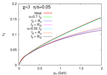
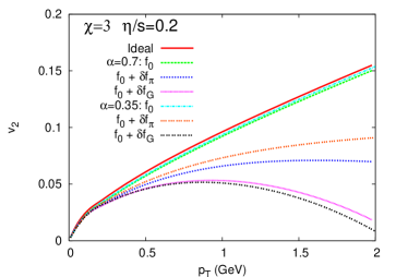
The deviations between the results using two different values of $\alpha$ are small. The flow is hardly changed as seen by comparing the spectrum generated using only the ideal distribution function, $f_{o}$. In this case, for both values of $\eta/s$, the results differ by less than 1%. When including the viscous correction to the spectrum the results still agree reasonably well.

Appendix D Algorithm

In this appendix the algorithm used in order to solve Eqn’s 20-26 is outlined. The numerical evaluation of the above system of hyperbolic equations is difficult because one would like would like to achieve uniform numerical accuracy across a range of relaxation times. In order to achieve this we use a discretization method first proposed by Pareschi Pareschi which can numerically solve the above equations in both the stiff and unstiff regions.

We use notation such that the term $x^{n}_{i,j}$ refers to the value of x at discrete time $t^{n}$ and grid point $(x,y)=(x_{i},y_{j})$ with i and j always referring to the x and y grid coordinates. Any variable absent of an index represents a continuous variable not yet specified at a given point. At times we use a simplified notation for the discretized fields such that $u(x_{i},y_{j},t^{n})=u^{n}_{i,j}$.

For completeness we outline the integration routine developed by Pareschi . Our goal is to solve equations of the form

$$u_{t}(x,y,t)+f_{x}(u)+h_{y}(u)=g(u),$$ (95)

where u, f, h, and g are arbitrary functions. We use the standard notation that for a finite volume element the value of a field at the point $(x_{i+\frac{1}{2}},y_{j+\frac{1}{2}})$ and at a time $t=t^{n}$ is given by:

$$u^{n}_{i+\frac{1}{2},j+\frac{1}{2}}=\frac{1}{\Delta x\Delta y}\int^{x_{i+1}}_{x_{i}}\int^{y_{j+1}}_{y_{j}}u(x,y,t^{n})dxdy$$ (96)

We then integrate eq. 95 over the region $[x_{i},x_{i+1}]\times[y_{j},y_{j+1}]\times[t^{n},t^{n+1}]$ yielding:

$$u^{n+1}_{i+\frac{1}{2},j+\frac{1}{2}}=\frac{1}{\Delta x\Delta y}\Bigglb[\int^{x_{i+1}}_{x_{i}}\int^{y_{j+1}}_{y_{j}}u(x,y,t^{n})dxdy+\int^{y_{j+1}}_{y_{j}}\int^{t^{n+1}}_{t^{n}}\biglb(f(x_{i+1},y,t)-f(x_{i},y,t)\bigrb)dydt+$$

$$+\int^{x_{i+1}}_{x_{i}}\int^{t^{n+1}}_{t^{n}}\biglb(h(x,y_{j+1},t)-h(x,y_{j},t)\bigrb)dxdt+\int^{x_{i+1}}_{x_{i}}\int^{y_{j+1}}_{y_{j}}\int^{t^{n+1}}_{t^{n}}g(x,y,t)dxdydt\Biggrb]$$

(97)

The first integral over the field $u$ in the above equation (97) can be discretized by constructing a piecewise linear approximation of u(x,y,t) over the integration region:

$$\int^{y_{j+1}}_{y_{j}}u(x,y,t^{n})dy=\int^{y_{j+\frac{1}{2}}}_{y_{j}}\left[u(x,y_{j},t^{n})+(y-y_{j})u_{y}(x,y_{j},t^{n})\right]dy+$$

$$+\int^{y_{j+1}}_{y_{j+\frac{1}{2}}}\left[u(x,y_{j+1},t^{n})+(y-y_{j+1})u_{y}(x,y_{j+1},t^{n})\right]dy$$ (98)

Using the corresponding linear approximation for the integration over $[x,x_{i+1}]$ and performing the elementary integration over $x$ and $y$ the following discretization is found:

$$\frac{1}{\Delta x\Delta y}\int^{x_{i+1}}_{x_{i}}\int^{y_{j+1}}_{y_{j}}u(x,y,t^{n})dxdy=\frac{1}{4}\biglb(u^{n}_{i,j}+u^{n}_{i+1,j}+u^{n}_{i,j+1}+u^{n}_{i+1,j+1}\bigrb)+$$

$$+\frac{\Delta x}{16}\partial_{x}\biglb(u^{n}_{i,j}-u^{n}_{i+1,j}+u^{n}_{i,j+1}-u^{n}_{i+1,j+1}\bigrb)+\frac{\Delta y}{16}\partial_{y}\biglb(u^{n}_{i,j}+u^{n}_{i+1,j}-u^{n}_{i,j+1}-u^{n}_{i+1,j+1}\bigrb)$$ (99)

For the time integrals over the fluxes (second and third term in eq. 97) a general trapezoidal rule is used:

$$\frac{1}{\Delta t}\int^{t^{n+1}}_{t^{n}}f(x,y,t)dt\approx\mu f(x,y,t^{n+\alpha})+\nu f(x,y,t^{n})$$ (100)

where $f^{n+\alpha}$ will be given explicitly by a predictor step to be defined later. The time integrals over the source term (last term in eq. 97 will also be given by a general trapezoidal rule which will result in an implicit equation between the sources and charges.

$$\frac{1}{\Delta t}\int^{t^{n+1}}_{t^{n}}g(x,y,t)dt\approx\zeta g(x,y,t^{n+1})+\eta g(x,y,t^{n})$$ (101)

In order to ensure second order accuracy in space the second and third integrals over the fluxes in eq. 97 are evaluated after the time integrations using the standard midpoint rule and trapezoidal rule depending on the time:

$$\text{for }t=t^{n+1}:\text{ }\frac{1}{\Delta x}\int^{x_{i+1}}_{x_{i}}h(x,y,t)dx\approx h(x_{i+\frac{1}{2}},y,t)$$ (102)

$$\text{for }t\in[t^{n},t^{n+1}]:\text{ }\frac{1}{\Delta x}\int^{x_{i+1}}_{x_{i}}h(x,y,t)dx\approx\frac{1}{2}\biglb[h(x_{i+1},y,t)+h(x_{i},y,t)\bigrb]$$ (103)

After evaluating all the integrals in eq. 97 using the above rules for discretization the final result for $u_{i+\frac{1}{2},j+\frac{1}{2}}^{n+1}$ is:

$$u_{i+\frac{1}{2},j+\frac{1}{2}}^{n+1}=\frac{1}{4}\biglb(u^{n}_{i,j}+u^{n}_{i+1,j}+u^{n}_{i,j+1}+u^{n}_{i+1,j+1}\bigrb)+$$

$$+\frac{\Delta x}{16}\partial_{x}\biglb(u^{n}_{i,j}-u^{n}_{i+1,j}+u^{n}_{i,j+1}-u^{n}_{i+1,j+1}\bigrb)+\frac{\Delta y}{16}\partial_{y}\biglb(u^{n}_{i,j}+u^{n}_{i+1,j}-u^{n}_{i,j+1}-u^{n}_{i+1,j+1}\bigrb)+$$

$$+\frac{\Delta t}{2\Delta x}\Biglb[\mu\Biglb(f_{i,j}^{n}+f_{i,j+1}^{n}-f_{i+1,j}^{n}-f_{i+1,j+1}^{n}\Bigrb)+\nu\Biglb(f_{i,j}^{n+\alpha}+f_{i,j+1}^{n+\alpha}-f_{i+1,j}^{n+\alpha}-f_{i+1,j+1}^{n+\alpha}\Bigrb)\Bigrb]+$$

$$+\frac{\Delta t}{2\Delta y}\Biglb[\mu\Biglb(h_{i,j}^{n}+h_{i+1,j}^{n}-h_{i,j+1}^{n}-h_{i+1,j+1}^{n}\Bigrb)+\nu\Biglb(h_{i,j}^{n+\alpha}+h_{i+1,j}^{n+\alpha}-h_{i,j+1}^{n+\alpha}-h_{i+1,j+1}^{n+\alpha}\Bigrb)\Bigrb]+$$

$$+\Delta t\biglb[\frac{\xi}{4}\biglb(g_{i,j}^{n+\alpha}+g_{i+1,j}^{n+\alpha}+g_{i,j+1}^{n+\alpha}+g_{i+1,j+1}^{n+\alpha}\bigrb)+\eta g_{i+\frac{1}{2},j+\frac{1}{2}}^{n+1}\bigrb]$$

(104)

The terms at time $t^{n+\alpha}$ are taken from the solution of the predictor step:

$$u_{i,j}^{n+\alpha}=u_{i,j}^{n}-\Delta t\alpha\biglb(\partial_{x}f_{i,j}^{n}+\partial_{y}h_{i,j}^{n}-g_{i,j}^{n+\alpha}\bigrb)$$ (105)

As shown in Pareschi , second order accuracy conditions give the weights used in the discretization as a function of $\alpha$. We choose $\alpha=1/3$ with weights given by $\mu=-1/2,\nu=3/2,\xi=3/4,$ and $\eta=1/4$. We can therefore rewrite the solution 104 in operator splitting form as:

$$u_{i,j}^{(1)}=u_{i,j}^{n}-\Delta t\alpha\left(\partial_{x}f_{i,j}^{n}+\partial_{y}h_{i,j}^{n}\right)$$

$$u_{i,j}^{n+\alpha}=u_{i,j}^{(1)}+\Delta t\alpha g_{i,j}^{n+\alpha}$$

$$u_{i+\frac{1}{2},j+\frac{1}{2}}^{(2)}=\frac{1}{4}\biglb(u^{n}_{i,j}+u^{n}_{i+1,j}+u^{n}_{i,j+1}+u^{n}_{i+1,j+1}\bigrb)+$$

$$+\frac{\Delta x}{16}\partial_{x}\biglb(u^{n}_{i,j}-u^{n}_{i+1,j}+u^{n}_{i,j+1}-u^{n}_{i+1,j+1}\bigrb)+\frac{\Delta y}{16}\partial_{y}\biglb(u^{n}_{i,j}+u^{n}_{i+1,j}-u^{n}_{i,j+1}-u^{n}_{i+1,j+1}\bigrb)+$$

$$+\frac{\Delta t}{2\Delta x}\Biglb[\mu\Biglb(f_{i,j}^{n}+f_{i,j+1}^{n}-f_{i+1,j}^{n}-f_{i+1,j+1}^{n}\Bigrb)+\nu\Biglb(f_{i,j}^{n+\alpha}+f_{i,j+1}^{n+\alpha}-f_{i+1,j}^{n+\alpha}-f_{i+1,j+1}^{n+\alpha}\Bigrb)\Bigrb]+$$

$$+\frac{\Delta t}{2\Delta y}\Biglb[\mu\Biglb(h_{i,j}^{n}+h_{i+1,j}^{n}-h_{i,j+1}^{n}-h_{i+1,j+1}^{n}\Bigrb)+\nu\Biglb(h_{i,j}^{n+\alpha}+h_{i+1,j}^{n+\alpha}-h_{i,j+1}^{n+\alpha}-h_{i+1,j+1}^{n+\alpha}\Bigrb)\Bigrb]+$$

$$u_{i+\frac{1}{2},j+\frac{1}{2}}^{n+1}=u_{i+\frac{1}{2},j+\frac{1}{2}}^{(2)}+\Delta t\biglb[\frac{\xi}{4}\biglb(g_{i,j}^{n+\alpha}+g_{i+1,j}^{n+\alpha}+g_{i,j+1}^{n+\alpha}+g_{i+1,j+1}^{n+\alpha}\bigrb)+\eta g_{i+\frac{1}{2},j+\frac{1}{2}}^{n+1}\bigrb]$$

(106)

The solution of (20-26) are a coupled set of seven equations of the form 95. At each timestep the following steps are performed. Update the charges according to the first line of 106 for $u^{(1)}$ at each point on the grid. Then solve implicitly for $u^{n+\alpha}$ where the source terms are possibly functions of the additional six field equations. Next update the charges according to $u^{(2)}$ at each grid point. Do a final implicit solve for $u^{n+1}_{i+\frac{1}{2},j+\frac{1}{2}}$ according to the final equation in 106.

D.1 1D versus 2D

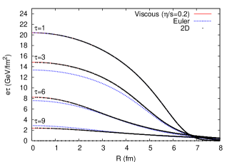
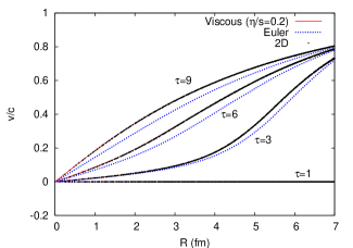
In order to demonstrate the robustness of the above algorithm in two dimensions we compare the results from the 2D numerical solution for central collisions with the corresponding 1D result. In fig. 12 the solid red line shows the result of the energy density per unit rapidity from the 1D case using $\eta/s=0.2$. For reference the ideal result is shown by the dotted blue line. The black points plotted on top of the red curve shows the corresponding result for the 2D case. The difference between the two cases is small as expected. The scatter in the black points gives a qualitative idea of the error due to the use of a rectangular grid. Fig. 12 shows the analogous figure for the transverse velocity.

Figure 12: Scatterplot of the energy density per unit rapidity (left) and of the transverse velocity (right).

D.2 Gradients

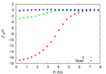
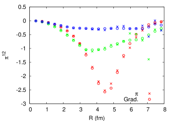
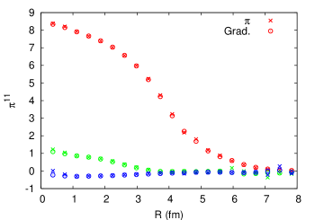
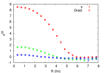
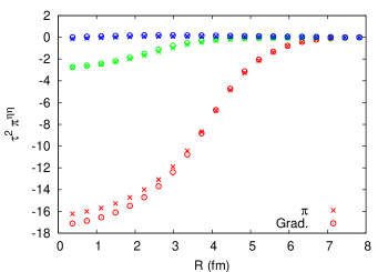
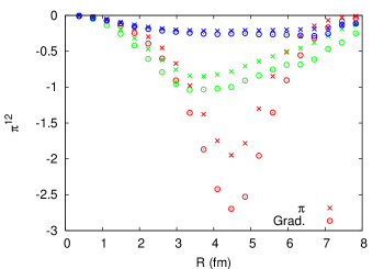
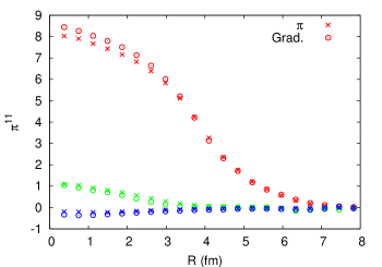
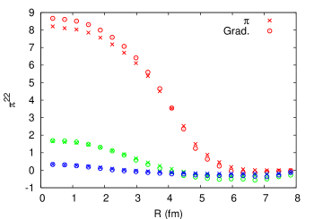
It was discussed in the text that Lindblom Lindblom found an important result regarding the form of the auxillary tensor. In a large class of causal dissipative theories the physical fluid states must relax to a state that is indistinguishable from the Navier-Stokes form. The time scale that which this occurs in on the order of the microscopic particle interaction time.

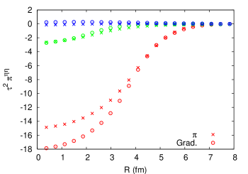
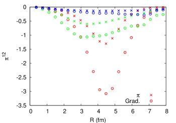
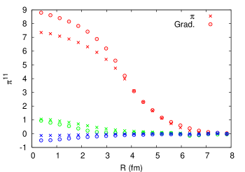
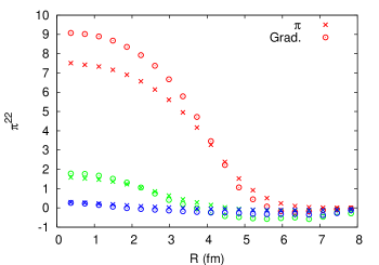
We therefore should check that the viscous stress tensor $\pi^{\mu\nu}$ as computed from the auxiliary tensor $c^{\mu\nu}$ agrees with the stress tensor computed from the gradients of the velocity field. This is shown for various components of $\pi^{\mu\nu}$ from simulations with viscosity of $\eta/s=10^{-6},0.05,0.2$ in figs. 13-15.

   

   

Figure 13: (Color online) Comparison of viscous stress tensor $\pi^{\mu\nu}$ (crosses) versus its explicit calculation from the gradient of the velocity fields (open circles) for $\eta/s=10^{-6}$ for $\tau=2$ (red), $\tau=4$ (green), and $\tau=6$ (blue). All quantities are scaled by $\eta/s$ and were generated from a slice at $30^{\circ}$ in the transverse plane for Au-Au collisions at b=6.5 fm.

   

   

Figure 14: (Color online) Same as fig. 13 except for $\eta/s=0.05$.

   

   

Figure 15: (Color online) Same as fig. 13 except for $\eta/s=0.2$.

References

- (1) M. Grmela, H.C. Öttinger, Phys. Rev. E 56, 6620 (1997). H.C. Öttinger, M. Grmela, Phys. Rev. E 56, 6633 (1997). H.C. Öttinger, Phys. Rev. E 57, 1416 (1993).
- (2) J. Adams et al. [STAR Collaboration], Nucl. Phys. A 757, 102 (2005) [arXiv:nucl-ex/0501009].
- (3) K. Adcox et al. [PHENIX Collaboration], Nucl. Phys. A 757, 184 (2005) [arXiv:nucl-ex/0410003].
- (4) T. Hirano and Y. Nara, Nucl. Phys. A 743, 305 (2004) [arXiv:nucl-th/0404039].
- (5) D. Teaney, J. Lauret and E. V. Shuryak, arXiv:nucl-th/0110037. ibid, Phys. Rev. Lett. 86, 4783 (2001)
- (6) P. F. Kolb, P. Huovinen, U. W. Heinz and H. Heiselberg, Phys. Lett. B 500, 232 (2001) [arXiv:hep-ph/0012137].
- (7) P. Huovinen, P. F. Kolb, U. W. Heinz, P. V. Ruuskanen and S. A. Voloshin, Phys. Lett. B 503, 58 (2001) [arXiv:hep-ph/0101136].
- (8) C. Nonaka and S. A. Bass, Phys. Rev. C 75, 014902 (2007)
- (9) P. Danielewicz and M. Gyulassy, Phys. Rev. D 31, 53 (1985).
- (10) H. J. Drescher, A. Dumitru, C. Gombeaud and J. Y. Ollitrault, Phys. Rev. C 76, 024905 (2007) [arXiv:0704.3553 [nucl-th]].
- (11) P. Petreczky and D. Teaney, Phys. Rev. D 73, 014508 (2006) [arXiv:hep-ph/0507318].
- (12) G. Aarts and J. M. Martinez Resco, JHEP 0204, 053 (2002) [arXiv:hep-ph/0203177]. Meyer:2007ic
- (13) G. Aarts, C. Allton, J. Foley, S. Hands and S. Kim, Phys. Rev. Lett. 99, 022002 (2007) [arXiv:hep-lat/0703008].
- (14) H. B. Meyer, arXiv:0704.1801 [hep-lat].
- (15) P. Arnold, G. D. Moore and L. G. Yaffe, JHEP 0305, 051 (2003) [arXiv:hep-ph/0302165].
- (16) G. Baym, H. Monien, C. J. Pethick and D. G. Ravenhall, Phys. Rev. Lett. 64 (1990) 1867.
- (17) G. Policastro, D. T. Son and A. O. Starinets, Phys. Rev. Lett. 87, 081601 (2001) [arXiv:hep-th/0104066].
- (18) P. Kovtun, D. T. Son and A. O. Starinets Phys. Rev. Lett. 94, 111601 (2005 [arXiv:hep-th/0405231]
- (19) D. Molnar and M. Gyulassy, Nucl. Phys. A 697, 495 (2002) [Erratum-ibid. A 703, 893 (2002)] [arXiv:nucl-th/0104073].
- (20) Z. Xu and C. Greiner, Phys. Rev. C 71, 064901 (2005) [arXiv:hep-ph/0406278].
- (21) D. Teaney, Phys. Rev. C 68, 034913 (2003) [arXiv:nucl-th/0301099].
- (22) H. Song and U. W. Heinz (2007), arXiv:0709.0742 [nucl-th].
- (23) P. Romatschke and U. Romatschke, arXiv:0706.1522 [nucl-th].
- (24) L. D. Landau and E. M. Lifshitz, Fluid Mechanics (Pergamon Press, London, 1959).
- (25) W. Hiscock, L. Lindblom, Phys. Rev. D31, 725 (1985).
- (26) W. Israel, Ann. Phys. 100 (1976) 310; W. Israel and J.M. Stewart, Phys. Lett. 58A (1976) 213.
- (27) W. Israel and J. M. Stewart, Annals Phys. 118, 341 (1979).
- (28) R. Geroch and L. Lindblom, Phys. Rev. D 41, 1855 (1990).
- (29) D. Pavón, D. Jou and J. Casas-Vásquez, Ann. Inst. Henri Poincaré, Sect. A 36, 79 (1982).
- (30) H. C. Öttinger, Physica A 254 (1998) 433-450.
- (31) R. Geroch and L. Lindblom, Annals. Phys. 207, 394 (19901.
- (32) Lee Lindblom, arXiv:gr-qc:9508058.
- (33) D. Forster, Hydrodynamics, Fluctuations, Broken Symmetry, and Correlation Functions, Perseus Books (1990).
- (34) D. Teaney, Phys. Rev. D 74, 045025 (2006) [arXiv:hep-ph/0602044].
- (35) Azwinndini Muronga Phys. Rev. C 69 034903, (2004); Phys. Rev. C 76, 014909 (2007).
- (36) R. Baier, P. Romatschke, and U. A. Wiedemann, Phys. Rev. C 73, 064903 (2006).
- (37) T. Koide, G. S. Denicol, Ph. Mota and T. Kodama, Phys. Rev. C 75, 034909 (2007) [arXiv:hep-ph/0609117].
- (38) P. Espanol, M. Serrano, H. C. Ottinger, Phys. Rev. Lett. 83, 4542 (1999).
- (39) S. Gavin and M. Abdel-Aziz, Phys. Rev. Lett. 97, 162302 (2006) [arXiv:nucl-th/0606061].
- (40) U. Heinz, H. Song and A. K. Chaudhuri, Phys. Rev. C 73 034904, (2006).
- (41) A. K. Chaudhuri, arXiv:nucl-th/0703027; arXiv:nucl-th/0703029; arXiv:0704.0134.
- (42) J. D. Bjorken, Phys. Rev. D 27, 140 (1983).
- (43) M. Prakash, M. Prakash, R. Venugopalan and G. Welke, Phys. Rept. 227, 321 (1993).
- (44) D. Kharzeev and K. Tuchin arXiv:0705.4280 [hep-ph]
- (45) L. Pareschi, SIAM J. Number. Anal 39 (2001). pp. 1395-1417.
- (46) Derek Teaney, J. Phys. G 30 S1247-S1250 (2004).
- (47) P. F. Kolb, J. Sollfrank, and U. Heinz, Phys. Rev. C 65, 054909 (2000).
- (48) Jean-Yves Ollitrault, Phys. Rev. D 46, 229-245 (1992).
- (49) J. P. Bondorf, S. I. A. Garpman and J. Zimanyi, Nucl. Phys. A 296, 320 (1978).
- (50) U. W. Heinz, K. S. Lee and M. J. Rhoades-Brown, Phys. Rev. Lett. 58, 2292 (1987).
- (51) C. M. Hung and E. V. Shuryak, Phys. Rev. C 57, 1891 (1998) [arXiv:hep-ph/9709264].
- (52) F. Reif, ”Fundamentals of Statistical Physics”, McGraw-Hill (1965)
- (53) F. Cooper and G. Frye, Phys. Rev. D. 10, 186 (1974).
- (54) T. Hirano, U. W. Heinz, D. Kharzeev, R. Lacey and Y. Nara, Phys. Lett. B 636, 299 (2006) [arXiv:nucl-th/0511046].
- (55) L. P. Kadanoff and P. C. Martin, Ann. Phys. 24, 419 (1963).
- (56) Derek Teaney, Phys. Rev. D 74, 045025 (2006).
- (57) P. Petreczky and D. Teaney, Phys. Rev. D 73, 014508 (2006).
- (58) J. Adams et al. [STAR Collaboration], Phys. Rev. C 72, 014904 (2005) [arXiv:nucl-ex/0409033].
- (59) R. Baier and P. Romatschke, Eur. Phys. J. C 51, 677 (2007) [arXiv:nucl-th/0610108].
- (60) P. Romatschke, Eur. Phys. J. C 52, 203 (2007) [arXiv:nucl-th/0701032].
- (61) Peter Arnold, Guy D. Moore, and Laurence G. Yaffe, J. High Energy Phys. 11, 001 (2000).