Elliptic and triangular flow in event-by-event (3+1)D viscous hydrodynamics

Abstract

We present results for the elliptic and triangular flow coefficients $v_{2}$ and $v_{3}$ in Au+Au collisions at $\sqrt{s}=200A\,{\rm GeV}$ using event-by-event 3+1D viscous hydrodynamic simulations. We study the effect of initial state fluctuations and finite viscosities on the flow coefficients $v_{2}$ and $v_{3}$ as functions of transverse momentum and pseudo-rapidity. Fluctuations are essential to reproduce the measured centrality dependence of elliptic flow. We argue that simultaneous measurements of $v_{2}$ and $v_{3}$ can determine $\eta/s$ more precisely.

Fluctuating initial conditions for hydrodynamic simulations of heavy-ion collisions have been argued to be very important for the exact determination of collective flow observables and to describe specific features of multi-particle correlation measurements in heavy-ion collisions at Brookhaven National Laboratory’s Relativistic Heavy-Ion Collider (RHIC) Adare et al. (2008); Abelev et al. (2009a); Alver et al. (2010a, b); Abelev et al. (2009b); Miller and Snellings (2003); Broniowski et al. (2007); Hirano and Nara (2009); Takahashi et al. (2009); Andrade et al. (2010); Alver and Roland (2010); Werner et al. (2010); Holopainen et al. (2010); Alver et al. (2010c); Petersen et al. (2010). Both long-range correlations in pseudo-rapidity and double-peak structures on the away-side in $\Delta\eta_{p}$-$\Delta\phi$-correlations have been reproduced using initial states with fluctuations in the transverse plane, extending as flux-tubes along the beam-line Takahashi et al. (2009); Andrade et al. (2010); Alver and Roland (2010); Alver et al. (2010c).

In this work we report on results for both elliptic and triangular flow obtained with an event-by-event 3+1D relativistic hydrodynamic simulation, an extension of music Schenke et al. (2010), including shear viscosity. We first briefly describe the inclusion of viscosity and leave a more detailed description to a forthcoming work.

In the first order formalism for viscous hydrodynamics, the stress-energy tensor is decomposed into

$$T_{\rm 1st}^{\mu\nu}=T^{\mu\nu}_{\rm id}+S^{\mu\nu}\,,$$ (1)

where

$$T_{\rm id}^{\mu\nu}=(\epsilon+{\cal P})u^{\mu}u^{\nu}-{\cal P}g^{\mu\nu}$$ (2)

is the ideal fluid part with flow velocity $u^{\mu}$, local energy density $\epsilon$ and local pressure ${\cal P}$. The flow velocity is defined as the time-like eigenvector of $T^{\mu\nu}_{\rm id}$

$$T^{\mu\nu}_{\rm id}u_{\nu}=-\epsilon u^{\nu}$$ (3)

with the normalization $u^{\nu}u_{\nu}=1$ and the pressure is determined by the equation of state as a function of $\epsilon$.

The viscous part of the stress energy tensor in the first-order approach is given by

$$S^{\mu\nu}=\eta\left(\nabla^{\mu}u^{\nu}+\nabla^{\nu}u^{\mu}-{2\over 3}\Delta^{\mu\nu}\nabla_{\alpha}u^{\alpha}\right)$$ (4)

where $\Delta^{\mu\nu}=g^{\mu\nu}-u^{\mu}u^{\nu}$ is the local 3-metric and $\nabla^{\mu}=\Delta^{\mu\nu}\partial_{\nu}$ is the local space derivative. Note that $S^{\mu\nu}$ is transverse with respect to the flow velocity since $\Delta^{\mu\nu}u_{\nu}=0$ and $u^{\nu}u_{\nu}=1$. Hence, $u^{\mu}$ is also an eigenvector of the whole stress-energy tensor with the same eigenvalue $\epsilon$.

This form of viscous hydrodynamics is conceptually simple. However, this Navier-Stokes form is known to introduce unphysical superluminal signals. There are several remedies for this problem Israel (1976); Stewart (1977); Israel and Stewart (1979); Grmela and Ottinger (1997); Muronga (2002), all of them employing the second order formalism. In this work, we use a variant of the Israel-Stewart formalism derived in Baier et al. (2008), where the stress-energy tensor is decomposed as

$${\cal T}^{\mu\nu}=T^{\mu\nu}_{\rm id}+W^{\mu\nu}\,.$$ (5)

The evolution equations are $\partial_{\mu}{\cal T}^{\mu\nu}=0$ and

$$\Delta^{\mu}_{\alpha}\Delta^{\nu}_{\beta}{u^{\sigma}\partial_{\sigma}}W^{\alpha\beta}=-{1\over\tau_{\pi}}\left(W^{\mu\nu}-S^{\mu\nu}\right)-{4\over 3}W^{\mu\nu}(\partial_{\alpha}u^{\alpha})\,.$$ (6)

In the $\tau,\eta_{s}$ coordinate system we use, these equations can be re-written as hyperbolic equations with sources

$$\partial_{a}T_{\rm id}^{ab}=-\partial_{a}W^{ab}+F^{b}$$ (7)

and

$$\partial_{a}(u^{a}W^{cd})=-(1/\tau_{\pi})(W^{cd}-S^{cd})+G^{cd}$$ (8)

where $F^{b}$ and $G^{cd}$ contain terms introduced by the coordinate change from $t,z$ to $\tau,\eta_{s}$ as well as those introduced by the projections in Eq.(6).

Our approach to solve these hyperbolic equations relies on the Kurganov-Tadmor (KT) scheme Kurganov and Tadmor (2000); Naidoo and Baboolal (2004), together with Heun’s method to solve resulting ordinary differential equations. For details, see Schenke et al. (2010). The main difference between the method employed here and the method used to solve ideal hydrodynamics in Schenke et al. (2010) is the appearance of time-derivatives in the source term. These are handled with the first order approximation $\dot{g}(\tau_{n})=(g(\tau_{n})-g(\tau_{n-1}))/\Delta\tau$ in the first step of the Heun method, and in the second step we use $\dot{g}(\tau_{n})=(g^{*}(\tau_{n+1})-g(\tau_{n}))/\Delta\tau$ where $g^{*}(\tau_{n+1})$ is the result from the first step.

As in most Eulerian algorithms, ours also suffers from numerical instability when the density becomes small while the flow velocity becomes large. Fortunately this happens late in the evolution of the system. Regularizing such instability has no strong effects on the observables we are interested in. Some ways of handling this are known (for instance see Ref.Duez et al. (2004)).

Figure 1: (Color online) Energy density distribution in the transverse plane for one event with $b=2.4\,{\rm fm}$ at the initial time (left), and after $\tau=6\,{\rm fm}/c$ for the ideal case (middle) and with $\eta/s=0.16$ (right).

In this study, we found that setting the local viscosity to zero when finite viscosity causes negative pressure in the cell as advocated in Duez et al. (2004) and reducing the ideal part by 5 % works well to stabilize the calculations without introducing spurious effects.

While in standard hydrodynamic simulations with averaged initial conditions all odd flow coefficients vanish by definition, fluctuations generate triangular flow $v_{3}$ as a response to the finite initial triangularity.

We follow Petersen et al. (2010) and define an event plane through the angle

$$\psi_{n}=\frac{1}{n}\arctan\frac{\langle p_{T}\sin(n\phi)\rangle}{\langle p_{T}\cos(n\phi)\rangle}\,,$$ (9)

where the weight $p_{T}$ is chosen for best accuracy Poskanzer and Voloshin (1998). Then, the flow coefficients can be computed using

$$v_{n}=\langle\cos(n(\phi-\psi_{n}))\rangle\,.$$ (10)

The initialization of the energy density is done using a Glauber Monte-Carlo model (see Miller et al. (2007)): Before the collision the density distribution of the two nuclei is described by a Woods-Saxon parametrization, which we sample to determine the positions of individual nucleons. The impact parameter is sampled from the distribution $P(b)db=2bdb/(b_{\rm max}^{2}-b_{\rm min}^{2})$, where $b_{\rm min}$ and $b_{\rm max}$ depend on the given centrality class. Then we determine the distribution of binary collisions and wounded nucleons. Two nucleons are assumed to collide if their relative transverse distance is less than $D=\sqrt{\sigma_{NN}/\pi}$, where $\sigma_{NN}$ is the inelastic nucleon-nucleon cross-section, which at top RHIC energy of $\sqrt{s}=200A\,{\rm GeV}$ is $\sigma_{NN}=42\,{\rm mb}$. The energy density is distributed proportionally to the wounded nucleon distribution. For every wounded nucleon we add a contribution to the energy density with Gaussian shape (in $x$ and $y$) and width $\sigma_{0}=0.4\,{\rm fm}$. In the rapidity direction, we assume the energy density to be constant on a central plateau and fall like half-Gaussians at large $|\eta_{s}|$ (see Schenke et al. (2010)). This procedure generates flux-tube like structures compatible with measured long-range rapidity correlations Jacobs (2005); Wang (2004); Adams et al. (2005a). The absolute normalization is determined by demanding that the obtained total multiplicity distribution reproduces the experimental data.

As equation of state we employ the parametrization “s95p-v1” from Huovinen and Petreczky (2010), obtained from interpolating between lattice data and a hadron resonance gas.

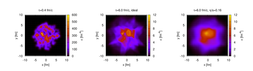
In Fig. 1 we show the energy density distribution in the transverse plane for an event with impact parameter $b=2.4\,{\rm fm}$ at the initial time $\tau_{0}=0.4\,{\rm fm}/c$ and at time $\tau=6\,{\rm fm}/c$ for $\eta/s=0$ and $\eta/s=0.16$. This clearly shows the effect of dissipation.

We perform a Cooper-Frye freeze-out using

$$E\frac{dN}{d^{3}p}=\frac{dN}{dyp_{T}dp_{T}d\phi_{p}}=g_{i}\int_{\Sigma}f(u^{\mu}p_{\mu})p^{\mu}d^{3}\Sigma_{\mu}\,,$$ (11)

where $g_{i}$ is the degeneracy of particle species $i$, and $\Sigma$ the freeze-out hyper-surface. In the ideal case the distribution function is given by

$$f(u^{\mu}p_{\mu})=f_{0}(u^{\mu}p_{\mu})=\frac{1}{(2\pi)^{3}}\frac{1}{\exp((u^{\mu}p_{\mu}-\mu_{i})/T_{\rm FO})\pm 1}\,,$$ (12)

where $\mu_{i}$ is the chemical potential for particle species $i$ and $T_{\rm FO}$ is the freeze-out temperature. In the finite viscosity case we include viscous corrections to the distribution function, $f=f_{0}+\delta f$, with

$$\delta f=f_{0}(1\pm f_{0})p^{\alpha}p^{\beta}W_{\alpha\beta}\frac{1}{2(\epsilon+\mathcal{P})T^{2}}\,,$$ (13)

where $W$ is the viscous correction introduced in Eq. (5). Note that the choice $\delta f\sim p^{2}$ is not unique Dusling et al. (2010).

The algorithm used to determine the freeze-out surface $\Sigma$ has been presented in Schenke et al. (2010). It is very efficient in determining the freeze-out surface of a system with fluctuating initial conditions. To demonstrate this, we present the freeze-out surface in the $x$-$\tau$-plane in the vicinity of $y=0\,{\rm fm}$ and $\eta_{s}=0$ for two different initial distributions compared to that for an averaged initial condition in Fig. 2. The arrows are projections of the normal vector on the hyper-surface element onto the $x$-$\tau$ plane.

We include resonances up to the $\phi$-meson. We found that the pseudorapidity dependence of both $v_{2}$ and $v_{3}$ is affected notably by the inclusion of resonance decays, improving the agreement of $v_{2}(\eta_{p})$ with data significantly. $v_{2}(p_{T})$ at midrapidity is almost unaffected by the resonances while $v_{3}(p_{T})$ is reduced by approximately 20-30%.

Figure 2: (Color online) Freeze-out surfaces for two different events (red and yellow) compared to that for the averaged initial condition (gray).

Figure 3: (Color online) Charged hadron $v_{2}$ for different centralities as a function of transverse momentum for averaged initial conditions (avg) and event-by-event simulations (e-b-e) using different viscosity to entropy density ratios compared to STAR Adams et al. (2005b) and PHENIX Adare et al. (2010) data.

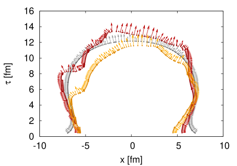
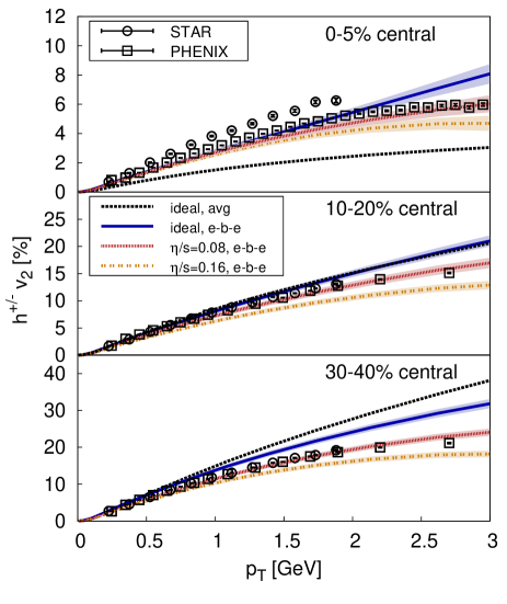
Fig. 3 shows the elliptic flow $v_{2}$ for charged hadrons as a function of transverse momentum obtained from an averaged initial condition in the ideal case and for an average over 100 individual events for $\eta/s\in\{0,0.08,0.16\}$. We compare to data from STAR Adams et al. (2005b) and PHENIX Adare et al. (2010). The used minimal, maximal, and average impact parameter for each centrality class are given in Table 1 .

centrality [%]	$b_{\rm min}$ [fm]	$b_{\rm max}$ [fm]	$\langle b\rangle$ [fm]
0-5	0	3.37	2.24
10-20	4.75	6.73	5.78
15-25	5.83	7.53	6.7
30-40	8.23	9.5	8.87

Table 1: Used impact parameters.

While in the most central collisions fluctuations increase $v_{2}$ compared to the case with averaged initial conditions, for 10-20% central collisions the difference is negligible and for 30-40% central collisions fluctuations reduce the elliptic flow. The increase for central collisions is easy to understand since we are now determining $v_{2}$ in every event. Single events have a larger anisotropy with respect to the event-plane than the average with respect to the reaction plane, hence increasing the obtained $v_{2}$. This effect decreases with increasing centrality eventually making the event-by-event $v_{2}$ smaller compared to the averaged initial condition case. This can be understood by the fact that for more peripheral collisions, lumps in the initial condition tend not to align perfectly with the statistically determined event plane.

Viscosity reduces the elliptic flow for all centralities as also found in (2+1)-dimensional simulations Romatschke and Romatschke (2007); Dusling and Teaney (2008); Molnar and Huovinen (2008); Song and Heinz (2008).

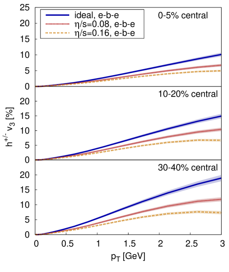
Triangular flow $v_{3}$ as a function of transverse momentum is shown in Fig. 4. $v_{3}$ depends less strongly on the centrality than $v_{2}$ since it is completely fluctuation driven. It is largest for an ideal fluid and reduces similarly to $v_{2}$ with increasing viscosity of the medium.

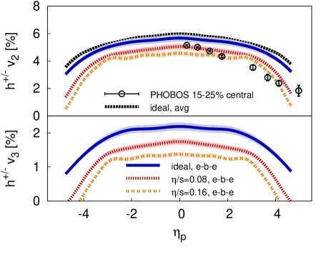
The upper panel of Fig. 5 shows the pseudo-rapidity dependence of $v_{2}$ for 15-25% central collisions compared to PHOBOS data Back et al. (2005). A reduction of elliptic flow with increasing viscosity is visible, particularly for large pseudo-rapidities $|\eta_{p}|$, which has been anticipated Bozek and Wyskiel (2009); Schenke et al. (2010). In the lower panel of Fig. 5 we present the $\eta_{p}$-dependence of $v_{3}$. Again, the decrease of $v_{3}$ with increasing viscosity is visible, being strongest for large $|\eta_{p}|$.

We presented the elliptic and triangular flow coefficients obtained with an event-by-event analysis using (3+1)-dimensional relativistic viscous hydrodynamics. Charged hadron elliptic flow around midrapidity is well described for a wide range of centralities when using $\eta/s=0.08$, the conjectured lower bound from AdS/CFT Kovtun et al. (2005). A similarly small value was found in a parton cascade model based on perturbative QCD Xu et al. (2008). Larger viscosities underestimate elliptic flow. Shear viscosity reduces $v_{2}$ especially for larger pseudo-rapidities, however, the data is still overestimated away from midrapidity. Triangular flow has a weaker dependence on centrality. We determined its transverse momentum and pseudo-rapidity dependence, as well as its dependence on $\eta/s$. When triangular flow data becomes available, combined analyses of both $v_{2}$ and $v_{3}$ can make an accurate determination of the shear-viscosity possible.

Figure 4: (Color online) Charged hadron $v_{3}$ for different centralities as a function of $p_{T}$ for event-by-event simulations using different viscosity to entropy density ratios.

Figure 5: (Color online) Charged hadron $v_{2}$ and $v_{3}$ as a function of pseudo-rapidity for event-by-event simulations using different viscosity to entropy density ratios.

Acknowledgments We thank Pasi Huovinen and Paul Romatschke for helpful comments and Todd Springer for fruitful discussions and checks. This work was supported in part by the Natural Sciences and Engineering Research Council of Canada. B. S. gratefully acknowledges a Richard H. Tomlinson Postdoctoral Fellowship by McGill University.

References

- Adare et al. (2008) A. Adare et al. (PHENIX), Phys. Rev. C78, 014901 (2008).
- Abelev et al. (2009a) B. I. Abelev et al. (STAR), Phys. Rev. Lett. 102, 052302 (2009a).
- Alver et al. (2010a) B. Alver et al. (PHOBOS), Phys. Rev. C81, 024904 (2010a).
- Alver et al. (2010b) B. Alver et al. (PHOBOS), Phys. Rev. Lett. 104, 062301 (2010b).
- Abelev et al. (2009b) B. I. Abelev et al. (STAR), Phys. Rev. C80, 064912 (2009b).
- Miller and Snellings (2003) M. Miller and R. Snellings (2003), eprint nucl-ex/0312008.
- Broniowski et al. (2007) W. Broniowski et al., Phys. Rev. C76, 054905 (2007).
- Hirano and Nara (2009) T. Hirano and Y. Nara, Nucl. Phys. A830, 191c (2009).
- Takahashi et al. (2009) J. Takahashi et al., Phys. Rev. Lett. 103, 242301 (2009).
- Andrade et al. (2010) R. Andrade et al., J. Phys. G37, 094043 (2010).
- Alver and Roland (2010) B. Alver and G. Roland, Phys. Rev. C81, 054905 (2010).
- Werner et al. (2010) K. Werner, I. Karpenko, T. Pierog, M. Bleicher, and K. Mikhailov (2010), eprint arXiv:1004.0805.
- Holopainen et al. (2010) H. Holopainen, H. Niemi, and K. J. Eskola (2010), eprint arXiv:1007.0368.
- Alver et al. (2010c) B. Alver et al. (2010c), eprint arXiv:1007.5469.
- Petersen et al. (2010) H. Petersen et al. (2010), eprint arXiv:1008.0625.
- Schenke et al. (2010) B. Schenke, S. Jeon, and C. Gale, Phys. Rev. C82, 014903 (2010).
- Israel (1976) W. Israel, Ann. Phys. 100, 310 (1976).
- Stewart (1977) J. Stewart, Proc.Roy.Soc.Lond. A357, 59 (1977).
- Israel and Stewart (1979) W. Israel and J. M. Stewart, Ann. Phys. 118, 341 (1979).
- Grmela and Ottinger (1997) M. Grmela and H. C. Ottinger, Phys. Rev. E56, 6620 (1997).
- Muronga (2002) A. Muronga, Phys. Rev. Lett. 88, 062302 (2002).
- Baier et al. (2008) R. Baier, P. Romatschke, D. T. Son, A. O. Starinets, and M. A. Stephanov, JHEP 04, 100 (2008).
- Kurganov and Tadmor (2000) A. Kurganov and E. Tadmor, Journal of Computational Physics 160, 214 (2000).
- Naidoo and Baboolal (2004) R. Naidoo and S. Baboolal, Future Gener. Comput. Syst. 20, 465 (2004).
- Duez et al. (2004) M. D. Duez et al., Phys. Rev. D69, 104030 (2004).
- Poskanzer and Voloshin (1998) A. M. Poskanzer and S. A. Voloshin, Phys. Rev. C58, 1671 (1998).
- Miller et al. (2007) M. L. Miller, K. Reygers, S. J. Sanders, and P. Steinberg, Ann. Rev. Nucl. Part. Sci. 57, 205 (2007).
- Jacobs (2005) P. Jacobs, Eur. Phys. J. C43, 467 (2005).
- Wang (2004) F. Wang (STAR), J. Phys. G30, S1299 (2004).
- Adams et al. (2005a) J. Adams et al. (STAR), Phys. Rev. Lett. 95, 152301 (2005a).
- Huovinen and Petreczky (2010) P. Huovinen and P. Petreczky, Nucl. Phys. A837, 26 (2010).
- Dusling et al. (2010) K. Dusling, G. D. Moore, and D. Teaney, Phys. Rev. C81, 034907 (2010).
- Adams et al. (2005b) J. Adams et al. (STAR), Phys. Rev. C72, 014904 (2005b).
- Adare et al. (2010) A. Adare et al. (PHENIX), Phys. Rev. Lett. 105, 062301 (2010).
- Romatschke and Romatschke (2007) P. Romatschke and U. Romatschke, Phys. Rev. Lett. 99, 172301 (2007).
- Dusling and Teaney (2008) K. Dusling and D. Teaney, Phys. Rev. C77, 034905 (2008).
- Molnar and Huovinen (2008) D. Molnar and P. Huovinen, J. Phys. G35, 104125 (2008).
- Song and Heinz (2008) H. Song and U. W. Heinz, Phys. Rev. C78, 024902 (2008).
- Back et al. (2005) B. B. Back et al. (PHOBOS), Phys. Rev. C72, 051901 (2005).
- Bozek and Wyskiel (2009) P. Bozek and I. Wyskiel, PoS EPS-HEP-2009, 039 (2009).
- Kovtun et al. (2005) P. Kovtun et al., Phys. Rev. Lett. 94, 111601 (2005).
- Xu et al. (2008) Z. Xu et al., Phys. Rev. Lett. 101, 082302 (2008).