Emergence of steady and oscillatory localized structures in a phytoplankton–nutrient model

Abstract

Co-limitation of marine phytoplankton growth by light and nutrient, both of which are essential for phytoplankton, leads to complex dynamic behavior and a wide array of coherent patterns. The building blocks of this array can be considered to be deep chlorophyll maxima, or DCMs, which are structures localized in a finite depth interior to the water column. From an ecological point of view, DCMs are evocative of a balance between the inflow of light from the water surface and of nutrients from the sediment. From a (linear) bifurcational point of view, they appear through a transcritical bifurcation in which the trivial, no-plankton steady state is destabilized. This article is devoted to the analytic investigation of the weakly nonlinear dynamics of these DCM patterns, and it has two overarching themes. The first of these concerns the fate of the destabilizing stationary DCM mode beyond the center manifold regime. Exploiting the natural singularly perturbed nature of the model, we derive an explicit reduced model of asymptotically high dimension which fully captures these dynamics. Our subsequent and fully detailed study of this model—which involves a subtle asymptotic analysis necessarily transgressing the boundaries of a local center manifold reduction—establishes that a stable DCM pattern indeed appears from a transcritical bifurcation. However, we also deduce that asymptotically close to the original destabilization, the DCM looses its stability in a secondary bifurcation of Hopf type. This is in agreement with indications from numerical simulations available in the literature. Employing the same methods, we also identify a much larger DCM pattern. The development of the method underpinning this work—which, we expect, shall prove useful for a larger class of models—forms the second theme of this article.

1 Introduction

Phytoplanktonic photosynthesis provides the major biological component of the transport mechanism carrying atmospheric carbon dioxide into the deep ocean. Concurrently, plankton forms the basis of the aquatic food chain. As a consequence, phytoplankton growth and decay plays a crucial role in understanding climate dynamics [10] and forms an integral part of oceanographic research. Conversely, climate changes—such as global temperature variations—have a direct impact on the aquatic ecosystem and thus also on phytoplankton [3, 22]: there is a subtle and under-explored interplay between the dynamics of phytoplankton concentrations and climate variability. At the same time, phytoplankton concentrations exhibit surprisingly rich spatio-temporal dynamics. The character of those dynamics is determined in an intricate fashion by (changes in) the external conditions, see [15] and the references therein. The building blocks for the observed complex patterns are deep chlorophyll maxima (DCMs) or phytoplankton blooms, in which the phytoplankton concentration exhibits a maximum at a certain, well-defined depth of the basin. These patterns are the manifestation of a fundamental balance between the supply of light from the surface and of nutrients from the depths of the basin. For the simplest models, in which spatiotemporal fluctuations in the nutrient concentration are omitted (eutrophic environment), it has been shown that there can only be a stationary global attractor [17]. In particular, if the trivial state (no phytoplankton) is unstable, then there can only be a stationary globally attracting phytoplankton bloom with its maximum either at the surface (a surface layer), at the bottom (a benthic layer, BL), or in between (a DCM) [9, 12, 13, 17]. This is no longer the case in coupled phytoplankton–nutrient systems (oligotrophic environment), although DCMs do tend to appear in those systems, also, for certain parameter combinations [6, 7, 11, 13, 16, 18]. The detailed numerical studies reported in [15], however, show that the appearance of a DCM only triggers a complex sequence of bifurcations: as parameters vary, a DCM may be time-periodic, undergo a sequence of period doubling bifurcations, and eventually behave chaotically.

In this paper, we focus on the effect that varying environmental conditions, and in particular nutrient levels at the ocean bed, have on the dynamics generated by the one-dimensional model for phytoplankton ($W$)–nutrient ($N$) interactions originally introduced in [15],

$$\left\{\begin{array}[]{l}W_{t}=D\,W_{zz}-V\,W_{z}+\left[\mu\,P(L,N)-l\right]W,\\ N_{t}=D\,N_{zz}-Y^{-1}\,\mu\,P(L,N)\,W.\end{array}\right.$$ (1.1)

In this model, the vertical coordinate $z$ measures the depth in a water column spanned by $[0,z_{B}]$, while $W(z,t)$ and $N(z,t)$ are the phytoplankton and nutrient concentrations, respectively, at depth $z$ and time $t$. As in [15, 25], the system is assumed to be in the turbulent mixing regime [9, 13], so that the diffusion coefficient $D$ is identically the same for phytoplankton and nutrient. The phytoplankton is characterized by its sinking speed $V$, its (species-specific) loss rate $l$, its maximum specific production rate $\mu$, and its yield $Y$ on light and nutrient. The model is equipped with natural no-flux boundary conditions at the surface for both phytoplankton and nutrients; the bottom is a source of nutrients but impenetrable for phytoplankton,

$$D\,W_{z}-V\,W|_{z=0,z_{B}}=0,\quad N_{z}|_{z=0}=0,\quad\mbox{and}\quad N|_{z=z_{B}}=N_{B}.$$ (1.2)

The constant nutrient concentration $N_{B}$ will act as the primary bifurcation parameter in this work. The nonlinear expression $P(L,N)$ models phytoplankton growth due to light and nutrient,

$$P(L,N)=\frac{LN}{(L+L_{H})(N+N_{H})},$$ (1.3)

in which $L_{H}$ and $N_{H}$ are the half-saturation constants of light and nutrient, respectively. (See [25] for a short discussion on the nature and specificity of $P(L,N)$.) The light intensity $L$ at depth $z$ and time $t$ is determined by the total amount of planktonic and non-planktonic components in the column $[0,z]$,

$$L(z,t)=L_{I}\,\mathrm{e}^{-K_{bg}z-R\int_{0}^{z}W(s,t)ds}.$$ (1.4)

Hence, the system is non-local—a typical feature of most realistic phytoplankton models. The light intensity term introduces an extra three parameters: $L_{I}$, the intensity of the incident light at the water surface; $K_{bg}$, the light absorption coefficient due to non-planktonic, background components and hence a measure of turbidity; and $R$, the light absorption coefficient due to plankton (self-shading). The first two of these parameters, together with $z_{B}$, $D$, $Y$, and $N_{B}$ quantify the effect that the environment has on the planktonic population. It is by varying these parameters that we examine the effect of changing environmental conditions on plankton.

It is shown in [25] that the system (1.1) has a natural singularly perturbed nature. This can be seen by rescaling time and space via $\tau=\mu\,t$ and $x=z/z_{B}$ and the phytoplankton concentration $W$, nutrient concentration $N$, and light intensity $L$ via

$$\omega^{+}(x,\tau)=\frac{lz_{B}^{2}}{DYN_{B}}W(z,t),\quad\eta(x,\tau)=1-\frac{N(z,t)}{N_{B}},\quad\mbox{and}\quad j(x,\tau)=\frac{L(z,t)}{L_{I}}.$$

Substitution into (1.1) then yields,

$$\begin{array}[]{l}\omega^{+}_{\tau}=\varepsilon\omega^{+}_{xx}-2\sqrt{\varepsilon\mathrm{v}}\,\omega^{+}_{x}+(p(\omega^{+},\eta,x)-\ell)\,\omega^{+},\\ \eta_{\tau}=\varepsilon\left(\eta_{xx}+\ell^{-1}p(\omega^{+},\eta,x)\,\omega^{+}\right),\end{array}$$ (1.5)

with boundary conditions,

$$(\omega^{+}_{x}-2\sqrt{\mathrm{v}/\varepsilon}\,\omega^{+})(0)=(\omega^{+}_{x}-2\sqrt{\mathrm{v}/\varepsilon}\,\omega^{+})(1)=0\quad\mbox{and}\quad\eta_{x}(0)=\eta(1)=0.$$ (1.6)

For realistic choices of the original parameters of (1.1),

$$\varepsilon=\frac{D}{\mu z_{B}^{2}}\approx 10^{-5},$$

cf. [15, 25]. Effectively, $\varepsilon^{1/4}$ characterizes the extent of the zone where DCMs appear relative to the depth of the ocean. In this paper, we follow [25] and treat the parameter $\varepsilon$ as an asymptotically small parameter, i.e., we assume that $0<\varepsilon\ll 1$ so that (1.5) has, indeed, a singularly perturbed character. The nonlinearity $p$ in (1.5) is given by

$$p(\omega^{+},\eta,x)=\frac{1-\eta}{(\eta_{H}+1-\eta)\,(1+j_{H}/j(\omega^{+},x))},$$ (1.7)

with rescaled light intensity

$$j(\omega^{+},x)=\exp\left(-\kappa x-r\int_{0}^{x}\omega^{+}(s,\tau)ds\right).$$ (1.8)

The remaining six rescaled parameters of (1.5),

$$\mathrm{v}=\frac{V^{2}}{4\mu D},\quad\ell=\frac{l}{\mu},\quad j_{H}=\frac{L_{H}}{L_{I}},\quad\eta_{H}=\frac{N_{H}}{N_{B}},\quad\kappa=K_{bg}z_{B},\quad\mbox{and}\quad r=\frac{RDYN_{B}}{lz_{B}},$$ (1.9)

are all considered to be $\Or(1)$ with respect to $\varepsilon$ in the forthcoming analysis (cf. [25]).

Our attempt to comprehend the mechanism underpinning the appearance of phytoplankton patterns, as well as the character of such patterns, begins with the determination of the spectral stability of the trivial steady state $u^{+}=(0,0)^{\rm T}$. At that state, and in terms of the original system (1.1), there is no phytoplankton—$W(z,t)\equiv 0$—and the nutrient concentration remains constant throughout the column—$N(z,t)\equiv N_{B}$, the value at the bottom of the basin (1.2). The system (1.5) may be written compactly in the form

$$u^{+}_{\tau}=\mathcal{T}^{+}(u^{+})=\left(\begin{array}[]{c}\varepsilon\,\omega^{+}_{xx}-2\sqrt{\varepsilon\mathrm{v}}\,\omega^{+}_{x}+(p(\omega^{+},\eta,x)-\ell)\,\omega^{+}\\ \varepsilon\,\eta_{xx}+\varepsilon\,\ell^{-1}\,p(\omega^{+},\eta,x)\,\omega^{+}\end{array}\right),$$ (1.10)

where

$$u^{+}=\left(\begin{array}[]{c}\omega^{+}\\ \eta\end{array}\right).$$

Here, the nonlinear operator $\mathcal{T}^{+}$ is densely defined in ${\rm L}^{2}(0,1)\times{\rm L}^{2}(0,1)$. The associated spectral problem has been investigated in full asymptotic detail in [25], where we worked with the linearization of (1.10) around $u^{+}=(0,0)^{\rm T}$,

$$\mathcal{DT}^{+}=\left(\begin{array}[]{cc}\varepsilon\,\partial_{xx}-2\sqrt{\varepsilon\mathrm{v}}\,\partial_{x}+f-\ell&0\\ \varepsilon\,\ell^{-1}\,f&\varepsilon\,\partial_{xx}\end{array}\right),$$ (1.11)

in which

$$f(x)=\frac{\nu}{1+j_{H}\mathrm{e}^{\kappa x}}\quad\mbox{and}\quad\nu=\frac{1}{1+\eta_{H}}\in(0,1).$$ (1.12)

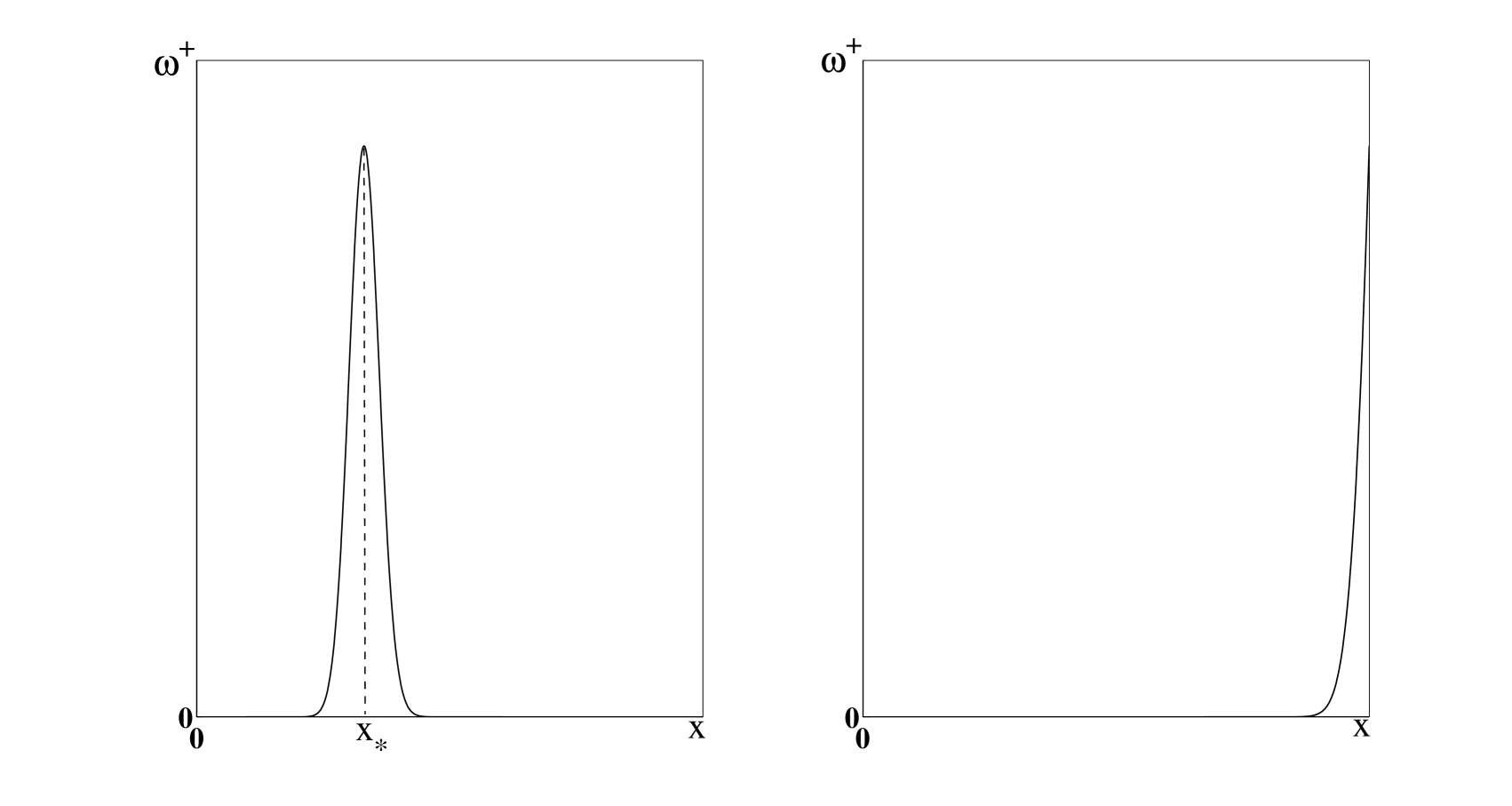
Figure 1: Left panel: a DCM profile for the planktonic component of (1.5)–(1.6). Essentially all plankton is concentrated in an $\Or(\varepsilon^{1/4})$ region around a finite depth ${x_{*}}$. Right panel: a BL profile for the planktonic component of (1.5)–(1.6). Here, essentially all plankton is concentrated in an $\Or(\varepsilon^{1/2})$ region over the depth of the basin.

The spectrum $\sigma(\mathcal{DT}^{+})=\{\nu_{n}\}_{n\geq 0}\cup\{\lambda_{n}\}_{n\geq 0}$ of the operator $\mathcal{DT}^{+}$ consists of two distinct, real parts associated with the two diagonal blocks of $\mathcal{DT}^{+}$, cf. (1.11). Here, the eigenvalues $\nu_{n}=-\varepsilon\,(n+1/2)^{2}\,\pi^{2}$ are negative, independent of all parameters, and associated with the lower block. These eigenvalues, together with the corresponding sinusoidal eigenfunctions $(0,\cos((n+1/2)\pi x))^{\rm T}$, describe nutrient diffusion in the complete absence of phytoplankton. It follows that the spectral stability of the trivial state is governed solely by $\{\lambda_{n}\}_{n\geq 0}$, the set of eigenvalues associated with the upper block. In [25], we identified two different linear destabilization mechanisms. In the regime $\mathrm{v}<f(0)-f(1)$, corresponding to reduced oceanic diffusivity or increased turbidity (cf. (1.9) and (1.12)), the planktonic component $\omega^{+}_{0}$ of the eigenfunction $w_{0}^{+}$ associated with the critical eigenvalue $\lambda_{0}$ has the character of a DCM: $\omega^{+}_{0}$ is localized in an $\Or(\varepsilon^{1/4})$ region centered around a certain depth ${x_{*}}$ at which it attains its maximal value, see Figure 1. This depth can be determined explicitly: to leading order, $f({x_{*}})=f(0)-\mathrm{v}$ [25]. Hence, ${x_{*}}$ increases monotonically from ${x_{*}}=0$ to ${x_{*}}=1$ as $\mathrm{v}$ increases from $\mathrm{v}=0$ to the transitional value $\mathrm{v}=f(0)-f(1)$. In the complementary case $\mathrm{v}>f(0)-f(1)$, corresponding to increased oceanic diffusivity or decreased turbidity, the planktonic component of the critical eigenfunction destabilizing the trivial state has the character of a BL: that is, it increases monotonically with depth and essentially all phytoplankton is concentrated in an $\Or(\varepsilon^{1/2})$ region over the bottom, see again Figure 1.

In this article, we focus exclusively on the regime in which DCMs may appear, i.e., we assume throughout the article that $\mathrm{v}<f(0)-f(1)$. In that regime, we investigate the nature of the bifurcation associated with the destabilization mechanism of DCM type. We know from [25] that, in this case,

$$\lambda_{n}=\lambda_{*}-\varepsilon^{1/3}\sigma_{0}^{2/3}\left|A_{n+1}\right|+\Or(\varepsilon^{1/2}),$$ (1.13)

with

$$\lambda_{*}=f(0)-\ell-\mathrm{v}=\frac{\nu}{1+j_{H}}-\ell-\mathrm{v}$$ (1.14)

and where

$$\sigma_{0}=F^{\prime}(0)=-f^{\prime}(0)=\frac{\kappa\,\nu\,j_{H}}{(1+j_{H})^{2}},\quad\mbox{with}\quad F(x)=f(0)-f(x).$$ (1.15)

Here, $A_{n}<0$ is the $n-$th root of ${\rm Ai}$, the Airy function of the first kind. The bifurcation occurs as $\lambda_{0}$ crosses zero, yielding the bifurcation diagram in the left panel of Figure 2. More specifically, we focus on the (weakly nonlinear) dynamics generated by (1.10) for parameter choices such that

$$\lambda_{0}=\frac{\nu}{1+j_{H}}-\ell-\mathrm{v}-\varepsilon^{1/3}\sigma_{0}^{2/3}\left|A_{1}\right|+\Or(\varepsilon^{1/2})=\varepsilon^{\rho}\Lambda_{0},$$ (1.16)

where $\rho>0$ is fixed and $\Lambda_{0}$ is allowed to be at most logarithmically large with respect to $\varepsilon$. Note that one can tune the appearance of a destabilization of DCM type (i.e., of the simplest phytoplankton pattern) by choosing appropriately the parameters in (1.10); also, that $\lambda_{0}$ depends on all parameters with the exception of $r$, the rescaled self-shading coefficient, see the definitions of $f$ and $\sigma_{0}$ in (1.12) and (1.15). We remark, further, that the parameter $\mathrm{v}$ depends on the diffusion coefficient $D$ (cf. (1.9)), the main parameter varied in [15] and the one that most strongly depends on varying external conditions such as global temperature [22]. Finally, $\Lambda_{0}$ is an increasing function of our bifurcation parameter $N_{B}$ through its dependence on $\nu$, see (1.13)–(1.14) together with the definitions of $\nu$ in (1.12) and of $\eta_{H}$ in (1.9). Based on this final observation, we will often treat $\Lambda_{0}$ as our bifurcation parameter.

The first step in analyzing the dynamics generated by a linear destabilization mechanism is to perform a center manifold analysis to determine the local character of the bifurcation associated with the destabilization (see, for instance, [1, 4]). This is a well-established procedure. In the setting of (1.16), this amounts to assuming that $\lambda_{0}$ is (asymptotically) smaller than all other eigenvalues, and it corresponds to the case $\rho>1$ and $\Lambda_{0}=\Or(1)$. In this regime, the remaining eigenvalues $\{\nu_{n}\}_{n\geq 0}\cup\{\lambda_{n}\}_{n\geq 1}$ are negative and asymptotically larger than $\lambda_{0}$, so that the local flow near the trivial pattern $(0,0)^{\rm T}$ is determined by the flow on the one-dimensional center manifold. The tangent space of this manifold at the trivial steady state is spanned by the critical eigenfunction $w_{0}^{+}$ associated with $\lambda_{0}$. Hence, this flow can be determined by expanding $u^{+}$ as $u^{+}(x,\tau)=\varepsilon^{\rho-1/6}\,\Omega_{0}(\tau)\,w_{0}^{+}(x)+R(x,t)$, with $\Omega_{0}$ being an unknown, time-dependent amplitude and the higher order remainder $R$ encapsulating the component of $u^{+}$ along directions associated with the stable eigenvalues—the additional $1/6$ in the exponent of $\varepsilon$ follows from the projection analysis by which the equation for $\Omega_{0}$ is determined (see below and Section 3). An ODE for the unknown amplitude $\Omega_{0}$ is obtained through a projection procedure which is straightforward but can nevertheless be highly technical, especially in a PDE setting. In the case at hand, this equation reads

$$\dot{\Omega}_{0}=\Lambda_{0}\,\Omega_{0}-a_{000}(0)\,\Omega_{0}^{2},$$ (1.17)

to leading order. Thus, the procedure reveals the existence of a nontrivial fixed point which is stabilized through a standard, co-dimension one transcritical bifurcation. This fixed point corresponds to an asymptotically small DCM pattern, the amplitude of which grows linearly with $\Lambda_{0}$,

$$\omega^{+}(x)\sim\varepsilon^{\rho-1/6}\,\Omega^{*}_{0}\,\omega^{+}_{0}(x),\quad\mbox{with}\ \Omega^{*}_{0}=\frac{\Lambda_{0}}{a_{000}(0)}.$$ (1.18)

In general, one cannot expect to be able to compute the coefficient $a_{000}(0)$ explicitly. Here, we exploit the singularly perturbed nature of (1.10) and the localized character of the eigenfunction $w_{0}^{+}$ to do exactly that; in particular, it follows from the analysis to be presented in this article that

$$a_{000}(0)=(1-\nu)(1-{x_{*}})\,\frac{\sigma_{0}^{1/3}\,f(0)\,\exp(\left|A_{1}\right|^{3/2})}{\left(\left|f^{\prime}({x_{*}})\right|\int_{A_{1}}^{\infty}{\rm Ai}^{2}(s)\,ds\right)^{1/2}}>0,$$ (1.19)

see Section 3. In addition to yielding an explicit, leading order formula for the amplitude of the emerging (stable) DCM, this first result also implies that this DCM is ecologically relevant since the planktonic component of the primary eigenfunction is positive, $\omega^{+}_{0}>0$, and hence also $\omega^{+}>0$ by (1.18)–(1.19).

The main aim of this paper is to develop an analytic approach through which one can go beyond the direct, finite-dimensional center manifold reduction outlined above. The original ideas underlying this approach—namely, the method of weakly nonlinear stability analysis—qualify as classical [23]. However, this particular method does not always provide more insight than the rigorously established center manifold reduction method: for instance, it also reduces the flow to a one-dimensional ODE of the form (1.17). The situation is strikingly different here, as we can exploit the singularly perturbed nature of (1.10), in conjunction with the asymptotic information on the eigenfunctions of $\mathcal{DT}^{+}$ obtained in [25], to study in full analytic detail the case $\lambda_{0}={\cal O}(\varepsilon)$—see Section 4—and even extend our analysis to the regime $\lambda_{0}={\cal O}(\varepsilon\log^{2}\varepsilon)$—see Section 4.5. This way, we can analytically trace the fate of the bifurcating DCM pattern well into the regime where the pattern undergoes secondary and, possibly, even tertiary bifurcations.

For clarity of presentation, we divide the rest of the material in this Introduction into two parts. The first one focuses on the bifurcations undergone by the DCM patterns and on the ecological interpretation of our findings, while the second one focuses on the specifics of the asymptotic method developed in this work.

1.1 The bifurcations of the DCM patterns

The outcome of our asymptotic analysis is summarized in the right panel of Figure 2. The localized DCM that bifurcates as $\lambda_{0}$ crosses zero is a stable attractor of the flow generated by (1.1), for all $\rho>1$ and $\Lambda_{0}={\cal O}(1)$ with respect to $\varepsilon$, cf. (1.16). As we remarked above, the amplitude $\Omega_{0}^{*}$ of this localized DCM, and thus also the biomass associated with it, grows linearly with $\Lambda_{0}$ in that regime, cf. (1.18)–(1.19). Quite remarkably, from the point of view of our weakly nonlinear stability analysis, $\Omega_{0}^{*}$ continues growing linearly with $\Lambda_{0}$ also beyond the region where the center manifold reduction is valid. In particular, (1.18)–(1.19) remain valid in the regime $\rho=1$ and $\Lambda_{0}=\Or(1)$, see (4.9). The corresponding biomass turns out to be

$$\int_{0}^{1}\omega^{+}(x)\,dx=\varepsilon\frac{(1+j_{H})}{(1-\nu)\,\nu\,(1-{x_{*}})}\,\Lambda_{0}=\frac{(1+j_{H})\,\nu-\ell-\mathrm{v}}{(1-\nu)\,(1-{x_{*}})\,(\ell+\mathrm{v})},$$ (1.20)

to leading order. This second result establishes that, in the $\lambda_{0}={\cal O}(\varepsilon)$ regime, the DCM pattern grows with $\nu$ and hence also with $N_{B}$, the primary parameter measuring nutrient availability in the water column (see (1.9) and (1.12)). This fact certainly reinforces our ecological intuition.

The stability properties of the DCM mode corresponding to $\Omega_{0}^{*}$, on the other hand, undergo a drastic change in that same regime. Our rather involved stability analysis of this emergent nontrivial steady state reveals that it becomes unstable, in this same $\lambda_{0}={\cal O}(\varepsilon)$ regime already, as $\Lambda_{0}$ continues to grow and through a standard Hopf bifurcation; this is our third result. The appearance of this secondary bifurcation can be determined explicitly by our methods and, as we demonstrate, its onset occurs for values of $\Lambda_{0}$ which increase unboundedly as ${x_{*}}\downarrow 0$ (equivalently, as $\mathrm{v}\downarrow 0$). It is natural, then, to attempt an extension of our analysis into a region where $\Lambda_{0}\gg 1$. In that regime, we establish the existence of a second localized DCM-type pattern: the associated reduced system has two critical points. Using our methods, we trace this second localized structure back to $\Or(1)$ values of $\Lambda_{0}$ and find that it corresponds to an $\Or(\varepsilon^{1/2})$ biomass depending nonlinearly on $\Lambda_{0}$. This is our fourth result. The stability type of this pattern can be also determined explicitly, although we do not undertake this task in the present work.

Hence, our analysis yields that the stationary, stable, localized DCM pattern emerging at the transcritical bifurcation through which the trivial state becomes unstable only persists in an asymptotically small, ${\cal O}(\varepsilon)$ region in parameter space before it yields to an oscillatory pattern emerging through a Hopf bifurcation. This fact reinforces our mathematical intuition that the appearance of this stationary DCM is the first step in a cascade of bifurcations leading to the chaotic dynamics reported in [15]—see also our discussion in [25]. In light of this, our analytical findings seem to agree qualitatively with these numerical results. In the same vein, our findings here suggest that the chaotic dynamics can be traced back to the small amplitude patterns emerging from the destabilization of the trivial steady state. (Of course, one must always exercise caution in interpreting numerical observations from an asymptotic point of view, especially when these simulations concern an unscaled system as is the case here: the authors of [15] have simulated the original system (1.1) and not the scaled system (1.5).) Additionally, the fact that the onset of the Hopf bifurcation for $\mathrm{v}\downarrow 0$ occurs in the regime $\Lambda_{0}\gg 1$—where certain higher order terms in our analysis become leading order and hence the analysis must be necessarily extended—possibly explains the absence of oscillatory and chaotic dynamics for small values of $\mathrm{v}$, see [25, Figure 3.3].

Naturally, the questions on the fate of the oscillatory pattern generated through the Hopf bifurcation and on the nature of the larger DCM pattern are intriguing. At present, this is the subject of ongoing research. We do not pursue these questions further in this article, apart from a short discussion in its concluding section.

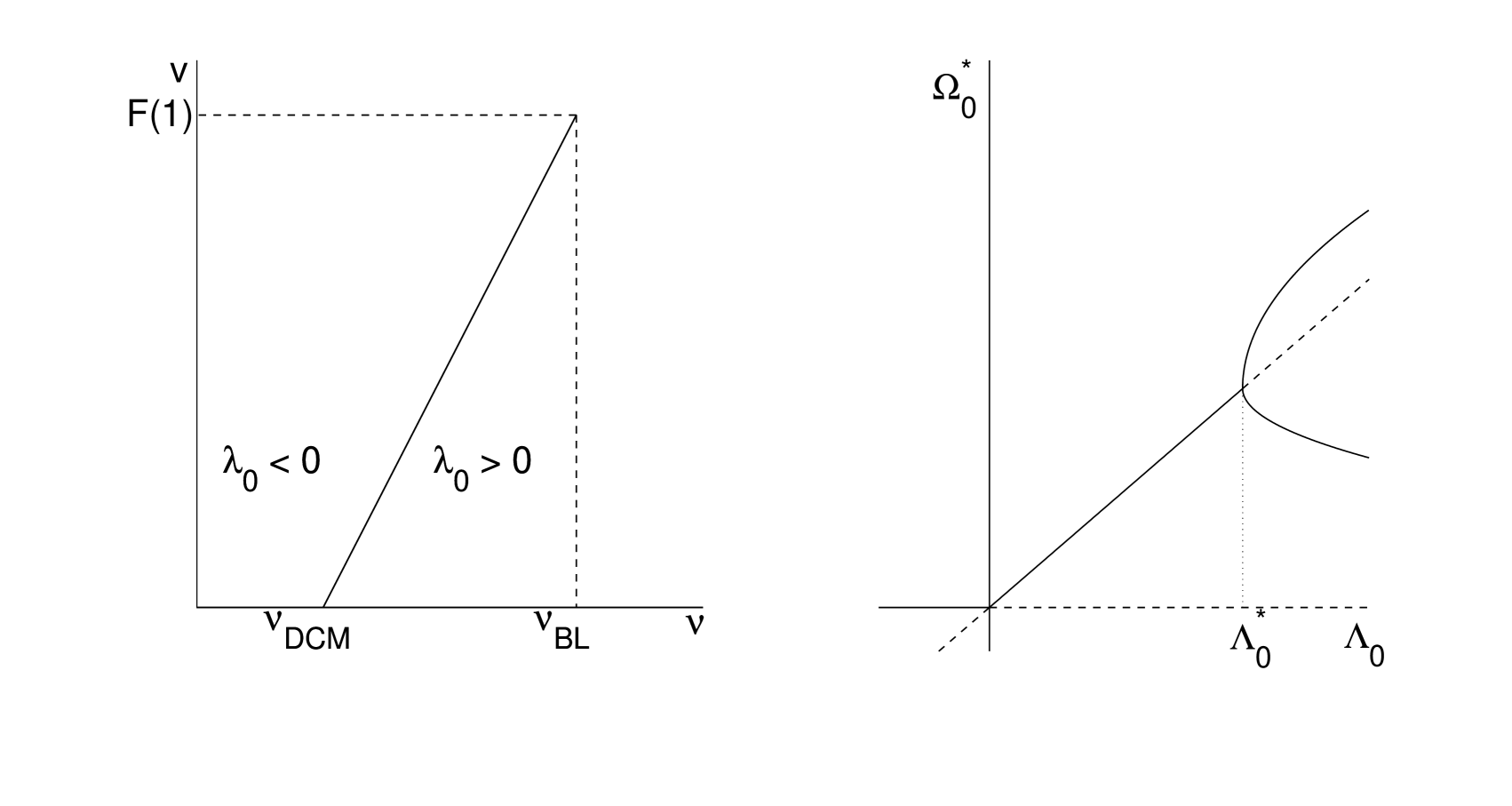
Figure 2: Left panel: the bifurcation diagram for the trivial steady state of (1.5) in the regime $\mathrm{v}<f(0)-f(1)=F(1)$. The trivial steady state is stable in the region $\lambda_{0}<0$ and unstable in the region $\lambda_{0}>0$. Here, $\nu_{DCM}=\ell(1+j_{H})$ and $\nu_{BL}=\ell(1+{\rm e}^{\kappa}j_{H})$. Right panel: the bifurcation diagram for the small-amplitude DCM reported in (1.17) and (1.19). The origin marks the transcritical bifurcation through which the trivial steady state is destabilized and the small-amplitude DCM pattern emerges. The value $\Lambda_{0}^{*}$ marks the (first) Hopf bifurcation where this small-amplitude DCM is destabilized and a time-periodic DCM pattern is generated.

1.2 The asymptotic method

Parallel to understanding the character and fate of the linear destabilization mechanism established in [25], this article has a second—and from a mathematical point of view at least equally important—theme. Here, we have developed a powerful approach by which we can study the weakly nonlinear dynamics generated by (1.5) in full asymptotic detail and far from the region covered by more standard techniques (such as the center manifold reduction method). Indeed, one cannot hope in general to extend the analysis beyond the one-dimensional center manifold reduction discussed above and into the regime where $\lambda_{0}$ is not asymptotically closer to zero than all other eigenvalues. In other words, the sole analytical insight into the dynamics of the flow near the destabilization that one can generically obtain is the confirmation that DCMs indeed appear through a transcritical bifurcation. Let us look into this last point in more detail and for our specific model (1.5)–(1.6). For $\lambda_{0}={\cal O}(\varepsilon)$—equivalently, for $\rho=1$ in (1.16)—one can no longer ‘project away’ the directions corresponding to the eigenvalues $\nu_{n}=-\varepsilon\,(n+1/2)^{2}\,\pi^{2}$ associated with the operator $\mathcal{DT}^{+}$. Indeed, these are ${\cal O}(\varepsilon)$ for ${\cal O}(1)$ values of $n$, and hence of the same asymptotic magnitude as $\lambda_{0}$. As a result, the center manifold reduction approach yields a leading order system in at least asymptotically many dimensions. In general, such a system cannot be studied analytically, and one has to abandon the idea of performing an asymptotically accurate analysis.

The crucial ingredient in our approach is our ability to explicitly determine, to leading order, all relevant coefficients in the reduced, asymptotically high-dimensional system that extends the leading order, one-dimensional center manifold reduction. All of these coefficients are defined in a relatively standard manner in terms of projections based on the linear spectral analysis, see (2.21) in Section 2. We report the outcome of this part of our work in (4.1). These leading order formulas clearly reveal a certain structure in these coefficients, which in turn reflects on the system of ODEs for the Fourier modes. It is this structure that allows us to extend our stability and bifurcation analysis. The sometimes remarkably subtle and laborious analysis by which these coefficients are computed provides the foundation for the strength and success of our program. Therefore, this analysis is a central component of our approach and lies at the core of the forthcoming presentation, see especially Sections 3 and 5–7.

An understanding of the conditions under which similar structure may be expected to appear is apposite to deciphering the fundamental mechanisms underpinning the success of our method and to determining a more general setting where this method is applicable. Naturally, what enables us to compute these coefficients, and thus also determine how they are related, is the accurate asymptotic control over the eigenfunctions that we establish. It is neither clear, a priori, that the structure present in the reduced system is a necessary consequence of that control, nor how much of that control is necessary to establish the presence of sufficient structure. These issues are the subject of current research undertaken by the authors. Below we offer a brief sketch of the ideas behind this work in progress, as it also encapsulates the essentials of the method developed in the present work.

To avoid the computational complexities associated with the weakly nonlinear analysis, we consider a much simpler, autonomous, coupled, reaction–diffusion system,

$$\begin{array}[]{lcrll}U_{t}&=&U_{xx}&+\mu\,U&+F(U,V;\varepsilon),\\ V_{t}&=&\varepsilon\left(V_{xx}\right.&+\nu\,V&+\left.G(U;V,\varepsilon)\right).\end{array}$$ (1.21)

Here, $U$ and $V$ are defined in $[0,1]\times\mathbb{R}^{+}$ and obey certain boundary conditions, e.g., of homogeneous Neumann or Dirichlet type. The nonlinearities $F(U,V)$ and $G(U,V)$ are assumed to be smooth and at least quadratic in $U$ and $V$; finally, $0<\varepsilon\ll 1$ is an asymptotically small parameter. The spectral problem associated with the trivial state $(U,V)\equiv(0,0)$ decouples into two scalar problems of harmonic oscillator type. It immediately follows that, for $\nu$ below a certain critical value $\nu^{*}$, this trivial state loses stability when $\mu$ crosses a threshold $\mu^{*}$. Moreover, the eigenvalues $\{\lambda^{U}_{n}\}_{n\geq 0}$ associated with the $U-$component (and hence also with $\mu$) are ${\cal O}(1)-$apart, while the eigenvalues $\{\lambda^{V}_{n}\}_{n\geq 0}$ associated with the $V-$component (and also with $\nu$) are ${\cal O}(\varepsilon)-$apart. Both sets of eigenvalues are naturally paired with simple trigonometric eigenfunctions. A straightforward center manifold reduction suffices to determine the nature of the bifurcation as $\mu$ crosses $\mu^{*}$ and in the regime $\mu-\mu^{*}\ll\varepsilon$. This situation corresponds directly to our—technically more involved—center manifold problem (1.17)–(1.19) briefly discussed earlier. Note that, here, the leading order analog of the DCM pattern identified in that discussion is a sinusoidal function.

As long as $\mu-\mu^{*}\ll\varepsilon$, the modes associated with the eigenvalues $\{\lambda^{V}_{n}\}_{n}$ remain slaved to the critical $\lambda^{U}_{0}$-mode, exactly as in our phytoplankton–nutrient model. However, this is no longer the case when $\mu-\mu^{*}={\cal O}(\varepsilon)$; in that regime, asymptotically many $\lambda^{v}_{n}$-modes are nonlinearly triggered by that critical mode. Nevertheless, the remaining $\lambda^{U}_{n}$-modes stay slaved, so that one obtains a reduced system of asymptotically high dimension. Here also, the coefficients of the leading nonlinearities can all be expressed in terms of projections along the eigenmodes, albeit they correspond to much simpler integrals. This process should enable us to study the conditions under which one is able to infer relations between these coefficients similar to those reported in (4.1). This, in turn, should lead to conditions under which the reduced system has sufficient structure to allow a secondary bifurcation analysis—and perhaps even the identification of a cascade of subsequent bifurcations—of the nontrivial state bifurcating at $\mu=\mu^{*}$. An additional benefit of working in a simple setting of this sort is its amenability to rigorous analysis, which is beyond the scope of this article.

A natural question to ask at this point is whether the model problem (1.21) shares enough structure with (1.5) to enjoy similarly complex yet tractable dynamics. Note, in particular, the absence of nonlocal and non-autonomous terms from (1.21). Mathematically speaking, we expect these aspects to be insignificant for the type of dynamics that the model exhibits close to bifurcation. (The situation is very different from the ecological point of view, naturally.) In the setting of (1.5), the nonlocality only complicates our analysis and thus clouds our understanding of the secondary and subsequent bifurcations beyond the center manifold reduction. Indeed, one expects the self-shading effect that a small DCM pattern has on itself to be much smaller than the shading due to the water column above it. This is most evident in Sections 3 and 6, where self-shading (quantified by the parameter $r$) is finally shown to contribute higher order terms only. Similarly, the sole role of the non-autonomous features of (1.1) is seemingly to introduce two spectra, $\{\nu_{n}\}_{n}$ and $\{\lambda_{n}\}_{n}$, with different asymptotic properties. In our model problem (1.21), this is achieved instead by choosing disparate diffusivities for the two model components.

Finally, it should be noted that our work resembles, but is certainly not identical to, Lange’s work in [19, 20]. Lange has devised a powerful asymptotic method applicable to problems with closely spaced branch points which allows one to track the evolution of solution branches well into the regime where center manifold reduction breaks down. In our work also, the spectrum is asymptotically closely spaced, as are also then the branch points. Nevertheless, the differences between our work and the work in [19] are substantial. Most prominently, Lange essentially defines branch points as points in parameter space where the linearization around the steady state admits a zero eigenvalue, see the derivation of [19, (3.10)] in particular. In our work, instead, the secondary bifurcation is induced by the parameter-independent negative spectrum related to pure diffusion and occur before any eigenvalues other than $\lambda_{0}$ have bifurcated. As such, these branch points are not captured by Lange’s method. In fact, this secondary bifurcation—and, we expect, part of the cascade toward chaotic dynamics—occurs in a region of parameter space which is asymptotically small compared to the magnitude of the next critical eigenvalue $\lambda_{1}$. Viewed from this perspective, then, the existence of the rich dynamics reported here for the regime $\lambda_{0}={\cal O}(\varepsilon)$ acts as a paradigmatic manifestation of nonlinear interactions. The linearly stable modes manage to have a decisive impact on the dynamics solely through nonlinear couplings and although a strictly linear point of view dictates that these modes should be utterly irrelevant.

2 Evolution of the Fourier coefficients

Our aim in this section is to write the PDE system (1.10) as an infinite-dimensional system of nonlinear ODEs and subsequently reduce it by relaxing the fast stable directions. To achieve this, we need explicit formulas for the (point) spectrum $\sigma(\mathcal{DT}^{+})$, as well as for the corresponding eigenbasis and its dual. The spectrum and the eigenbasis have been determined in [25]; we summarize the relevant formulas in Section 2.1 below. We then obtain the dual basis in Section 2.2 by solving the eigenproblem for the adjoint operator $(\mathcal{DT}^{+})^{*}$. Finally, in Section 2.3, we derive the desired ODEs for the Fourier coefficients close to the bifurcation point.

2.1 The spectrum and the corresponding eigenbasis of $\mathcal{DT}^{+}$

For completeness, we let $\mathcal{H}_{\omega^{+}}$ and $\mathcal{H}_{\eta}$ be the subspaces of $L^{2}(0,1)$ associated with the boundary conditions (1.6), $\mathcal{H}_{\omega}$ be associated with the boundary conditions

$$(\partial_{x}\omega-\sqrt{\mathrm{v}/\varepsilon}\,\omega)(0)=(\partial_{x}\omega-\sqrt{\mathrm{v}/\varepsilon}\,\omega)(1)=0,$$ (2.1)

and we write $\mathcal{H}_{+}=\mathcal{H}_{\omega^{+}}\times\mathcal{H}_{\eta}$ and $\mathcal{H}=\mathcal{H}_{\omega}\times\mathcal{H}_{\eta}$. Both product spaces can be equipped with the inner product

$$\langle u^{+}_{1},u^{+}_{2}\rangle=\left\langle\left(\begin{array}[]{c}\omega^{+}_{1}\\ \eta_{1}\end{array}\right),\left(\begin{array}[]{c}\omega^{+}_{2}\\ \eta_{2}\end{array}\right)\right\rangle=\int_{0}^{1}\Big{(}\omega^{+}_{1}(x)\,\omega^{+}_{2}(x)+\eta_{1}(x)\,\eta_{2}(x)\Big{)}dx.$$

Subsequently, we define the function $E(x)=\exp(\sqrt{\mathrm{v}/\varepsilon}\,x)$ and the operator $\mathcal{E}:\mathcal{H}\to\mathcal{H}_{+}$ corresponding to an application of the Liouville transform,

$$\mathcal{E}u=\left(\begin{array}[]{c}E\,\omega\\ \eta\end{array}\right)=\left(\begin{array}[]{c}\omega^{+}\\ \eta\end{array}\right)=u^{+}\ \mbox{with inverse}\ u=\left(\begin{array}[]{c}\omega\\ \eta\end{array}\right)=\left(\begin{array}[]{c}\omega^{+}/E\\ \eta\end{array}\right)=\mathcal{E}^{-1}u^{+}.$$ (2.2)

(It is straightforward to check that the boundary conditions (1.6) for $u$ yield the boundary conditions (2.1) for $u^{+}$.) Both $\mathcal{E}$ and $\mathcal{E}^{-1}$ are self-adjoint and bounded and

$$\mathcal{DT}=\mathcal{E}^{-1}\mathcal{DT}^{+}\mathcal{E}=\left(\begin{array}[]{cc}\varepsilon\partial_{xx}+f-\ell-\mathrm{v}&0\\ \varepsilon\ell^{-1}fE&\varepsilon\partial_{xx}\end{array}\right),$$ (2.3)

with $\mathcal{DT}$ densely defined and having self-adjoint diagonal blocks.

As mentioned in the Introduction, the eigenvalues $\nu_{n}$ associated with $\mathcal{DT}^{+}$ correspond to the pure diffusion problem for the nutrient in the absence of plankton. In particular, they are solutions to the eigenvalue problem

$$\varepsilon\partial_{xx}\zeta_{n}=\nu_{n}\zeta_{n},\quad\mbox{with}\quad\partial_{x}\zeta_{n}(0)=\zeta_{n}(1)=0,$$

and may be calculated explicitly,

$$\nu_{n}=-\varepsilon N_{n},\quad\mbox{where}\quad N_{n}=(\pi/2+n\pi)^{2}\quad\mbox{for}\ n\geq 0.$$ (2.4)

The corresponding eigenfunctions have a zero $\omega^{+}-$component, and they are

$$v_{n}=\left(\begin{array}[]{c}0\\ \zeta_{n}\end{array}\right),\quad\mbox{where}\ \zeta_{n}(x)=\sqrt{2}\cos(\sqrt{N_{n}}\,x).$$ (2.5)

These are normalized so that $\left|\left|\zeta_{n}\right|\right|_{2}=1$.

The eigenvalues $\lambda_{n}$, on the other hand, correspond to the eigenvectors

$$w^{+}_{n}=\left(\begin{array}[]{c}\omega^{+}_{n}\\ \eta_{n}\end{array}\right).$$

Here, the functions $\omega^{+}_{n}$ and $\eta_{n}$ are solutions to

$$\begin{array}[]{rcl}\varepsilon\,\partial_{xx}\omega^{+}_{n}-2\sqrt{\varepsilon\mathrm{v}}\,\partial_{x}\omega^{+}_{n}+(f(x)-\ell-\lambda_{n})\,\omega^{+}_{n}&=&0,\\ (\partial_{x}\omega^{+}_{n}-2\sqrt{\mathrm{v}/\varepsilon}\,\omega^{+}_{n})(0)=(\partial_{x}\omega^{+}_{n}-2\sqrt{\mathrm{v}/\varepsilon}\,\omega^{+}_{n})(1)&=&0,\end{array}$$

cf. (1.11), together with the self-adjoint, inhomogeneous, boundary value problem for the component $\eta_{n}$,

$$\varepsilon\,\partial_{xx}\eta_{n}-\lambda_{n}\,\eta_{n}=-\varepsilon\ell^{-1}f\,\omega^{+}_{n},\quad\mbox{where}\ \partial_{x}\eta_{n}(0)=\eta_{n}(1)=0.$$ (2.6)

Equivalently, they are solutions to the self-adjoint, Sturm–Liouville problem

$$\begin{array}[]{rcl}\varepsilon\,\partial_{xx}\omega_{n}+(f(x)-\ell-\mathrm{v}-\lambda_{n})\,\omega_{n}&=&0,\\ (\partial_{x}\omega_{n}-\sqrt{\mathrm{v}/\varepsilon}\,\omega_{n})(0)&=&(\partial_{x}\omega_{n}-\sqrt{\mathrm{v}/\varepsilon}\,\omega_{n})(1)=0,\end{array}$$ (2.7)

cf. (2.2)–(2.3). As already stated, in [25] we derived the asymptotic expressions

$$\lambda_{n}=\lambda_{*}-\varepsilon^{1/3}\sigma_{0}^{2/3}\left|A_{n+1}\right|+\Or(\varepsilon^{1/2}),\quad\mbox{with}\ n\geq 0,$$

cf. (1.13). Here, $\lambda_{*}=f(0)-\ell-\mathrm{v}$, $\sigma_{0}=F^{\prime}(0)=-f^{\prime}(0)$, and $A_{n}<0$ is the $n-$th root of the Airy function ${\rm Ai}$, cf. (1.15). A formula for the $n-$th eigenfunction $\omega_{n}$ can also be derived using the WKB method, cf. [25]. The corresponding eigenfunctions for $\mathcal{DT}^{+}$ are $w_{n}^{+}=(\omega^{+}_{n},\eta_{n})^{\rm T}$, where $\omega^{+}_{n}=E\,\omega_{n}$—cf. (2.2). As we will see in the next section, it is natural to impose the normalization condition $\left|\left|\omega_{n}\right|\right|_{2}=1$.

2.2 The dual eigenbasis of $\mathcal{DT}^{+}$

To carry out the weakly nonlinear stability analysis of the bifurcating DCM profile, we also need to obtain the dual eigenbasis $\{\hat{w}^{+}_{n}\}_{n\geq 0}\cup\{\hat{v}_{n}\}_{n\geq 0}$ uniquely determined by the conditions

$$\langle w^{+}_{n},\hat{w}^{+}_{m}\rangle=\langle v_{n},\hat{v}_{m}\rangle=\delta_{nm}\quad\mbox{and}\quad\langle w^{+}_{n},\hat{v}_{m}\rangle=\langle v_{n},\hat{w}^{+}_{m}\rangle=0,$$

for all $n,m\geq 0$. In this section, we show that

$$\hat{w}^{+}_{n}=\left(\begin{array}[]{c}\omega^{-}_{n}\\ 0\end{array}\right)\quad\mbox{and}\quad\hat{v}_{n}=\left(\begin{array}[]{c}\psi^{-}_{n}\\ \zeta_{n}\end{array}\right).$$ (2.8)

Here, $\omega^{-}_{n}\equiv\omega_{n}/E$, where $\omega_{n}$ solves the eigenvalue problem (2.7) and satisfies the normalization condition $\left|\left|\omega_{n}\right|\right|_{2}=1$. Further, expressions for the functions $\{\zeta_{n}\}_{n}$ were reported in (2.5), while the functions $\{\psi^{-}_{n}\}_{n}$ may be found by solving the inhomogeneous problem

$$\begin{array}[]{rcl}\varepsilon\,\partial_{xx}\psi^{-}_{n}+2\sqrt{\varepsilon\mathrm{v}}\,\partial_{x}\psi^{-}_{n}+(f(x)-\ell-\nu_{n})\,\psi^{-}_{n}&=&-\varepsilon\ell^{-1}f\,\zeta_{n},\\ \partial_{x}\psi^{-}_{n}(0)=\partial_{x}\psi^{-}_{n}(1)&=&0.\end{array}$$ (2.9)

Alternatively, $\psi^{-}_{n}=\psi_{n}/E$, where $\psi_{n}$ solves the self-adjoint inhomogeneous problem

$$\begin{array}[]{rcl}\varepsilon\,\partial_{xx}\psi_{n}+(f(x)-\ell-\mathrm{v}-\nu_{n})\,\psi_{n}&=&-\varepsilon\ell^{-1}fE\,\zeta_{n},\\ (\partial_{x}\psi_{n}-\sqrt{\mathrm{v}/\varepsilon}\,\psi_{n})(0)&=&(\partial_{x}\psi_{n}-\sqrt{\mathrm{v}/\varepsilon}\,\psi_{n})(1)=0.\end{array}$$ (2.10)

To verify the above, we start from the observation that the dual basis may be obtained by solving the corresponding eigenvalue problem for $(\mathcal{DT}^{+})^{*}$, the adjoint of the operator $\mathcal{DT}^{+}$. To calculate $(\mathcal{DT}^{+})^{*}$, we write $v^{-}=\mathcal{E}^{-1}v$, recall (2.3), and note that

$$\langle\mathcal{DT}^{+}u^{+},v^{-}\rangle=\langle\mathcal{DT}^{+}\mathcal{E}u,v^{-}\rangle=\langle\mathcal{E}\mathcal{DT}u,v^{-}\rangle=\langle\mathcal{DT}u,\mathcal{E}v^{-}\rangle=\langle\mathcal{DT}u,v\rangle=\langle u,\mathcal{DT}^{*}v\rangle.$$

This implies, further, that

$$\langle\mathcal{DT}^{+}u^{+},v^{-}\rangle=\langle u,\mathcal{DT}^{*}v\rangle=\langle\mathcal{E}^{-1}\,u^{+},\mathcal{DT}^{*}\mathcal{E}v^{-}\rangle=\langle u^{+},\mathcal{E}^{-1}\mathcal{DT}^{*}\mathcal{E}v^{-}\rangle,$$

whence $(\mathcal{DT}^{+})^{*}=\mathcal{E}^{-1}\mathcal{DT}^{*}\mathcal{E}$. Here, $u^{+}$ satisfies the boundary conditions (1.6), whereas the boundary conditions for $v^{-}$ are determined from $v^{-}=\mathcal{E}^{-1}v$ and the boundary conditions (2.1) for $v$—in particular,

$$\partial_{x}\psi^{-}(0)=\partial_{x}\psi^{-}(1)=0\quad\mbox{and}\quad\partial_{x}\zeta(0)=\zeta(1)=0,\quad\mbox{where}\ v=\left(\begin{array}[]{c}\psi^{-}\\ \zeta\end{array}\right).$$ (2.11)

It is straightforward to show that

$$\mathcal{DT}^{*}=\left(\begin{array}[]{cc}\varepsilon\partial_{xx}+f-\ell-\mathrm{v}&\varepsilon\ell^{-1}fE\\ 0&\varepsilon\partial_{xx}\end{array}\right),$$

and, since also $(\mathcal{DT}^{+})^{*}=\mathcal{E}^{-1}\mathcal{DT}^{*}\mathcal{E}$,

$$(\mathcal{DT}^{+})^{*}=\left(\begin{array}[]{cc}\varepsilon\,\partial_{xx}+2\sqrt{\varepsilon\mathrm{v}}\,\partial_{x}+f-\ell&\varepsilon\ell^{-1}f\\ 0&\varepsilon\,\partial_{xx}\end{array}\right).$$ (2.12)

In view of (2.12), the eigenvalue problem $(\mathcal{DT}^{+})^{*}\hat{w}^{+}_{n}=\lambda_{n}\hat{w}^{+}_{n}$ for $\hat{w}^{+}_{n}=({\hat{\omega}^{+}}_{n},{\hat{\eta}}_{n})^{\rm T}$ reads

$$\varepsilon\,\partial_{xx}{\hat{\omega}^{+}}_{n}+2\sqrt{\varepsilon\mathrm{v}}\,\partial_{x}{\hat{\omega}^{+}}_{n}+(f-\ell-\lambda_{n})\,{\hat{\omega}^{+}}_{n}=-\varepsilon\ell^{-1}f\,{\hat{\eta}}_{n},$$

$$\varepsilon\partial_{xx}{\hat{\eta}}_{n}=\lambda_{n}\,{\hat{\eta}}_{n},$$

subject to the boundary conditions (2.11). The latter equation yields immediately ${\hat{\eta}}_{n}\equiv 0$, so that the former equation becomes homogeneous. It is now trivial to check that ${\hat{\omega}^{+}}_{n}=\omega^{-}_{n}\equiv\omega_{n}/E$, where $\omega_{n}$ solves the eigenvalue problem (2.7). This establishes the first part of (2.8).

Similarly, (2.12) shows that the eigenvalue problem $(\mathcal{DT}^{+})^{*}\hat{v}_{n}=\nu_{n}\hat{v}_{n}$ has solutions

$$\hat{v}_{n}=\left(\begin{array}[]{c}\psi^{-}_{n}\\ \zeta_{n}\end{array}\right),$$

where the functions $\{\psi^{-}_{n}\}_{n}$ satisfy the boundary value problem (2.9). An application of the Liouville transform $\psi_{n}=E\psi^{-}_{n}$ leads directly to the self-adjoint problem (2.10).

2.3 Evolution of the Fourier coefficients

Our aim in this section is to write the PDE system (1.10) as an infinite-dimensional system of nonlinear ODEs. We start by expanding the solution of $\partial_{\tau}u^{+}=\mathcal{T}^{+}(u^{+})$ in terms of the eigenbasis associated with the linear stability problem,

$$u^{+}(x,\tau)=\varepsilon^{c-1/6}\,\delta\sum_{n\geq 0}\Omega_{n}(\tau)\,w^{+}_{n}(x)+\varepsilon^{c}\sum_{n\geq 0}\Psi_{n}(\tau)\,v_{n}(x),$$ (2.13)

where $c>0$ is yet undetermined and the coefficients $\Omega_{n}$ and $\Psi_{n}$ are determined by

$$\Omega_{n}=\varepsilon^{-c}\,\delta^{-1}\langle u^{+},\hat{w}^{+}_{n}\rangle\quad\mbox{and}\quad\Psi_{n}=\varepsilon^{-c}\langle u^{+},\hat{v}_{n}\rangle.$$ (2.14)

The exponent of $1/6$ in the first sum of (2.13) is related to the localized nature of $\omega^{+}_{0}$, the planktonic component of $w^{+}_{0}$. In particular, $\omega^{+}_{0}$ is shaped as a DCM with an $\Or(\varepsilon^{1/6})$ biomass $\left|\left|\omega^{+}_{0}\right|\right|_{1}$ (recall from our discussion following (2.8) that, in contrast, $\left|\left|\omega_{0}\right|\right|_{2}=1$). More details on this issue will be presented in Section 4.3.2. Moreover, we have introduced the exponentially small parameter

$$\delta=\exp\left(\frac{-J_{-}({x_{*}})}{\sqrt{\varepsilon}}\right)\ll 1,$$ (2.15)

the role of which is to counterbalance the exponentially large amplitudes of the eigenfunctions $w^{+}_{n}$ and $v_{n}$. In particular,

$$J_{\pm}(x)=\sqrt{\mathrm{v}}\,x\pm I(x)\quad\mbox{and}\quad I(x)=\int_{x_{0}}^{x}\sqrt{F(s)-F(x_{0})}\,ds.$$ (2.16)

Here, the $\Or(\varepsilon^{1/3})-$parameter $x_{0}$ corresponds to the turning point of (2.7),

$$x_{0}=F^{-1}(\lambda_{*}-\lambda_{0})=\varepsilon^{1/3}\sigma_{0}^{-1/3}\left|A_{1}\right|+\Or(\varepsilon^{1/2}),$$ (2.17)

while ${x_{*}}$ is the location of the DCM, the unique point where $J_{-}(\cdot)$ attains its (positive) maximum ([25]—see also A), i.e.,

$${x_{*}}=F^{-1}(\mathrm{v}+F(x_{0}))=F^{-1}(\mathrm{v})+\Or(\varepsilon^{1/3}).$$ (2.18)

Thus, $\delta^{-1}$ is a measure for the amplitude of the $\omega$-component of the (linear) mode associated with a bifurcating DCM. The introduction of $\delta$ in the decomposition (2.13) allows us to identify small patterns ($u^{+}\ll 1$) and is motivated by the observation that this decomposition yields

$$\begin{array}[]{rcl}\omega^{+}(x,\tau)&=&\varepsilon^{c-1/6}\,\delta\sum_{n\geq 0}\Omega_{n}(\tau)\,\omega^{+}_{n}(x),\\ \eta(x,\tau)&=&\varepsilon^{c-1/6}\,\delta\sum_{n\geq 0}\Omega_{n}(\tau)\,\eta_{n}(x)+\varepsilon^{c}\sum_{n\geq 0}\Psi_{n}(\tau)\,\zeta_{n}(x).\end{array}$$ (2.19)

The principal part of $\omega^{+}_{0}$ is derived in A, while asymptotic formulas for $\omega^{+}_{n}$, with $n\geq 1$, can be derived in a similar manner. For $\Or(1)$ values of $n$, it follows that $\omega^{+}_{n}$ is exponentially small everywhere apart from an asymptotically small neighborhood of ${x_{*}}$ where it attains its maximum value of asymptotic magnitude at most $\Or(\varepsilon^{-1/12}\delta^{-1})$. Similarly, the principal part of $\eta_{0}$ is given in B, together with an ${\rm L}^{\infty}-$estimate which shows that $\eta_{0}$ is at most $\Or(\varepsilon^{1/6}\delta^{-1})$ in $[0,1]$. As a result, the coefficients of the eigenmodes $\Omega_{n}$ ($n\geq 0$) in (2.13) are bounded uniformly in $L^{\infty}(0,1)$ by an $\Or(\varepsilon^{c-1/12})$ constant, while those of $\Psi_{n}$ ($n\geq 0$) are $\Or(1)$. In what follows, we derive the ODEs governing the evolution of these eigenmodes.

2.3.1 Eigenbasis decomposition of $\mathcal{T}^{+}(u^{+})$

To derive the ODEs for the eigenmodes, we need to express $\mathcal{T}^{+}(u^{+})$ in the eigenbasis $\{w^{+}_{n}\}_{n\geq 0}\cup\{v_{n}\}_{n\geq 0}$. In particular, we show that

$$\mathcal{T}^{+}(u^{+}) = \varepsilon^{c-1/6}\,\delta\sum_{k\geq 0}\left[\lambda_{k}\,\Omega_{k}-\varepsilon^{c}\,\sum_{m\geq 0}\sum_{n\geq 0}\left(a_{mnk}\,\Omega_{m}\Omega_{n}+b_{mnk}\,\Psi_{m}\Omega_{n}\right)\right]w^{+}_{k}$$ (2.20)

$$+\varepsilon^{c}\sum_{k\geq 0}\left[\nu_{k}\Psi_{k}-\varepsilon^{c}\,\sum_{m\geq 0}\sum_{n\geq 0}\left(a^{\prime}_{mnk}\,\Omega_{m}\Omega_{n}+b^{\prime}_{mnk}\,\Psi_{m}\Omega_{n}\right)\right]v_{k},\hskip 28.45274pt$$

where we have omitted an $\Or(\varepsilon^{3c-1/2})$ remainder. The coefficients appearing in this equation are given by the formulas

$$\begin{array}[]{rcrclcl}a_{mnk}&=&\varepsilon^{-1/6}\left\langle\left(\begin{array}[]{c}1\\ \varepsilon\ell^{-1}\end{array}\right)a_{m}\,\omega^{+}_{n},\hat{w}^{+}_{k}\right\rangle&=&\varepsilon^{-1/6}\langle a_{m}\omega_{n},\omega_{k}\rangle,\vspace*{1mm}\\ a^{\prime}_{mnk}&=&\varepsilon^{-1/3}\left\langle\left(\begin{array}[]{c}1\\ \varepsilon\ell^{-1}\end{array}\right)\delta\,a_{m}\,\omega^{+}_{n},\hat{v}_{k}\right\rangle&=&\varepsilon^{-1/3}\delta\Big{[}\langle a_{m}\omega_{n},\psi_{k}\rangle+\varepsilon\ell^{-1}\langle a_{m}\omega^{+}_{n},\zeta_{k}\rangle\Big{]},\vspace*{1mm}\\ b_{mnk}&=&\left\langle\left(\begin{array}[]{c}1\\ \varepsilon\ell^{-1}\end{array}\right)b_{m}\,\omega^{+}_{n},\hat{w}^{+}_{k}\right\rangle&=&\langle b_{m}\omega_{n},\omega_{k}\rangle,\vspace*{1mm}\\ b^{\prime}_{mnk}&=&\varepsilon^{-1/6}\left\langle\left(\begin{array}[]{c}1\\ \varepsilon\ell^{-1}\end{array}\right)\delta\,b_{m}\,\omega^{+}_{n},\hat{v}_{k}\right\rangle&=&\varepsilon^{-1/6}\delta\Big{[}\langle b_{m}\omega_{n},\psi_{k}\rangle+\varepsilon\ell^{-1}\langle b_{m}\omega^{+}_{n},\zeta_{k}\rangle\Big{]}.\end{array}$$ (2.21)

Here, we have defined the functions

$$\begin{array}[]{rcl}a_{m}&=&\delta\,\left[(1-\nu)\,\eta_{m}+(1-\nu^{-1}f)\,r\,s_{m}\right]f,\quad\mbox{with}\ s_{n}(x)=\int_{0}^{x}\omega^{+}_{n}(s)ds,\\ b_{m}&=&(1-\nu)\,f\,\zeta_{m}.\end{array}$$ (2.22)

Note that we use $\langle\cdot,\cdot\rangle$ to denote all inner products—in $\mathcal{H}$, $\mathcal{H}_{\omega^{+}}$, and ${\mathcal{H}}_{\eta}$—as there is no danger of confusion.

We start by decomposing $\mathcal{T}^{+}(u^{+})$ into linear and nonlinear terms by means of

$$\mathcal{T}^{+}(u^{+})=\mathcal{DT}^{+}u^{+}+\mathcal{N}(u^{+}),\quad\mbox{where}\ \mathcal{N}(u^{+})=\left(\begin{array}[]{c}1\\ \varepsilon\ell^{-1}\end{array}\right)\left(p-f\right)\omega^{+}.$$ (2.23)

Substitution of the decomposition (2.13) into the linear term yields the eigendecomposition of that linear term,

$$\mathcal{DT}^{+}u^{+} = \varepsilon^{c-1/6}\,\delta\sum_{k\geq 0}\Omega_{k}\,\mathcal{DT}^{+}\,w^{+}_{k}+\varepsilon^{c}\sum_{k\geq 0}\Psi_{k}\,\mathcal{DT}^{+}\,v_{k}$$ (2.24)

$$= \varepsilon^{c-1/6}\,\delta\sum_{k\geq 0}\lambda_{k}\,\Omega_{k}w^{+}_{k}+\varepsilon^{c}\sum_{k\geq 0}\nu_{k}\Psi_{k}v_{k},$$

where we have also used that $w^{+}_{n}$ and $v_{n}$ are eigenvectors of $\mathcal{DT}^{+}$ (see Section 2.1). It remains to express the nonlinearity $\mathcal{N}(u^{+})$ with respect to that same eigenbasis. First, since $p-f$ contains the nonlocal term $\int_{0}^{x}\omega^{+}(s)ds$, see (1.7)–(1.8), we write (cf. (2.19))

$$S(x,\tau):=\varepsilon^{-c+1/6}\int_{0}^{x}\omega^{+}(s,\tau)ds=\delta\sum_{n\geq 0}\Omega_{n}(\tau)\,s_{n}(x),$$ (2.25)

where $s_{n}$ was introduced in (2.22). We subsequently obtain, by (1.7) and (1.12),

$$p = \frac{1-\eta}{\nu^{-1}-\eta}\,\frac{1}{1+j_{H}\exp(\kappa x)\exp(\varepsilon^{c-1/6}\,r\,S)}$$

$$= f\,\frac{1-\eta}{1-\nu\eta}\,\frac{1}{1+(1-\nu^{-1}f)(\exp(\varepsilon^{c-1/6}\,r\,S)-1)}.$$

Substituting from (2.19) for $\omega^{+}$ and $\eta$ into this formula and expanding asymptotically, we find further

$$p(\omega^{+},\eta,x) = f-\varepsilon^{c-1/6}\sum_{m\geq 0}a_{m}\Omega_{m}-\varepsilon^{c}\sum_{m\geq 0}b_{m}\Psi_{m}+\Or\left(\varepsilon^{2c-1/3}\right),$$ (2.26)

with $a_{m}$ and $b_{m}$ as defined in (2.22). We remark for later use that this asymptotic expansion remains valid for $o(\varepsilon^{1/4-c})$ values of $\Omega_{n}$ ($n\geq 0$) and $o(\varepsilon^{-c})$ values of $\Psi_{n}$ ($n\geq 0$) (see our discussion following (2.19)). Next, (2.19) and (2.26) yield

$$(p-f)\,\omega^{+}=-\varepsilon^{2c-1/3}\,\delta\sum_{m\geq 0}\sum_{n\geq 0}a_{m}\omega^{+}_{n}\,\Omega_{m}\Omega_{n}-\varepsilon^{2c-1/6}\,\delta\sum_{m\geq 0}\sum_{n\geq 0}b_{m}\omega^{+}_{n}\,\Psi_{m}\Omega_{n},$$

where we have again omitted an $\Or(\varepsilon^{3c-1/2})$ remainder. By virtue of (2.23), then,

$$\mathcal{N}(u^{+}) = -\varepsilon^{2c-1/3}\,\delta\sum_{m\geq 0}\sum_{n\geq 0}\left(\begin{array}[]{c}1\\ \varepsilon\ell^{-1}\end{array}\right)a_{m}\omega^{+}_{n}\,\Omega_{m}\Omega_{n}$$

$$-\varepsilon^{2c-1/6}\,\delta\sum_{m\geq 0}\sum_{n\geq 0}\left(\begin{array}[]{c}1\\ \varepsilon\ell^{-1}\end{array}\right)b_{m}\omega^{+}_{n}\,\Psi_{m}\Omega_{n}+\Or\left(\varepsilon^{3c-1/2}\right).$$

We may now decompose the spatial components in these sums with respect to the eigenbasis,

$$\left(\begin{array}[]{c}1\\ \varepsilon\ell^{-1}\end{array}\right)\delta\,a_{m}\,\omega^{+}_{n}=\sum_{k\geq 0}\left(\varepsilon^{1/6}\delta\,a_{mnk}\,w^{+}_{k}+\varepsilon^{1/3}\,a^{\prime}_{mnk}\,v_{k}\right),$$

$$\left(\begin{array}[]{c}1\\ \varepsilon\ell^{-1}\end{array}\right)\delta\,b_{m}\,\omega^{+}_{n}=\sum_{k\geq 0}\left(\delta\,b_{mnk}w^{+}_{k}+\varepsilon^{1/6}\,b^{\prime}_{mnk}v_{k}\right),$$

where the coefficients $a_{mnk}$, $a^{\prime}_{mnk}$, $b_{mnk}$, and $b^{\prime}_{mnk}$ are found by means of (2.21). Using this decomposition, we finally write (omitting throughout an $\Or(\varepsilon^{3c-1/2})$ term)

$$\mathcal{N}(u^{+}) = -\varepsilon^{2c}\sum_{m\geq 0}\sum_{n\geq 0}\sum_{k\geq 0}\left(\varepsilon^{-1/6}\delta\,a_{mnk}\,w^{+}_{k}+a^{\prime}_{mnk}\,v_{k}\right)\Omega_{m}\Omega_{n}$$ (2.31)

$$-\varepsilon^{2c}\sum_{m\geq 0}\sum_{n\geq 0}\sum_{k\geq 0}\left(\varepsilon^{-1/6}\delta\,b_{mnk}\,w^{+}_{k}+b^{\prime}_{mnk}\,v_{k}\right)\Psi_{m}\Omega_{n}$$

$$= -\varepsilon^{2c-1/6}\delta\sum_{m\geq 0}\sum_{n\geq 0}\sum_{k\geq 0}\left(a_{mnk}\Omega_{m}\Omega_{n}+b_{mnk}\Psi_{m}\Omega_{n}\right)w^{+}_{k}$$

$$-\varepsilon^{2c}\sum_{m\geq 0}\sum_{n\geq 0}\sum_{k\geq 0}\left(a^{\prime}_{mnk}\Omega_{m}\Omega_{n}+b^{\prime}_{mnk}\Psi_{m}\Omega_{n}\right)v_{k}.$$

Combining (2.24) and (2.31), then, we arrive at the desired result (2.20).

2.3.2 ODEs near the bifurcation point

We are now in a position to derive the ODEs for the amplitudes $\{\Omega_{n}\}_{n\geq 0}$ and $\{\Psi_{n}\}_{n\geq 0}$. Differentiating both members of (2.13) with respect to time, we find

$$\partial_{\tau}u^{+}=\varepsilon^{c-1/6}\,\delta\sum_{k\geq 0}\dot{\Omega}_{k}\,w^{+}_{k}+\varepsilon^{c}\sum_{k\geq 0}\dot{\Psi}_{k}\,v_{k},$$ (2.32)

where the overdot denotes differentiation with respect to $\tau$. Next, $\partial_{\tau}u^{+}=\mathcal{T}^{+}(u^{+})$ and hence, combining (2.20) with (2.32), we obtain the ODEs for the amplitudes,

$$\dot{\Omega}_{k} = \lambda_{k}\Omega_{k}-\varepsilon^{c}\,\sum_{m\geq 0}\sum_{n\geq 0}\left(a_{mnk}\,\Omega_{m}\Omega_{n}+b_{mnk}\,\Psi_{m}\Omega_{n}\right)+\Or\left(\varepsilon^{2c}\right),$$

$$\dot{\Psi}_{k} = \nu_{k}\Psi_{k}-\varepsilon^{c}\,\sum_{m\geq 0}\sum_{n\geq 0}\left(a^{\prime}_{mnk}\,\Omega_{m}\Omega_{n}+b^{\prime}_{mnk}\,\Psi_{m}\Omega_{n}\right)+\Or\left(\varepsilon^{2c}\right).$$

We now tune the bifurcation parameter $\lambda_{*}$ so that the largest eigenvalue, $\lambda_{0}$, is the only positive eigenvalue while the eigenvalues $\lambda_{1},\lambda_{2},\ldots$ are negative. In particular, we write (cf. (1.16))

$$\lambda_{0} = \varepsilon\Lambda_{0},\ \mbox{where}\ 0<\Lambda_{0}<<\varepsilon^{-2/3},$$

$$\nu_{k} = -\varepsilon N_{k},\ \mbox{where}\ N_{k}>0\ \mbox{is}\ \Or(1)\ \mbox{for}\ k=0,1,\ldots,$$

$$\lambda_{k} = -\varepsilon^{1/3}\Lambda_{k},\ \mbox{where}\ \Lambda_{k}>0\ \mbox{for}\ k=1,2,\ldots.$$

As we will see shortly, the cases of particular interest will turn out to be those where $\Lambda_{0}$ is either $\Or(1)$ or logarithmically large. Note also that, since the distance between $\lambda_{0}$ and $\lambda_{k}$ is $\Or(\varepsilon^{1/3})$ by (1.13), it follows that $\lambda_{1},\lambda_{2},\ldots\ll\nu_{1}$. Then, the evolution equations for the amplitudes become

$$\dot{\Omega}_{0} =\varepsilon^{\rho}\Lambda_{0}\Omega_{0}-\varepsilon^{c}\sum_{m\geq 0}\sum_{n\geq 0}a_{mn0}\Omega_{m}\Omega_{n}-\varepsilon^{c}\sum_{m\geq 0}\sum_{n\geq 0}b_{mn0}\Psi_{m}\Omega_{n},$$ (2.33)

$$\dot{\Psi}_{k} =-\varepsilon N_{k}\Psi_{k}-\varepsilon^{c}\sum_{m\geq 0}\sum_{n\geq 0}a^{\prime}_{mnk}\Omega_{m}\Omega_{n}-\varepsilon^{c}\sum_{m\geq 0}\sum_{n\geq 0}b^{\prime}_{mnk}\Psi_{m}\Omega_{n},\quad k\geq 0,$$ (2.34)

$$\dot{\Omega}_{k} =-\varepsilon^{1/3}\Lambda_{k}\Omega_{k}-\varepsilon^{c}\sum_{m\geq 0}\sum_{n\geq 0}a_{mnk}\Omega_{m}\Omega_{n}-\varepsilon^{c}\sum_{m\geq 0}\sum_{n\geq 0}b_{mnk}\Psi_{m}\Omega_{n},\quad k\geq 1,$$ (2.35)

where we have omitted all higher order terms.

3 Application of Laplace’s method on $a_{000}$

Explicit asymptotic expressions for the coefficients in the ODEs (2.33)–(2.35) obtained in the previous section can be derived by applying Laplace’s method and the principle of stationary phase to the integrals in (2.21). In this section, we demonstrate the use of the former in deriving an asymptotic formula for $a_{000}$. Asymptotic expressions for the remaining coefficients will be derived independently in Sections 5–7, after we have thoroughly analyzed the bifurcations that our system undergoes. Although the analysis in those sections is substantially more involved, our approach there is very similar to that in the present section.

The main result of this section is the leading order approximation

$$a_{000}=A(\Lambda_{0})=\alpha\,a(\Lambda_{0}),$$ (3.1)

where we have defined the $\Or(1)$, positive, $\Lambda_{0}-$independent constant $\alpha$ and the function $a$ by means of

$$\alpha=(1-\nu)\,f(0)\,C_{1}\,C_{2}\,\sigma_{0}^{1/3}\,\sigma_{*}^{-1/2}>0\quad\mbox{and}\quad a(\Lambda_{0})=\frac{\sinh\left(\sqrt{\Lambda_{0}}(1-{x_{*}})\right)}{\sqrt{\Lambda_{0}}\,\cosh\sqrt{\Lambda_{0}}}.$$ (3.2)

Here, $\sigma_{0}$ is defined in (1.15), while

$$C_{1}=\left(\int_{A_{1}}^{\infty}{\rm Ai}^{2}(s)\,ds\right)^{-1/2},\quad C_{2}=\exp(\left|A_{1}\right|^{3/2}),\quad\mbox{and}\quad\sigma_{*}=F^{\prime}({x_{*}})=-f^{\prime}({x_{*}}),$$ (3.3)

see [25] and A. We start by recalling that the coefficient $a_{000}$ is given by

$$a_{000}=\varepsilon^{-1/6}\,\int_{0}^{1}a_{0}(x)\,\omega^{2}_{0}(x)\,dx,$$ (3.4)

cf. (2.21), where

$$a_{0}(x)=\delta\left[r(1-\nu^{-1}f(x))s_{0}(x)+(1-\nu)\eta_{0}(x)\right]\,f(x).$$

Employing (2.22), (2.25), using the explicit approximation (B.5) for $\eta_{0}$ from B, and defining the functions

$$h_{1}(x,y) = f(x)\,\left[r\,\left(1-\frac{f(x)}{\nu}\right)-\frac{1-\nu}{\ell\sqrt{\Lambda_{0}}}\,\sinh\left(\sqrt{\Lambda_{0}}(x-y)\right)\,f(y)\right],$$ (3.5)

$$h_{2}(x,y) = \frac{(1-\nu)\,f(x)\,\cosh\left(\sqrt{\Lambda_{0}}\,x\right)}{\ell\,\sqrt{\Lambda_{0}}\,\cosh\sqrt{\Lambda_{0}}}\,f(y)\,\sinh\left(\sqrt{\Lambda_{0}}(1-y)\right),$$ (3.6)

we find further

$$a_{0}(x)=\varepsilon^{-1/6}\delta\int_{0}^{x}h_{1}(x,y)\,\omega^{+}_{0}(y)\,dy+\varepsilon^{-1/6}\delta\int_{0}^{1}h_{2}(x,y)\,\omega^{+}_{0}(y)\,dy.$$

Thus,

$$a_{000} =\varepsilon^{-1/6}\delta\int_{0}^{1}\int_{0}^{x}h_{1}(x,y)\,\omega^{2}_{0}(x)\,\omega^{+}_{0}(y)\,dydx+\varepsilon^{-1/6}\delta\int_{0}^{1}\int_{0}^{1}h_{2}(x,y)\,\omega^{2}_{0}(x)\,\omega^{+}_{0}(y)\,dydx$$ (3.7)

$$=\varepsilon^{-1/6}\delta(\mathcal{I}_{1}+\mathcal{I}_{2}),$$

where $\mathcal{I}_{1}$ and $\mathcal{I}_{2}$ are the two double integrals appearing in this expression.

We can obtain the principal parts of $\mathcal{I}_{1}$ and $\mathcal{I}_{2}$ using Theorem D.2, based on [24], in D. We start with the latter integral which, as we will see, fully determines the leading order behavior of $a_{000}$. First, the normalization condition $\|\omega_{0}\|_{2}=1$ yields $\int_{0}^{1}h_{2}(x,y)\,\omega^{2}_{0}(x)\,dx=h_{2}(0,y)$ to leading order. Since, also, $\omega^{+}_{0}$ has a unique maximum at the interior critical point ${x_{*}}$, Theorem D.2.I (with $\lambda=\varepsilon^{-1/2}$, $\Pi=-J_{-}$, and $\Xi=h_{2}(0,\cdot)$) yields

$$\mathcal{I}_{2}=\int_{0}^{1}h_{2}(0,y)\,\omega^{+}_{0}(y)\,dy=\frac{1}{(\varepsilon^{-1/2})^{1/2}}\,\frac{\sqrt{2\pi}\,h_{2}(0,{x_{*}})}{\sqrt{-J_{-}^{\prime\prime}({x_{*}})}}\,\omega^{+}_{0}({x_{*}})=\varepsilon^{1/6}\,\delta^{-1}\,C_{3}$$ (3.8)

to leading order, where we have used the explicit leading order approximation (A.2) of $\omega^{+}_{0}$ from [25] (see also A), recalled the definition (2.15) of $\delta$, defined

$$C_{3}=\frac{\sqrt{2\pi}\,h_{2}(0,{x_{*}})}{\sqrt{-J_{-}^{\prime\prime}({x_{*}})}}\,\frac{C_{1}\,C_{2}\,\sigma_{0}^{1/3}}{2\sqrt{\pi}\,F^{1/4}({x_{*}})}=C_{1}\,C_{2}\,\sigma_{0}^{1/3}\,\sigma_{*}^{-1/2}\,h_{2}(0,{x_{*}}),$$ (3.9)

and employed the identity $J^{\prime\prime}_{-}=-2^{-1}F^{-1/2}F^{\prime}$.

Next, we show $\mathcal{I}_{1}$ to be exponentially smaller than $\mathcal{I}_{2}$. First, we rewrite it as

$$\mathcal{I}_{1}=\varepsilon^{-1/4}\,\frac{C_{1}^{3}\,C_{2}^{3}\,\sigma_{0}}{8\pi^{3/2}}\,\sum_{j=1}^{6}\theta_{j}\int\int_{D}\frac{h_{1}(x,y)}{\sqrt{F(x)}\,F^{1/4}(y)}\,\exp\left(\frac{\Pi_{j}(x,y)}{\sqrt{\varepsilon}}\right)\,dA_{xy},\hskip 21.33955pt$$ (3.10)

where we have used (A.2) and (A.1). Here, $D=\{(x,y)|0\leq y\leq x,\,0\leq x\leq 1\}$ and

$$\begin{array}[]{rclcrcl}\Pi_{1}(x,y)&=&J_{-}(y)-2I(x)&\quad\mbox{and}&\theta_{1}&=&1,\\ \Pi_{2}(x,y)&=&J_{-}(y)-2I(1)&\quad\mbox{and}&\theta_{2}&=&2\theta,\\ \Pi_{3}(x,y)&=&J_{-}(y)+2I(x)-4I(1)&\quad\mbox{and}&\theta_{3}&=&\theta^{2},\\ \Pi_{4}(x,y)&=&J_{+}(y)-2I(x)-2I(1)&\quad\mbox{and}&\theta_{4}&=&\theta,\\ \Pi_{5}(x,y)&=&J_{+}(y)-4I(1)&\quad\mbox{and}&\theta_{5}&=&2\theta^{2},\\ \Pi_{6}(x,y)&=&J_{+}(y)+2I(x)-6I(1)&\quad\mbox{and}&\theta_{6}&=&\theta^{3},\end{array}$$ (3.11)

where $I(x)$ and $J_{\pm 1}(y)$ have been defined in (2.16), and

$$\theta=\frac{\sqrt{\sigma_{1}}+\sqrt{\mathrm{v}}}{\sqrt{\sigma_{1}}-\sqrt{\mathrm{v}}}\quad\mbox{with}\quad\sigma_{1}=F(1).$$ (3.12)

Theorem D.1 yields, for each integral, a result proportional to $\exp(\max_{(x,y)\in D}\Pi_{j}(x,y)/\sqrt{\varepsilon})$. We first identify $\max\Pi_{1}$ and then show that $\max\Pi_{1}>\max\Pi_{j}$, for $j=2,\ldots,6$; it follows that the dominant term in (3.10) corresponds to $\Pi_{1}$ and the rest are exponentially smaller than it. Now, $\Pi_{1}$ has no critical points in $D$, and thus its global maximum lies on

$$\partial D=\bigcup_{i=1}^{3}(\partial D)_{i}=\{(1,y)|0\leq y\leq 1\}\cup\{(x,x)|0\leq x\leq 1\}\cup\{(x,0)|0\leq x\leq 1\}.$$

First, the global maximum cannot be on $(\partial D)_{1}$; indeed, $\mathring{D}$ lies to the left of $(\partial D)_{1}$ and $\partial_{x}\Pi_{1}(x,y)=-2\sqrt{\bar{F}(x)}\leq 0$, where we have introduced $\bar{F}(x)=F(x)-F(x_{0})$, so that $\Pi_{1}$ assumes higher values in $\mathring{D}$ than on $(\partial D)_{1}$. Next, $\Pi_{1}(x,x)=\sqrt{\mathrm{v}}x-3I(x)$ on $(\partial D)_{2}$, and thus $\max\Pi_{1}(x,x)=\Pi_{1}({x^{**}},{x^{**}})$ with $0<{x^{**}}=\bar{F}^{-1}(\mathrm{v}/9)<{x_{*}}$ (recall (2.18) and note that $\bar{F}>0$ is increasing). Finally, $\Pi_{1}(x,0)=-2I(x)\leq 0$ on $(\partial D)_{3}$, and thus $\max_{(\partial D)_{3}}\Pi_{1}\leq 0<\Pi_{1}({x^{**}},{x^{**}})$. In total, then, we find that $\max\Pi_{1}=\Pi_{1}({x^{**}},{x^{**}})>0$. Next, $\Pi_{2}(x,y)\leq\Pi_{1}(x,y)\leq\Pi_{1}({x^{**}},{x^{**}})$. Since the leftmost equality holds only in an $\Or(\varepsilon^{1/2})$-neighborhood of $x=1$, we find that $\max\Pi_{2}<\Pi_{1}({x^{**}},{x^{**}})$, as desired. Additionally, $\Pi_{3}\leq\Pi_{2}$ on $D$, and thus also $\max_{D}\Pi_{3}<\max_{D}\Pi_{1}$. Next, $\Pi_{4}$ has no critical points in $\mathring{D}$, and hence we need to examine its behavior on $\partial D$. First, the maximum cannot be on $(\partial D)_{1}$ by the same argument we used for $\Pi_{1}$. Next, $\Pi_{4}(x,x)=J_{-}(x)-2I(1)$ on $(\partial D)_{2}$, and thus $\max_{(\partial D)_{2}}\Pi_{4}=\Pi_{4}({x_{*}},{x_{*}})=J_{-}({x_{*}})-2I(1)$. Finally, $\Pi_{4}\leq-2I(1)<\Pi_{4}({x_{*}},{x_{*}})$ on $(\partial D)_{3}$, and hence $\max\Pi_{4}=J_{-}({x_{*}})-2I(1)=\max\Pi_{2}<\max\Pi_{1}$, as desired. Finally, $\Pi_{5}\leq\Pi_{4}$ and $\Pi_{6}\leq\Pi_{4}$, and the desired result now follows.

These estimates show, then, that $\max\Pi_{1}=\Pi({x^{**}},{x^{**}})>\max\Pi_{j}$, for $j=2,\ldots,6$. Since $({x^{**}},{x^{**}})\in\partial D$ and its Jacobian satisfies $D\Pi_{1}({x^{**}},{x^{**}})\neq 0$, Theorem D.1 yields for (3.10) the asymptotic formula

$$\mathcal{I}_{1}=\varepsilon^{3/4}\,C^{\prime}_{1}\left(\varepsilon^{-1/4}\,\frac{C_{1}^{3}\,C_{2}^{3}}{8\pi^{3/2}}\,\exp\left(\frac{\Pi_{1}({x^{**}},{x^{**}})}{\sqrt{\varepsilon}}\right)\right)=\varepsilon^{1/2}\,C^{\prime\prime}_{1}\,\exp\left(\frac{\Pi_{1}({x^{**}},{x^{**}})}{\sqrt{\varepsilon}}\right),$$

for some $\Or(1)$ constants $C^{\prime}_{1},C^{\prime\prime}_{1}>0$. Since $\mathcal{I}_{2}={\cal O}(\varepsilon^{1/6}\delta^{-1})$ (3.8) and, by (2.15),

$$\frac{\mathcal{I}_{1}}{\mathcal{I}_{2}}=\varepsilon^{1/3}\frac{C^{\prime\prime}_{1}}{C_{3}}\exp\left(\frac{\Pi_{1}({x^{**}},{x^{**}})-J_{-}({x_{*}})}{\sqrt{\varepsilon}}\right)$$

with

$$\Pi_{1}({x^{**}},{x^{**}})-J_{-}({x_{*}})=[J_{-}({x^{**}})-J_{-}({x_{*}})]-2I({x^{**}})<0$$

(recall that ${x_{*}}$ is defined in (2.18) as the location of the maximum of $J_{-}$), it indeed follows that $\mathcal{I}_{1}$ is exponentially small compared to $\mathcal{I}_{2}$.

We conclude that $a_{000}$ is given by $\delta\,\mathcal{I}_{2}$ at leading order. Combining the expressions (3.8)–(3.9) with the definition of $h_{2}$ in (3.6), we obtain the leading order result (3.1) by using the fact that $f({x_{*}})=\ell$, also at leading order. To derive this last identity, observe that—in the regime $\lambda_{0}\ll 1$—it holds that $\lambda_{*}=0$ at $\Or(1)$, see (1.14), (1.16), or equivalently that $\mathrm{v}=f(0)-\ell$; further, and also to leading order, $F({x_{*}})=\mathrm{v}$ by (2.18), so that the desired identity follows from the definition $F(x)=f(0)-f(x)$ applied at $x={x_{*}}$. Finally, we note that higher order terms in formula (3.1) may be obtained solely by considering $\mathcal{I}_{2}$, as $\mathcal{I}_{1}$ is exponentially smaller than $\mathcal{I}_{2}$.

4 Emergence of a stable DCM

The trivial (zero) state is, by construction, a fixed point of the ODEs (2.33)–(2.35) for the Fourier coefficients. In this and the next section, we identify the remaining fixed points of that system and determine their stability. In this entire section, we work exclusively in the regime $\rho=1$ and $\Lambda_{0}=\Or(1)$.

4.1 Asymptotic expressions for $b_{m00}$, $a^{\prime}_{00k}$, and $b^{\prime}_{m0k}$

As stated in the previous section, where we derived an asymptotic expression for $a_{000}$, asymptotic expressions for the coefficients $b_{m00}$, $a^{\prime}_{00k}$, and $b^{\prime}_{m0k}$ appearing in (2.33)–(2.35) are derived independently in Sections 5–7 below. Here, we summarize the leading order behavior of these coefficients, including also (3.1) for completeness:

$$\begin{array}[]{cclr}a_{000}&=&A(\Lambda_{0}),&{}\hfil\\ b_{m00}&=&B,&\ \mbox{for}\ m\ll\varepsilon^{-1/3},\\ a^{\prime}_{00k}&=&-A^{\prime}_{k}(\Lambda_{0})\,A(\Lambda_{0}),&\ \mbox{for}\ 0\neq k\ll\varepsilon^{-1/3},\\ b^{\prime}_{m0k}&=&-A^{\prime}_{k}(\Lambda_{0})\,B,&\ \mbox{for}\ 0\neq k,m\ll\varepsilon^{-1/3}.\end{array}$$ (4.1)

The function $A$ was introduced in (3.1)–(3.2), whereas $B=\sqrt{2}\,(1-\nu)\,f(0)$ is a positive $\Or(1)$ constant. Further, we have introduced the function $A^{\prime}_{k}$ via

$$A^{\prime}_{k}(\Lambda_{0})=\alpha^{\prime}\,a^{\prime}_{k}(\Lambda_{0}),\quad\mbox{where}\quad\alpha^{\prime}=\frac{\sqrt{2}\,C_{2}\,\sigma_{0}^{1/3}}{C_{1}\,C_{3}\,\sigma_{*}^{1/2}}\quad\mbox{and}\quad a^{\prime}_{k}(\Lambda_{0})=\frac{\cos(\sqrt{N_{k}}\,{x_{*}})}{N_{k}+\Lambda_{0}}.$$ (4.2)

Here, $C_{3}=({\rm Ai}^{\prime}(A_{1}))^{2}$. Note that, similarly to $\alpha$ (cf. (3.2)), $\alpha^{\prime}$ is an $\Or(1)$ constant independent of $\Lambda_{0}$; the constants $\sigma_{0}$, $\sigma_{*}$, $C_{1}$ and $C_{2}$ have been defined in (1.15) and (3.3). We also note the following identity concerning Airy functions (see [5, Section 9.11(iv), identity (9.11.5)])

$$\int_{A_{1}}^{\infty}{\rm Ai}^{2}(s)\,ds=({\rm Ai}^{\prime}(A_{1}))^{2},\quad\mbox{or equivalently}\quad C_{1}^{2}\,C_{3}=1,$$

which, in turn, yields an identity that will prove to be of exceeding importance in the rest of this section—namely,

$$2\alpha=\alpha^{\prime}B.$$ (4.3)

Asymptotic formulas for $b_{m00}$, $a^{\prime}_{00k}$, and $b^{\prime}_{m0k}$ and for higher values of $m$ and $k$ can be derived similarly. However, seeing as such formulas only contribute higher order terms in our analysis below, we refrain from presenting the details. In what follows, instead, we treat (4.1) as being valid for all values of $k$ and $m$.

4.2 The reduced system

The system (2.33)–(2.35) exhibits asymptotically disparate timescales depending on the value of $\rho$ and associated with the asymptotic magnitudes of the eigenvalues. In this section, we investigate the case $\rho=1$, in which regime $\Omega_{0}$ and $\Psi_{0}$, $\Psi_{1}$, $\ldots$ evolve on a slow timescale and the higher-order modes $\Omega_{1}$, $\Omega_{2}$, $\ldots$ become slaved to them. Setting, then, $\rho=1$ and rescaling time (with a slight abuse of notation) as $t=\varepsilon\tau$, the evolution equations become

$$\dot{\Omega}_{0} =\Lambda_{0}\Omega_{0}-\varepsilon^{c-1}\sum_{m\geq 0}\sum_{n\geq 0}a_{mn0}\Omega_{m}\Omega_{n}-\varepsilon^{c-1}\sum_{m\geq 0}\sum_{n\geq 0}b_{mn0}\Psi_{m}\Omega_{n},$$ (4.4)

$$\dot{\Psi}_{k} =-N_{k}\Psi_{k}-\varepsilon^{c-1}\sum_{m\geq 0}\sum_{n\geq 0}a^{\prime}_{mnk}\Omega_{m}\Omega_{n}-\varepsilon^{c-1}\sum_{m\geq 0}\sum_{n\geq 0}b^{\prime}_{mnk}\Psi_{m}\Omega_{n},\quad k\geq 0,$$ (4.5)

$$\varepsilon^{2/3}\dot{\Omega}_{k} =-\Lambda_{k}\Omega_{k}-\varepsilon^{c-1/3}\sum_{m\geq 0}\sum_{n\geq 0}a_{mnk}\Omega_{m}\Omega_{n}-\varepsilon^{c-1/3}\sum_{m\geq 0}\sum_{n\geq 0}b_{mnk}\Psi_{m}\Omega_{n},\quad k\geq 1.$$ (4.6)

(Here also, the overdot denotes differentiation with respect to $t$.) It is natural to introduce slaving relations for the latter modes in this system,

$$\Omega_{k}=\varepsilon^{c_{k}}\,G_{k}(\Omega_{0},\Psi_{1},\Psi_{2},\ldots),\quad\mbox{for all}\quad k\geq 1,$$ (4.7)

where the positive constants $c_{1},c_{2},\ldots$ and the $\Or(1)$ functions (with $\Or(1)$ partial derivatives) $G_{1}$, $G_{2}$, $\ldots$ are to be determined. To do so, we first write the evolution equations for $\Omega_{0}$ and $\Psi_{1}$, $\Psi_{2}$, $\ldots$ under these slaving relations; we find

$$\dot{\Omega}_{0} = \Lambda_{0}\Omega_{0}-\varepsilon^{c-1}a_{000}\Omega_{0}^{2}-\varepsilon^{c-1}\Omega_{0}\sum_{m\geq 0}b_{m00}\Psi_{m},$$

$$\dot{\Psi}_{k} = -N_{k}\Psi_{k}-\varepsilon^{c-1}a^{\prime}_{00k}\Omega_{0}^{2}-\varepsilon^{c-1}\Omega_{0}\sum_{m\geq 0}b^{\prime}_{m0k}\Psi_{m},\quad k\geq 0,$$

where we have retained only the leading order terms from each sum. Dominant balance yields, then, $c=1$. Next, the invariance equation for $\Omega_{k}$ yields that the right member of (4.6) must vanish to leading order. Dominant balance yields $c_{k}=2/3$ and

$$G_{k}(\Omega_{0},\Psi_{1},\Psi_{2},\ldots)=-\frac{a_{00k}}{\Lambda_{k}}\Omega_{0}^{2}-\frac{\Omega_{0}}{\Lambda_{k}}\sum_{m\geq 0}b_{m0k}\Psi_{m}.$$

Recalling, also, (4.1), we arrive at the evolution equations

$$\begin{array}[]{rcrl}\dot{\Omega}_{0}&=&\Lambda_{0}\Omega_{0}-A\,\Omega_{0}^{2}-B\,\Omega_{0}\sum_{m\geq 0}\Psi_{m}\ \ ,&{}\\ \dot{\Psi}_{k}&=&-N_{k}\Psi_{k}+A^{\prime}_{k}\left[A\,\Omega_{0}^{2}+B\,\Omega_{0}\sum_{m\geq 0}\Psi_{m}\right],&k\geq 0.\end{array}$$ (4.8)

Here also, we have retained only the leading order terms from each sum.

Remark 4.1.

The ODE (1.17)—describing the flow on the one-dimensional center manifold in the regime where $\lambda_{0}=\varepsilon^{\rho}\Lambda_{0}\ll\varepsilon$—can be obtained from the system (4.8) above as its $\Lambda_{0}\to 0$ limit. Indeed, the $\Psi$-modes become slaved to the mode $\Omega_{0}$ in this limit, and (4.8) reduces to (1.17) with $a_{000}(0)$ replacing $A=a_{000}(\Lambda_{0})$ (cf. (4.1)). Note that $a_{000}$ has a removable singularity at zero, so we write $a_{000}(0)=\lim_{\Lambda_{0}\to 0}a_{000}(\Lambda_{0})=(1-{x_{*}})\,\alpha$. Using (3.2), it is plain to check that, indeed, the formula for $a_{000}(0)$ reported in (1.19) equals $(1-{x_{*}})\,\alpha$.

4.3 The bifurcating steady state

In this section, we identify the nontrivial fixed point of the reduced system (4.8). In particular, we show that this fixed point is given to leading order by the formulas

$$\Omega_{0}^{*}(\Lambda_{0})=\frac{\Lambda_{0}}{(1-{x_{*}})\,\alpha}\quad\mbox{and}\quad\Psi^{*}_{k}(\Lambda_{0})=\frac{2\,\Lambda_{0}^{2}\,\cos(\sqrt{N_{k}}\,{x_{*}})}{(1-{x_{*}})\,B\,N_{k}\,(N_{k}+\Lambda_{0})},$$ (4.9)

where $k\geq 0$ and the parameter $\alpha$ was introduced in (3.2). Plainly, $\Omega_{0}^{*}$ remains positive, and hence also ecologically relevant, for all positive values of $\Lambda_{0}$ and all values of $0\leq{x_{*}}<1$ (equivalently, all positive values of $\mathrm{v}$ up to the co-dimension two point). Further, the leading order expression (4.9) for $\Omega_{0}^{*}$ exactly matches

$$\Omega_{0}^{*}=\frac{\Lambda_{0}}{a_{000}(0)},\quad\mbox{for}\ \Lambda_{0}\to 0,$$ (4.10)

cf. our discussion in the Introduction and in Remark 4.1 above. It will also be elucidated in Section 4.3.2 below that this fixed point corresponds to a DCM with an $\Or(\varepsilon)$ biomass and an associated $\Or(\varepsilon)$ nutrient depletion.

Note that the denominators in the formulas for $\Omega^{*}_{0}$ and $\Psi^{*}_{k}$ vanish for ${x_{*}}=1$. As explained in the Introduction, this value is attained by ${x_{*}}$ at the co-dimension two point where DCMs and BLs bifurcate concurrently. This is another indication that the nature of the co-dimension two bifurcation is of independent analytical interest.

4.3.1 Derivation of (4.9)

First, setting the left members of (4.8) to zero, we obtain an algebraic system for the nontrivial steady states,

$$\Lambda_{0}-A\,\Omega_{0}-B\sum_{m\geq 0}\Psi_{m}=0,$$ (4.11)

$$N_{k}\Psi_{k}-A^{\prime}_{k}\,\Omega_{0}\,\left[A\,\Omega_{0}+B\sum_{m\geq 0}\Psi_{m}\right]=0.\hskip 28.45274pt$$ (4.12)

Here, $k\geq 0$ and we have removed a superfluous factor of $\Omega_{0}$ in (4.11) corresponding to the trivial steady state. Substituting from this equation into (4.12), we obtain the equivalent formulation

$$A\,\Omega_{0}+B\sum_{m\geq 0}\Psi_{m}=\Lambda_{0}\quad\mbox{and}\quad N_{k}\Psi_{k}-A^{\prime}_{k}\,\Lambda_{0}\,\Omega_{0}=0.$$ (4.13)

This system is readily solved to yield

$$\Omega_{0}^{*}=\frac{\Lambda_{0}}{\alpha^{\prime}\,s\,B\,\Lambda_{0}+A}\quad\mbox{and}\quad\Psi_{k}^{*}=\frac{A^{\prime}_{k}}{N_{k}}\,\Lambda_{0}\,\Omega_{0}^{*},$$ (4.14)

where $s$ is defined by the series

$$s=\frac{1}{\alpha^{\prime}}\sum_{m\geq 0}\frac{A^{\prime}_{m}}{N_{m}}=\sum_{m\geq 0}\frac{\cos(\sqrt{N_{m}}\,{x_{*}})}{N_{m}\,(N_{m}+\Lambda_{0})}.$$

To produce a closed formula for $s$, we recast this formula as

$$s=\sum_{m\geq 0}\frac{\cos(\sqrt{N_{m}}\,{x_{*}})}{N_{m}\,(N_{m}+\Lambda_{0})}=\frac{1}{\Lambda_{0}}\left(\sum_{m\geq 0}\frac{\cos(\sqrt{N_{m}}\,{x_{*}})}{N_{m}}-\sum_{m\geq 0}\frac{\cos(\sqrt{N_{m}}\,{x_{*}})}{N_{m}+\Lambda_{0}}\right),$$ (4.15)

with both series in the right member converging absolutely and uniformly with ${x_{*}}$. The second series appearing in the right member of this last equation is a Mittag-Leffler expansion; analytic formulas for such expansions can often be obtained by means of the Fourier transform. In particular, [21, Eq. (1.63)] (with $a=\pi$, $b={\rm i}\sqrt{\Lambda_{0}}$, and $l=1$) yields the explicit formula

$$\sum_{m\geq 0}\frac{\cos\left(\sqrt{N_{m}}\,{x_{*}}\right)}{N_{m}+\Lambda_{0}}=\frac{\sin\left({\rm i}\sqrt{\Lambda_{0}}\,(1-{x_{*}})\right)}{2{\rm i}\sqrt{\Lambda_{0}}\cos({\rm i}\sqrt{\Lambda_{0}})}=\frac{\sinh\left(\sqrt{\Lambda_{0}}\,(1-{x_{*}})\right)}{2\sqrt{\Lambda_{0}}\cosh\sqrt{\Lambda_{0}}}=\frac{a(\Lambda_{0})}{2},$$ (4.16)

whence also

$$\sum_{m\geq 0}\frac{\cos\left(\sqrt{N_{m}}\,{x_{*}}\right)}{N_{m}}=\frac{a(0)}{2}=\frac{1-{x_{*}}}{2}.$$ (4.17)

Substituting into (4.15), we obtain

$$s=\frac{1-{x_{*}}}{2\Lambda_{0}}-\frac{a(\Lambda_{0})}{2\Lambda_{0}},$$ (4.18)

and therefore (4.14) for $\Omega_{0}^{*}$ becomes

$$\Omega_{0}^{*}=\frac{\Lambda_{0}}{(\alpha-\alpha^{\prime}\,B/2)\,a(\Lambda_{0})+(1-{x_{*}})\,\alpha^{\prime}\,B/2}.$$

The final formulas collected in (4.9) now follow by identity (4.3) and (4.14) for $\Psi_{k}^{*}$.

4.3.2 Ecological interpretation

We next proceed to show that the steady state (stationary pattern) we identified above corresponds to an $\Or(\varepsilon)$ biomass with a corresponding $\Or(\varepsilon)$ depletion of the nutrient. Indeed, (2.19) yields the leading order expression

$$\int_{0}^{1}\omega^{+}(x)\,dx=\varepsilon^{5/6}\,\delta\,\Omega_{0}^{*}\int_{0}^{1}\,\omega^{+}_{0}(x)\,dx$$ (4.19)

for the biomass. Here, we have also recalled that $c=1$ and that $\Omega_{1}^{*},\Omega_{2}^{*},\ldots$ are higher order, cf. (4.7). Recalling the definition of $\delta$ in (2.15) and using the explicit leading order formula (A.2) for $\omega^{+}_{0}$, we obtain

$$\delta\int_{0}^{1}\omega^{+}_{0}(x)\,dx=\varepsilon^{-1/12}\,\frac{C_{1}C_{2}\sigma_{0}^{1/3}}{2\sqrt{\pi}}\int_{0}^{1}F^{-1/4}(x)\exp\left(\frac{J_{-}(x)-J_{-}({x_{*}})}{\sqrt{\varepsilon}}\right)\,dx.$$

As mentioned in Section 3, $J_{-}(\cdot)$ has a sole, locally quadratic maximum at ${x_{*}}$, and hence the integrand above is exponentially small except in an asymptotically small neighborhood of that point. Hence, the integral is of the type considered in D, and Theorem D.1 yields, to leading order,

$$\delta\int_{0}^{1}\omega^{+}_{0}(x)\,dx=\varepsilon^{-1/12}\,\frac{C_{1}\,C_{2}\,\sigma_{0}^{1/3}}{2\sqrt{\pi}}\left(\varepsilon^{1/4}\,\frac{\sqrt{2\pi}}{F^{1/4}({x_{*}})\,\sqrt{-J^{\prime\prime}_{-}({x_{*}})}}\right)=\varepsilon^{1/6}\,C_{1}\,C_{2}\,\sigma_{0}^{1/3}\,\sigma_{*}^{-1/2},$$

where we have also recalled that $J^{\prime\prime}_{-}=-2^{-1}F^{-1/2}F^{\prime}$. Substituting back into (4.19), together with the formula for $\Omega_{0}^{*}$ given in (4.9), we finally recover the first expression (1.20) for the total biomass given in the Introduction. The second expression may be derived by noting that (1.16) implies the leading order result $\nu/(1+j_{H})=\ell+\mathrm{v}$, as well as that $\varepsilon\,\Lambda_{0}=\nu(1+j_{H})^{-1}-\ell-\mathrm{v}$.

Similarly, (2.19) yields the leading order formula

$$\int_{0}^{1}\eta(x)\,dx=\varepsilon^{5/6}\delta\,\Omega^{*}_{0}\,\int_{0}^{1}\eta_{0}(x)\,dx+\varepsilon\sum_{k\geq 0}\Psi^{*}_{k}\int_{0}^{1}\zeta_{k}(x)\,dx.$$ (4.20)

Now, $\int_{0}^{1}\zeta_{k}(x)\,dx=(-1)^{k}/N_{k}$ by (2.5). Further, the integral $\int_{0}^{1}\eta_{0}(x)\,dx$ can be calculated using (B.1): integrating both members over $[0,x]$ and using the boundary condition at zero, we find

$$\ell\,\Lambda_{0}\int_{0}^{1}\eta_{0}(x)\,dx=\ell\,\partial_{x}\eta_{0}(1)+\int_{0}^{1}f(x)\,\omega^{+}_{0}(x)\,dx.$$ (4.21)

The derivative $\partial_{x}\eta_{0}(1)$ can be estimated at leading order by (B.5). Differentiating both members of that formula, we find

$$\ell\,\partial_{x}\eta_{0}(1)=\int_{0}^{1}\left[\tanh\sqrt{\Lambda_{0}}\sinh\left(\sqrt{\Lambda_{0}}(1-y)\right)-\cosh\left(\sqrt{\Lambda_{0}}(1-y)\right)\right]f(y)\,\omega^{+}_{0}(y)\,dy.$$

It follows from (4.21), then, that

$$\ell\,\Lambda_{0}\int_{0}^{1}\eta_{0}(x)\,dx$$

$$\quad=\int_{0}^{1}\left[1+\tanh\sqrt{\Lambda_{0}}\sinh\left(\sqrt{\Lambda_{0}}(1-y)\right)-\cosh\left(\sqrt{\Lambda_{0}}(1-y)\right)\right]\,f(y)\,\omega^{+}_{0}(y)\,dy.$$

Applying Theorem D.1, we obtain

$$\int_{0}^{1}\eta_{0}(x)\,dx=\varepsilon^{1/6}\delta^{-1}\,\frac{C_{1}C_{2}\,\sigma_{0}^{1/3}\,\sigma_{*}^{-1/2}}{\Lambda_{0}}\left(1-\frac{\cosh\left(\sqrt{\Lambda_{0}}\,{x_{*}}\right)}{\cosh\sqrt{\Lambda_{0}}}\right),$$ (4.22)

which is the desired formula for $\int_{0}^{1}\eta_{0}(x)\,dx$. Recalling also (4.9) for $\Psi_{k}^{*}$, we obtain from (4.20) the leading order result

$$\int_{0}^{1}\eta(x)\,dx=\varepsilon\,\Omega_{0}^{*}(\Lambda_{0})\left[\frac{C_{1}C_{2}\,\sigma_{0}^{1/3}\,\sigma_{*}^{-1/2}}{\Lambda_{0}}\left(1-\frac{\cosh\left(\sqrt{\Lambda_{0}}\,{x_{*}}\right)}{\cosh\sqrt{\Lambda_{0}}}\right)+\alpha^{\prime}\,\bar{s}\,\Lambda_{0}\right],$$ (4.23)

where

$$\bar{s}=\frac{1}{\alpha^{\prime}}\sum_{m\geq 0}(-1)^{m}\frac{A^{\prime}_{m}(\Lambda_{0})}{N_{m}^{2}}=\sum_{m\geq 0}(-1)^{m}\frac{\cos\left(\sqrt{N_{m}}\,{x_{*}}\right)}{N_{m}^{2}\,(N_{m}+\Lambda_{0})}=\sum_{m\geq 0}\frac{\sin\left(\sqrt{N_{m}}\,(1-{x_{*}})\right)}{N_{m}^{2}\,(N_{m}+\Lambda_{0})}.$$ (4.24)

This equation, together with (4.9) for $\Omega_{0}^{*}$, yields the total nutrient depletion level to leading order.

4.4 Stability of the small pattern

In this section, we examine the stability of the DCM-like fixed point $(\Omega_{0}^{*},\Psi^{*})=(\Omega_{0}^{*},\Psi_{0}^{*},\Psi_{1}^{*},\ldots)$ which we identified in the previous section. In particular, we show that this fixed point is stabilized through a transcritical bifurcation at $\Lambda_{0}=0$ and that it subsequently undergoes a destabilizing Hopf bifurcation.

4.4.1 The eigenvalue equation

We start by linearizing the ODE system

$$\dot{\Omega}_{0} =\Lambda_{0}\,\Omega_{0}-A\,\Omega_{0}^{2}-B\,\Omega_{0}\sum_{m\geq 0}\Psi_{m},$$

$$\dot{\Psi}_{k} =-N_{k}\Psi_{k}+A^{\prime}_{k}\left[A\,\Omega_{0}^{2}+B\,\Omega_{0}\sum_{m\geq 0}\Psi_{m}\right],\quad\mbox{for all}\ k\geq 0,$$

around $(\Omega_{0}^{*},\Psi^{*})$. Letting $\Omega_{0}=\Omega_{0}^{*}+{{\rm d}\Omega}_{0}$ and $\Psi_{k}=\Psi^{*}_{k}+{{\rm d}\Psi}_{k}$ and recalling (4.13), we find that the corresponding linearized problem reads

$$\dot{{{\rm d}\Omega}}_{0} =-A\,\Omega_{0}^{*}\,{{\rm d}\Omega}_{0}-B\,\Omega_{0}^{*}\sum_{m\geq 0}{{\rm d}\Psi}_{m},$$ (4.25)

$$\dot{{{\rm d}\Psi}}_{k} =A^{\prime}_{k}\,\left[\Lambda_{0}+A\,\Omega_{0}^{*}\right]\,{{\rm d}\Omega}_{0}+\left[A^{\prime}_{k}\,B\,\Omega_{0}^{*}-N_{k}\right]\,{{\rm d}\Psi}_{k}+A^{\prime}_{k}\,B\,\Omega_{0}^{*}\,\sum_{m\neq k}{{\rm d}\Psi}_{m},$$ (4.26)

where we have only retained the leading order component from each term.

Truncating at the arbitrary value $k=K\in\mathbf{N}$, we obtain the system $\dot{\delta\Phi}=\mathcal{L}_{K}\,\delta\Phi$, where $\delta\Phi=({{\rm d}\Omega}_{0},{{\rm d}\Psi}_{0},{{\rm d}\Psi}_{1},\ldots,{{\rm d}\Psi}_{K})^{\rm T}$ and

$$\mathcal{L}_{K}=\left(\begin{array}[]{cccccc}-A\,\Omega_{0}^{*}&-B\,\Omega_{0}^{*}&-B\,\Omega_{0}^{*}&\ldots&-B\,\Omega_{0}^{*}\vspace*{0.25cm}\\ A^{\prime}_{0}(A\,\Omega_{0}^{*}+\Lambda_{0})&A^{\prime}_{0}\,B\,\Omega_{0}^{*}-N_{0}&A^{\prime}_{0}\,B\,\Omega_{0}^{*}&\ldots&A^{\prime}_{0}\,B\,\Omega_{0}^{*}\vspace*{0.25cm}\\ A^{\prime}_{1}(A\,\Omega_{0}^{*}+\Lambda_{0})&A^{\prime}_{1}\,B\,\Omega_{0}^{*}&A^{\prime}_{1}\,B\,\Omega_{0}^{*}-N_{1}&\ldots&A^{\prime}_{1}\,B\,\Omega_{0}^{*}\vspace*{0.25cm}\\ \vdots&\vdots&\vdots&\ddots&\vdots\vspace*{0.25cm}\\ A^{\prime}_{K}(A\,\Omega_{0}^{*}+\Lambda_{0})&A^{\prime}_{K}\,B\,\Omega_{0}^{*}&A^{\prime}_{K}\,B\,\Omega_{0}^{*}&\ldots&A^{\prime}_{K}\,B\,\Omega_{0}^{*}-N_{K}\vspace*{0.25cm}\end{array}\right).$$

To characterize the spectrum of this matrix, we derive a formula for its characteristic polynomial $\det(\mathcal{L}_{0}-\lambda I)$. First, we use the first row of $\mathcal{L}_{0}-\lambda I$ to eliminate the off-diagonal entries of all other rows. In this way, we find that the equation $\det(\mathcal{L}_{0}-\lambda I)=0$ is equivalent to setting to zero the determinant

$$\left|\begin{array}[]{ccccc}\lambda+A\,\Omega_{0}^{*}&B\,\Omega_{0}^{*}&B\,\Omega_{0}^{*}&\ldots&B\,\Omega_{0}^{*}\\ A^{\prime}_{0}(\lambda-\Lambda_{0})&\lambda+N_{0}&0&\ldots&0\vspace*{0.25cm}\\ A^{\prime}_{1}(\lambda-\Lambda_{0})&0&\lambda+N_{1}&\ldots&0\vspace*{0.25cm}\\ \vdots&\vdots&\vdots&\ddots&\vdots\vspace*{0.25cm}\\ A^{\prime}_{K}(\lambda-\Lambda_{0})&0&0&\ldots&\lambda+N_{K}\end{array}\right|.$$

Next, we can use the $(k+2)-$nd column to eliminate the $(k+2)-$nd entry of the first column, for $0\leq k\leq K$, as long as $\lambda\neq-N_{k}$. Since $\lambda=-N_{k}$ if and only if $A^{\prime}_{k}=0$ (as can be shown by expanding the determinant along the $(k+2)-$nd row), we can eliminate all entries of the first column. (Note that $A^{\prime}_{k}$ may indeed be zero: indeed, $A^{\prime}_{k}$ is proportional to $\cos((k+1/2)\pi\,{x_{*}})$, which may or may not be zero depending on the values of $k$ and ${x_{*}}$.) Defining ${\cal K}=\{k:A^{\prime}_{k}\neq 0\}\subset\{0,\ldots,K\}$, ${\cal K}_{k}={\cal K}-\{k\}$, and eliminating the entries of the first column as detailed above, we obtain

$$\left|\begin{array}[]{ccccc}Q(\lambda)&B\,\Omega_{0}^{*}&B\,\Omega_{0}^{*}&\ldots&B\,\Omega_{0}^{*}\vspace*{0.25cm}\\ 0&\lambda+N_{0}&0&\ldots&0\vspace*{0.25cm}\\ 0&0&\lambda+N_{1}&\ldots&0\vspace*{0.25cm}\\ \vdots&\vdots&\vdots&\ddots&\vdots\vspace*{0.25cm}\\ 0&0&0&\ldots&\lambda+N_{K}\end{array}\right|=0.$$ (4.27)

Here,

$$Q(\lambda) =(\lambda+A\,\Omega_{0}^{*})\prod_{k\in{\cal K}}(\lambda+N_{k})+B\,\Omega_{0}^{*}\,(\Lambda_{0}-\lambda)\sum_{k\in{\cal K}}A^{\prime}_{k}\prod_{m\in{\cal K}_{k}}(\lambda+N_{m}).$$

As detailed above, $\lambda=-N_{k}$ solves (4.27) if and only if $A^{\prime}_{k}=0$ (equivalently, if and only if $k\not\in{\cal M}$). Further, $\Lambda_{0}>0$ cannot be an eigenvalue, since $Q(\Lambda_{0})>0$ and $\Lambda_{0}+\mathbf{N}_{k}>0$, for all $k\in\{0,\ldots,K\}$—note that $A,N_{0},N_{1},\ldots,N_{K}$ are all positive constants. Hence, we can extend the set over which we sum in the formula above to the entire set $\{0,\ldots,K\}$ and rewrite the equation for $Q(\lambda)$ in the form

$$Q(\lambda)=\left[B\,\Omega_{0}^{*}\sum_{k=0}^{K}\frac{A^{\prime}_{k}}{N_{k}+\lambda}-\frac{\lambda+A\,\Omega_{0}^{*}}{\lambda-\Lambda_{0}}\right](\Lambda_{0}-\lambda)\prod_{k\in{\cal K}}(N_{k}+\lambda).$$

As we just noted, the elements of the set $\{-N_{k}\}_{k\in\cal K}$ are not eigenvalues of $\mathcal{L}_{0}$. Hence, the eigenvalues of $\mathcal{L}_{0}$ are $\{-N_{k}\}_{k\not\in\cal K}$ together with all solutions to

$$B\,\Omega_{0}^{*}\sum_{k=0}^{K}\frac{A^{\prime}_{k}}{N_{k}+\lambda}=\frac{\lambda+A\,\Omega_{0}^{*}}{\lambda-\Lambda_{0}}.$$

Substituting for $A^{\prime}_{k}$ from (4.2) and for $\Omega_{0}^{*}$ from (4.9), recalling the identity (4.3), and letting $K\to\infty$, we rewrite this equation in the form

$$\frac{2\Lambda_{0}}{1-{x_{*}}}\,\sum_{k\geq 0}\frac{\cos\left(\sqrt{N_{k}}\,{x_{*}}\right)}{(N_{k}+\lambda)\,(N_{k}+\Lambda_{0})}=\frac{\lambda+\Lambda_{0}\,a(\Lambda_{0})/(1-{x_{*}})}{\lambda-\Lambda_{0}}.$$

Here again, we may write

$$\sum_{k\geq 0}\frac{\cos\left(\sqrt{N_{k}}\,{x_{*}}\right)}{(N_{k}+\lambda)\,(N_{k}+\Lambda_{0})} = \frac{1}{\lambda-\Lambda_{0}}\left(\sum_{k\geq 0}\frac{\cos\left(\sqrt{N_{k}}\,{x_{*}}\right)}{N_{k}+\Lambda_{0}}-\sum_{k\geq 0}\frac{\cos\left(\sqrt{N_{k}}\,{x_{*}}\right)}{N_{k}+\lambda}\right)$$

$$= \frac{1}{2}\frac{a(\Lambda_{0})-a(\lambda)}{\lambda-\Lambda_{0}},$$

so that the eigenvalue problem becomes $(1-{x_{*}})\,\lambda+\Lambda_{0}\,a(\lambda)=0$. Recalling that $a(0)=1-{x_{*}}$, we recast this equation as

$$\lambda\,\frac{a(0)}{a(\lambda)}=-\Lambda_{0},\quad\mbox{where we recall that}\ a(\lambda)=\frac{\sinh\left(\sqrt{\lambda}(1-{x_{*}})\right)}{\sqrt{\lambda}\,\cosh\sqrt{\lambda}}.$$ (4.28)

This equation is satisfied by some $\lambda$ if and only if it is also satisfied by its complex conjugate $\lambda^{*}$, as the right member is real and $(\lambda^{-1}a(\lambda))^{*}=(\lambda^{*})^{-1}a(\lambda^{*})$. Hence, we may restrict $\arg(\lambda)$ to lie in $[0,\pi]$. Further writing $\mu:=\sqrt{\lambda}=\mu_{R}+{\rm i}\,\mu_{I}$, we rewrite the eigenvalue equation in its final form,

$$p(\mu):=-\frac{(1-{x_{*}})\,\mu^{3}\,\cosh\mu}{\sinh\left((1-{x_{*}})\,\mu\right)}=\Lambda_{0},\quad\mbox{with}\ \arg(\mu)\in[0,\pi/2].$$ (4.29)

We note here for later use that

$$\frac{{\rm Re}(p(\mu))}{1-{x_{*}}} = \mu_{R}(3\mu_{I}^{2}-\mu_{R}^{2})\frac{\sinh[(2-{x_{*}})\mu_{R}]\cos({x_{*}}\mu_{I})-\sinh({x_{*}}\mu_{R})\cos[(2-{x_{*}})\mu_{I}]}{\cosh[2(1-{x_{*}})\mu_{R}]-\cos[2(1-{x_{*}})\mu_{I}]}$$

$$+\mu_{I}(3\mu_{R}^{2}-\mu_{I}^{2})\frac{\cosh[(2-{x_{*}})\mu_{R}]\sin({x_{*}}\mu_{I})-\cosh({x_{*}}\mu_{R})\sin[(2-{x_{*}})\mu_{I}]}{\cosh[2(1-{x_{*}})\mu_{R}]-\cos[2(1-{x_{*}})\mu_{I}]},$$

$$\frac{{\rm Im}(p(\mu))}{1-{x_{*}}} = \mu_{I}(\mu_{I}^{2}-3\mu_{R}^{2})\frac{\sinh[(2-{x_{*}})\mu_{R}]\cos({x_{*}}\mu_{I})-\sinh({x_{*}}\mu_{R})\cos[(2-{x_{*}})\mu_{I})]}{\cosh[2(1-{x_{*}})\mu_{R}]-\cos[2(1-{x_{*}})\mu_{I}]}$$

$$+\mu_{R}(3\mu_{I}^{2}-\mu_{R}^{2})\frac{\cosh[(2-{x_{*}})\mu_{R}]\sin({x_{*}}\mu_{I})-\cosh({x_{*}}\mu_{R})\sin[(2-{x_{*}})\mu_{I}]}{\cosh[2(1-{x_{*}})\mu_{R}]-\cos[2(1-{x_{*}})\mu_{I}]}.$$

4.4.2 Analysis of (4.29) for $\Lambda_{0}\downarrow 0$

We first establish that, as $\Lambda_{0}\downarrow 0$, the eigenvalues $\{\lambda_{n}\}_{n\geq-1}$ remain each in a neighborhood of the discrete values $-\Lambda_{0},-N_{0},-N_{1},\ldots$.

For $\Lambda_{0}=0$, (4.29) yields either $\mu=0$ (equivalently, $\lambda=0$) or $\cosh\mu=0$ (whence $\mu={\rm i}\,\sqrt{N_{m}}$, $m\geq 0$ or, equivalently, $\lambda\in\{-N_{m}\}_{m\geq 0}$). To investigate the possibility of negative eigenvalues $\lambda$ for $\Lambda_{0}>0$, we set $\mu_{R}=0$ to find that (4.29) reduces to

$$p({\rm i}\mu_{I})=\frac{(1-{x_{*}})\,\mu_{I}^{3}}{1-\cos[2(1-{x_{*}})\mu_{I}]}\sin[(1-{x_{*}})\,\mu_{I}]\,\cos\mu_{I}=\Lambda_{0}.$$ (4.30)

For $\Lambda_{0}\downarrow 0$, there is plainly a small root of this equation, $\mu_{I}=\sqrt{\Lambda_{0}}+\Or(\Lambda_{0})$, yielding the small eigenvalue $\lambda=-\Lambda_{0}+\Or(\Lambda_{0}^{2})$. Additionally, all eigenvalues of the set $\{-N_{m}\}_{m\geq 1}$ perturb and remain real for small enough values of $\Lambda_{0}>0$. Indeed, $p({\rm i}\cdot)$ intersects zero transversally at $\{\sqrt{N_{m}}\}_{m\geq 0}$, whence the persistence of any finite number of eigenvalues from among this set is automatically established. That the remaining, infinitely many eigenvalues also persist can be established by noting that, if the maximum value of $p({\rm i}\cdot)$ is positive between successive zeros, then this value grows unboundedly with $\mu_{I}$. For the two first eigenvalues, in particular, we have the Taylor expansions

$$\lambda_{-1}=-\Lambda_{0}+\Or(\Lambda_{0}^{2})\quad\mbox{and}\quad\lambda_{0}=-N_{0}+4\frac{\sin[(1-{x_{*}})\,\pi/2]}{(1-{x_{*}})\,\pi}\Lambda_{0}+\Or(\Lambda_{0}),$$

which demonstrate that both remain in the interval $(-N_{0},0)$ and approach each other as $\Lambda_{0}$ increases, see also Figure 3. These are precisely the two first eigenvalues that collide as $\Lambda_{0}$ is increased, yielding a pair of complex conjugate eigenvalues.

Next, the possibility of positive eigenvalues $\lambda$—equivalently, positive solutions of (4.29)—can be excluded by noticing that $-\Lambda_{0}<0$ while $p(\mu)>0$ for all $\mu>0$. In fact, the possibility of eigenvalues anywhere but in a neighborhood of the negative axis can be similarly excluded by observing that

$$\left|p(\mu)\right|=(1-{x_{*}})\left|\mu\right|^{3}\left(\frac{\cosh(2\mu_{R})+\cos(2\mu_{I})}{\cosh[2(1-{x_{*}})\mu_{R}]-\cos[2(1-{x_{*}})\mu_{I}]}\right)^{1/2}\to\infty,\quad\mbox{as}\quad\mu_{R}\to\infty.$$

Plainly, for every value of $\Lambda_{0}$, there exists a value $\mu_{R}^{*}(\Lambda_{0})>0$ which depends continuously on $\Lambda_{0}$, satisfies $\lim_{\Lambda_{0}\to 0}\mu_{R}^{*}(\Lambda_{0})=0$, and is such that the equation $\left|p(\mu)\right|=\left|\Lambda_{0}\right|$ cannot be satisfied for any $\mu_{R}>\mu_{R}^{*}(\Lambda_{0})$. It follows that all solutions to (4.29) must lie in the half plane $\{\mu\,|\,\mu_{R}\leq\mu_{R}^{*}(\Lambda_{0})\}$ which, in turn, corresponds to a neighborhood of the half axis $\{\lambda\in\mathbf{R}\,|\,\lambda\leq\left|\mu_{R}^{*}(\Lambda_{0})\right|^{2}\}$. A local analysis around the origin now establishes the absence of eigenvalues with positive real parts, for $\Lambda_{0}$ small enough, and hence also the result.

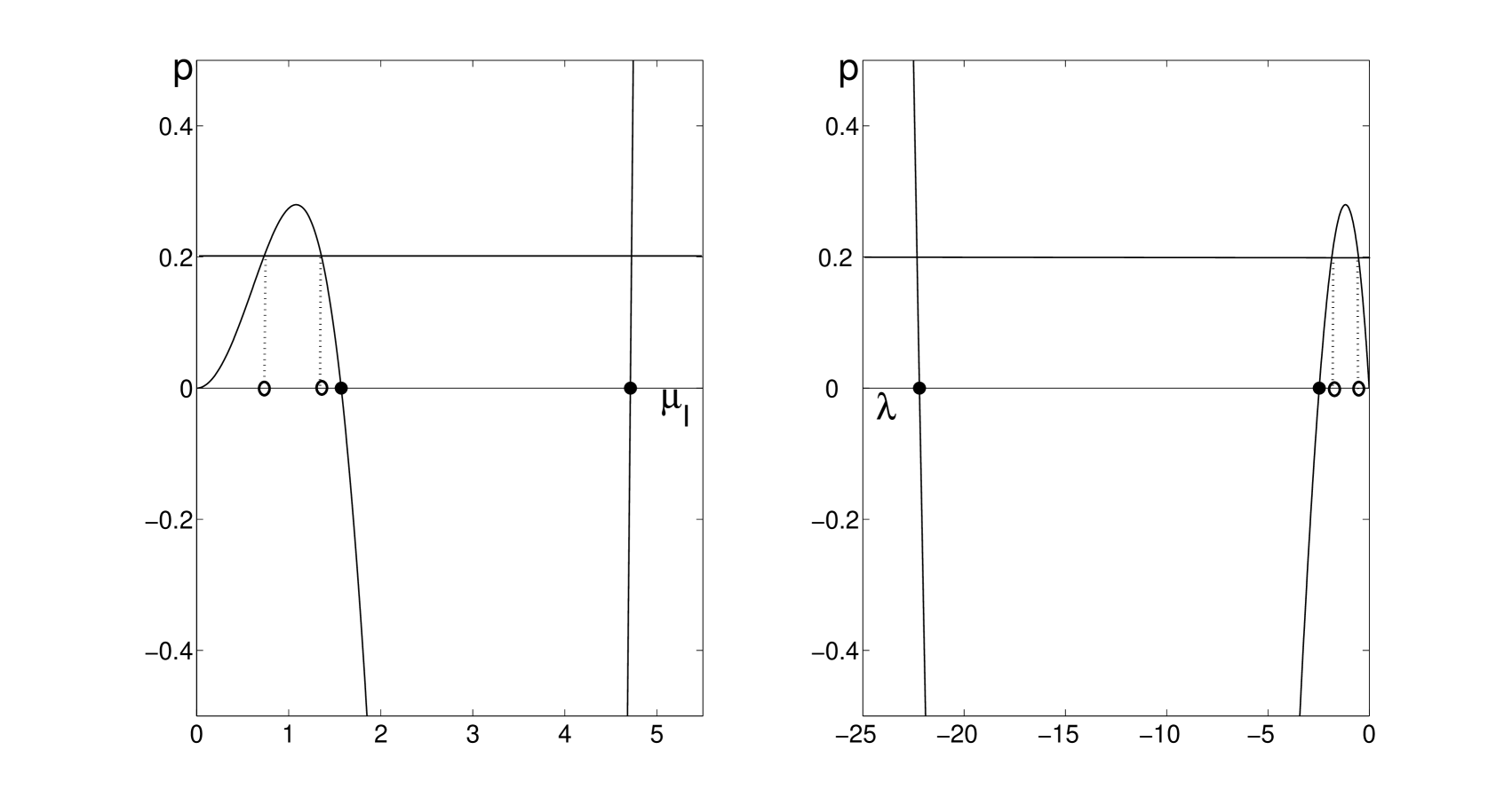
Figure 3: Plots of the function $p({\rm i}\mu_{I})$ (see (4.30)) versus $\mu_{I}$ (left panel) and versus $\lambda=-\mu_{I}^{2}$ (right panel) for ${x_{*}}=0.7$. Also plotted: the level line at $p=\Lambda_{0}$, here set at $0.2$; the first two members of the sequence $\{\sqrt{N}_{k}\}_{k\geq 0}$ (left panel) and $\{-N_{k}\}_{k\geq 0}$ (right panel) as solid dots; and the two smallest solutions $\mu_{I}$ to (4.30) (left panel) together with the first two eigenvalues $\lambda_{-1}$ and $\lambda_{0}$ (right panel) they correspond to, all as hollow dots.

4.4.3 Complexification of eigenvalues and the Hopf bifurcation

As we briefly mentioned in the last section in conjunction with Figure 3, the two principal eigenvalues $\lambda_{-1}$ and $\lambda_{0}$ come closer together as $\Lambda_{0}$ increases. Eventually, they collide at a specific value $\mu_{I}^{\prime}\in(0,\pi/2)$ and for $\Lambda_{0}=\Lambda_{0}^{\prime}=p({\rm i}\mu_{I}^{\prime})=\max_{\mu_{I}\in(0,\pi/2)}p({\rm i}\mu_{I})>0$. For $\Lambda_{0}>\Lambda_{0}^{\prime}$, this pair of eigenvalues becomes complex, so it is natural to examine whether it crosses into the right half-plane through the imaginary axis. (Note that no eigenvalues can cross through zero, as (4.28) does not admit a zero eigenvalue for $\Lambda_{0}>0$.)

To locate imaginary eigenvalues $\lambda={\rm i}\lambda_{I}\in{\rm i}\mathbf{R}$, we set $\mu_{R}=\mu_{I}=\bar{\mu}>0$ and rewrite the real and imaginary parts of $p$ as

$${\rm Re}(p(\mu)) = 2(1-{x_{*}})\bar{\mu}^{3}\left[\frac{\cosh[(2-{x_{*}})\bar{\mu}]\sin({x_{*}}\bar{\mu})-\cosh({x_{*}}\bar{\mu})\sin[(2-{x_{*}})\bar{\mu}]}{\cosh[2(1-{x_{*}})\bar{\mu}]-\cos[2(1-{x_{*}})\bar{\mu}]}\right.$$

$$\left.\hskip 71.13188pt+\frac{\sinh[(2-{x_{*}})\bar{\mu}]\cos({x_{*}}\bar{\mu})-\sinh({x_{*}}\bar{\mu})\cos[(2-{x_{*}})\bar{\mu}]}{\cosh[2(1-{x_{*}})\bar{\mu}]-\cos[2(1-{x_{*}})\bar{\mu}]}\right],$$

$${\rm Im}(p(\mu)) = 2(1-{x_{*}})\bar{\mu}^{3}\left[\frac{\cosh[(2-{x_{*}})\bar{\mu}]\sin({x_{*}}\bar{\mu})-\cosh({x_{*}}\bar{\mu})\sin[(2-{x_{*}})\bar{\mu}]}{\cosh[2(1-{x_{*}})\bar{\mu}]-\cos[2(1-{x_{*}})\bar{\mu}]}\right.$$

$$\left.\hskip 71.13188pt-\frac{\sinh[(2-{x_{*}})\bar{\mu}]\cos({x_{*}}\bar{\mu})-\sinh({x_{*}}\bar{\mu})\cos[(2-{x_{*}})\bar{\mu})]}{\cosh[2(1-{x_{*}})\bar{\mu}]-\cos[2(1-{x_{*}})\bar{\mu}]}\right].$$

The condition ${\rm Im}(p(\mu))=0$, derived from (4.29), yields

$$\cosh[(2-{x_{*}})\bar{\mu}]\sin({x_{*}}\bar{\mu})-\cosh({x_{*}}\bar{\mu})\sin[(2-{x_{*}})\bar{\mu}]$$

$$=\sinh[(2-{x_{*}})\bar{\mu}]\cos({x_{*}}\bar{\mu})-\sinh({x_{*}}\bar{\mu})\cos[(2-{x_{*}})\bar{\mu})].$$ (4.31)

Therefore, the equation ${\rm Re}(p(\mu))=\Lambda_{0}$, similarly derived from (4.29), becomes

$$4(1-{x_{*}})\bar{\mu}^{3}\,\frac{\cosh[(2-{x_{*}})\bar{\mu}]\sin({x_{*}}\bar{\mu})-\cosh({x_{*}}\bar{\mu})\sin[(2-{x_{*}})\bar{\mu}]}{\cosh[2(1-{x_{*}})\bar{\mu}]-\cos[2(1-{x_{*}})\bar{\mu}]}=\Lambda_{0}.$$ (4.32)

Condition (4.31) determines the values of $\bar{\mu}$ corresponding to imaginary eigenvalues $\lambda=2{\rm i}\bar{\mu}^{2}$, while (4.32) yields the corresponding values of $\Lambda_{0}$ for which these eigenvalues appear. Since the former of these can be recast as

$$\mathrm{e}^{(2-{x_{*}})\bar{\mu}}\sin\left({x_{*}}\bar{\mu}-\frac{\pi}{4}\right) - \mathrm{e}^{{x_{*}}\bar{\mu}}\sin\left((2-{x_{*}})\bar{\mu}-\frac{\pi}{4}\right)$$ (4.33)

$$+ \mathrm{e}^{-(2-{x_{*}})\bar{\mu}}\sin\left({x_{*}}\bar{\mu}+\frac{\pi}{4}\right)-\mathrm{e}^{-{x_{*}}\bar{\mu}}\sin\left((2-{x_{*}})\bar{\mu}+\frac{\pi}{4}\right)\!=\!0,\hskip 28.45274pt$$

we see that there exists a whole, discrete sequence $\{\bar{\mu}_{k}\}_{k\geq 0}$ of values $\bar{\mu}$, see also Figure 4. As $k\to\infty$, $\{\bar{\mu}_{k}\}_{k\geq 0}$ limits to $\{(k+1/4)\pi\,{x_{*}}^{-1}\}_{k\geq 0}$, the sequence of the set of zeroes of the first term in (4.33) which becomes dominant in the regime $\bar{\mu}\to\infty$. Equation (4.32) yields the leading order result

$$\Lambda_{0}=2\sqrt{2}\,\pi^{3}(1-{x_{*}})\,{x_{*}}^{-3}(-1)^{k}k^{3}\,\mathrm{e}^{(k+1/4)\pi},\quad\mbox{as}\ k\to\infty,$$

which establishes that the values $\bar{\mu}_{k}$ corresponding to even values of $k$ yield a positive, increasing sequence of values of $\Lambda_{0}$. (Odd $k-$values yield negative $\Lambda_{0}-$values.) In particular, the first Hopf bifurcation occurs at an $\Or(1)$ value of $\Lambda_{0}$ when the complex conjugate pair $(\lambda_{-1},\lambda_{0})$ crosses into the right half-plane through $\bar{\mu}_{0}$. Higher, even $k-$values correspond to Hopf bifurcations occurring at higher values of $\Lambda_{0}$, presumably when higher order eigenvalues cross into the right half-plane.

These last remarks conclude our discussion of the DCM-like steady state for $\Or(1)$ values of $\Lambda_{0}$. In the next section, we investigate a logarithmic scaling for $\Lambda_{0}$ in which the number of steady states of the system (4.11)–(4.12) becomes two.

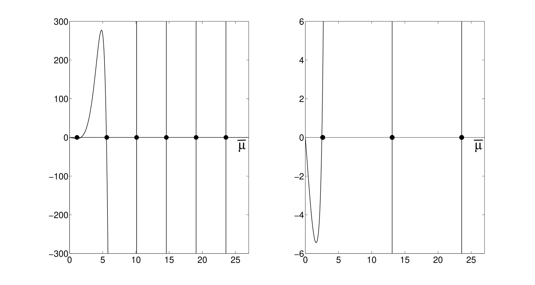
Figure 4: Plots of the function in the left member of (4.33) for two distinct values of ${x_{*}}$, namely ${x_{*}}=0.7$ (left panel) and ${x_{*}}=0.3$ (right panel). The solid dots mark the members of the sequence $\{(k+1/4)\pi\,{x_{*}}^{-1}\}_{k\geq 0}$. Note that the zeros of the plotted function approach this sequence rather quickly, with the quality of the approximation decreasing as ${x_{*}}\uparrow 1$. Indeed, in that regime, all exponentials appearing in (4.33) remain approximately equal for a large range of $\bar{\mu}-$values, and hence the first term becomes dominant only in the far range.

4.5 A second DCM pattern

So far, we have identified a DCM pattern corresponding to an $\Or(\varepsilon)$ biomass which is stabilized through a transcritical bifurcation at $\Lambda_{0}=0$ and destabilized through a secondary, Hopf bifurcation at an $\Or(1)$ value of $\Lambda_{0}$. Here, we show that, the system (4.4)–(4.6) admits a second, asymptotically larger, DCM-like steady state corresponding to an $\Or(\varepsilon^{1/2})$ biomass. We refrain from establishing the stability type, origins and eventual fate of that second steady state, reserving those problems to a later work.

We start by noting that the inclusion of the first higher order term in the formula for $a^{\prime}_{00k}$ reported in (4.1) yields

$$a^{\prime}_{00k}=-A^{\prime}_{k}(\Lambda_{0})\,A(\Lambda_{0})+\varepsilon^{1/2}\,\alpha\,\tilde{A}^{\prime}_{k}(\Lambda_{0}).$$

This formula is derived in Section 6.3, see (6.2) in particular. Here, the $\Lambda_{0}-$independent constants $\alpha$ and $\alpha^{\prime}$ were defined in (3.2) and (4.2), respectively, whereas the functions $a$ and $a^{\prime}$ are reported in (3.1) and (4.2). Also, $\tilde{A}^{\prime}_{k}(\Lambda_{0})=\tilde{\alpha}^{\prime}\,\tilde{a}^{\prime}(\Lambda_{0})\,\cos\left(\sqrt{N_{k}}\,{x_{*}}\right)$, with

$$\tilde{\alpha}^{\prime} = \frac{C_{1}\,C_{2}\,\sigma_{0}^{1/3}\,\sigma_{*}^{-1/2}}{\sqrt{2}\,f(0)},$$ (4.34)

$$\tilde{a}^{\prime}(\Lambda_{0}) = \frac{\sinh\left(\sqrt{\Lambda_{0}}\,(1-{x_{*}})\right)\,\int_{0}^{x_{*}}f(x)\,\cosh\left(\sqrt{\Lambda_{0}}\,x\right)\,dx}{\sqrt{\Lambda_{0}}\,\cosh\sqrt{\Lambda_{0}}}.$$ (4.35)

This formula for $\tilde{a}^{\prime}(\Lambda_{0})$ is also valid in a logarithmic regime for $\Lambda_{0}$, see (6.3) for details. Since the first term in the formula for $a^{\prime}_{00k}$ above decreases exponentially with $\Lambda_{0}$ (see (3.2)) whereas the second term decreases only algebraically, the two terms become asymptotically comparable for values of $\Lambda_{0}$ logarithmically large in $\varepsilon$, see Section 6 for details.

Replacing the formula for $a^{\prime}_{00k}$ in (4.1) by the formula above, substituting into (4.4)–(4.6), and working as in Section 4.2, we obtain the system

$$\begin{array}[]{rcl}\dot{\Omega}_{0}&=&\Lambda_{0}\Omega_{0}-A\,\Omega_{0}^{2}-B\,\Omega_{0}\sum_{m\geq 0}\Psi_{m}\ \ ,\\ \dot{\Psi}_{k}&=&-N_{k}\Psi_{k}+\left[(A^{\prime}_{k}\,A-\varepsilon^{1/2}\,\alpha\,\tilde{A}^{\prime}_{k})\,\Omega_{0}^{2}+A^{\prime}_{k}\,B\,\Omega_{0}\sum_{m\geq 0}\Psi_{m}\right].\end{array}$$ (4.36)

This is the analogue of (4.8) with the inclusion of higher order terms. The fixed points $(\Omega_{0}^{*},\Psi^{*})$ of this system are found, here again, by setting the left members to zero,

$$\begin{array}[]{rcll}\Lambda_{0}&=&A\,\Omega_{0}^{*}+B\sum_{m\geq 0}\Psi_{m}^{*}\ \ ,&{}\\ 0&=&-N_{k}\Psi_{k}^{*}+A^{\prime}_{k}\,\Lambda_{0}\,\Omega_{0}^{*}-\varepsilon^{1/2}\alpha\tilde{A}^{\prime}_{k}\,(\Omega_{0}^{*})^{2}.\end{array}$$ (4.37)

Solving the second equation for $\Psi_{k}^{*}$, we find an explicit expression for $\Psi_{k}^{*}$ in terms of $\Omega_{0}^{*}$,

$$\Psi_{k}^{*}=\frac{A^{\prime}_{k}}{N_{k}}\,\Lambda_{0}\,\Omega_{0}^{*}-\varepsilon^{1/2}\alpha\frac{\tilde{A}^{\prime}_{k}}{N_{k}}\,(\Omega_{0}^{*})^{2}.$$

Substituting this expression into the first equation in (4.37), we recover a singularly perturbed quadratic equation for $\Omega_{0}^{*}$,

$$\varepsilon^{1/2}\alpha B\left(\sum_{m\geq 0}\frac{\tilde{A}^{\prime}_{m}}{N_{m}}\right)(\Omega_{0}^{*})^{2}-\left(A+B\,\Lambda_{0}\,\sum_{m\geq 0}\frac{A^{\prime}_{m}}{N_{m}}\right)\,\Omega_{0}^{*}+\Lambda_{0}=0.$$ (4.38)

In Section 4.3.1, we obtained the formula

$$A+B\,\Lambda_{0}\,\sum_{m\geq 0}\frac{A^{\prime}_{m}}{N_{m}}=\alpha\,a(0),$$

while (4.16) yields

$$\sum_{m\geq 0}\frac{\tilde{A}^{\prime}_{m}}{N_{m}}=\tilde{\alpha}^{\prime}\,\tilde{a}^{\prime}(\Lambda_{0})\sum_{m\geq 0}\frac{\cos(\sqrt{N_{m}}\,{x_{*}})}{N_{m}}=\frac{a(0)}{2}\tilde{\alpha}^{\prime}\,\tilde{a}^{\prime}(\Lambda_{0}).$$

It follows that the quadratic equation yielding $\Omega_{0}^{*}$ can be recast as

$$\varepsilon^{1/2}\,\frac{\tilde{\alpha}^{\prime}\,B\,\tilde{a}^{\prime}(\Lambda_{0})}{2}\,(\Omega_{0}^{*})^{2}-\Omega_{0}^{*}+\frac{\Lambda_{0}}{\alpha\,a(0)}=0.$$

The two solutions of this equation are

$$\Omega_{0}^{*,\pm}=\varepsilon^{-1/2}\,\frac{1\pm\sqrt{1-2\varepsilon^{1/2}\,\tilde{\alpha}^{\prime}\,B\,\Lambda_{0}\,\tilde{a}^{\prime}(\Lambda_{0})/(\alpha\,a(0)})}{\tilde{\alpha}^{\prime}\,B\,\tilde{a}^{\prime}(\Lambda_{0})}=\Big{\{}\begin{array}[]{l}2\varepsilon^{-1/2}/(\tilde{\alpha}^{\prime}\,B\,\tilde{a}^{\prime}(\Lambda_{0})),\\ \Lambda_{0}/(\alpha\,a(0)),\end{array}$$

with the first one corresponding to the asymptotically larger DCM-pattern and the second one corresponding to the DCM-pattern identified trough our earlier work. We remark here that this first steady-state is, indeed, within the reach of our asymptotic methods, as $\Omega_{0}^{*}$ and $\Psi_{k}^{*}$ safely remain asymptotically smaller than the asymptotic bounds $\varepsilon^{-3/4}$ and $\varepsilon^{-1}$ for which our work in Section 2.3.1 remains valid. Note also that this steady state is a nonlinear function of $\Lambda_{0}$, with the distinguished limits

$$\lim_{\Lambda_{0}\to 0}\Omega_{0}^{*}(\Lambda_{0})=\frac{2\varepsilon^{-1/2}}{(1-{x_{*}})\,\tilde{\alpha}^{\prime}\,B\,\int_{0}^{x_{*}}f(x)\,dx}\quad\mbox{and}\quad\Omega_{0}^{*}(\Lambda_{0})=\frac{4\varepsilon^{-1/2}}{\ell\,\tilde{\alpha}^{\prime}\,B}\,\Lambda_{0},\ \mbox{as}\ \Lambda\to\infty.$$

In particular, this second pattern approaches a nonzero value as $\Lambda_{0}\downarrow 0$ and eventually grows linearly for $\Lambda_{0}\gg 1$.

5 An asymptotic formula for $b_{m00}$

In this section, we derive the asymptotic formula for $b_{m00}$ given in (4.1), where $m\in\mathbf{N}$ and

$$b_{m00}=(1-\nu)\int_{0}^{1}\,f(x)\,\zeta_{m}(x)\,\omega_{0}^{2}(x)\,dx.$$ (5.1)

As detailed earlier, the function $\omega_{0}$, appearing in (5.1), decays exponentially outside an $\Or(\varepsilon^{1/3})-$neighborhood of the origin (cf. (A.1)), whereas the period of the sinusoidal term $\zeta_{m}$ is equal to $2\pi/\sqrt{N_{m}}=4/(2m+1)$. Below, we analyze the three different regimes—in which the integrand is predominantly localized, concurrently localized and oscillatory, and predominantly oscillatory—and we derive the leading order, uniform asymptotic expansion

$$b_{m00}=\left\{\begin{array}[]{l}\displaystyle b,\quad\mbox{for}\ m\ll\varepsilon^{-1/3},\vspace*{0.2cm}\\ \displaystyle b\,C_{1}^{2}\int_{0}^{\infty}\cos\left(\frac{\varepsilon^{1/3}\,\sqrt{N_{m}}\,\tau}{\sigma_{0}^{1/3}}\right){\rm Ai}^{2}\left(\tau+A_{1}\right)\,d\tau,\quad\mbox{for}\ m=\Or(\varepsilon^{-1/3}),\vspace*{0.2cm}\\ \displaystyle-b\,\frac{6\,C_{3}\,C_{1}^{2}\,\sigma_{0}^{2}}{\varepsilon\,N_{m}^{2}\,f(0)},\quad\mbox{for}\ m\gg\varepsilon^{-1/3}.\end{array}\right.$$ (5.2)

Here, $b=\sqrt{2}\,(1-\nu)\,f(0)$, cf. Section 4.1.

5.1 The case $m\ll\varepsilon^{-1/3}$

Here, $2\pi/\sqrt{N_{m}}\gg\varepsilon^{1/3}$ and hence the integrand is predominantly localized around $x=0$. Thus, $\zeta_{m}$ may be approximated to leading order by $\zeta_{m}(0)=\sqrt{2}$ in that neighborhood. Since $\|\omega_{0}\|_{2}=1$ (cf. our discussion in Sections 2.1–2.2), we obtain the desired formula

$$b_{m00}\sim b.$$ (5.3)

5.2 The case $m=\Or(\varepsilon^{-1/3})$

Here, $2\pi/\sqrt{N_{m}}=\Or(\varepsilon^{1/3})$, and hence the neighborhood of the origin outside which $\omega_{0}$ decays exponentially and the period of the sinusoidal term are of the same asymptotic magnitude. Defining the new variable $\tau=\tau_{1}\,x$ in (5.1), with $\tau_{1}=\left|A_{1}\right|/x_{0}$ (2.17), we obtain

$$b_{m00}=\frac{\sqrt{2}\,(1-\nu)}{\tau_{1}}\int_{0}^{\tau_{1}}f\left(\frac{\tau}{\tau_{1}}\right)\,\cos\left(\sqrt{N_{m}}\,\frac{\tau}{\tau_{1}}\right)\,\omega_{0}^{2}\left(\frac{\tau}{\tau_{1}}\right)\,d\tau.$$ (5.4)

Now, (A.1) yields, to leading order and for any $\tau_{0}\ll\varepsilon^{-1/3}$,

$$\omega_{0}\left(\frac{\tau}{\tau_{1}}\right)=\left\{\begin{array}[]{l}\varepsilon^{-1/6}\,C_{1}\,\sigma_{0}^{1/6}{\rm Ai}\left(\tau+A_{1}\right),\hskip 120.92421pt\quad\mbox{for}\ \tau\in[0,-A_{1}),\\ \frac{\varepsilon^{-1/12}\,C_{1}\,C_{2}\,\sigma_{0}^{1/3}}{2\sqrt{\pi}\,F^{1/4}(\tau/\tau_{1})}\,\exp\left(-\frac{1}{\sqrt{\varepsilon}\tau_{1}}\int_{0}^{\tau+A_{1}}\sqrt{F(\frac{t}{\tau_{1}}+x_{0})-F(x_{0})}\,dt\right),\\ \hskip 256.0748pt\mbox{for}\ \tau\in(-A_{1},\tau_{0}],\end{array}\right.$$

where we have also changed the integration variable by means of $s=t/\tau_{1}+x_{0}$. These two formulas agree—as, indeed, they should by construction—in the regime $1\ll\tau_{0}\ll\varepsilon^{-1/3}$. Indeed, recalling the asymptotic expansion of ${\rm Ai}$ in a neighborhood of infinity [2], we find that the first branch of the formula above yields

$$\varepsilon^{-1/6}\,\frac{C_{1}\,\sigma_{0}^{1/6}}{2\,\sqrt{\pi}\,\tau^{1/4}}\,\exp\left(-\frac{2}{3}(\tau+A_{1})^{3/2}\right).$$

Similarly, the formula in the case $\tau\in(\left|A_{1}\right|,\tau_{0}]$ becomes, upon Taylor-expanding $F$,

$$\varepsilon^{-1/12}\,\frac{C_{1}\,C_{2}\,\sigma_{0}^{1/12}\,\tau_{1}^{1/4}}{2\sqrt{\pi}\,\tau^{1/4}}\,\exp\left(-\frac{2}{3}\sqrt{\frac{\sigma_{0}}{\varepsilon}}\left(\frac{\tau+A_{1}}{\tau_{1}}\right)^{3/2}\right).$$

That the two formulas agree now follows from the definition $\tau_{1}=\left|A_{1}\right|/x_{0}$ and the formulas (2.17) and (3.3) for $x_{0}$ and $C_{2}$. Hence, we may write

$$\omega_{0}\left(\frac{\tau}{\tau_{1}}\right)\sim\varepsilon^{-1/6}\,C_{1}\,\sigma_{0}^{1/6}{\rm Ai}\left(\tau+A_{1}\right),\quad\mbox{for}\quad\tau\ll\varepsilon^{-1/3}.$$

Since the contribution to the integral in (5.4) of greater values of $\tau$ may be estimated to be exponentially small, we can write

$$b_{m00} = \varepsilon^{-1/3}\,\frac{\sqrt{2}\,(1-\nu)\,C_{1}^{2}\,\sigma_{0}^{1/3}}{\tau_{1}}\int_{0}^{\infty}\,f\left(\frac{\tau}{\tau_{1}}\right)\,\cos\left(\sqrt{N_{m}}\,\frac{\tau}{\tau_{1}}\right)\,{\rm Ai}^{2}\left(\tau+A_{1}\right)\,d\tau$$ (5.5)

$$= b\,C_{1}^{2}\int_{0}^{\infty}\,\cos\left(\frac{\varepsilon^{1/3}\,\sqrt{N_{m}}\,\tau}{\sigma_{0}^{1/3}}\right)\,{\rm Ai}^{2}\left(\tau+A_{1}\right)\,d\tau,$$

to leading order, as desired. Note that this formula reduces to (5.3), for $m\ll\varepsilon^{-1/3}$.

5.3 The case $m\gg\varepsilon^{-1/3}$

Here, $2\pi/\sqrt{N_{m}}\ll\varepsilon^{1/3}$. Similarly to our work in the previous section, we define the new variable $\tau=\varepsilon^{-1/3}x$. We find, then,

$$b_{m00}=\sqrt{2}\,\varepsilon^{1/3}\,(1-\nu)\int_{0}^{\varepsilon^{-1/3}}\,g(\tau)\,\cos\left(\varepsilon^{1/3}\,\sqrt{N_{m}}\,\tau\right)\,d\tau,$$

where $g(\tau)=f\left(\varepsilon^{1/3}\tau\right)\,\omega_{0}^{2}\left(\varepsilon^{1/3}\tau\right)$. Using Theorem D.4 (with $\lambda=\varepsilon^{1/3}\,\sqrt{N_{m}}$, $\Phi(t)=t=\tau$, and $h(\tau)=g(\tau)$) and the fact that the right-boundary term is exponentially smaller than the left one, as $\omega_{0}(1)$ is exponentially smaller than $\omega_{0}(0)$ (cf. A), we obtain

$$b_{m00} = \sqrt{2}\,\varepsilon^{1/3}\,(1-\nu)\,{\rm Re}\left(\sum_{k=0}^{\infty}g^{(k)}(0)\left(\frac{{\rm i}}{\varepsilon^{1/3}\,\sqrt{N_{m}}}\right)^{k+1}\right)$$ (5.6)

$$= \sqrt{2}\,\frac{1-\nu}{\varepsilon^{1/3}\,N_{m}}\,\sum_{k=0}^{\infty}(-1)^{k+1}g^{(2k+1)}(0)\left(\frac{1}{\varepsilon^{1/3}\,\sqrt{N_{m}}}\right)^{2k}.$$

Recalling the definition of $g$, and employing (A.1) and that ${\rm Ai}(A_{1})={\rm Ai}^{\prime\prime}(A_{1})=0$, we calculate

$$g^{\prime}(0)=0\quad\mbox{and}\quad g^{\prime\prime\prime}(0)=-6\,[{\rm Ai}^{\prime}(A_{1})]^{2}\,C_{1}^{2}\,\sigma_{0}^{2}.$$

The desired result now follows, while (5.6) also reduces to (5.5) for $m=\Or(\varepsilon^{-1/3})$.

6 An asymptotic formula for $a^{\prime}_{00k}$

In this section, we derive the asymptotic formula for $a^{\prime}_{00k}$ for $\Or(1)$ values of $\Lambda_{0}$ collected in (4.1),

$$a^{\prime}_{00k}=-A^{\prime}_{k}(\Lambda_{0})\,A(\Lambda_{0}),\quad\mbox{for}\ 0\neq k\ll\varepsilon^{-1/3}.$$ (6.1)

Further, we extend this result to

$$a^{\prime}_{00k}=-\left(A^{\prime}_{k}(\Lambda_{0})\,A(\Lambda_{0})-\varepsilon^{1/2}\,\alpha\,\tilde{A}^{\prime}_{k}(\Lambda_{0})\right),\quad\mbox{for}\ 0\neq k\ll\varepsilon^{-1/3},$$ (6.2)

which remains valid at least in the regime

$$\Lambda_{0}=\frac{1}{4{x_{*}}^{2}}\log^{2}\varepsilon+\frac{1}{{x_{*}}^{2}}\log\varepsilon\log(-\log\varepsilon)+\frac{1}{{x_{*}}^{2}}\log^{2}\log\varepsilon+\mu\log\varepsilon,$$ (6.3)

for all $\mu\in(-\infty,\mu_{0}]$ and $\mu_{0}>0$ any $\Or(1)$ value. Here, $A(\Lambda_{0})=\alpha\,a(\Lambda_{0})$, $A^{\prime}_{k}(\Lambda_{0})=\alpha^{\prime}\,a^{\prime}_{k}(\Lambda_{0})$, and $\tilde{A}^{\prime}_{k}(\Lambda_{0})=\tilde{\alpha}^{\prime}\,\tilde{a}^{\prime}(\Lambda_{0})$. The $\Lambda_{0}-$independent constants $\alpha$, $\alpha^{\prime}$, and $\tilde{\alpha}^{\prime}$ were defined in (3.2), (4.2), and (4.34), respectively, whereas the functions $a$, $a^{\prime}$, and $\tilde{a}^{\prime}$ are reported in (3.1), (4.2), and (4.35). We remark, here, that these results are only valid for those values of $k$ for which $\zeta_{k}({x_{*}})\neq 0$. For the remaining values of $k$, Theorem D.1 yields (algebraically) higher order results. Also, we note that asymptotic formulas for higher values of $k$ can be derived as in the previous section, albeit at considerable extra computational cost.

We first write out explicitly the expression for $a^{\prime}_{00k}$ yielded by (2.21),

$$a^{\prime}_{00k}=\varepsilon^{-1/3}\delta\int_{0}^{1}a_{0}(x)\,\omega_{0}(x)\,\psi_{k}(x)\,dx+\varepsilon^{2/3}\delta\ell^{-1}\int_{0}^{1}a_{0}(x)\,\omega^{+}_{0}(x)\,\zeta_{k}(x)\,dx.$$

Recalling the definition of $a_{0}$ from (2.22) and working as in Section 3, we obtain further

$$a^{\prime}_{00k}= \varepsilon^{-1/3}\delta^{2}\int_{0}^{1}\int_{0}^{x}h_{1}(x,y)\,\omega^{+}_{0}(y)\,\omega_{0}(x)\,\psi_{k}(x)\,dydx$$

$$+\varepsilon^{-1/3}\delta^{2}\int_{0}^{1}\int_{0}^{1}h_{2}(x,y)\,\omega^{+}_{0}(y)\,\omega_{0}(x)\,\psi_{k}(x)\,dydx$$

$$+\varepsilon^{2/3}\delta^{2}\ell^{-1}\int_{0}^{1}\int_{0}^{x}h_{1}(x,y)\,\zeta_{k}(x)\,\omega^{+}_{0}(y)\,\omega^{+}_{0}(x)\,dydx$$

$$+\varepsilon^{2/3}\delta^{2}\ell^{-1}\int_{0}^{1}\int_{0}^{1}h_{2}(x,y)\,\zeta_{k}(x)\,\omega^{+}_{0}(y)\,\omega^{+}_{0}(x)\,dydx.$$

Substituting, finally, from (C.25), we obtain an integral formula for $a^{\prime}_{00k}$ which is amenable to the sort of asymptotic analysis employed in Sections 3 and 5,

$$a^{\prime}_{00k}= \frac{\varepsilon^{-1/3}\delta^{2}}{\ell}\left[(W_{\psi})^{-1}\int_{0}^{1}\int_{0}^{x}\int_{0}^{x}h_{1,k}(x,y,z)\,\omega_{0}(x)\,\psi_{k,-}(x)\,\omega^{+}_{0}(y)\,\psi^{+}_{k,+}(z)\,dzdydx\right.$$ (6.4)

$$+(W_{\psi})^{-1}\int_{0}^{1}\int_{0}^{1}\int_{0}^{x}h_{2,k}(x,y,z)\,\omega_{0}(x)\,\psi_{k,-}(x)\,\omega^{+}_{0}(y)\,\psi^{+}_{k,+}(z)\,dzdydx$$

$$-(W_{\psi})^{-1}D_{k}(0)\int_{0}^{1}\int_{0}^{x}\int_{0}^{1}h_{1,k}(x,y,z)\,\omega_{0}(x)\,\psi_{k,-}(x)\,\omega^{+}_{0}(y)\,\psi^{+}_{k,-}(z)\,dzdydx$$

$$-(W_{\psi})^{-1}D_{k}(0)\int_{0}^{1}\int_{0}^{1}\int_{0}^{1}h_{2,k}(x,y,z)\,\omega_{0}(x)\,\psi_{k,-}(x)\,\omega^{+}_{0}(y)\,\psi^{+}_{k,-}(z)\,dzdydx$$

$$+(W_{\psi})^{-1}\int_{0}^{1}\int_{0}^{x}\int_{x}^{1}h_{1,k}(x,y,z)\,\omega_{0}(x)\,\psi_{k,+}(x)\,\omega^{+}_{0}(y)\,\psi^{+}_{k,-}(z)\,dzdydx$$

$$+(W_{\psi})^{-1}\int_{0}^{1}\int_{0}^{1}\int_{x}^{1}h_{2,k}(x,y,z)\,\omega_{0}(x)\,\psi_{k,+}(x)\,\omega^{+}_{0}(y)\,\psi^{+}_{k,-}(z)\,dzdydx$$

$$+\varepsilon\int_{0}^{1}\int_{0}^{x}h_{1}(x,y)\,\zeta_{k}(x)\,\omega^{+}_{0}(x)\,\omega^{+}_{0}(y)\,dydx$$

$$\left.+\varepsilon\int_{0}^{1}\int_{0}^{1}h_{2}(x,y)\,\zeta_{k}(x)\,\omega^{+}_{0}(x)\,\omega^{+}_{0}(y)\,dydx\right].$$

Here, $h_{i,k}(x,y,z)=h_{i}(x,y)\,f(z)\,\zeta_{k}(z)$, for $i=1,2$, and the constants $D_{k}(0)$ are reported in (C.23)–(C.24). Let $\mathcal{I}_{1},\ldots,\mathcal{I}_{8}$ denote the integrals in the right member of (6.4) in the order that they appear (the three-dimensional domains of integration for $\mathcal{I}_{1},\ldots,\mathcal{I}_{6}$ are sketched in Figure 5). In what follows, we omit the term $\theta\,\omega^{2}_{0,-}(1;x_{0})\,\omega_{0,+}(x;x_{0})$ in the expression (A.1) for $\omega_{0}$, as one can show that its contribution is exponentially small compared to the leading order terms (see also Sections 3 and 5).

Figure 5: The domains of integration for the integrals $\mathcal{I}_{1},\ldots,\mathcal{I}_{6}$ in (6.4).

6.1 A rewrite of (6.4)

In this section, we group together integrals appearing in the right member of (6.4) in order to achieve a first reduction in the numbers of terms of that member. We start with rewriting the term $-(W_{\psi})^{-1}\,D_{k}(0)\,\mathcal{I}_{4}+(W_{\psi})^{-1}\,\mathcal{I}_{6}+\varepsilon\,\mathcal{I}_{8}$. First,

$$\mathcal{I}_{4}=\int\int_{\pi_{x}D_{4}}\left(\int_{0}^{1}h_{2,k}(x,y,z)\,\omega_{0}(x)\,\psi_{k,-}(x)\,dx\right)\omega^{+}_{0}(y)\,\psi^{+}_{k,-}(z)\,dA_{yz},$$

where $\pi_{x}$ is the orthogonal projection on the $yz-$plane—and hence $\pi_{x}D_{4}=[0,1]^{2}$—and $dA_{yz}$ is the area element on that plane. Since $\psi_{k,-}=\varepsilon^{1/3}C_{1}^{-1}\sigma_{0}^{-1/3}\omega_{0}$ in a neighborhood of the origin (cf. (A.1) and (C.14)), $\omega_{0}$ is exponentially small outside this neighborhood, and $\|\omega_{0}\|_{2}=1$, we write

$$\mathcal{I}_{4} = \varepsilon^{1/3}\,C_{1}^{-1}\,\sigma_{0}^{-1/3}\,\int\int_{\pi_{x}D_{4}}h_{2,k}(0,y,z)\,\omega^{+}_{0}(y)\,\psi^{+}_{k,-}(z)\,dA_{yz}.$$

Recalling that $\psi^{+}_{k,-}=E\,\psi_{k,-}$, according to our convention in Section 2, and substituting into the formula above from (A.2) and (C.14), we obtain

$$\mathcal{I}_{4} = \varepsilon^{1/2}\,\frac{C_{2}^{2}}{4\pi}\,\int\int_{\pi_{x}D_{4}}\frac{h_{2,k}(0,y,z)}{F^{1/4}(y)\,F^{1/4}(z)}\,\exp\left(\frac{J_{-}(y)+J_{-}(z)}{\sqrt{\varepsilon}}\right)\,dA_{yz},$$

whence, employing also (C.23), we find

$$(W_{\psi})^{-1}\,D_{k}(0)\,\mathcal{I}_{4}=\varepsilon^{-1/6}\,\int\int_{\pi_{x}D_{4}}\Xi_{4}(y,z)\,\exp\left(\frac{\Pi_{4}(y,z)}{\sqrt{\varepsilon}}\right)\,dA_{yz}.$$ (6.5)

Here,

$$\Xi_{4}(y,z)=\frac{C_{2}^{2}\,d_{k}}{4\pi\,W_{\psi}}\,\frac{h_{2}(0,y)\,f(z)\,\zeta_{k}(z)}{F^{1/4}(y)\,F^{1/4}(z)}\quad\mbox{and}\quad\Pi_{4}(y,z)=J_{-}(y)+J_{-}(z).$$ (6.6)

Next, we rewrite $\mathcal{I}_{6}$,

$$(W_{\psi})^{-1}\,\mathcal{I}_{6}=(W_{\psi})^{-1}\,\int\int_{\pi_{x}D_{6}}\left(\int_{0}^{z}h_{2,k}(x,y,z)\,\omega_{0}(x)\,\psi_{k,+}(x)\,dx\right)\,\omega^{+}_{0}(y)\,\psi^{+}_{k,-}(z)\,dA_{yz}.$$

Employing (A.1) and (C.17), now, we obtain

$$(W_{\psi})^{-1}\,\mathcal{I}_{6}=\varepsilon^{1/6}\,\frac{C_{1}\,\sigma_{0}^{1/3}}{2\pi\,W_{\psi}}\,\int\int_{\pi_{x}D_{6}}\left(\int_{0}^{z}\frac{h_{2,k}(x,y,z)}{\sqrt{F(x)}}dx\right)\omega^{+}_{0}(y)\,\psi^{+}_{k,-}(z)\,dA_{yz}.$$

Further using (A.2) and, once again, (C.17), we find

$$(W_{\psi})^{-1}\,\mathcal{I}_{6}=\varepsilon^{1/3}\,\int\int_{\pi_{x}D_{6}}\Xi_{6}(y,z)\,\exp\left(\frac{\Pi_{6}(y,z)}{\sqrt{\varepsilon}}\right)dA_{yz}.$$ (6.7)

Here, ${\pi_{x}D_{6}}={\pi_{x}D_{4}}$, $\Pi_{6}(y,z)=\Pi_{4}(y,z)$, and

$$\Xi_{6}(y,z)=\frac{C_{1}^{2}\,C_{2}^{2}\,\sigma_{0}^{2/3}}{8\pi^{2}\,W_{\psi}}\,\frac{f(z)\,\zeta_{k}(z)}{F^{1/4}(y)\,F^{1/4}(z)}\,\int_{0}^{z}\frac{h_{2}(x,y)}{\sqrt{F(x)}}\,dx.$$ (6.8)

Similarly, renaming $(x,y)$ as $(y,z)$ in $\mathcal{I}_{8}$, we derive the formula

$$\varepsilon\,\mathcal{I}_{8}=\varepsilon^{5/6}\,\int\int_{D_{8}}\Xi_{8}(y,z)\,\exp\left(\frac{\Pi_{8}(y,z)}{\sqrt{\varepsilon}}\right)\,dA_{yz},$$ (6.9)

where $D_{8}=\pi_{x}D_{6}=\pi_{x}D_{4}$, $\Pi_{8}(y,z)=\Pi_{6}(y,z)=\Pi_{4}(y,z)$, and

$$\Xi_{8}(y,z)=\frac{C_{1}^{2}\,C_{2}^{2}\,\sigma_{0}^{2/3}}{4\pi}\,\frac{h_{2}(y,z)\,\zeta_{k}(y)}{F^{1/4}(y)\,F^{1/4}(z)}.$$ (6.10)

Combining (6.5)–(6.10), we obtain

$$-(W_{\psi})^{-1}\,D_{k}(0)\,\mathcal{I}_{4}+(W_{\psi})^{-1}\,\mathcal{I}_{6}+\mathcal{I}_{8}$$

$$=-\varepsilon^{-1/6}\,\int\int_{\pi_{x}D_{4}}\tilde{\Xi}_{4}(y,z)\,\exp\left(\frac{\Pi_{4}(y,z)}{\sqrt{\varepsilon}}\right)\,dA_{yz},$$ (6.11)

where, to leading order, uniformly over ${\pi_{x}D_{4}}$, and for all $\Or(1)$ values of $\Lambda_{0}$,

$$\tilde{\Xi}_{4}(y,z)=\Xi_{4}(y,z)=\frac{C_{2}^{2}\,d_{k}}{4\pi\,W_{\psi}}\frac{h_{2}(0,y)\,f(z)\,\zeta_{k}(z)}{F^{1/4}(y)\,F^{1/4}(z)}.$$ (6.12)

Next, we rewrite the term $(W_{\psi})^{-1}\mathcal{I}_{5}+\varepsilon\,\mathcal{I}_{7}$. We write first

$$\mathcal{I}_{5} = \int\int_{\pi_{x}D_{5}}\left(\int_{y}^{z}h_{1,k}(x,y,z)\,\omega_{0}(x)\,\psi_{k,+}(x)\,dx\right)\,\omega^{+}_{0}(y)\,\psi^{+}_{k,-}(z)\,dA_{yz},$$

where $\pi_{x}D_{5}=\{(y,z)|0\leq y\leq z,\,0\leq z\leq 1\}$. Now, (A.1)–(A.2) and (C.14) yield further

$$(W_{\psi})^{-1}\,\mathcal{I}_{5} = \varepsilon^{1/6}\,\frac{C_{1}\,C_{2}\,\sigma_{0}^{1/3}}{2\pi\,W_{\psi}}\,\int\int_{\pi_{x}D_{5}}\left(\int_{y}^{z}\frac{h_{1,k}(x,y,z)}{\sqrt{F(x)}}\,dx\right)\omega^{+}_{0}(y)\,\psi^{+}_{k,-}(z)\,dA_{yz}$$ (6.13)

$$= \varepsilon^{1/3}\,\int\int_{\pi_{x}D_{5}}\Xi_{5}(y,z)\,\exp\left(\frac{\Pi_{5}(y,z)}{\sqrt{\varepsilon}}\right)dA_{yz},$$

where we have defined the functions

$$\Xi_{5}(y,z)=\frac{C_{1}^{2}\,C_{2}^{3}\,\sigma_{0}^{2/3}}{8\pi^{2}\,W_{\psi}}\,\frac{f(z)\,\zeta_{k}(z)}{F^{1/4}(y)\,F^{1/4}(z)}\,\int_{y}^{z}\frac{h_{1}(x,y)}{\sqrt{F(x)}}\,dx$$ (6.14)

and $\Pi_{5}(y,z)=\Pi_{4}(y,z)$. Next, renaming $x$ into $z$ in $\mathcal{I}_{7}$, we find

$$\varepsilon\,\mathcal{I}_{7}=\varepsilon^{5/6}\,\int\int_{D_{7}}\Xi_{7}(y,z)\,\exp\left(\frac{\Pi_{7}(y,z)}{\sqrt{\varepsilon}}\right)\,dA_{yz},$$ (6.15)

where

$$D_{7}=\pi_{x}D_{5},\quad\Xi_{7}(y,z)=\frac{C_{1}^{2}\,C_{2}^{2}\,\sigma_{0}^{2/3}}{4\pi}\,\frac{h_{1}(z,y)\,\zeta_{k}(z)}{F^{1/4}(y)\,F^{1/4}(z)},\quad\mbox{and}\quad\Pi_{7}(y,z)=\Pi_{4}(y,z).$$ (6.16)

Combining (6.13)–(6.16), we find, to leading order and uniformly over $D_{8}$,

$$(W_{\psi})^{-1}\,\mathcal{I}_{5}+\varepsilon\,\mathcal{I}_{7}=\varepsilon^{1/3}\,\int\int_{D_{7}}\tilde{\Xi}_{5}(y,z)\,\exp\left(\frac{\Pi_{4}(y,z)}{\sqrt{\varepsilon}}\right)\,dA_{yz},$$ (6.17)

where $\tilde{\Xi}_{5}(y,z)=\Xi_{5}(y,z)+\varepsilon^{1/2}\,\Xi_{7}(y,z)$.

We now rewrite $(W_{\psi})^{-1}\mathcal{I}_{2}$. First,

$$\mathcal{I}_{2}=\int\int_{\pi_{y}D_{2}}\tilde{H}_{2}(x)\,f(z)\,\zeta_{k}(z)\,\omega_{0}(x)\,\psi_{k,-}(x)\,\psi^{+}_{k,+}(z)\,dA_{xz},$$

where $\tilde{H}_{2}(x)=\int_{0}^{1}h_{2}(x,y)\,\omega^{+}_{0}(y)\,dy$. Substituting for $\omega^{+}_{0}(y)$ from (A.2), we find further

$$\mathcal{I}_{2}=\varepsilon^{-1/12}\,\frac{C_{1}C_{2}\sigma_{0}^{1/3}}{2\sqrt{\pi}}\,\int\int_{\pi_{y}D_{2}}H_{2}(x)\,\omega_{0}(x)\,\psi_{k,-}(x)\,f(z)\,\zeta_{k}(z)\,\psi^{+}_{k,+}(z)\,dA_{xz},$$

where $H_{2}(x)=\int_{0}^{1}h_{2}(x,y)\,F^{-1/4}(y)\,\exp(J_{-}(y)/\sqrt{\varepsilon})\,dy$. Using Theorem D.1, now, we obtain

$$(W_{\psi})^{-1}\,\mathcal{I}_{2} =\varepsilon^{1/6}\delta^{-1}\,C^{\prime\prime}_{2}\int\int_{\pi_{y}D_{2}}h_{2}(x,{x_{*}})\,\omega_{0}(x)\,\psi_{k,-}(x)\,f(z)\,\zeta_{k}(z)\,\psi^{+}_{k,+}(z)\,dA_{xz}$$ (6.18)

$$=\varepsilon^{7/12}\,\int\int_{\pi_{y}D_{2}}\Xi_{2}(x,z)\,\exp\left(\frac{\Pi_{2}(x,z)}{\sqrt{\varepsilon}}\right)\,dA_{xz},$$

where $C^{\prime\prime}_{2}$ is an $\Or(1)$ constant, $\pi_{y}D_{2}=\{(x,z)|0\leq z\leq x,\,0\leq x\leq 1\}$, $\Pi_{2}(x,z)=J_{-}({x_{*}})+J_{+}(z)-2I(x)$,

$$\Xi_{2}(x,z)=C^{\prime}_{2}\,\frac{h_{2}(x,{x_{*}})\,f(z)\,\zeta_{k}(z)}{\sqrt{F(x)}\,F^{1/4}(z)},\quad\mbox{with $C^{\prime}_{2}$ an $\Or(1)$ constant.}\$$ (6.19)

Finally, we rewrite $(W_{\psi})^{-1}D_{k}(0)\,\mathcal{I}_{3}$. First,

$$\mathcal{I}_{3} = \left(\int_{0}^{1}f(z)\,\zeta_{k}(z)\,\psi^{+}_{k,-}(z)\,dz\right)\int\int_{\pi_{z}D_{3}}h_{1}(x,y)\,\omega_{0}(x)\,\psi_{k,-}(x)\,\omega^{+}_{0}(y)\,dA_{xy}.$$

Substituting from (A.1)–(A.2) and (C.14) into this formula and interchanging the roles of $y$ and $z$ in the single and double integrals, we find

$$(W_{\psi})^{-1}\,D_{k}(0)\,\mathcal{I}_{3}=\varepsilon^{-1/3}\,\tilde{I}_{3}\,\int\int_{\pi_{y}D_{2}}\tilde{\Xi}_{3}(x,z)\,\exp\left(\frac{\tilde{\Pi}_{3}(x,z)}{\sqrt{\varepsilon}}\right)\,dA_{xz},$$ (6.20)

where $\tilde{I}_{3}=\int_{0}^{1}F^{-1/4}(y)\,f(y)\,\zeta_{k}(y)\,\exp\left(J_{-}(y)/\sqrt{\varepsilon}\right)\,dy$ and

$$\tilde{\Xi}_{3}(x,z)=\tilde{C}_{3}\,\frac{h_{1}(x,z)}{\sqrt{F(x)}\,F^{1/4}(z)}\quad\mbox{and}\quad\tilde{\Pi}_{3}(x,z)=J_{-}(z)-2I(x),$$ (6.21)

for some $\Or(1)$ constant $\tilde{C}_{3}$.

6.2 An asymptotic estimate for $a^{\prime}_{00k}$ in the regime $\Lambda_{0}=\Or(1)$

In this section, we estimate the various terms derived above, starting from $-(W_{\psi})^{-1}\,D_{k}(0)\,\mathcal{I}_{4}+(W_{\psi})^{-1}\,\mathcal{I}_{6}+\varepsilon\,\mathcal{I}_{8}$ (cf. (6.11)–(6.12)). The exponent $\Pi_{4}$ becomes maximum at the interior critical point $({x_{*}},{x_{*}})$, and thus Theorem D.1 yields

$$-(W_{\psi})^{-1}\,D_{k}(0)\,\mathcal{I}_{4}+(W_{\psi})^{-1}\,\mathcal{I}_{6}+\mathcal{I}_{8} =-\varepsilon^{1/2}\frac{2\pi}{\left|J^{\prime\prime}_{-}({x_{*}})\right|}\,\left(\varepsilon^{-1/6}\,\tilde{\Xi}_{4}({x_{*}},{x_{*}})\,\exp\left(\frac{\Pi_{4}({x_{*}},{x_{*}})}{\sqrt{\varepsilon}}\right)\right)$$

$$=-\varepsilon^{1/3}\,\delta^{-2}\,\tilde{C}_{4},$$

where

$$\tilde{C}_{4} = C_{2}^{2}\,(\sigma_{*}W_{\psi})^{-1}\,d_{k}\,\zeta_{k}({x_{*}})\,f({x_{*}})\,\,h_{2}(0,{x_{*}}).$$

Next, we estimate $(W_{\psi})^{-1}\,\mathcal{I}_{5}+\varepsilon\,\mathcal{I}_{7}$, cf. (6.17). The sole (quadratic) maximum of $\Pi_{4}$ in $D_{7}$ lies at the critical point $({x_{*}},{x_{*}})\in\partial D_{7}$, where $\tilde{\Xi}_{5}({x_{*}},{x_{*}})=0$ and $\tilde{\Xi}_{7}({x_{*}},{x_{*}})\neq 0$. Recalling the definition of $\tilde{\Xi}_{5}$ and employing Theorem D.1, then, we obtain

$$(W_{\psi})^{-1}\,\mathcal{I}_{5}+\mathcal{I}_{7}=\varepsilon\left(\varepsilon^{1/3}\,C_{0}\,\exp\left(\frac{\Pi_{4}({x_{*}},{x_{*}})}{\sqrt{\varepsilon}}\right)\right)=\varepsilon^{4/3}\delta^{-2}\,\tilde{C}_{7},$$

for some $\Or(1)$ constants $C_{0}$ and $\tilde{C}_{7}$.

We now estimate the remaining three integrals starting with $(W_{\psi})^{-1}\,\mathcal{I}_{2}$, cf. (6.18)–(6.19). The exponent $\Pi_{2}$ has a sole maximum at the point $({x_{*}},{x_{*}})\in\partial(\pi_{y}D_{2})$ which is not a critical point (compare to the maximization of $\Pi_{4}$ in Section 3). Hence, Theorem D.1 yields

$$(W_{\psi})^{-1}\,\mathcal{I}_{2}=\varepsilon^{3/4}\,C^{\prime\prime\prime}_{2}\left(\varepsilon^{7/12}\,\Xi_{2}({x_{*}},{x_{*}})\,\exp\left(\frac{\Pi_{2}({x_{*}},{x_{*}})}{\sqrt{\varepsilon}}\right)\right)=\varepsilon^{4/3}\,\delta^{-2}\,C_{2},$$

for some $\Or(1)$ constants $C^{\prime\prime\prime}_{2}$ and $C_{2}$. Next, since $D_{1}\subset D_{2}$ and the integrands of $\mathcal{I}_{1}$ and $\mathcal{I}_{2}$ differ only by an $\Or(1)$ multiple, the above analysis also yields that $(W_{\psi})^{-1}\mathcal{I}_{1}$ is at most of the same order as $(W_{\psi})^{-1}\mathcal{I}_{2}$. Finally, we estimate $(W_{\psi})^{-1}\,D_{k}(0)\,\mathcal{I}_{3}$, cf. (6.20)–(6.21). First, we estimate

$$\tilde{I}_{3}=\int_{0}^{1}\frac{f(y)\,\zeta_{k}(y)}{F^{1/4}(y)}\,\exp\left(\frac{J_{-}(y)}{\sqrt{\varepsilon}}\right)\,dy=\varepsilon^{1/4}\,\delta^{-1}\,C^{\prime\prime}_{3},$$

for some $\Or(1)$ constant $C^{\prime\prime}_{3}$. Substituting into (6.20), then, we obtain

$$(W_{\psi})^{-1}\,D_{k}(0)\,\mathcal{I}_{3} = \varepsilon^{-1/12}\,\int\int_{\pi_{y}D_{2}}\Xi_{3}(x,z)\,\exp\left(\frac{\Pi_{3}(x,z)}{\sqrt{\varepsilon}}\right)\,dA_{xz},$$

where

$$\Xi_{3}(x,z)=\tilde{C}^{\prime}_{3}\,\frac{h_{1}(x,z)}{\sqrt{F(x)}\,F^{1/4}(z)}\quad\mbox{and}\quad\Pi_{3}(x,z)=J_{-}({x_{*}})+J_{-}(z)-2I(x),$$

for some $\Or(1)$ constant $\tilde{C}^{\prime}_{3}$. The exponent $\Pi_{3}$ has a sole maximum at the point $({x^{**}},{x^{**}})\in\partial(\pi_{y}D_{2})$ which is also not a critical point (compare to the maximization of $\Pi_{1}$ in Section 3). Hence, Theorem D.1 yields

$$(W_{\psi})^{-1}\,D_{k}(0)\,\mathcal{I}_{3} = \varepsilon^{3/4}C^{\prime}_{3}\left(\varepsilon^{-1/12}\Xi_{3}({x_{*}},{x_{*}})\exp\left(\frac{\Pi_{3}({x_{*}},{x_{*}})}{\sqrt{\varepsilon}}\right)\right)$$

$$= \varepsilon^{2/3}C_{3}\exp\left(\frac{\Pi_{3}({x^{**}},{x^{**}})}{\sqrt{\varepsilon}}\right),$$

for some $\Or(1)$ constants $C_{3}$ and $\tilde{C}^{\prime}_{3}$ and where $\Pi_{3}({x^{**}},{x^{**}})<2J_{-}({x_{*}})$.

In total, then, and to leading order, we obtain the leading order formula

$$a^{\prime}_{00k}=-\frac{C_{2}^{2}\,d_{k}\,\zeta_{k}({x_{*}})\,h_{2}(0,{x_{*}})}{\sigma_{*}\,W_{\psi}},\quad\mbox{for}\ k\ll\varepsilon^{-1/3}.$$ (6.22)

Here, we have used that $f({x_{*}})=\ell$ to leading order, while $h_{2}$ is given in (3.6) and (cf. (C.18) and (C.24))

$$W_{\psi}={\rm Ai}^{\prime}(A_{1})\left|{\rm Bi}(A_{1})\right|=\frac{1}{\pi}\quad\mbox{and}\quad d_{k}=\frac{\sigma_{0}^{2/3}}{\pi\,C_{3}\,(N_{k}+\Lambda_{0})}.$$

To derive the desired formula (6.1) from (6.22), we note that (cf. (3.5)–(3.6))

$$h_{2}(0,{x_{*}})=(1-\nu)\,f(0)\,\frac{\sinh\left(\sqrt{\Lambda_{0}}(1-{x_{*}})\right)}{\sqrt{\Lambda_{0}}\,\cosh\sqrt{\Lambda_{0}}}.$$ (6.23)

Hence, (6.22) becomes

$$a^{\prime}_{00k}=-\frac{(1-\nu)\,C_{2}^{2}\,\sigma_{0}^{2/3}\,f(0)\,\zeta_{k}({x_{*}})}{\sigma_{*}\,C_{3}}\,\frac{\sinh\left(\sqrt{\Lambda_{0}}(1-{x_{*}})\right)}{\sqrt{\Lambda_{0}}\,(N_{k}+\Lambda_{0})\,\cosh\sqrt{\Lambda_{0}}}.$$

The desired formula (6.1) may now be derived from this equation by recalling (2.5) and the definitions collected in (4.2).

6.3 Higher order terms in the asymptotic estimate for $a^{\prime}_{00k}$

As became evident in the material presented above, certain terms among those we estimated are $\Lambda_{0}-$dependent, and hence they do not necessarily remain higher order for asymptotically large values of $\Lambda_{0}$. As we will see in this section, certain terms which are higher order for $\Lambda_{0}=\Or(1)$ become leading order for $\Lambda_{0}\gg 1$. Apart from that, these higher order terms have an important effect even for $\Lambda_{0}=\Or(1)$, as they lead to the singularly perturbed problem (4.38) for the steady states of the reduced system (4.4)–(4.6).

To quantify these terms, we recall from the last section that

$$-(W_{\psi})^{-1}\,D_{k}(0)\,\mathcal{I}_{4}+(W_{\psi})^{-1}\,\mathcal{I}_{6}+\mathcal{I}_{8}=-\varepsilon^{1/3}\frac{2\pi}{\left|J^{\prime\prime}_{-}({x_{*}})\right|}\,\delta^{-2}\,\tilde{\Xi}_{4}({x_{*}},{x_{*}}).$$ (6.24)

By definition of $\tilde{\Xi}_{4}$,

$$\tilde{\Xi}_{4}({x_{*}},{x_{*}})=\Xi_{4}({x_{*}},{x_{*}})-\varepsilon^{1/2}\,\Xi_{6}({x_{*}},{x_{*}})-\varepsilon\,\Xi_{8}({x_{*}},{x_{*}}),$$ (6.25)

where $\Xi_{4}$, $\Xi_{6}$, and $\Xi_{8}$ are expressed in terms of the function $h_{2}$ defined in (3.6)—see (6.6), (6.8), and (6.10), respectively. As we saw in the last section,

$$-\frac{\varepsilon^{-1/3}\delta^{2}\,D_{k}(0)}{\ell\,W_{\psi}}I_{4}=-\frac{(1-\nu)\,C_{2}^{2}\,\sigma_{0}^{2/3}\,f(0)\,\zeta_{k}({x_{*}})}{\sigma_{*}\,C_{3}}\,\frac{\sinh\left(\sqrt{\Lambda_{0}}(1-{x_{*}})\right)}{\sqrt{\Lambda_{0}}\,(N_{k}+\Lambda_{0})\,\cosh\sqrt{\Lambda_{0}}}.$$

At the same time, we calculate

$$-\frac{\varepsilon^{-1/3}\delta^{2}}{\ell\,W_{\psi}}I_{6} = \varepsilon^{1/2}\,\frac{(1-\nu)\,C_{1}^{2}\,C_{2}^{2}\,\sigma_{0}^{2/3}\zeta_{k}({x_{*}})}{2\sigma_{*}}\frac{\sinh\left(\sqrt{\Lambda_{0}}\,(1-{x_{*}})\right)\,\int_{0}^{x_{*}}f(x)\,\cosh\left(\sqrt{\Lambda_{0}}\,x\right)\,dx}{\sqrt{\Lambda_{0}}\,\cosh\sqrt{\Lambda_{0}}},$$

$$\varepsilon\,\frac{\varepsilon^{-1/3}\delta^{2}}{\ell}I_{8} = \varepsilon\,\frac{(1-\nu)\,C_{1}^{2}\,C_{2}^{2}\,\sigma_{0}^{2/3}\zeta_{k}({x_{*}})}{\sigma_{*}}\frac{\cosh\left(\sqrt{\Lambda_{0}}\,{x_{*}}\right)\,\sinh\left(\sqrt{\Lambda_{0}}\,(1-{x_{*}})\right)}{\sqrt{\Lambda_{0}}\,\cosh\sqrt{\Lambda_{0}}}.$$

There are two distinguished limits for these expressions, namely,

$$\begin{array}[]{rcl}-\frac{\varepsilon^{-1/3}\delta^{2}\,D_{k}(0)}{\ell\,W_{\psi}}I_{4}&=&-\frac{(1-\nu)\,(1-{x_{*}})\,C_{2}^{2}\,\sigma_{0}^{2/3}\,f(0)\,\zeta_{k}({x_{*}})}{\sigma_{*}\,C_{3}}\,\frac{1}{N_{k}+\Lambda_{0}},\\ \frac{\varepsilon^{-1/3}\delta^{2}}{\ell\,W_{\psi}}I_{6}&=&\varepsilon^{1/2}\,\frac{(1-\nu)\,(1-{x_{*}})\,C_{1}^{2}\,C_{2}^{2}\,\sigma_{0}^{2/3}\zeta_{k}({x_{*}})\,\int_{0}^{x_{*}}f(x)\,dx}{2\sigma_{*}},\\ \frac{\varepsilon^{-1/3}\delta^{2}}{\ell}\varepsilon\,I_{8}&=&\varepsilon\,\frac{(1-\nu)\,(1-{x_{*}})\,C_{1}^{2}\,C_{2}^{2}\,\sigma_{0}^{2/3}\zeta_{k}({x_{*}})}{\sigma_{*}},\end{array}\quad\mbox{for}\quad\Lambda_{0}\ll 1,$$ (6.26)

and

$$\begin{array}[]{rcl}-\frac{\varepsilon^{-1/3}\delta^{2}\,D_{k}(0)}{\ell\,W_{\psi}}I_{4}&=&-\frac{(1-\nu)\,C_{2}^{2}\,\sigma_{0}^{2/3}\,f(0)\,\zeta_{k}({x_{*}})}{\sigma_{*}\,C_{3}}\,\frac{\mathrm{e}^{-\sqrt{\Lambda_{0}}\,{x_{*}}}}{\sqrt{\Lambda_{0}}\,(N_{k}+\Lambda_{0})},\\ \frac{\varepsilon^{-1/3}\delta^{2}}{\ell\,W_{\psi}}I_{6}&=&\varepsilon^{1/2}\,\frac{(1-\nu)\,\ell\,C_{1}^{2}\,C_{2}^{2}\,\sigma_{0}^{2/3}\zeta_{k}({x_{*}})}{4\sigma_{*}}\,\frac{1}{\Lambda_{0}},\\ \frac{\varepsilon^{-1/3}\delta^{2}}{\ell}\varepsilon\,I_{8}&=&\varepsilon\,\frac{(1-\nu)\,C_{1}^{2}\,C_{2}^{2}\,\sigma_{0}^{2/3}\zeta_{k}({x_{*}})}{2\sigma_{*}}\,\frac{1}{\sqrt{\Lambda_{0}}},\end{array}\quad\mbox{for}\quad\Lambda_{0}\gg 1,$$ (6.27)

where we have used Theorem D.2 to estimate the integral appearing in the definition (6.8) of $\Xi_{6}$. It immediately follows that $\varepsilon\,\Xi_{8}({x_{*}},{x_{*}})\ll\varepsilon^{1/2}\,\Xi_{6}({x_{*}},{x_{*}})$ for all $\Lambda_{0}\ll\varepsilon^{-1/2}$.

Next, we estimate $(W_{\psi})^{-1}\,\mathcal{I}_{5}+\varepsilon\,\mathcal{I}_{7}$ in the regime $\Lambda_{0}\gg 1$. First, we recall (6.17),

$$(W_{\psi})^{-1}\,\mathcal{I}_{5}+\varepsilon\,\mathcal{I}_{7}=\varepsilon^{1/3}\int\int_{D_{7}}\tilde{\Xi}_{5}(y,z)\,\exp\left(\frac{\Pi_{4}(y,z)}{\sqrt{\varepsilon}}\right)\,dA_{yz},$$

where $\tilde{\Xi}_{5}(y,z)=\Xi_{5}(y,z)+\varepsilon^{1/2}\,\Xi_{7}(y,z)$. The functions $\Xi_{5}$ and $\Xi_{7}$ are expressible in terms of the function $h_{1}$ defined in (3.5), see (6.14) and (6.16), respectively. Working as for $h_{2}$ above, we procure the leading order asymptotic relation

$$h_{1}(x,y)=r\,f(x)\,\left(1-\frac{f(x)}{\nu}\right)-\theta\left(\sqrt{\Lambda_{0}}\,(x-y)\right)\,h_{2}(x,y).$$

Here, $\theta(s)=(1-\mathrm{e}^{-2s})/2$—and hence $\theta(0)=0$—while the first term in the right member is $\Lambda_{0}-$independent and hence remains bounded in this regime also. Using this expression, we can establish that $(W_{\psi})^{-1}\,\mathcal{I}_{5}+\mathcal{I}_{7}$ is at most of order $\varepsilon^{4/3}\,\Lambda_{0}^{-1}$ and hence higher order.

Similarly, (6.18) yields to leading order

$$(W_{\psi})^{-1}\,\mathcal{I}_{2}=\varepsilon^{4/3}\,\delta^{-2}\,\frac{(1-\nu)\,\ell^{2}\,C^{\prime}_{2}\,C^{\prime\prime\prime}_{2}\,\zeta_{k}({x_{*}})}{2\,F^{3/4}({x_{*}})}\,\frac{1}{\sqrt{\Lambda_{0}}},\quad\mbox{for}\quad\Lambda_{0}\gg 1,$$

where $C^{\prime}_{2}$ and $C^{\prime\prime\prime}_{2}$ are $\Or(1)$ constants. Hence, this term is also higher order. The term $(W_{\psi})^{-1}\mathcal{I}_{1}$ can be bounded in a similar way, whereas $(W_{\psi})^{-1}\,D_{k}(0)\,\mathcal{I}_{3}$ is, here also, exponentially smaller than all other terms.

In total, then, and to leading order, we obtain the formula

$$a^{\prime}_{00k} = (1-\nu)\,C_{2}^{2}\,\sigma_{0}^{2/3}\,\sigma_{*}^{-1}\,\zeta_{k}({x_{*}})\left(-\frac{f(0)}{C_{3}}\,\frac{\sinh\left(\sqrt{\Lambda_{0}}\,(1-{x_{*}})\right)}{\sqrt{\Lambda_{0}}\,(N_{k}+\Lambda_{0})\,\sinh\sqrt{\Lambda_{0}}}\right.$$

$$\hskip 56.9055pt\left.+\varepsilon^{1/2}\,\frac{C_{1}^{2}}{2}\,\frac{\sinh\left(\sqrt{\Lambda_{0}}\,(1-{x_{*}})\right)\,\int_{0}^{x_{*}}f(x)\,\cosh\left(\sqrt{\Lambda_{0}}\,x\right)\,dx}{\sqrt{\Lambda_{0}}\,\cosh\sqrt{\Lambda_{0}}}\right).$$

This formula precisely matches (6.2). The two associated distinguished limits are

$$a^{\prime}_{00k}=\frac{(1-\nu)\,(1-{x_{*}})\,C_{2}^{2}\,\sigma_{0}^{2/3}\,\zeta_{k}({x_{*}})}{\sigma_{*}}\left(-\frac{f(0)}{(N_{k}+\Lambda_{0})C_{3}}+\frac{C_{1}^{2}\,\int_{0}^{x_{*}}f(x)\,dx}{2}\right),\quad\mbox{for}\ \Lambda_{0}\ll 1,$$

and

$$a^{\prime}_{00k}=\frac{(1-\nu)\,C_{2}^{2}\,\sigma_{0}^{2/3}\,\zeta_{k}({x_{*}})}{\sigma_{*}}\left(-\frac{f(0)}{C_{3}}\,\frac{\mathrm{e}^{-\sqrt{\Lambda_{0}}\,{x_{*}}}}{\sqrt{\Lambda_{0}}\,(N_{k}+\Lambda_{0})}+\frac{\ell\,C_{1}^{2}}{4}\,\frac{\varepsilon^{1/2}}{\Lambda_{0}}\right),\quad\mbox{for}\ \Lambda_{0}\gg 1.$$

Note that, in this last formula, the first term in the parentheses dominates the second one for all $o(1)$ values of $\mu$ (cf. (6.3)); the two terms only become commensurate for $\Or(1)$ values of $\mu$.

7 An asymptotic formula for $b^{\prime}_{m0k}$

Finally, we derive the asymptotic formula for $b^{\prime}_{m0k}$

$$b^{\prime}_{m0k}=-A^{\prime}_{k}(\Lambda_{0})\,B,\quad\mbox{for}\ 0\neq k,m\ll\varepsilon^{-1/3},$$ (7.1)

which has already been reported in (4.1). We also remark that, here also, this result is valid for those values of $k$ for which $\zeta_{k}({x_{*}})\neq 0$. Theorem D.1 yields an (algebraically) higher order result for the remaining values of $k$.

Definition (2.21) and (C.25) yield the expression

$$b^{\prime}_{m0k} = \varepsilon^{-1/6}\delta\,(1-\nu)\int_{0}^{1}f(x)\,\zeta_{m}(x)\,\omega_{0}(x)\,\psi_{k}(x)\,dx$$ (7.2)

$$+\varepsilon^{5/6}\,\delta\,\ell^{-1}(1-\nu)\int_{0}^{1}\,f(x)\,\zeta_{m}(x)\,\omega^{+}_{0}(x)\,\zeta_{k}(x)\,dx$$

$$= \frac{\varepsilon^{-1/6}\delta\,(1-\nu)}{\ell}\left[\frac{1}{W_{\psi}}\int_{0}^{1}\int_{0}^{x}f(x)\,f(y)\,\zeta_{m}(x)\,\zeta_{k}(y)\,\omega_{0}(x)\,\psi_{k,-}(x)\psi^{+}_{k,+}(y)\,dydx\right.$$

$$\hskip 64.01869pt-\frac{D_{k}}{W_{\psi}}\int_{0}^{1}\int_{0}^{1}f(x)\,f(y)\,\zeta_{m}(x)\,\zeta_{k}(y)\,\omega_{0}(x)\,\psi_{k,-}(x)\psi^{+}_{k,-}(y)\,dydx$$

$$\hskip 64.01869pt+\frac{1}{W_{\psi}}\int_{0}^{1}\int_{x}^{1}f(x)\,f(y)\,\zeta_{m}(x)\,\zeta_{k}(y)\,\omega_{0}(x)\,\psi_{k,+}(x)\,\psi^{+}_{k,-}(y)\,dydx$$

$$\hskip 64.01869pt\left.+\varepsilon\int_{0}^{1}f(x)\,\zeta_{m}(x)\,\zeta_{k}(x)\,\omega^{+}_{0}(x)\,dx\right].$$

Let $\mathcal{I}_{1},\ldots,\mathcal{I}_{4}$ denote the integrals in the right member of this formula in the order that they appear in it. We will derive the leading order terms in the asymptotic expansions of these integrals using Theorem D.1, as in the previous section and also for $k,m\ll\varepsilon^{-1/3}$. In what follows, we omit the terms $\theta\omega^{2}_{0,-}(1;x_{0})\omega_{0,+}(1;x_{0})$ and $\theta\omega^{2}_{0,-}(1;x_{0})\omega^{+}_{0,+}(1;x_{0})$ in (A.1) and (A.2), respectively, as one can show that their contribution is exponentially small compared to the leading order terms (see also Section 3 and 5–6).

First, we derive a formula for $-(W_{\psi})^{-1}D_{k}\,\mathcal{I}_{2}+(W_{\psi})^{-1}\mathcal{I}_{3}+\varepsilon\,\mathcal{I}_{4}$. We write

$$\mathcal{I}_{2} = \int_{0}^{1}\left(\int_{0}^{1}f(x)\,\zeta_{m}(x)\,\omega_{0}(x)\,\psi_{k,-}(x)\,dx\right)f(y)\,\zeta_{k}(y)\,\psi^{+}_{k,-}(y)\,dy$$

$$= \varepsilon^{1/3}\,\sqrt{2}\,f(0)\,C_{1}^{-1}\,\sigma_{0}^{-1/3}\,\int_{0}^{1}f(y)\,\zeta_{k}(y)\,\psi^{+}_{k,-}(y)\,dy,$$

where we have used that $\psi_{k,-}=\varepsilon^{1/3}\,C_{1}^{-1}\sigma_{0}^{-1/3}\omega_{0}$ in a neighborhood of the origin, that $\omega_{0}$ is exponentially small outside this neighborhood, the identity $\|\omega_{0}\|_{2}=1$, and (2.5). Employing (C.14), next, we obtain

$$\mathcal{I}_{2}=\varepsilon^{7/12}\,\frac{f(0)\,C_{2}}{\sqrt{2\pi}\,C_{1}\,\sigma_{0}^{1/3}}\,\int_{0}^{1}\frac{f(y)\,\zeta_{k}(y)}{F^{1/4}(y)}\,\exp\left(\frac{J_{-}(y)}{\sqrt{\varepsilon}}\right)\,dy.$$

Substituting for $D_{k}$ from (C.23), we obtain

$$(W_{\psi})^{-1}\,D_{k}\,\mathcal{I}_{2}=\varepsilon^{-1/12}\,\int_{0}^{1}\Xi_{2}(y)\,\exp\left(\frac{\Pi_{2}(y)}{\sqrt{\varepsilon}}\right)\,dy,$$ (7.3)

where we have defined the functions

$$\Xi_{2}(y)=\frac{C_{2}\,f(0)\,d_{k}}{\sqrt{2\pi}\,C_{1}\,W_{\psi}\,\sigma_{0}^{1/3}}\,\frac{f(y)\,\zeta_{k}(y)}{F^{1/4}(y)}\quad\mbox{and}\quad\Pi_{2}(y)=J_{-}(y).$$ (7.4)

Next, we change the order in which integration is carried out in $\mathcal{I}_{3}$ and use (A.1) and (C.14)–(C.17) to rewrite this integral as

$$(W_{\psi})^{-1}\,\mathcal{I}_{3} = (W_{\psi})^{-1}\,\int_{0}^{1}\left(\int_{0}^{y}f(x)\,\zeta_{m}(x)\,\omega_{0}(x)\,\psi_{k,+}(x)\,dx\right)f(y)\,\zeta_{k}(y)\,\psi^{+}_{k,-}(y)\,dy$$ (7.5)

$$= \varepsilon^{5/12}\,\int_{0}^{1}\Xi_{3}(y)\,\exp\left(\frac{\Pi_{3}(y)}{\sqrt{\varepsilon}}\right)\,dy,$$

where $\Pi_{3}(y)=\Pi_{2}(y)$ and

$$\Xi_{3}(y)=\frac{C_{1}\,C_{2}\,\sigma_{0}^{1/3}}{4\pi^{3/2}\,W_{\psi}}\left(\int_{0}^{y}\frac{f(x)\,\zeta_{m}(x)}{\sqrt{F(x)}}\,dx\right)\frac{f(y)\,\zeta_{k}(y)}{F^{1/4}(y)}.$$ (7.6)

Finally, using (A.2) and renaming the integration variable $x$ into $y$, we obtain

$$\varepsilon\,\mathcal{I}_{4}=\varepsilon^{-13/12}\,\int_{0}^{1}\Xi_{4}(y)\,\exp\left(\frac{\Pi_{4}(y)}{\sqrt{\varepsilon}}\right)\,dy,$$ (7.7)

where

$$\Xi_{4}(y)=\frac{C_{1}\,C_{2}\,\sigma_{0}^{1/3}}{2\sqrt{\pi}}\,\frac{f(y)\,\zeta_{m}(y)\,\zeta_{k}(y)}{F^{1/4}(y)}\quad\mbox{and}\quad\Pi_{4}(y)=\Pi_{3}(y)=\Pi_{2}(y).$$ (7.8)

Combining (7.3)–(7.8), we obtain

$$-(W_{\psi})^{-1}D_{k}\,\mathcal{I}_{2}+(W_{\psi})^{-1}\mathcal{I}_{3}+\mathcal{I}_{4}=-\varepsilon^{-1/12}\,\int_{0}^{1}\tilde{\Xi}_{2}(y)\,\exp\left(\frac{\Pi_{2}(y)}{\sqrt{\varepsilon}}\right)\,dy,$$ (7.9)

where, to leading order and uniformly over $[0,1]$,

$$\tilde{\Xi}_{2}(y)=\Xi_{2}(y)=\frac{C_{2}\,d_{k}\,\zeta_{k}(y)\,f(0)\,f(y)}{\sqrt{2\pi}\,C_{1}\,\sigma_{0}^{1/3}\,W_{\psi}\,F^{1/4}(y)}.$$ (7.10)

Regarding $\mathcal{I}_{1}$, we use (A.2) and (C.14)–(C.17), to write it in the form

$$(W_{\psi})^{-1}\,\mathcal{I}_{1}=\varepsilon^{5/12}\,\int\int_{D}\Xi_{1}(x,y)\,\exp\left(\frac{\Pi_{1}(x,y)}{\sqrt{\varepsilon}}\right)\,dA,$$ (7.11)

where $D=\{(x,y)|0\leq x\leq 1\,\mbox{and}\,0\leq y\leq x\}$, $\Pi_{1}(x,y)=J_{+}(y)-2I(x)$, and

$$\Xi_{1}(x,y)=\frac{C_{1}\,C_{2}\,\sigma_{0}^{1/3}}{4\pi^{3/2}\,W_{\psi}}\,\frac{f(x)\,f(y)\,\zeta_{m}(x)\,\zeta_{k}(y)}{\sqrt{F(x)}\,{F^{1/4}(y)}}.$$ (7.12)

First, we estimate $-(W_{\psi})^{-1}\,D_{k}\,\mathcal{I}_{2}+(W_{\psi})^{-1}\,\mathcal{I}_{3}+\varepsilon\,\mathcal{I}_{4}$, cf. (7.9)–(7.10). The exponent $\Pi_{2}$ assumes its maximum at the interior critical point ${x_{*}}\in(0,1)$, and hence Theorem D.1 yields

$$-(W_{\psi})^{-1}\,D_{k}\,\mathcal{I}_{2}+(W_{\psi})^{-1}\,\mathcal{I}_{3}+\varepsilon\,\mathcal{I}_{4}=-\varepsilon^{1/4}\,\frac{\sqrt{2\pi}}{\sqrt{-J^{\prime\prime}_{-}({x_{*}})}}\,\left(\varepsilon^{-1/12}\,\delta^{-1}\,\tilde{\Xi}_{2}({x_{*}})\right)=-\varepsilon^{1/6}\,\delta^{-1}\,\tilde{C}_{2}.$$

Here,

$$\tilde{C}_{2}=\frac{\sqrt{2}\,C_{2}\,\sigma_{0}^{1/3}\,f(0)\,f({x_{*}})\,\zeta_{k}({x_{*}})}{C_{1}\,C_{3}\,\sigma_{*}^{1/2}\,(N_{k}+\Lambda_{0})}.$$

Next, we estimate $\mathcal{I}_{1}$, cf. (7.11)–(7.12). The exponent $\Pi_{1}$ assumes its maximum at the point $({x_{*}},{x_{*}})\in\partial D$ which is not a critical point of $\Pi_{1}$ (compare to the maximization of $\Pi_{4}$ in Section 3). As a result, Theorem D.1 yields

$$(W_{\psi})^{-1}\,\mathcal{I}_{1}=\varepsilon^{3/4}\,C^{\prime}_{1}\,\left(\varepsilon^{5/12}\,\delta^{-1}\,\Xi_{1}({x_{*}},{x_{*}})\right)=\varepsilon^{7/6}\,\delta^{-1}\,C^{\prime\prime}_{1}$$

to leading order, and with $C^{\prime}_{1}$ and $C^{\prime\prime}_{1}$ being $\Or(1)$ constants.

In total, then, and to leading order, we obtain

$$b^{\prime}_{m0k}=-\frac{\sqrt{2}\,(1-\nu)\,C_{2}\,\sigma_{0}^{1/3}\,f(0)\,\zeta_{k}({x_{*}})}{C_{1}\,C_{3}\,\sigma_{*}^{-1/2}\,(N_{k}+\Lambda_{0})},\quad\mbox{for}\ m,k\ll\varepsilon^{-1/3}.$$

Formula (7.1) now immediately follows.

8 Discussion

As argued in the Introduction, there are two contextual themes central to this article. The first one relates to understanding the nonlinear, long-term dynamics of small patterns of DCM type generated through the linear destabilization mechanism identified in [25]. The second theme concerns the development of a concrete approach to studying the dynamics generated by the (rescaled) PDE model (1.5) near a linear destabilization but beyond the region of applicability of the center manifold reduction. In this article, we have reported significant results (outlined in the Introduction) touching on both themes. These results, in turn, inspire further investigation within this dual context.

Regarding our first focal point, and in view of our discovery that the bifurcating, small-amplitude, DCM pattern undergoes a Hopf bifurcation, the central question is naturally what happens beyond this secondary bifurcation. This question can be answered by the methods developed here, as it is in principle possible to deduce analytically the sub- or supercriticality of the Hopf bifurcation undergone by (4.8). The numerical simulations of [15] indicate that this bifurcation may be only the first of a cascade of subsequent period-doubling bifurcations leading to a region of spatio-temporal chaotic dynamics and throughout which the phytoplankton profile maintains a DCM-like structure. There is, of course, no a priori reason for this cascade to occur entirely within the regime $\lambda-\lambda_{*}={\cal O}(\varepsilon)$ covered by our analysis here. In fact, the simulations of [15] suggest that, for the parameter combinations considered there, this is indeed not the case. On the other hand, our analysis is able to determine regions in parameter space where this cascade can or cannot occur (for instance, in the event that the Hopf bifurcation turns out to be subcritical). Moreover, the possibility that there exist regions in parameter space where the entire cascade is within the reach of our asymptotic methods cannot be excluded. A similar question concerns, naturally, the origins and fate of the second DCM pattern identified in Section 4.5.

These last remarks bring us to the second theme. The approach we developed here will be used—and if necessary extended—in forthcoming work investigating the remaining issues pertaining to our linear destabilization results in [25]—namely, determining the nonlinear behavior associated with the destabilization of BL-type. Our analysis in [25] strongly suggests that, for realistic choices of the parameters pertinent to shallower water columns (e.g., estuaries and lakes), patterns of benthic layer (BL) type are equally relevant to the dynamics generated by (1.1) as the DCM patterns considered here. In fact, preliminary numerical simulations strongly suggest that co-dimension two-type patterns combining DCM and BL characteristics play an important role in the region where the trivial state is unstable. From a mathematical point of view, the co-dimension two point may also be seen as an ‘organizing center’ for the more complex behavior exhibited by the system studied numerically in [15]. That is, the cascade of period doubling bifurcations reported in [15] may be based on the presence of that co-dimension two point. In view of that, the derivation and analysis of an extended reduced system for parameter values valid within an ${\cal O}(\varepsilon)$ neighborhood of that point may prove highly engaging.

The same methodology can also be applied to extended models. A natural extension of (1.1) is a multi-species model, i.e., a model similar to (1.1) in which several phytoplankton species compete for the same nutrient. At the linear level, the species evolution decouples [25]. Nonlinear coupling, however, is present through shadowing (light limitation) and nutrient uptake (nutrient limitation), and hence the presence of every extra species affects the life cycle of each species. Reaction–diffusion models of this sort for eutrophic environments—i.e., in the presence of an ample nutrient supply—have been developed and investigated both numerically [14] and theoretically [8]. The oligotrophic case, on the other hand—where these multi-species models are coupled to a PDE for the nutrient—has so far only been investigated numerically [15].

Another natural, if not outright necessary, extension is the inclusion of horizontal spatial directions. Plainly, the dynamics generated by (1.1) will be strongly influenced by the flow in directions perpendicular to the one-dimensional water column considered here: oceanic currents are bound to mix neighboring water columns and thus also enrich the collection of emerging planktonic patterns. Finally, and as already described in the Introduction, we are currently studying the simplified model problem (1.21) through which we hope to understand the applicability and limitations of the general method developed here. This approach may also serve as a first step towards obtaining a rigorous validation of our method.

Appendix A An asymptotic formula for $\omega_{0}$

The formula for the principal part in the asymptotic expansion of $\omega_{0}$ reads

$$\omega_{0}(x)\sim\left\{\begin{array}[]{lr}\varepsilon^{-1/6}\,\sigma_{0}^{1/6}\,C_{1}{\rm Ai}\left(A_{1}(1-x_{0}^{-1}x)\right),&\mbox{for}\ x\in[0,x_{0}),\\ \frac{\varepsilon^{-1/12}\,C_{1}\,C_{2}\,\sigma_{0}^{1/3}}{2\sqrt{\pi}\,F^{1/4}(x)}\,\left[\omega_{0,-}(x;x_{0})+\theta\,\omega^{2}_{0,-}(1;x_{0})\,\omega_{0,+}(x;x_{0})\right],&\mbox{for}\ x\in(x_{0},1],\end{array}\right.$$ (A.1)

cf. [25], where $x_{0}$, $C_{1}$, $C_{2}$, $F$, $\sigma_{0}$ and $\theta$ have been defined in (1.15), (2.17), (3.3), and (3.12). We remark that $C_{1}$ is a normalizing constant ensuring that $\left|\left|\omega_{0}\right|\right|_{2}=1$. (This factor does not appear in the formula for $\omega_{0}$ we give in [25], since $\omega_{0}$ was not normalized there.) Also,

$$\omega_{0,\pm}(x;x_{0})=\exp\left(\pm\frac{I(x)}{\sqrt{\varepsilon}}\right),$$

where $I$ has been defined in (2.16). An asymptotic formula for $\omega^{+}_{0}=E\,\omega_{0}$ is readily derived using (A.1) above,

$$\omega^{+}_{0}(x)\sim\left\{\begin{array}[]{lr}\varepsilon^{-1/6}\,\sigma_{0}^{1/6}\,C_{1}\mathrm{e}^{\sqrt{\mathrm{v}/\varepsilon}\,x}{\rm Ai}\left(A_{1}(1-x_{0}^{-1}x)\right),&\mbox{for}\ x\in[0,x_{0}),\\ \frac{\varepsilon^{-1/12}\,C_{1}\,C_{2}\,\sigma_{0}^{1/3}}{2\sqrt{\pi}\,F^{1/4}(x)}\,\left[\omega^{+}_{0,-}(x;x_{0})+\theta\,\omega^{2}_{0,-}(1;x_{0})\,\omega^{+}_{0,+}(x;x_{0})\right],&\mbox{for}\ x\in(x_{0},1],\end{array}\right.$$ (A.2)

where we have defined the functions

$$\omega^{+}_{0,\pm}(x;x_{0})=E(x)\,\omega_{0,\pm}(x;x_{0})=\exp\left(\frac{J_{\pm}(x)}{\sqrt{\varepsilon}}\right),$$

with $J_{\pm}$ as in (2.16). We remark that $J_{-}$ becomes maximum at the well-defined point ${x_{*}}\in(0,1)$—the location of the DCM, see (2.18)—whereas $J_{+}$ increases monotonically. Also, the terms involving $\omega_{0,+}$ in (A.1) and $\omega^{+}_{0,+}$ in (A.2) are exponentially smaller than the terms $\omega_{0,-}(x)$ and $\omega^{+}_{0,-}(x)$, respectively, everywhere except for an $\Or(\sqrt{\varepsilon})-$region of $x=1$. Indeed, for all $x<1$,

$$J_{+}(x)-2I(1)=J_{-}(x)-2(I(1)-I(x))<J_{-}(x).$$ (A.3)

In particular, $\|\omega^{+}_{0}\|_{\infty}$ can be bounded by an $\Or(\varepsilon^{-1/12}\delta^{-1})$ constant, where $\delta=\exp(-J_{-}({x_{*}}))/\sqrt{\varepsilon}$ is an exponentially small parameter (cf. (2.15)).

Appendix B An asymptotic formula for $\eta_{0}$

We recall that $\eta_{0}$ is the solution to the boundary value problem (2.6),

$$\varepsilon\,\partial_{xx}\eta_{0}-\lambda_{0}\,\eta_{0}=-\varepsilon\ell^{-1}f\,\omega^{+}_{0},\quad\mbox{where}\ \partial_{x}\eta_{0}(0)=\eta_{0}(1)=0.$$

Recalling that $\lambda_{0}=\varepsilon\Lambda_{0}$ in our bifurcation analysis, we find that

$$\partial_{xx}\eta_{0}-\Lambda_{0}\eta_{0}=-\ell^{-1}f\omega^{+}_{0},\quad\mbox{where}\ \partial_{x}\eta_{0}(0)=\eta_{0}(1)=0.$$ (B.1)

The functions $\eta_{0,\pm}(x)=\mathrm{e}^{\pm\sqrt{\Lambda_{0}}x}$ form a pair of fundamental solutions to the homogeneous problem. Using variation of constants, then, we obtain a special solution to the inhomogeneous ODE,

$$\eta_{0,{\mathrm{s}p}}(x) =(2\ell\sqrt{\Lambda_{0}})^{-1}\left[\Gamma_{0}\left(\eta_{0,+}f\,;x\right)\eta_{0,-}(x)-\Gamma_{0}\left(\eta_{0,-}f\,;x\right)\eta_{0,+}(x)\right].$$

Here, we have defined the family of functionals

$$\Gamma_{n}\left(\cdot\,;x\right)=\int_{0}^{x}\cdot(s)\,\omega^{+}_{n}(s)\ ds,\quad\mbox{parameterized by}\ x\in[0,1]\ \mbox{and}\ n\geq 0.$$ (B.2)

The solution to (B.1) is, then,

$$\left\{\begin{array}[]{lcl}\eta_{0}(x)&=&\left[C_{\eta}^{+}-(2\ell\sqrt{\Lambda_{0}})^{-1}\Gamma_{0}\left(\eta_{0,-}f\,;x\right)\right]\eta_{0,+}(x)\\ &{}\hfil&\ \ +\left[C_{\eta}^{-}+(2\ell\sqrt{\Lambda_{0}})^{-1}\Gamma_{0}\left(\eta_{0,+}f\,;x\right)\right]\eta_{0,-}(x).\end{array}\right.$$ (B.3)

Imposing the boundary conditions for $\eta_{0}$ and using the identity $\Gamma_{0}\left(\cdot\,;0\right)=0$, we find that the constants $C_{\eta}^{-}$ and $C_{\eta}^{+}$ satisfy the linear system

$$\sqrt{\Lambda_{0}}\ C_{\eta}^{+}-\sqrt{\Lambda_{0}}\ C_{\eta}^{-}=0,$$

$$\left[2\ell\sqrt{\Lambda_{0}}C_{\eta}^{+}-\Gamma_{0}\left(\eta_{0,-}f\,;1\right)\right]\mathrm{e}^{\sqrt{\Lambda_{0}}}+\left[2\ell\sqrt{\Lambda_{0}}C_{\eta}^{-}+\Gamma_{0}\left(\eta_{0,+}f\,;1\right)\right]\mathrm{e}^{-\sqrt{\Lambda_{0}}}=0,$$

the solution to which is $C_{\eta}^{+}=C_{\eta}^{-}=C_{\eta}/(2\ell\sqrt{\Lambda_{0}})$, with

$$C_{\eta}=\frac{\Gamma_{0}\left(\eta_{0,-}f\,;1\right)\eta_{0,+}(1)-\Gamma_{0}\left(\eta_{0,+}f\,;1\right)\eta_{0,-}(1)}{2\cosh\sqrt{\Lambda_{0}}}.$$

Thus, (B.5) becomes

$$\eta_{0}(x)=(2\ell\sqrt{\Lambda_{0}})^{-1}\left[2C_{\eta}\cosh\left(\sqrt{\Lambda_{0}}\,x\right)+\Gamma_{0}\left(\eta_{0,+}f\,;x\right)\eta_{0,-}(x)-\Gamma_{0}\left(\eta_{0,-}f\,;x\right)\eta_{0,+}(x)\right].$$ (B.4)

Further employing the definition (B.2), we calculate

$$\Gamma_{0}\left(\eta_{0,+}f\,;x\right)\eta_{0,-}(x)-\Gamma_{0}\left(\eta_{0,-}f\,;x\right)\eta_{0,+}(x)$$

$$= \int_{0}^{x}\left[\eta_{0,-}(x)\eta_{0,+}(y)-\eta_{0,+}(x)\eta_{0,-}(y)\right]\,f(y)\,\omega^{+}_{0}(y)\,dy$$

$$= -2\int_{0}^{x}\sinh\left(\sqrt{\Lambda_{0}}(x-y)\right)\,f(y)\,\omega^{+}_{0}(y)\,dy$$

$$= -2\,\Gamma_{0}\left(\sinh\left(\sqrt{\Lambda_{0}}(x-\cdot)\right)f\,;x\right).$$

Additionally,

$$C_{\eta} = \frac{\Gamma_{0}\left(\eta_{0,-}f\,;1\right)\eta_{0,+}(1)-\Gamma_{0}\left(\eta_{0,+}f\,;1\right)\eta_{0,-}(1)}{2\cosh\sqrt{\Lambda_{0}}}$$

$$= \frac{1}{2\cosh\sqrt{\Lambda_{0}}}\int_{0}^{1}\left[\eta_{0,-}(y)\,\eta_{0,+}(1)-\eta_{0,+}(y)\,\eta_{0,-}(1)\right]\,f(y)\,\omega^{+}_{0}(y)\,dy$$

$$= \frac{1}{\cosh\sqrt{\Lambda_{0}}}\int_{0}^{1}\sinh\left(\sqrt{\Lambda_{0}}(1-y)\right)\,f(y)\,\omega^{+}_{0}(y)\,dy$$

$$= \frac{1}{\cosh\sqrt{\Lambda_{0}}}\,\Gamma_{0}\left(\sinh\left(\sqrt{\Lambda_{0}}(1-\cdot)\right)f\,;1\right),$$

and hence (B.4) becomes

$$\eta_{0}(x) = \frac{1}{\ell\sqrt{\Lambda_{0}}}\left[\frac{\cosh\left(\sqrt{\Lambda_{0}}\,x\right)}{\cosh\sqrt{\Lambda_{0}}}\,\Gamma_{0}\left(\sinh\left(\sqrt{\Lambda_{0}}(1-\cdot)\right)f\,;1\right)\right.$$ (B.5)

$$\hskip 42.67912pt\left.-\Gamma_{0}\left(\sinh\left(\sqrt{\Lambda_{0}}(x-\cdot)\right)f\,;x\right)\right]$$

$$= \frac{1}{\ell\sqrt{\Lambda_{0}}}\left[\frac{\cosh\left(\sqrt{\Lambda_{0}}\,x\right)}{\cosh\sqrt{\Lambda_{0}}}\,\int_{0}^{1}\sinh\left(\sqrt{\Lambda_{0}}(1-y)\right)\,f(y)\,\omega^{+}_{0}(y)\,dy\right.$$

$$\hskip 42.67912pt\left.-\int_{0}^{x}\sinh\left(\sqrt{\Lambda_{0}}(x-y)\right)\,f(y)\,\omega^{+}_{0}(y)\,dy\right].$$

To estimate $\|\eta_{0}\|_{\infty}$ over $[0,1]$, we first show that $\eta_{0}$ is positive and that it assumes its maximum in an $\Or(\varepsilon^{1/4})$ neighborhood of ${x_{*}}$. First, an estimate based on (B.5) establishes readily that $\eta_{0}(x)>0$ for all $x\in(0,1)$,

$$\eta_{0}(x) \geq\int_{0}^{1}\left[\frac{\cosh\left(\sqrt{\Lambda_{0}}\,x\right)}{\cosh\sqrt{\Lambda_{0}}}\sinh\left(\sqrt{\Lambda_{0}}(1-y)\right)-\sinh\left(\sqrt{\Lambda_{0}}(x-y)\right)\right]\,\frac{f(y)\,\omega^{+}_{0}(y)}{\ell\sqrt{\Lambda_{0}}}\,dy$$

$$=\frac{\sinh\left(\sqrt{\Lambda_{0}}(1-x)\right)}{\ell\sqrt{\Lambda_{0}}\,\cosh\sqrt{\Lambda_{0}}}\,\int_{0}^{1}\cosh\left(\sqrt{\Lambda_{0}}\,y\right)\,f(y)\,\omega^{+}_{0}(y)\,dy>0,$$

for $x\in(0,1)$. To locate the maximum, we differentiate both members of (B.5) and obtain

$$\ell\,\partial_{x}\eta_{0}(x)= \frac{\sinh\left(\sqrt{\Lambda_{0}}\,x\right)}{\cosh\sqrt{\Lambda_{0}}}\,\int_{0}^{1}\sinh\left(\sqrt{\Lambda_{0}}(1-y)\right)\,f(y)\,\omega^{+}_{0}(y)\,dy$$ (B.6)

$${}-\int_{0}^{x}\cosh\left(\sqrt{\Lambda_{0}}(x-y)\right)\,f(y)\,\omega^{+}_{0}(y)\,dy$$

$${}-\frac{\sinh\left(\sqrt{\Lambda_{0}}(x-y)\right)}{\sqrt{\Lambda_{0}}}\,f(x)\,\omega^{+}_{0}(x).$$

Theorem D.1 can be used to yield the principal part of the two integrals in this formula, whereas the term proportional to $\omega^{+}_{0}$ can be estimated via (A.2). For the values of $\Lambda_{0}$ we are interested in, the localized term in either integrand is $\omega^{+}_{0}$, while the $\Lambda_{0}-$dependent terms vary on an asymptotically larger length scale. Thus,

$$\partial_{x}\eta_{0}(x)=\frac{\sinh\left(\sqrt{\Lambda_{0}}\,x\right)}{\ell\cosh\sqrt{\Lambda_{0}}}\,\int_{0}^{1}\sinh\left(\sqrt{\Lambda_{0}}(1-y)\right)\,f(y)\,\omega^{+}_{0}(y)\,dy>0,$$

to leading order and for $x<{x_{*}}$ and $\left|x-{x_{*}}\right|\gg\varepsilon^{1/4}$, since the second and third terms in the right member of (B.6) are exponentially small compared to the first one. Similarly,

$$\partial_{x}\eta_{0}(x)= \frac{1}{\ell\,\cosh\sqrt{\Lambda_{0}}}\left[\sinh\left(\sqrt{\Lambda_{0}}\,x\right)\,\int_{0}^{1}\sinh\left(\sqrt{\Lambda_{0}}(1-y)\right)\,f(y)\,\omega^{+}_{0}(y)\,dy\right.$$

$${}\hskip 78.24507pt\left.-\cosh\sqrt{\Lambda_{0}}\int_{0}^{x}\cosh\left(\sqrt{\Lambda_{0}}(x-y)\right)\,f(y)\,\omega^{+}_{0}(y)\,dy\right],$$

for $x>{x_{*}}$ and $\left|x-{x_{*}}\right|\gg\varepsilon^{1/4}$, since the second and third terms in the same formula are of the same asymptotic order and the third one is exponentially smaller. Changing the upper limit of the second integral to one (and thus only introducing an exponentially small error) and combining the two integrals, we find

$$\partial_{x}\eta_{0}(x)=-\frac{\cosh\left(\sqrt{\Lambda_{0}}\,(1-x)\right)}{\ell\,\cosh\sqrt{\Lambda_{0}}}\int_{0}^{1}\cosh\left(\sqrt{\Lambda_{0}}\,y\right)\,f(y)\,\omega^{+}_{0}(y)\,dy<0,$$

Since $\eta_{0}\in{\rm C}^{2}(0,1)$, now, it follows that $\eta_{0}^{\prime}(x_{1})=0$ at a point $x_{1}$ such that $\left|{x_{*}}-x_{1}\right|=\Or(\varepsilon^{1/4})$, as desired. Hence, we can now use (B.5) to estimate further

$$\|\eta_{0}\|_{\infty}\leq\eta_{0}(x_{1})\leq\frac{\cosh\left(\sqrt{\Lambda_{0}}\,x_{1}\right)}{\ell\,\sqrt{\Lambda_{0}}\,\cosh\sqrt{\Lambda_{0}}}\int_{0}^{1}\sinh\left(\sqrt{\Lambda_{0}}(1-y)\right)\,f(y)\,\omega^{+}_{0}(y)\,dy.$$

Using our asymptotic estimate on $x_{1}$ and Theorem D.1, we find

$$\|\eta_{0}\|_{\infty}\leq C\,\varepsilon^{1/6}\,\delta^{-1}\,\frac{\cosh\left(\sqrt{\Lambda_{0}}\,{x_{*}}\right)\,\sinh\left(\sqrt{\Lambda_{0}}(1-{x_{*}})\right)}{\sqrt{\Lambda_{0}}\,\cosh\sqrt{\Lambda_{0}}}.$$

for some $\Lambda_{0}-$independent, $\Or(1)$ constant $C$. Since the $\Lambda_{0}-$dependent quantity in the bound above remains bounded by an $\Or(1)$ constant also for $\Lambda_{0}\gg 1$, we finally conclude that $\|\eta_{0}\|_{\infty}$ can be bounded by an $\Or(\varepsilon^{1/6}\delta^{-1})$ constant.

Appendix C Asymptotic formulas for $\psi_{n}$, $n\geq 0$

The function $\psi_{n}$ is the solution to the boundary value problem

$$\varepsilon\,\partial_{xx}\psi_{n}+(f(x)-\ell-\mathrm{v}-\nu_{n})\,\psi_{n}=-\varepsilon\ell^{-1}fE\,\zeta_{n},\quad\mbox{where}\ {\mathcal{G}}\left(\psi_{n}\,;0\right)={\mathcal{G}}\left(\psi_{n}\,;1\right)=0,$$

cf. (2.10). Here, ${\mathcal{G}}\left(\psi_{n}\,;x\right)=\psi_{n}(x)-\sqrt{\varepsilon/\mathrm{v}}\,\partial_{x}\psi_{n}(x)$ and we recall that

$$\zeta_{n}(x)=\sqrt{2}\cos(\sqrt{N_{n}}\,x),$$ (C.1)

see (2.4). Recalling also the definitions $F(x)=f(0)-f(x)$ and $\lambda_{*}=f(0)-\ell-\mathrm{v}$, as well as that $\lambda_{*}=\lambda_{0}+\varepsilon^{1/3}\mu_{0}$ by (1.13), we write

$$f(x)-\ell-\mathrm{v}=\lambda_{0}-F(x)+\varepsilon^{1/3}\mu_{0},$$

with $\mu_{0}=\sigma_{0}^{2/3}\left|A_{1}\right|+\Or(\varepsilon^{1/6})$. Finally, since $\lambda_{0}=\varepsilon\Lambda_{0}$ and $\nu_{n}=-\varepsilon N_{n}$, we may rewrite (2.10) in the final form

$$\varepsilon\,\partial_{xx}\psi_{n}-\left[F(x)-\varepsilon^{1/3}\mu_{0}-\varepsilon\left(N_{n}+\Lambda_{0}\right)\right]\,\psi_{n}=-\frac{\varepsilon\,E\,f\,\zeta_{n}}{\ell},$$ (C.2)

together with the boundary conditions ${\mathcal{G}}\left(\psi_{n}\,;0\right)={\mathcal{G}}\left(\psi_{n}\,;1\right)=0$. In what follows, we derive asymptotic formulas for $\psi_{n}$ and for values of $n$ satisfying $n\ll\varepsilon^{-1/3}$. In that case, $\varepsilon(N_{n}+\Lambda_{0})\ll\varepsilon^{1/3}$—recall our assumption that $\Lambda_{0}\ll\varepsilon^{-2/3}$ in Section 2.3.2—and hence this term is perturbative to $\varepsilon^{1/3}\mu_{0}$. Hence, we may write

$$\varepsilon^{1/3}\mu_{0}+\varepsilon(N_{n}+\Lambda_{0})=F(x_{n}),\quad\mbox{where}\quad x_{n}=x_{0}(1+o(1))$$ (C.3)

is a turning point for (C.2). Then, (C.2) becomes

$$\varepsilon\,\partial_{xx}\psi_{n}-\left[F(x)-F(x_{n})\right]\,\psi_{n}=-\varepsilon\ell^{-1}fE\,\zeta_{n},$$ (C.4)

equipped with the boundary conditions (2.10). The solution to this boundary-value problem may be found by variation of constants,

$$\psi_{n}(x)=\left[C_{\psi}^{+}-(\ell W_{\psi})^{-1}G_{-}(x)\right]\psi_{n,+}(x)+\left[C_{\psi}^{-}+(\ell W_{\psi})^{-1}G_{+}(x)\right]\psi_{n,-}(x).$$ (C.5)

Here, $\psi_{n,\pm}$ is any pair of fundamental solutions to $\varepsilon\,\partial_{xx}\psi_{n}=\left[F(x)-F(x_{n})\right]\psi_{n}$ and $W_{\psi}=\psi_{n,-}\partial_{x}\psi_{n,+}-\psi_{n,+}\partial_{x}\psi_{n,-}$ is the associated Wronskian. (To derive the result above, one needs to show that $W_{\psi}$ is constant. This is plain to show by using the identity $\partial_{x}W_{\psi}(x)=0$, for all $x\in[0,1]$, which follows from the definition of $W_{\psi}$ and the ODE that $\psi_{\pm}$ satisfy.) Further,

$$G_{\pm}(x)=\int_{0}^{x}f(y)\zeta_{n}(y)\,\psi^{+}_{n,\pm}(y)dy,$$ (C.6)

where $\psi^{+}_{n,\pm}=E\,\psi_{n,\pm}$. Using (C.5), we further obtain

$$\partial_{x}\psi_{n}(x)=\left[C^{+}_{\psi}-(\ell W_{\psi})^{-1}G_{-}(x)\right]\partial_{x}\psi_{n,+}(x)+\left[C^{-}_{\psi}+(\ell W_{\psi})^{-1}G_{+}(x)\right]\partial_{x}\psi_{n,-}(x),$$

and thus the boundary conditions yield the system

$$C^{+}_{\psi}{\mathcal{G}}\left(\psi_{n,+}\,;0\right)+C^{-}_{\psi}{\mathcal{G}}\left(\psi_{n,-}\,;0\right)=0,$$

$$\left[C^{+}_{\psi}-\frac{1}{\ell W_{\psi}}G_{-}(1)\right]{\mathcal{G}}\left(\psi_{n,+}\,;1\right)+\left[C^{-}_{\psi}+\frac{1}{\ell W_{\psi}}G_{+}(1)\right]{\mathcal{G}}\left(\psi_{n,-}\,;1\right)=0.$$

The solution to this system is

$$C^{+}_{\psi}=-\frac{1}{\ell W_{\psi}}\,D_{\psi}\,{\mathcal{G}}\left(\psi_{n,-}\,;0\right)\quad\mbox{and}\quad C^{-}_{\psi}=\frac{1}{\ell W_{\psi}}\,D_{\psi}\,{\mathcal{G}}\left(\psi_{n,+}\,;0\right),$$ (C.7)

where

$$D_{\psi}=\frac{G_{-}(1)\,{\mathcal{G}}\left(\psi_{n,+}\,;1\right)-G_{+}(1)\,{\mathcal{G}}\left(\psi_{n,-}\,;1\right)}{{\mathcal{G}}\left(\psi_{n,+}\,;0\right)\,{\mathcal{G}}\left(\psi_{n,-}\,;1\right)-{\mathcal{G}}\left(\psi_{n,-}\,;0\right)\,{\mathcal{G}}\left(\psi_{n,+}\,;1\right)}.$$ (C.8)

Thus, also, (C.5) becomes

$$\psi_{n}(x)=(\ell W_{\psi})^{-1}\,\left[\Gamma_{-}(x)\,\psi_{n,-}(x)-\Gamma_{+}(x)\,\psi_{n,+}(x)\right],$$ (C.9)

where

$$\Gamma_{-}(x) = G_{+}(x)+D_{\psi}\,{\mathcal{G}}\left(\psi_{n,+}\,;0\right)$$ (C.10)

$$\Gamma_{+}(x) = G_{-}(x)+D_{\psi}\,{\mathcal{G}}\left(\psi_{n,-}\,;0\right).$$ (C.11)

These formulas hold for an arbitrary pair $\psi_{n,\pm}$ of fundamental solutions. Working as in [25], where the problem was considered in detail in the absence of the perturbative term $\varepsilon(N_{n}+\Lambda_{0})$, we can derive the following leading order formulas for a specific pair of solutions $\psi_{n,\pm}$:

$$\psi_{n,-}(x) = \left\{\begin{array}[]{lr}\varepsilon^{1/6}\,\sigma_{0}^{-1/6}\,{\rm Ai}\left(A_{1}(1-x_{0}^{-1}x)\right),&\mbox{for}\ x\in[0,x_{0}),\\ \varepsilon^{1/4}\,\frac{C_{2}}{2\sqrt{\pi}\,F^{1/4}(x)}\,\omega_{0,-}(x;x_{0}),&\mbox{for}\ x\in(x_{0},1],\end{array}\right.$$ (C.14)

$$\psi_{n,+}(x) = \left\{\begin{array}[]{lr}\varepsilon^{1/6}\,\sigma_{0}^{-1/6}\,{\rm Bi}\left(A_{1}(1-x_{0}^{-1}x)\right),&\mbox{for}\ x\in[0,x_{0}),\\ \varepsilon^{1/4}\,\frac{1}{\sqrt{\pi}\,C_{2}\,F^{1/4}(x)}\,\omega_{0,+}(x;x_{0}),&\mbox{for}\ x\in(x_{0},1].\end{array}\right.$$ (C.17)

Here, we have used that $x_{n}=x_{0}+o(\sqrt{\varepsilon})$. The identity $\partial_{x}W_{\psi}=0$, which was reported earlier, leads to

$$W_{\psi}(x)=W_{\psi}(A_{1})=-{\rm Ai}^{\prime}(A_{1}){\rm Bi}(A_{1})=\lim_{\chi\to\infty}W_{\psi}(\chi)=1/\pi>0,$$ (C.18)

for all $x\in[0,1]$ and for this particular pair. (To calculate the limit, we used the asymptotic expansions of ${\rm Ai}(\chi)$ and ${\rm Bi}(\chi)$ as $\chi\to\infty$—see, e.g., [2].) Next, we simplify the formula (C.8) by investigating the asymptotic magnitude of the terms in its right member. By definition (2.10),

$${\mathcal{G}}\left(\psi_{n,\pm}\,;0\right)=\psi_{n,\pm}(0)-\sqrt{\varepsilon/\mathrm{v}}\,(\partial_{x}\psi_{n,\pm})(0).$$

Equations (C.3) and (C.14)–(C.17) yield

$${\mathcal{G}}\left(\psi_{n,-}\,;0\right) = -\varepsilon^{5/6}\,\sigma_{0}^{-5/6}\,{\rm Ai}^{\prime}(A_{1})\,(N_{n}+\Lambda_{0})+\Or(\varepsilon^{7/6}),$$

$${\mathcal{G}}\left(\psi_{n,+}\,;0\right) = \varepsilon^{1/6}\,\sigma_{0}^{-1/6}\,{\rm Bi}(A_{1})+\Or(\varepsilon^{1/3}).$$

(Here, we have Taylor expanded ${\rm Ai}(A_{1}(1-x_{0}^{-1}x))$ around its zero $x=0$.) Next,

$${\mathcal{G}}\left(\psi_{n,\pm}\,;1\right) \sim \varepsilon^{1/4}\frac{(1\mp\sqrt{\sigma_{1}/\mathrm{v}})\,c_{\pm}}{\sigma_{1}^{1/4}}\exp\left(\pm\frac{I(1)}{\sqrt{\varepsilon}}\right),$$ (C.19)

recall (3.12). These formulas imply that ${\mathcal{G}}\left(\psi_{n,+}\,;0\right){\mathcal{G}}\left(\psi_{n,-}\,;1\right)$ is exponentially smaller than ${\mathcal{G}}\left(\psi_{n,-}\,;0\right){\mathcal{G}}\left(\psi_{n,+}\,;1\right)$, and thus

$$D_{\psi}=\frac{D_{n}(1)\,G_{+}(1)-G_{-}(1)}{{\mathcal{G}}\left(\psi_{n,-}\,;0\right)},\quad\mbox{where}\quad D_{n}(1)=\frac{{\mathcal{G}}\left(\psi_{n,-}\,;1\right)}{{\mathcal{G}}\left(\psi_{n,+}\,;1\right)}$$ (C.20)

and down to exponentially small terms. Next, the relative asymptotic magnitudes of the terms in $G_{-}(1)-D_{n}(1)G_{+}(1)$ may be derived using the definitions (2.10) and (C.6) together with Laplace’s approximation (cf. Theorem D.1). One finds that $G_{-}(1)$ is dominated by $\exp(\varepsilon^{-1/2}J_{-}({x_{*}}))$, whereas $D_{n}(1)G_{+}(1)$ by $\exp(\varepsilon^{-1/2}J_{-}(1))$, and hence the latter is exponentially smaller than the former. Hence,

$$D_{\psi}=-\frac{G_{-}(1)}{{\mathcal{G}}\left(\psi_{n,-}\,;0\right)}.$$ (C.21)

It follows, then, that

$$\Gamma_{-}(x)=G_{+}(x)-D_{n}(0)\,G_{-}(1)\quad\mbox{and}\quad\Gamma_{+}(x)=G_{-}(x)-G_{-}(1),$$ (C.22)

and down to exponentially small terms. Here,

$$D_{n}(0)=\frac{{\mathcal{G}}\left(\psi_{n,+}\,;0\right)}{{\mathcal{G}}\left(\psi_{n,-}\,;0\right)}=\varepsilon^{-2/3}\,d_{n}(\Lambda_{0}),$$ (C.23)

where (recall (C.18))

$$d_{n}(\Lambda_{0})=-\frac{\sigma_{0}^{2/3}\,{\rm Bi}(A_{1})}{{\rm Ai}^{\prime}(A_{1})\,(N_{n}+\Lambda_{0})}=\frac{\sigma_{0}^{2/3}}{\pi\,C_{3}\,(N_{n}+\Lambda_{0})}>0.$$ (C.24)

Combining this formula with (C.9), we find

$$\psi_{n}(x) =(\ell W_{\psi})^{-1}\,\left[G_{+}(x)\psi_{n,-}(x)-G_{-}(x)\psi_{n,+}(x)+G_{-}(1)\left(\psi_{n,+}(x)-D_{n}(0)\psi_{n,-}(x)\right)\right]$$ (C.25)

$$=(\ell W_{\psi})^{-1}\,\left[\left(G_{+}(x)-D_{n}(0)G_{-}(1)\right)\psi_{n,-}(x)+\left(G_{-}(1)-G_{-}(x)\right)\psi_{n,+}(x)\right]$$

$$=(\ell W_{\psi})^{-1}\,\left[\psi_{n,-}(x)\left(\int_{0}^{x}f(y)\zeta_{n}(y)\,\psi^{+}_{n,+}(y)dy-D_{n}(0)\int_{0}^{1}f(y)\zeta_{n}(y)\,\psi^{+}_{n,-}(y)dy\right)\right.$$

$$\hskip 71.13188pt\left.+\psi_{n,+}(x)\int_{x}^{1}f(y)\zeta_{n}(y)\,\psi^{+}_{n,-}(y)dy\right].$$

Appendix D Asymptotic approximation of integrals

D.1 Localized integrals

Our main tool in this section will be Laplace’s method and, in particular, the following three theorems based on [24, Ch. II, VIII, IX].

Theorem D.1

([24, Theorem IX.3]) Let $n\in\mathbf{N}$, $D\subset\mathbf{R}^{n}$ be a domain with piecewise smooth boundary $\partial D$, and $u_{0}\in\bar{D}$. Let, also, the functions $\Pi\in C^{2}(\bar{D},\mathbf{R})$ and $\Xi\in C(\bar{D},\mathbf{R})$ satisfy the conditions

(a) $$\ \inf_{\bar{D}-B(u_{0};\delta)}\Pi(u)>\Pi(u_{0}),\quad\mbox{for all}\ \delta>0,$$

(b) $$\ \sigma\left(D^{2}\Pi(u_{0})\right)\subset\mathring{\mathbf{R}}_{+},$$

(c) $$\ \mbox{the integral}\ \mathcal{I}_{D}(\lambda):=\int\!\!\cdots\!\!\int_{D}\Xi(u)\,\mathrm{e}^{-\lambda\Pi(u)}du\ \mbox{converges absolutely}\$$

$$\ \mbox{for all sufficiently large}\ \lambda.$$

(Here, $D^{2}\Pi$ denotes the Hessian matrix of $\Pi$.) Then,

$$\mathcal{I}_{D}(\lambda)\sim\mathrm{e}^{-\lambda\Pi(u_{0})}\,\sum_{k=0}^{\infty}c_{k}\,\lambda^{-(k+n/2)}\quad(\lambda\to\infty),$$

where one may derive explicit formulas for the constants $\{c_{k}\}_{k}$. In particular,

$${\rm(I)}\quad\mathcal{I}_{D}(\lambda) \sim \left(\frac{2\pi}{\lambda}\right)^{n/2}\,\frac{\Xi(u_{0})\,\mathrm{e}^{-\lambda\Pi(u_{0})}}{\sqrt{\det D^{2}\Pi(u_{0})}},\quad\mbox{if}\quad u_{0}\in\mathring{D}\ \mbox{and}\ \Xi(u_{0})\neq 0,$$

$${\rm(II)}\quad\mathcal{I}_{D}(\lambda) \sim \left(\frac{2\pi}{\lambda}\right)^{(n+2)/2}\,C_{0}\,\mathrm{e}^{-\lambda\Pi(u_{0})},\quad\mbox{if}\quad u_{0}\in\mathring{D}\ \mbox{and}\ \Xi(u_{0})=0,$$

$${\rm(III)}\quad\mathcal{I}_{D}(\lambda) \sim \left(\frac{2\pi}{\lambda}\right)^{n/2}\,\frac{\Xi(u_{0})\,\mathrm{e}^{-\lambda\Pi(u_{0})}}{2\sqrt{\det D^{2}\Pi(u_{0})}},\quad\mbox{if}\quad u_{0}\in\partial D,\ \Xi(u_{0})\neq 0,\ \mbox{and}\ D\Pi(u_{0})=0,$$

$${\rm(IV)}\quad\mathcal{I}_{D}(\lambda) \sim \left(\frac{2\pi}{\lambda}\right)^{(n+1)/2}\,\frac{\Xi(u_{0})\,\mathrm{e}^{-\lambda\Pi(u_{0})}}{2\pi\,\sqrt{\det J}},\quad\mbox{if}\quad u_{0}\in\partial D,\ \Xi(u_{0})\neq 0,\ \mbox{and}\ D\Pi(u_{0})\neq 0,$$

as $\lambda\to\infty$, for some constant $C_{0}$ which is at most $\Or(1)$ with respect to $\lambda$ and under the assumption that $\partial D$ is smooth around $u_{0}$ in the cases where $u_{0}\in\partial D$. Here, $J$ is a matrix related to $D^{2}\Pi(u_{0})$ and to the local characteristics of $\partial D$ around $u_{0}$.

Theorem D.2

Let $a<b$ and $u_{0}\in[a,b]$. Let, also, the functions $\Pi\in C^{2}([a,b],\mathbf{R})$ and $\Xi\in C([a,b],\mathbf{R})$ satisfy the conditions

(a) $$\ \inf_{[a,b]-B(u_{0};\delta)}\Pi(u)>\Pi(u_{0}),\quad\mbox{for all}\ \delta>0,$$

(b) $$\ \mbox{the integral}\ \mathcal{I}(\lambda):=\int_{a}^{b}\Xi(u)\,\mathrm{e}^{-\lambda\Pi(u)}du\ \mbox{converges absolutely}\$$

$$\ \mbox{for all sufficiently large}\ \lambda.$$

Then,

$$\mathcal{I}(\lambda)\sim\mathrm{e}^{-\lambda\Pi(u_{0})}\,\sum_{k=1}^{\infty}c_{k}\,\lambda^{-k/2}\quad(\lambda\to\infty),$$

where one may derive explicit formulas for the constants $\{c_{k}\}_{k}$. In particular, as $\lambda\to\infty$,

$${\rm(I)}\quad\mathcal{I}(\lambda) \sim \frac{\mathrm{e}^{-\lambda\Pi(u_{0})}}{\lambda^{1/2}}\,\frac{\sqrt{2\pi}\,\Xi(u_{0})}{\sqrt{\Pi^{\prime\prime}(u_{0})}},\quad\mbox{if}\quad u_{0}\in(a,b)\quad\mbox{and}\quad\Xi(u_{0})\neq 0,$$

$${\rm(II)}\quad\mathcal{I}(\lambda) \sim \frac{\mathrm{e}^{-\lambda\Pi(u_{0})}}{\lambda^{3/2}}\,\frac{\sqrt{\pi}\,\left(\Xi^{\prime\prime}(u_{0})-\frac{\Xi^{\prime}(u_{0})\,\Pi^{\prime\prime\prime}(u_{0})}{\Pi^{\prime\prime}(u_{0})}\right)}{\sqrt{2}\,[\Pi^{\prime\prime}(u_{0})]^{3/2}},\quad\mbox{if}\quad u_{0}\in(a,b)\quad\mbox{and}\quad\Xi(u_{0})=0,$$

$${\rm(III)}\quad\mathcal{I}(\lambda) \sim \frac{\mathrm{e}^{-\lambda\Pi(u_{0})}}{\lambda}\,\frac{\Xi(u_{0})}{\left|\Pi^{\prime}(u_{0})\right|},\quad\mbox{if}\quad u_{0}\in\{a,b\},\ \Xi(u_{0})\neq 0,\quad\mbox{and}\quad\Pi^{\prime}(u_{0})\neq 0,$$

$${\rm(IV)}\quad\mathcal{I}(\lambda) \sim \frac{\mathrm{e}^{-\lambda\Pi(u_{0})}}{\lambda^{1/2}}\,\frac{\sqrt{\pi}\,\Xi(u_{0})}{\sqrt{2\Pi^{\prime\prime}(u_{0})}},\quad\mbox{if}\quad u_{0}\in\{a,b\},\ \Xi(u_{0})\neq 0,\quad\mbox{and}\quad\Pi^{\prime}(u_{0})=0,$$

$${\rm(V)}\quad\mathcal{I}(\lambda) \sim \frac{\mathrm{e}^{-\lambda\Pi(u_{0})}}{\lambda^{2}}\,\frac{\pm\Xi^{\prime}(u_{0})}{[\Pi^{\prime}(u_{0})]^{2}},\quad\mbox{if}\quad u_{0}=\left\{\begin{array}[]{c}a\ (+)\\ b\ (-)\end{array}\right.,\ \Xi(u_{0})=0,\quad\mbox{and}\quad\Pi^{\prime}(u_{0})\neq 0,$$

$${\rm(VI)}\quad\mathcal{I}(\lambda) \sim \frac{\mathrm{e}^{-\lambda\Pi(u_{0})}}{\lambda}\,\frac{\pm\Xi^{\prime}(u_{0})}{\Pi^{\prime\prime}(u_{0})},\quad\mbox{if}\quad u_{0}=\left\{\begin{array}[]{c}a\ (+)\\ b\ (-)\end{array}\right.,\ \Xi(u_{0})=0,\quad\mbox{and}\quad\Pi^{\prime}(u_{0})=0.$$

Theorem D.3

Let $D\subset\mathbf{R}^{2}$ be a two-dimensional domain with piecewise smooth boundary $\partial D$ and $u_{0}\in\partial D$. Let, also, the functions $\Pi\in C^{2}(\bar{D},\mathbf{R})$ and $\Xi\in C(\bar{D},\mathbf{R})$ satisfy the conditions

(a) $$\ \inf_{\bar{D}-B(u_{0};\delta)}\Pi(u)>\Pi(u_{0}),\quad\mbox{for all}\ \delta>0,$$

(b) $$\ \mbox{the integral}\ \mathcal{I}_{D}(\lambda):=\int\!\!\cdots\!\!\int_{D}\Xi(u)\,\mathrm{e}^{-\lambda\Pi(u)}du\ \mbox{converges absolutely}\$$

$$\ \mbox{for all sufficiently large}\ \lambda.$$

Assume, further, that $\partial D$ has a corner at $u_{0}$ and, in particular, that $\partial D$ is given (locally around $u_{0}$) by the curves $k(x,y)=0$ and $h(x,y)=0$ with $Dk(u_{0})\times Dh(u_{0})\neq 0$. Let the vectors $v_{k}$ and $v_{h}$ satisfy

$$v_{k}\perp Dk(u_{0}),\quad v_{h}\perp Dh(u_{0}),\quad\mbox{and}\quad\|v_{k}\times v_{h}\|=1.$$

If $v_{k}$ and $v_{h}$ can be selected to further satisfy the conditions

$$\Pi_{k}:=\left\langle v_{k},D\Pi(u_{0})\right\rangle>0\quad\mbox{and}\quad\Pi_{h}:=\left\langle v_{h},D\Pi(u_{0})\right\rangle>0,$$ (D.3)

then

$$\mathcal{I}_{D}(\lambda)\sim\mathrm{e}^{-\lambda\Pi(u_{0})}\,\sum_{k=0}^{\infty}c_{k}\,\lambda^{-(k+2)}\quad(\lambda\to\infty),$$

where one may derive explicit formulas for the constants $\{c_{k}\}_{k}$. In particular,

$${\rm(I)}\quad\mathcal{I}_{D}(\lambda) \sim \frac{1}{\lambda^{2}}\,\frac{\Xi(u_{0})\,\mathrm{e}^{-\lambda\Pi(u_{0})}}{2\Pi_{k}\Pi_{h}\sqrt{\Pi_{k}^{2}+\Pi_{h}^{2}}},\quad\mbox{if}\quad\Xi(u_{0})\neq 0,$$

$${\rm(II)}\quad\mathcal{I}_{D}(\lambda) \sim \frac{1}{\lambda^{3}}\,\frac{\left(\Pi_{k}\Xi_{h}+\Pi_{h}\Xi_{k}\right)\,\mathrm{e}^{-\lambda\Pi(u_{0})}}{\Pi_{k}^{2}\Pi_{h}^{2}\sqrt{\Pi_{k}^{2}+\Pi_{h}^{2}}},\quad\mbox{if}\quad\Xi(u_{0})=0,$$

as $\lambda\to\infty$. Here, $\Xi_{k}:=\langle v_{k},D\Xi(u_{0})\rangle$ and $\Xi_{h}:=\langle v_{h},D\Xi(u_{0})\rangle$, compare to (D.3).

D.2 Oscillatory integrals

Theorem D.4

Let $a<b$, $\Xi\in C([a,b],\mathbf{R})$, and $\Phi\in C^{2}([a,b],\mathbf{R})$. Assume that

$$\Phi(t)=\Phi(a)+(t-a)\,\Phi_{1}(t)\quad\mbox{and}\quad\Phi^{\prime}(t)>0,\quad\mbox{for all}\ t\in[a,b]\ \mbox{and with}\ \Phi_{1}(a)\neq 0.$$

Then, the integral $\mathcal{I}(\lambda):=\int_{a}^{b}\Xi(t)\,\mathrm{e}^{{\rm i}\lambda\Phi(t)}dt$ has the following asymptotic expansion:

$$\mathcal{I}(\lambda)\sim\sum_{k=0}^{\infty}\left[h^{(k)}(0)\,\mathrm{e}^{{\rm i}\lambda\Phi(a)}-h^{(k)}(\Phi(b)-\Phi(a))\,\mathrm{e}^{{\rm i}\lambda\Phi(b)}\right]\left(\frac{{\rm i}}{\lambda}\right)^{k+1}\quad(\lambda\to\infty),$$

where we have defined the function

$$h(\tau)=\Xi(t(\tau))\,t^{\prime}(\tau).$$

Here, $\tau(t)=\Phi(t)-\Phi(a)$ or, equivalently, $t(\tau)=\Phi^{-1}(\Phi(a)+\tau)$.

References

- [1] Bates P W and Jones C K R T 1989 Invariant manifolds for semilinear partial differential equations Dynamics Reported vol 2 (Series in Dynamical Systems vol 2) ed U Kirchgraber and H O Walther (Chichester: Wiley) pp 1–38
- [2] Bender C M and Orszag S A 1999 Advanced Mathematical Methods for Scientists and Engineers (New York: Springer-Verlag)
- [3] Boyce D G, Lewis M R and Worm B 2010 Nature 466 591–6
- [4] Carr J 1981 Applications of Centre Manifold Theory (Applied Mathematical Sciences vol 35) ed S S Antman, J E Marsden and L Sirovich (New York: Springer-Verlag)
- [5] Digital Library of Mathematical Functions. 2010. National Institute of Standards and Technology, available at http://dlmf.nist.gov/9.11#iv.
- [6] Du Y and Hsu S-B 2008 SIAM J. Math. Anal. 40(4) 1419–40
- [7] Du Y and Hsu S-B 2008 SIAM J. Math. Anal. 40(4) 1441–70
- [8] Du Y and Hsu S-B 2010 SIAM J. Math. Anal. 42(3) 1305–33
- [9] Ebert U, Arrayás M, Temme N, Sommeijer B-P and Huisman J 2001 Bull. Math. Biology 63(6) 1095–124
- [10] Falkowski P G, Barber R T and Smetacek V 1998 Science 281(5374) 200–6
- [11] Fennel K and Boss E 2003 Limnol. Oceanogr. 48(4) 1521–34
- [12] Ghosal S and Mandre S 2003 J. Math. Biology 46(4) 333–46
- [13] Huisman J, van Oostveen P and Weissing F J 1999 Limnol. Oceanogr. 44(7) 1781–7
- [14] Huisman J, van Oostveen P and Weissing F J 1999 Am. Nat. 154(1) 1 46–68
- [15] Huisman J, Pham Thi N N, Karl D M and Sommeijer B P 2006 Nature 439 322–5
- [16] Huisman J and Sommeijer B P 2002 J. Sea Research 48(2) 83–96
- [17] Ishii H and Takagi I 1982 J. Math. Biology 16(1) 1–24
- [18] Klausmeier C A and Litchman E 2001 Limnol. Oceanogr. 46(8) 1998–2007
- [19] Lange C G 1981 SIAM J. Appl. Math. 40(1) 35–51
- [20] Lange C G and Kriegsmann G A 1985 SIAM J. Appl. Math. 45(2) 175–199
- [21] Oberhettinger F 1973 Fourier Expansions: a Collection of Formulas (New York: Academic Press)
- [22] Sarmiento J L, Hughes T H C, Stouffer R J and Manabe S 1998, Nature 393 245–9
- [23] Wollkind D J, Manoranjan V S and Zhang L 1994, SIAM Review 36(2) 176–214
- [24] Wong R 2001 Asymptotic Approximations of Integrals (Philadelphia: SIAM)
- [25] Zagaris A, Doelman A, Pham Thi N N and Sommeijer B P 2009 SIAM J. Appl. Math. 69(4) 1174–204