The Effect of Shear Viscosity on Spectra, Elliptic Flow, and HBT Radii

Abstract

I calculate the first correction to the thermal distribution function of an expanding gas due to shear viscosity. With this modified distribution function I estimate viscous corrections to spectra, elliptic flow, and HBT radii in hydrodynamic simulations of heavy ion collisions using the blast wave model. For reasonable values of the shear viscosity, viscous corrections become of order one when the transverse momentum of the particle is larger than 1.7 GeV. This places a bound on the $p_{T}$ range accessible to hydrodynamics for this observable. Shear corrections to elliptic flow cause $v_{2}(p_{T})$ to veer below the ideal results for $p_{T}\approx 0.9$ GeV. Shear corrections to the longitudinal HBT radius $R^{2}_{L}$ are large and negative. The reduction of $R_{L}^{2}$ can be traced to the reduction of the longitudinal pressure. Viscous corrections cause the longitudinal radius to deviate from the $\frac{1}{\sqrt{m_{T}}}$ scaling which is observed in the data and which is predicted by ideal hydrodynamics. The correction to the sideward radius $R^{2}_{S}$ is small. The correction to the outward radius $R^{2}_{O}$ is also negative and tends to make $R_{O}/R_{S}\approx 1$.

I Introduction

One of the most exciting results of the Relativistic Heavy Ion Collider (RHIC) is the observation of collective motion. In particular, the experiments have measured a large elliptic flow in non-central collisions v2-star3 ; v2-star2 ; v2-star1 ; v2-phenix ; v2-phobos . Elliptic flow is quantified with the second harmonic of the azimuthal distribution of produced particles

$$v_{2}(p_{T})=\langle\cos(2\phi)\rangle_{p_{T}}\equiv\frac{\int^{\pi}_{-\pi}d\phi\,\cos(2\phi)\,\frac{d^{3}N}{dy\,p_{t}\,dp_{t}\,d\phi}}{\int^{\pi}_{-\pi}\,d\phi\,\frac{d^{3}N}{dy\,p_{t}\,dp_{t}\,d\phi}}\;,$$ (1)

where $\phi$ is the measured relative to the reaction plane. $v_{2}(p_{T})$ rises strongly as a function of transverse momentum up to $p_{T}\approx 1.5\,\mbox{GeV}$. One interpretation of the observed flow is that hydrodynamic pressure is built up from the rescattering of produced secondaries and pressure gradients subsequently drive collective motion. A strong hydrodynamic response is possible if the sound attenuation length $\Gamma_{s}\equiv\frac{4}{3}\frac{\eta}{e+p}$, is significantly smaller than the expansion rate, $\sim\tau$. (In the formula $\Gamma_{s}\equiv\frac{4}{3}\frac{\eta}{e+p}$, $\eta$ is the shear viscosity, $e$ the energy density and $p$ the pressure.) Estimates based upon perturbation theory give $\Gamma_{s}\sim\tau$ and indeed thirty times the perturbative 2-2 cross sections are needed to obtain the observed elliptic flow denes . However, these perturbative estimates are uncertain. In an example of a strongly coupled gauge theory where calculations are possible (N=4 SUSY YM), $\Gamma_{s}$ is in fact approximately 2-4 times smaller compared to perturbation theory Son1 (see also Section II).

Ideal hydrodynamics ($\Gamma_{s}=0$) has been used to simulate heavy ion reactions and readily reproduced the observed elliptic flow and its dependence on centrality, mass, beam energy and transverse momentum Teaney1 ; Kolb1 . However ideal hydrodynamics failed in several respects. First, above $p_{T}\approx 1.5\,\mbox{GeV}$ the observed elliptic flow does not increase further as predicted by hydrodynamics. Additionally, the single particle spectra deviate from hydrodynamic predictions above $p_{T}\approx 1.5\,\mbox{GeV}$. Second, the observed HBT radii are significantly smaller than predicted by ideal hydrodynamics BassDumitru ; HBT-star ; HBT-phenix . In particular, the longitudinal radius $R_{L}$ is 50% smaller than the ideal hydrodynamic result. Further, the ratio between the outward ($R_{O}$) and sideward ($R_{S}$) radii is observed to be approximately one while ideal hydrodynamics predicts $R_{O}/R_{S}\approx 1.3$ BassDumitru .

The domain of applicability of hydrodynamics can be answered quantitatively by calculating the first viscous correction to ideal hydrodynamic results. The effect of viscosity is twofold. First, viscosity changes the solution to the equations of motion. Second, viscosity changes the local thermal distribution function. This effect was first investigated in heavy ion physics by Dumitru dumitru . The purpose of this work is to consider the effect of a modified thermal distribution function on spectra, elliptic flow, and HBT radii. Thus this work delineates the boundaries of the hydrodynamic description as applied to relativistic heavy ion collisions.

II Viscous Corrections to a Boost Invariant expansion

First consider a baryon free viscous boost invariant expansion with a vanishing bulk viscosity, but a non-zero shear viscosity, $\eta$. Note throughout this work we denote the space-time rapidity as $\eta_{s}$ and the viscosity as $\eta$. Unlike for ideal hydrodynamics where entropy is conserved, the entropy per unit space-time rapidity $\tau s$ increases as a function of $\tau=\sqrt{t^{2}-z^{2}}$ Hwa ; BJ ; GBaym ; MG84

$$\frac{d(\tau s)}{d\tau}=\frac{\frac{4}{3}\eta}{\tau T}\;.$$ (2)

For hydrodynamics to be valid, the entropy produced over the time scale of the expansion $\tau$ (to wit, $\tau\frac{\frac{4}{3}\eta}{\tau T}$) must be small compared to the the total entropy, ($\tau s$). This leads to the requirement that

$$\frac{\Gamma_{s}}{\tau}\ll 1\;,$$ (3)

where we have defined the sound attenuation length

$$\Gamma_{s}\equiv\frac{\frac{4}{3}\eta}{sT}\;.$$ (4)

$\Gamma_{s}$ is approximately the mean free path and therefore the condition $\Gamma_{s}/\tau\ll 1$ is just the statement that the mean free path be small compared to the system size. The name “sound attenuation length” follows from the dispersion relation for a sound pulse $\omega=c_{s}k+\frac{1}{2}\,i\,\Gamma_{s}\,k^{2}$, where $c_{s}^{2}=\left(\frac{\partial p}{\partial e}\right)$ is the squared speed of sound. In the remainder of this section, I gather estimates for $\Gamma_{s}$ in the Quark Gluon Plasma (QGP). For similar estimates in the hadron gas see Raju-Reports .

The shear viscosity has been determined in the perturbative QGP only to leading log accuracy Yaffe ; GBaym-eta . To leading $\log(g^{-1})$ the shear viscosity with two light flavor is given by $\eta=86.473\,\frac{1}{g^{4}}\frac{T^{3}}{\log(g^{-1})}$. With the entropy of the QGP, $s=37\,\frac{\pi^{2}}{15}T^{3}$ and setting $\alpha_{s}\rightarrow\frac{1}{2}$ and $\log(g^{-1})\rightarrow 1$ the sound attenuation length in perturbation theory is

$$\left(\frac{\Gamma_{s}}{\tau}\right)_{Pert.}=0.18\frac{1}{\tau T}\;.$$ (5)

Estimates of evolution time scales give $\tau T\sim 1$. The value of $\Gamma_{s}/\tau$ is sensitive to the value of $\alpha_{s}$.

This perturbative estimate of $\Gamma_{s}$ is clearly uncertain and assumes that $\alpha_{s}\approx 1/2$ and that $\log(g^{-1})$ is a large number. Recently the shear viscosity was evaluated in a strongly coupled gauge theory, $N=4$ SUSY YM using the AdS/CFT correspondence Son1 . The shear viscosity is given by $\eta=\frac{\pi}{8}N^{2}_{c}T^{3}$ Son1 and the entropy is given by $s=\frac{\pi^{2}}{2}N^{2}_{c}T^{3}$ Gubser . Thus in this strongly coupled field theory $\Gamma_{s}$ is

$$\left(\frac{\Gamma_{s}}{\tau}\right)_{AdS/CFT}=\frac{1}{3\pi\tau T}\;.$$ (6)

which is 2-4 times smaller than the corresponding perturbative estimate depending.

Finally, I compare these theoretical estimates of $\Gamma_{s}$ to the value abstracted from Monte Carlo simulations of RHIC collisions performed by Gyulassy and Molnar (GM) denes . GM modeled the heavy ion reaction as a gas of massless classical particles suffering only $2\rightarrow 2$ elastic collisions with a constant cross section in the c.m.s frame, $\frac{d\sigma}{d\Omega}=\frac{\sigma_{0}}{4\pi}$. When particle number is conserved, $\Gamma_{s}$ is given by a more complicated formula which reflects the coupling between the energy and number densities Weinberg

$$\Gamma_{s}=\frac{\frac{4}{3}\eta}{e+p}+\frac{\kappa}{e+p}\left(\frac{\partial e}{\partial T}\right)_{n}^{-1}\left[e+p-2T\left(\frac{\partial p}{\partial T}\right)_{n}+c_{s}^{2}T\left(\frac{\partial e}{\partial T}\right)_{n}-\frac{n}{c_{s}^{2}}\left(\frac{\partial p}{\partial n}\right)_{T}\right]\;,$$ (7)

where $\kappa$ is the thermal conductivity. For the GM gas, $c_{s}^{2}=\frac{1}{3}$, $p=\frac{1}{3}e=nT$ and $\Gamma_{s}$ reduces to $\frac{\frac{4}{3}\eta}{e+p}$ as before. The shear viscosity in the GM gas is $\eta\approx 1.264\frac{T}{\sigma_{0}}$ deGroot-vis . Therefore $\Gamma_{s}$ is directly proportional to the mean free path

$$\Gamma_{s}=0.421\frac{1}{n\sigma_{0}}\;.$$ (8)

In order to achieve a reasonable agreement with the measured elliptic flow, GM required a transport opacity of $\chi\approx 20\div 40$. This transport opacity was reached when the cross section was $\sigma_{0}\approx 10\div 20\,\mbox{mb}$ and the number of particles was $\frac{dN}{d\eta}\approx 1000$ at proper time $\tau_{o}=0.1\,\mbox{fm}$. The initial density of particles is $n=\frac{dN}{d\eta}/(\tau_{o}\pi R^{2})$. Substituting $R\approx 5.5\,\mbox{fm}$ we obtain

$$\left(\frac{\Gamma_{s}}{\tau}\right)_{GM} = 0.02\div 0.04\;.$$ (9)

This is smaller by a factor of three or more than even the AdS/CFT estimate assuming that $\tau T\sim 1$. The physical mechanism for such a small viscosity remains unclear.

The sound attenuation length is uncertain. In what follows we take $\frac{\Gamma_{s}}{\tau}=\frac{1}{5}$ and calculate viscous corrections to the observed spectra, elliptic flow, and HBT radii. In summary, perturbation theory finds $\Gamma_{s}/\tau\approx 0.18$, strongly coupled supersymmetric field theory finds $\Gamma_{s}/\tau\approx 0.11$, and phenomenology finds $\Gamma_{s}/\tau\approx 0.03$.

III Viscous Corrections to the Distribution Function

Viscosity modifies the thermal distribution function. The formal procedure for determining the viscous corrections to the thermal distribution function is given in the references Yaffe ; deGroot . In general, for a multi-component gas the viscous correction is different for each component. For simplicity, we will consider a single component gas of “pions” with $m_{\pi}=140\,\mbox{MeV}$. The basic form of the viscous correction can be intuited without calculation. First write $f(p)=f_{o}+\delta f$, where $f_{o}(\frac{p\cdot u}{T})=\frac{1}{e^{p\cdot u/T}-1}$ is the equilibrium thermal distribution function and $\delta f$ is the first viscous correction. $\delta f$ is linearly proportional to the spatial gradients in the system. Spatial gradients which have no time derivatives in the rest frame and are therefore formed with the differential operator $\nabla_{\mu}=(g_{\mu\nu}-u_{\mu}u_{\nu})\partial^{\nu}$ . For a baryon free fluid, these gradients are $\nabla_{\alpha}T$, $\nabla_{\alpha}u^{\alpha}$, and $\left\langle\nabla_{\alpha}u_{\beta}\right\rangle$, where $\left\langle\nabla_{\alpha}u_{\beta}\right\rangle\equiv\nabla_{\alpha}u_{\beta}+\nabla_{\beta}u_{\alpha}-\frac{2}{3}\Delta_{\alpha\beta}\nabla_{\gamma}u^{\gamma}$. $\nabla_{\alpha}T$ can be converted into spatial derivatives $\nabla_{\alpha}u_{\beta}$ using the ideal equations of motion and the condition that $T^{\mu\nu}u_{\nu}=eu^{\mu}$ deGroot . $\nabla_{\alpha}u^{\alpha}$ leads ultimately to a bulk viscosity and will be neglected in what follows. Finally, $\left\langle\nabla_{\alpha}u_{\beta}\right\rangle$ leads to a shear viscosity. If $\delta f/f_{o}$ is restricted to be a polynomial of degree less than three in $p^{\mu}$, then the functional form of the viscous correction is completely determined,

$$f=f_{o}\,(1+\frac{C}{2T^{3}}p^{\alpha}p^{\beta}\left\langle\nabla_{\alpha}u_{\beta}\right\rangle)\;.$$ (10)

For a Boltzmann gas this is the form of the viscous correction adopted in this work. The factor of 2 in $\frac{C}{2T^{3}}$ is inserted for later convenience. For Bose and Fermi gasses the ideal distribution function in Eq. 10 is replaced with $f_{o}(1\pm f_{o})$ Yaffe . The correction described here is precisely the “first approximation” of reference deGroot and the “one parameter ansatz” for a variational solution of reference Yaffe . The “one parameter ansatz” reproduces the full result to the $15\%$ level.

The coefficient $C$ in Eq. 10 can be reexpressed in terms of the sound attenuation length. Indeed, substituting $f$ to determine the stress energy tensor

$$T^{\mu\nu}=T^{\mu\nu}_{o}+\eta\left\langle\nabla^{\mu}u^{\nu}\right\rangle=\int\frac{d^{3}p}{(2\pi)^{3}E}p^{\mu}p^{\nu}f\;,$$ (11)

we find

$$\eta\left\langle\nabla^{\mu}u^{\nu}\right\rangle=\frac{C}{2T^{3}}\left[\int\frac{d^{3}p}{(2\pi)^{3}E}p^{\mu}p^{\nu}p^{\alpha}p^{\beta}f_{o}(1+f_{o})\right]\left\langle\nabla_{\alpha}u_{\beta}\right\rangle\;.$$ (12)

The quantity in square brackets is a fourth rank symmetric tensor and consequently can be written in terms of $\Delta^{\mu\nu}\equiv g^{\mu\nu}-u^{\mu}u^{\nu}$ and $u^{\mu}$. Thus,

$$\frac{C}{2T^{3}}\int\frac{d^{3}p}{(2\pi)^{3}E}p^{\mu}p^{\nu}p^{\alpha}p^{\beta}f_{o}(1+f_{o})=a_{o}\left(u^{\mu}u^{\nu}u^{\alpha}u^{\beta}\right)+a_{1}\left(\Delta^{\mu\nu}u^{\alpha}u^{\beta}+\mbox{permutations}\right)$$ (13)

$$+a_{2}\left(\Delta^{\mu\nu}\Delta^{\alpha\beta}+\Delta^{\mu\alpha}\Delta^{\nu\beta}+\Delta^{\mu\beta}\Delta^{\nu\alpha}\right)\;.$$

Substituting Eq. 13 into Eq. 12 and using the identities $u^{\alpha}\left\langle\nabla_{\alpha}u_{\beta}\right\rangle=u^{\beta}\left\langle\nabla_{\alpha}u_{\beta}\right\rangle=\Delta^{\alpha\beta}\left\langle\nabla_{\alpha}u_{\beta}\right\rangle=0$, we find $2a_{2}=\eta$. To determine the coefficient $a_{2}$, contract both sides of Eq. 13 with

$$\frac{1}{45}\left(\Delta^{\mu\nu}\Delta^{\alpha\beta}+\Delta^{\mu\alpha}\Delta^{\nu\beta}+\Delta^{\mu\beta}\Delta^{\nu\alpha}\right)\;,$$ (14)

and evaluate the resulting expression in the local rest frame. The result for the viscosity is

$$\eta=\frac{6}{90}\frac{C}{T^{3}}\int\frac{d^{3}p}{(2\pi)^{3}E}f_{o}(1+f_{o})\,{|{\bf p}|}^{4}\;.$$ (15)

For a Boltzmann gas $f_{o}(1+f_{o})$ is be replaced with $f_{o}(\frac{p\cdot u}{T})=e^{-\frac{p\cdot u}{T}}$ and the integrals can be performed analytically. Comparing the resulting expression to the entropy of an ideal Boltzmann gas (see e.g. Raju ) we find $C=\frac{\eta}{s}$. For a massless Bose gas the integrals can again be performed analytically and $C=\frac{\pi^{4}}{90\zeta(5)}\frac{\eta}{s}\approx 1.04\frac{\eta}{s}$. For a massive Bose gas, the integral was performed numerically and $C$ varies monotonously between these two limiting cases. Therefore up to a few percent, we have $C=\frac{\eta}{s}$, and the viscous correction $\delta f$ is

$$\delta f = \frac{3}{8}\frac{\Gamma_{s}}{T^{2}}\,f_{o}(1+f_{0})\,p^{\alpha}p^{\beta}\left\langle\nabla_{\alpha}u_{\beta}\right\rangle\;.$$

IV Viscous Corrections to a Bjorken Expansion

Before considering the viscous corrections to more general hydrodynamic expansions, let us consider a simple Bjorken expansion of infinitely large nuclei without transverse flow. At mid space-time rapidity the stress energy tensor is at time $\tau_{o}$ is given by MG84

$$T^{\mu\nu}_{o}+\eta\left\langle\nabla^{\mu}u^{\nu}\right\rangle = \bordermatrix{&t&x&y&z\cr t&e&0&0&0\cr x&0&p+\frac{2}{3}\frac{\eta}{\tau_{o}}&0&0\cr y&0&0&p+\frac{2}{3}\frac{\eta}{\tau_{o}}&0\cr z&0&0&0&p-\frac{4}{3}\frac{\eta}{\tau_{o}}\cr}\,,$$ (16)

where, $T^{\mu\nu}_{o}$ denotes the ideal stress energy tensor $\mbox{diag}(e,p,p,p)$, Thus, the longitudinal pressure is reduced by the expansion, $T^{zz}=p-\frac{4}{3}\frac{\eta}{\tau_{o}}$, while the transverse pressure is increased by the expansion, $T^{xx}=p+\frac{2}{3}\frac{\eta}{\tau_{o}}$.

The difference between the longitudinal and transverse pressures is reflected in the $p_{T}$ spectrum of thermal distribution. Since the transverse pressure ($T^{xx}$) is increased by $\frac{2}{3}\frac{\eta}{\tau_{o}}$, the particles are pushed out to larger $p_{T}$. Armed with the modified thermal distribution function, the Cooper Frye formula Cooper-Frye gives the thermal spectrum of particles in the transverse plane at proper time $\tau_{o}$

$$\frac{d^{2}N}{d^{2}p_{T}\,dy} = \frac{1}{(2\pi)^{3}}\int p^{\mu}d\Sigma_{\mu}\,f$$ (17a)

$$\frac{d^{2}N^{(0)}}{d^{2}p_{T}\,dy}+\frac{d^{2}N^{(1)}}{d^{2}p_{T}\,dy} = \frac{1}{(2\pi)^{3}}\int p^{\mu}d\Sigma_{\mu}\,f_{o}+\delta f\;.$$ (17b)

Here $d\Sigma_{\mu}$ is the oriented space-time volume. Substituting into Eq. 17 (see Appendix B) we obtain the the ratio between the viscous correction ($\delta\,dN\equiv\frac{dN^{(1)}}{d^{2}p_{T}dy}$) and the ideal spectrum ($dN^{(0)}\equiv\frac{dN^{(0)}}{d^{2}p_{T}dy}$)

$$\frac{\delta\,dN}{dN^{(0)}} = \frac{\Gamma_{s}}{4\tau_{o}}\left\{\left(\frac{p_{T}}{T}\right)^{2}-\left(\frac{m_{T}}{T}\right)^{2}\frac{1}{2}\left(\frac{K_{3}(\frac{m_{T}}{T})}{K_{1}(\frac{m_{T}}{T})}-1\right)\right\}\;.$$

Using the asymptotic expansion for the modified Bessel functions, we have for large transverse momenta,

$$\frac{\delta\,dN}{dN^{(0)}}=\frac{\Gamma_{s}}{4\tau_{o}}\left(\frac{p_{T}}{T}\right)^{2}.$$ (18)

As promised, the larger transverse pressure drives pushes the corrected spectrum out to higher transverse momenta. For a Bjorken expansion without transverse flow, this formula also indicates at what transverse momentum the hydrodynamic description of $p_{T}$ spectra is applicable. For $\frac{\Gamma_{s}}{\tau_{o}}\approx\frac{1}{5}$, and $T=200\;\mbox{MeV}$ the ratio between the ideal spectrum and the correction becomes of order one for $p_{T}^{max}\approx 800\;\mbox{MeV}$. We shall see in the next section that this upper bound on the domain of hydrodynamics is significantly larger $p_{T}^{max}\approx 1.5\;\mbox{GeV}$ once the transverse expansion is included in the flow profile.

We have already noted that the longitudinal pressure is reduced by the expansion, $T^{zz}=p-\frac{4}{3}\frac{\eta}{\tau}$. The reduction in the longitudinal pressure is ultimately responsible for a reduction in the longitudinal radius measured by Hanbury-Brown Twiss interferometry. Since the longitudinal pressure is reduced due to the expansion, the distribution in $p_{z}$ at mid space-time rapidity ($\eta_{s}=0$) is narrower. This is illustrated in Fig. 1(a) for a fixed transverse momentum $p_{T}=400\,\mbox{MeV}$.

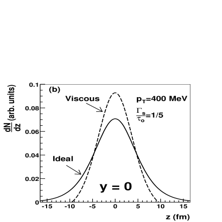
Figure 1: (a) The $p_{z}$ distribution of particles with coordinate-space rapidity $\eta_{s}=0$, with and without viscous corrections. (b) The $z$ distribution of particles with momentum-space rapidity $y=0$, with and without viscous corrections. The curves are drawn for a Bjorken expansion without transverse flow at $\tau_{o}=7\,\mbox{fm}$ for a Boltzmann gas with temperature, $T=160\,\mbox{MeV}$, $m=140\,\mbox{MeV}$. The transverse momentum is fixed, $p_{T}=400\,\mbox{MeV}$. The viscous correction is linearly proportional to $\Gamma_{s}/\tau_{o}$.

Due to boost invariance the $p_{z}$ distribution at $\eta_{s}=0$ is directly related to the $z$ distribution at $y=0$ GBaym . Specifically, for fixed transverse momentum, $\frac{dN}{dyd\eta_{s}}$ is a function of $\left|y-\eta_{s}\right|$, which leads to the relation

$$\left.m_{T}\frac{dN}{dp_{z}d\eta}\right|_{\eta=0}=\left.\tau_{o}\frac{dN}{dydz}\right|_{y=0}.$$ (19)

It follows that the z distribution at mid momentum-space rapidity is narrower as indicated in Fig. 1(b). The width of this z-distribution, is related to the longitudinal radius that is measured by HBT interferometry (see e.g. Wiedemann ).

To understand this result analytically we must calculate the width of z distribution for a simple Bjorken expansion of a Boltzmann gas at proper time $\tau_{o}$. Let us quickly recall the definitions of the HBT radii. The source function $S(x,K)$ for on shell pion emission is defined such that

$$E_{K}\frac{d^{3}N}{d^{3}K}\equiv\int d^{4}x\,S(x,K)$$ (20)

where $E_{K}=K^{0}=\sqrt{{\bf K}^{2}+m_{\pi}^{2}}$. Averages with respect to the source function are defined as $\left\langle\alpha\right\rangle_{\bf K}\equiv\int d^{4}x\,\alpha\,S(x,K)/\int d^{4}x\,S(x,K)$. To a good approximation (see e.g. Ref Wiedemann ), certain spatial and temporal variances of the source function can be determined from the Bose-Einstein correlations between pion pairs at small relative momenta. For a boost invariant and rotationally invariant source, we can assume without loss of generality that the pair momentum points in the x direction (i.e. ${\bf K}=(K^{x},K^{y},K^{z})=(K_{T},0,0)$). Then the following variances can be determined from HBT measurements

$$R_{O}^{2}(K_{T}) \equiv \left\langle(\tilde{x}-v_{K}\tilde{t})^{2}\right\rangle_{K_{T}}$$ (21)

$$R_{S}^{2}(K_{T}) \equiv \left\langle\tilde{y}^{2}\right\rangle_{K_{T}}$$ (22)

$$R_{L}^{2}(K_{T}) \equiv \left\langle\tilde{z}^{2}\right\rangle_{K_{T}}\;,$$ (23)

where $v_{K}=K_{T}/E_{K}$ and for example $\tilde{x}\equiv x-\langle x\rangle$. Comparing Eq. IV and Eq. 20, we see that in this work the source function is confined to a freezeout surface and therefore the averages are understood to mean

$$\left\langle\alpha\right\rangle_{\bf K}\equiv\frac{\int_{\Sigma}K^{\mu}\,d\Sigma_{\mu}\,\alpha\,f(x,K)}{\int_{\Sigma}K^{\mu}\,d\Sigma_{\mu}\,f(x,K)}\;.$$ (24)

The assumption of a sharp freezeout surface is clearly unrealistic. In general there is a transition region from hydrodynamics to the Knudsen limit. Within ideal hydrodynamics this transition region can not be determined. Within viscous hydrodynamics, viscous terms become large ($\sim 1/2$) and signal the transition.

Armed with these formula, the computation of $R_{L}^{2}$ for a boost invariant expansion is straight forward. We have

$$R_{L}^{2}(K_{T})\equiv\left\langle\tilde{z}^{2}\right\rangle_{K_{T}}\equiv\frac{\int K^{\mu}d\Sigma_{\mu}\,f(x,K)\,z^{2}}{\int K^{\mu}d\Sigma_{\mu}\,f(x,K)}\;.$$ (25)

Substituting $f=f_{o}+\delta f$, expanding to first order in $\delta f$, and performing the integrals (see Appendix B) we find the viscous correction $\delta R_{L}^{2}$

$$\frac{\delta R_{L}^{2}}{(R_{L}^{2})^{(0)}}=-\frac{\Gamma_{s}}{\tau_{o}}\left[\frac{6}{4}\frac{m_{T}}{T}\frac{K_{3}(\frac{m_{T}}{T})}{K_{2}(\frac{m_{T}}{T})}-\left(\frac{m_{T}}{T}\right)^{2}\frac{1}{8}\left(\frac{K_{3}(\frac{m_{T}}{T})}{K_{2}(\frac{m_{T}}{T})}-1\right)\right]\;,$$ (26)

where the $(R_{L}^{2})^{(0)}$ is the ideal longitudinal radius Bertsch

$$(R_{L}^{2})^{(0)}=\tau_{o}^{2}\frac{T}{m_{T}}\frac{K_{2}(x)}{K_{1}(x)}\;.$$ (27)

For the relevant range of $\frac{m_{T}}{T}$, the Bessel function expression in square brackets is large $\approx 6-8$. Accordingly, viscous corrections to the longitudinal radius are quite large ($>100\%$) and tend to reduce the radius relative to its ideal value. Including the transverse expansion reduces the viscous correction to $50\%$ . Nevertheless, the viscous correction to the longitudinal radius remains large unless $\Gamma_{s}/\tau_{o}$ is significantly smaller than $0.1$ . This formula and some caveats are discussed further in the next section.

V Viscous Corrections with Transverse Expansion

To go further and illustrate the effect of viscosity on the observed spectra, elliptic flow and HBT radii of hydrodynamical models of the heavy ion collision, I generalize the blast wave model to include the viscous corrections of Eq. 10. The blast wave model provides of a simple parametrization of the flow of full ideal hydrodynamic simulations which assume boost invariance Kolb1 ; Teaney1 . The corrections described below are therefore indicative of similar corrections to these simulations. This is the reason for adopting the blast wave model here. The blast wave model also has been used to fit experimental data. The model provides a good description of spectra and elliptic flow Kolb1 ; v2-star2 ; Jane and provides a fair description of HBT radii for small $M_{T}$, $M_{T}<0.5\,\mbox{GeV}$ StarQM2002 . However, for larger $M_{T}$ the model does not reproduce the strong dependence on $M_{T}$ seen in the $R_{O}$ and $R_{S}$ radii PhenixQM2002 ; Jane . The blast wave model remains simply a model of the flow fields and ultimately a full viscous simulation is needed to estimate viscous effects.

In the blast wave model of central collisions considered here, a hot pion gas is expanding in a boost invariant fashion and freezes out at a proper time $\tau_{o}$. In the transverse plane, the temperature is constant $T_{o}=160\,\mbox{MeV}$ and the matter distribution is uniform up to a radius $R_{o}$. The transverse velocity rises linearly as a function of the radius, $u^{r}=u^{o}\frac{r}{R_{O}}$. Summarizing, the hydrodynamic fields ($T$ and $u^{\mu}$) are parameterized as

$$T(\tau_{o},\eta_{s},r,\phi) = T_{o}\,\Theta(R_{o}-r)$$ (28a)

$$u^{r}(\tau_{o},\eta_{s},r,\phi) = u_{o}\frac{r}{R_{o}}\,\Theta(R_{o}-r)$$ (28b)

$$u^{\phi} = 0$$ (28c)

$$u^{\eta} = 0$$ (28d)

$$u^{\tau_{o}} = \sqrt{1+(u^{r})^{2}}\;.$$ (28e)

The blast wave parameters are adjusted so that model with the ideal thermal distribution can approximately reproduce the spectra and HBT radii. Similar blast wave model fits have appeared ubiquitously in the heavy ion literature (see e.g. Jane ). Then with the model parameters fixed, the viscous correction is calculated and compared to the ideal results. The model parameters for central collisions are recorded in Table 1.

	Central (0-5%)	Non-central (16-24%)
$T_{o}$ (MeV)	160	160
$R_{o}$ (fm)	10	7.5
$\tau_{o}$ (fm)	7.0	5.25
$u_{o}$	0.55	0.55
$u_{2}$	0	0.1

Table 1: Table of parameters used in the blast wave model described in the text.

With the hydrodynamic fields specified, the viscous tensor $\left\langle\nabla^{\alpha}u^{\beta}\right\rangle$ can be computed in a simple but lengthy calculation which is worked out in Appendix A. One technical point should be noted. In the viscous tensor $\left\langle\nabla^{\alpha}u^{\beta}\right\rangle$ time derivatives of the velocity appear. These time derivatives are converted into spatial derivatives using the ideal equations of motion which are sufficient to leading order in the viscosity.

The spectrum of particles emerging from the freezeout oriented 3-volume is calculated by employing the Cooper-Frye formula, Eq. 17. These integrals are performed numerically in a straightforward fashion. Again relevant details are relegated to Appendix A. The ideal spectrum of this blast wave model is typical of blast and is in rough agreement with pion data at RHIC. (See e.g. Jane for fits to data of this type.) In Fig. 2, the solid line shows the ratio of the viscous correction to the ideal spectrum. The dashed line shows the Bjorken result (Eq. 18) without transverse flow. The viscous correction becomes comparable to ideal results for $p_{T}\approx 1.7\,\mbox{GeV}$ indicating the breakdown of the hydrodynamic description of $p_{T}$ spectra for the flow profile considered here. Setting $\Gamma_{s}/\tau_{o}$ to $0.1$ extends the domain of applicability to $2.3\,\mbox{GeV}$. The analytic Bjorken result (Eq. IV) qualitatively explains the shape of Fig. 2. Quantitatively however, the transverse expansion alleviates some of the longitudinal shear and pushes the region of applicability hydrodynamics to somewhat larger transverse momentum.

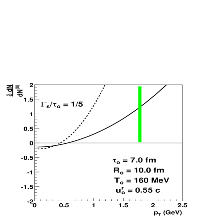
Figure 2: The solid line shows the ratio between the viscous correction ($\delta\,dN\equiv\frac{dN^{(1)}}{d^{2}p_{T}dy}$) and the ideal spectrum ($dN^{(0)}\equiv\frac{dN^{(0)}}{d^{2}p_{T}dy}$). The dashed line shows the Bjorken result without transverse flow given in Eq. 18. The band indicates where the hydrodynamic description of the $p_{T}$ spectrum in the blast wave model can not be reliably calculated. The viscous correction is linearly proportional to $\Gamma_{s}/\tau_{o}$.

Indeed, viscous effects are implicated in the heavy ion data for $p_{T}\approx 1.5\,\mbox{GeV}$. The observed elliptic flow deviates from ideal hydrodynamic results for $p_{T}\approx 1.5\,\mbox{GeV}$. Further for $p_{T}\approx 1.5\,\mbox{GeV}$, the single particle spectra start to deviate strongly from the hydrodynamic results (see e.g. Teaney1 ). Viscosity provides a simple explanation for the observed breakdown of the $p_{T}$ spectrum in this momentum range.

Next we examine the effect of viscosity on elliptic flow. In non-central collisions the radial velocity is given a small elliptic component to reproduce the observed elliptic flow

$$u^{r}(\tau_{o},\eta_{s},r,\phi) = u_{o}\frac{r}{R_{o}}(1+u_{2}\cos(2\phi))\,\Theta(R_{o}-r)\;.$$ (29)

The functional form of all other hydrodynamic fields is kept the same. Here we simulate the STAR 16-24% centrality bin which corresponds to an impact parameter bin $\langle b\rangle\approx 6.8\;\mbox{fm}$ v2-star1 . In the model, the radius and lifetime parameters ($R_{o}$ and $\tau_{o}$) are scaled downward from the central values by the ratio of the r.m.s. radii between $b=6.8\,\mbox{fm}$ and central AuAu collisions. This scaling of $R_{o}$ and $\tau_{o}$ approximates the impact parameter dependence of ideal hydrodynamic solutions Teaney1 . The non-central parameters are recorded in Table 1. As before, once the flow fields are specified, the viscous correction is found by differentiating $\left\langle\nabla^{\alpha}u^{\beta}\right\rangle$. The full form of the correction is given in Appendix A.

The elliptic flow as a function of transverse momentum $v_{2}(p_{T})$ is defined by Eq. 1. Expanding to first order

$$v_{2}(p_{T}) = v_{2}^{(0)}(p_{T})\left(1-\frac{\int d\phi\frac{d^{2}N^{(1)}}{p_{T}\,dp_{T}\,d\phi}}{\int d\phi\frac{d^{2}N^{(0)}}{p_{T}\,dp_{T}\,d\phi}}\right)+\frac{\int d\phi\cos(2\phi)\frac{d^{2}N^{(1)}}{p_{T}\,dp_{T}\,d\phi}}{\int d\phi\frac{d^{2}N^{(0)}}{p_{T}\,dp_{T}\,d\phi}}\;,$$ (30)

where $v_{2}^{(0)}(p_{T})$ denotes the elliptic flow as a function of $p_{T}$ calculated as in Eq. 1 but with the ideal distribution $\frac{dN^{(0)}}{p_{T}\,dp_{T}\,d\phi}$.

Fig. 3 shows the elliptic flow for pions. By construction,

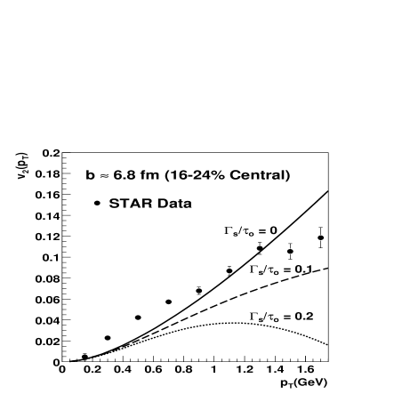
Figure 3: Elliptic flow $v_{2}$ as a function of $p_{T}$ for different values of $\Gamma_{s}/\tau_{o}$. The data points are four particle cummulant data from the STAR collaboration v2-star1 . Only statistical errors are shown. The difference between the ideal and viscous curves is linearly proportional to $\Gamma_{s}/\tau_{o}$.

the ideal curve $v_{2}^{(0)}$ roughly reproduces the experimental elliptic flow at $b\approx 6.8\,\mbox{fm}$. Taking a more realistic flow profile would improve the agreement of the ideal results with data Kolb1 . The effect of viscosity is to reduce the elliptic flow. Similar results were recently found Heinz-Wong by considering a partially thermalised expansion. Taken at face value these results suggest that the viscosity is small. Indeed, in order to agree with the ideal results up to $p_{T}\approx 1.0\,GeV$ we require $\Gamma_{s}/\tau_{o}\lesssim 0.1$ . It must be mentioned that the results of Fig. 3 are sensitive to the blast wave parameters. Ideal hydrodynamics generates an appropriate set of parameters. Whether a viscous expansion (with $\Gamma_{s}/\tau_{o}=0.1$) can reproduce the observed a elliptic flow remains an open question.

Finally, I discuss how viscosity effects HBT radii. First, I illustrate the ideal HBT radii for the blast wave parametrization in Fig. 4(a)

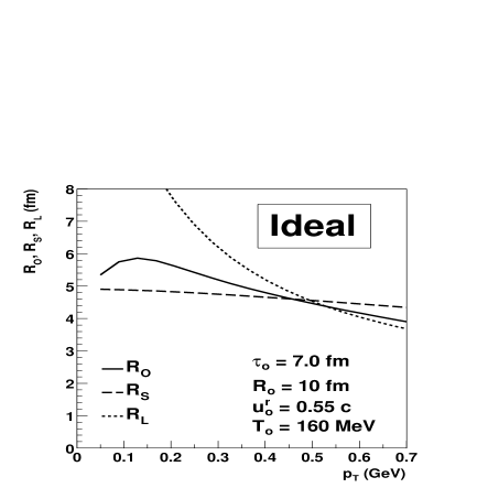
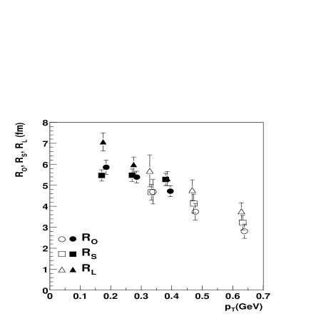
Figure 4: (a) Ideal blast wave fit to the experimental HBT radii $R_{O}$, $R_{S}$, and $R_{L}$ shown in (b) as a function of transverse momentum $K_{T}$. The solid symbols are from the STAR collaboration HBT-star and the open symbols are from the PHENIX collaboration HBT-phenix . For clarity, the experimental points have been slightly shifted horizontally.

The model parameters are again to chosen to approximately reproduce the observed radii which are illustrated in Fig. 4(b) for comparison. The viscous correction to each radius is again found by substituting $f=f_{o}+\delta f$ into Eq. 24 and expanding the numerator and denominator to first order in $\delta f$ and calculating the integrals numerically. The resulting viscous corrections are illustrated in Fig. 5.

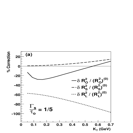
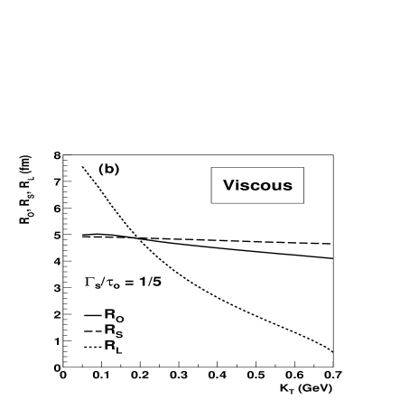
Figure 5: (a) Viscous correction $\delta R^{2}$ for $R_{O}$, $R_{S}$, and $R_{L}$ relative to ideal blast wave HBT radii $(R^{2})^{(0)}$ . (b) The HBT radii $R_{O}$, $R_{S}$, and $R_{L}$ including the viscous correction. The viscous correction is linearly proportional to $\Gamma_{s}/\tau_{o}$.

Several observations are immediate. First, as discussed in Sect. IV, the viscous corrections in the longitudinal directions reduce $\langle\tilde{z}^{2}\rangle$ and $\langle\tilde{t}^{2}\rangle$ due to the reduction of longitudinal pressure. This reduces the $R_{O}$ and $R_{L}$ radii. From a phenomenological point of view the reduction of $R_{L}$ is welcome In full ideal hydrodynamic simulations of heavy ion collisions assuming boost invariance in the longitudinal direction KolbHBT ; BassDumitru , $R_{L}$ is approximately twice too large compared to the data. In the blast wave model, viscous corrections to $R_{L}$ are large. This suggests that viscosity is responsible for the shortcomings in these simulations. Comparing Fig. 4(b) and Fig. 5(b), it seems that the reduction to $R_{L}$ is too large. However, it should be remembered that the parameters of the blast wave model have been adjusted to reproduce the ideal results and therefore viscous corrections make the agreement with data worse. Further, because the correction to the longitudinal radius is large the calculation can not be considered reliable. For $\Gamma_{s}/\tau_{o}\approx 0.1$ the viscous correction to $R_{L}$ is approximately $30-50\%$ and the calculation is more reliable.

Viscous corrections to the transverse variances $\langle\tilde{x}^{2}\rangle$ and $\langle\tilde{y}^{2}\rangle$ are small. Consequently, the sideward radius receives only a small viscous correction. Viscosity introduces no significant $x-t$ correlation which could influence the ratio of $R_{O}$ to $R_{S}$. In the blast wave model the difference between $R_{O}$ and $R_{S}$ is due to the contribution $\langle\tilde{t}^{2}\rangle$. Viscous corrections to $\langle\tilde{t}^{2}\rangle$ are negative and are essentially linearly proportional to this variance. For the particular value of $\Gamma_{s}/\tau_{o}=1/5$ the viscous correction is accidentally correct and makes $R_{O}/R_{S}\approx 1$ as illustrated in Fig. 5(b). The agreement is accidental but the trend is completely general. Viscosity reduces the $\langle\tilde{t}^{2}\rangle$ and therefore tends to make $R_{O}$ equal to $R_{S}$. This is also welcome from a phenomenological point of view. Full ideal hydrodynamic simulations (with KolbHBT ; BassDumitru and without Hirano the assumption of boost invariance) predict $R_{O}/R_{S}\approx 1.3$ which should be compared to $\sim 0.9$ observed in the RHIC data.

In spite of these welcome corrections, including viscosity makes some aspects of the hydrodynamic description of HBT radii worse. All of the observed radii (denoted generically as $R_{X}$) scale quite accurately with $m_{T}=\sqrt{K_{T}^{2}+m^{2}}$ as

$$R_{X}\propto\frac{1}{\sqrt{m_{T}}}\;.$$ (31)

Ideal hydrodynamics readily predicts this $\frac{1}{\sqrt{m_{T}}}$ scaling (see e.g. Sinyukov ; Csorgo1 ; Csorgo2 ). Indeed, expanding Eq. 27 for the longitudinal radius of an ideal boost invariant expansion, we obtain the Sinyukov-Makhlin formula Sinyukov

$$(R_{L}^{2})^{(0)}=\tau_{o}^{2}\frac{T}{m_{T}}\;.$$ (32)

Viscous terms immediately break this $\frac{1}{\sqrt{m_{T}}}$ scaling. Expanding Eq. 26 for the longitudinal radius with viscous corrections, we obtain

$$(R_{L}^{2})^{(0)}+\delta R_{L}^{2}=\tau_{o}^{2}\left(\frac{T}{m_{T}}-\frac{19}{16}\frac{\Gamma_{s}}{\tau_{o}}\right)\;.$$ (33)

Viscous terms break the ideal $\frac{1}{\sqrt{m_{T}}}$ scaling and this correction grows like $\frac{m_{T}}{T}$ relative to the ideal result. This deviation from $\frac{1}{\sqrt{m_{T}}}$ scaling is not seen in the data.

There remain several puzzling aspects in the HBT measurements for which viscosity offers no explanation. All of the radii are the same order of magnitude and fall with $m_{T}$ as in Eq. 31. In particular the steep fall with $m_{T}$ in the sideward radius was difficult to reproduce with the viscous blast wave model described here and in the ideal blast wave model Jane . This behavior was predicted based upon a parametrization of ideal hydrodynamics Csorgo1 ; Csorgo2 where system cools rapidly during freezeout and where temperature and velocity gradients are much larger than the geometric size of the system. It is natural to ask whether these conditions can be dynamically generated from some initial conditions or freezeout dynamics – see Csorgo3 for efforts in this direction. Large velocity gradients and temperature inhomogeneities should increase the relative importance of viscosity. Nevertheless, the success of these models should be noted.

VI Conclusions

In conclusion, I have calculated the first correction to the thermal distribution function of an expanding gas due to shear viscosity. The momentum range which is accurately described by hydrodynamics is directly related to the shear viscosity and depends upon the particular observable. I have estimated this momentum range for single particle spectra, elliptic flow, and HBT radii using the boost invariant blast wave model.

For reasonable values of $\Gamma_{s}\equiv\frac{4}{3}\frac{\eta}{e+p}$, the viscous correction to the single particle spectrum of a blast wave model becomes of order one for $p_{T}\approx 1.5-2.0\,\mbox{GeV}$ as illustrated Fig. 2.

The observed elliptic flow places a constraint on the shear viscosity. Indeed, unless $\Gamma_{s}/\tau_{o}$ is less than $0.1$, $v_{2}$ as a function of $p_{T}$ falls well below the ideal curve by $p_{T}\approx 1.0\,\mbox{GeV}$. For the blast wave model, the viscous corrections to elliptic observables become large $before$ the corresponding corrections to the transverse momentum spectra.

Shear viscosity also plays an important role in the interpretation of the longitudinal radius. Indeed, $R_{L}$ reflects not only the lifetime of the system but also the degree of thermalization in the longitudinal direction. $R_{L}$ involves the second moment of the thermal distribution function in the longitudinal direction where non-equilibrium effects are the largest. Consequently, viscous corrections to this radius (approximately 50% for $\Gamma_{s}/\tau_{o}\approx 0.2$ and 25% for $\Gamma_{s}/\tau_{o}\approx 0.1$ .) are large enough that perhaps $R_{L}$ should be left out of hydrodynamic fits to heavy ion data. This does not imply that hydrodynamics must be abandoned. On the contrary, while thermodynamics might accurately describe $\langle p_{T}\rangle$, it certainly does not accurately describe $\langle p_{T}^{100}\rangle$ unless the viscosity is very small. In addition, viscous corrections to the ideal longitudinal radius seem to contradict measurements of $R_{L}$. Shear corrections cause the longitudinal radius to deviate from the $\frac{1}{\sqrt{m_{T}}}$ scaling clearly seen in the data PhenixQM2002 ; Jane ; StarQM2002 and expected in ideal hydrodynamics Sinyukov .

Shear viscosity also reduces the ratio of $R_{O}$ to $R_{S}$ by decreasing the emission duration $\langle\tilde{t}\rangle$. Nevertheless, viscosity is not a panacea for the HBT problem. The sideward radius falls precipitously as a function of $K_{T}$. This precipitous fall can not be reproduced by hydrodynamics at least with a boost invariant expansion Csorgo . Viscous corrections to $R_{side}$ are small and make the sideward radius increase with $K_{T}$.

Many of the conclusions in this work about HBT radii were recently reached “from the opposite end” by Gyulassy and Molnar (GM) denes2 using kinetic theory. GM, started from the Knudsen limit, increased the transport opacity and increased the longitudinal radius. Here, I started from the ideal hydrodynamics, increased the viscosity and reduced of the longitudinal radius. These authors also emphasized the importance of the $y-\eta_{s}$ correlation in determining $R_{L}$. They also found only small viscous corrections to $R_{s}$ and experienced similar difficulties in reproducing the steep fall in $K_{T}$.

Clearly performing a full viscous calculation is the next step towards a complete thermodynamic description of the heavy ion reaction. Whether the shear viscosity can be made small enough ($\Gamma_{s}/\tau_{o}\lesssim 0.1$) in the early stages to reproduce the elliptic flow but still large enough ($\Gamma_{s}/\tau_{o}\approx 0.2$) in the late stages to reproduce $R_{L}$ and $R_{O}/R_{S}$ remains an open and important dynamical question.

Ackowledgements: I would like to thank Adrian Dumitru, Larry McLerran, Rob Pisarski, Edward Shuryak, and Raju Venugopalan for support. I would like to thank Denes Molnar for a careful reading of this manuscript. This work was supported by DE-AC02-98CH10886.

Appendix A The Viscous Tensor and Blast Wave Model

To write down the viscous tensor $\left\langle\nabla_{\alpha}u_{\beta}\right\rangle$ it is most convenient to use Bjorken coordinates: $\tau=\sqrt{t^{2}-z^{2}},\,\eta_{s}=\frac{1}{2}\log\left(\frac{t+z}{t-z}\right),\,r=\sqrt{x^{2}+y^{2}},$ and $\phi=\mbox{atan}\left(y/x\right)$. Note, we denote the space-time rapidity with $\eta_{s}$ and the viscous coefficient with $\eta$. However, we will drop the “s” on raised and lowered space-time indices when confusion can not arise. In this coordinate system the metric tensor is

$$g_{\mu\nu}=\bordermatrix{&\tau&\eta_{s}&r&\phi\cr\tau&1&0&0&0\cr\eta_{s}&0&-\tau^{2}&0&0\cr r&0&0&-1&0\cr\phi&0&0&0&-r^{2}\cr}$$ (34)

The only non-vanishing Christoffel symbols are $\Gamma^{\tau}_{\eta\eta}=\tau,\Gamma^{\eta}_{\tau\eta}=\frac{1}{\tau},\Gamma^{r}_{\phi\phi}=-r,\Gamma^{\phi}_{r\phi}=\frac{1}{r}$.

Without particle number conservation, the hydrodynamic fields are $T(\tau,\eta_{s},r,\phi)$ and $u^{\mu}(r,\eta_{s},r,\phi)$, where $\mu=r,\tau,\eta_{s},\phi$. The velocity field satisfies $u^{\mu}u_{\mu}=1$ and therefore only three components of $u^{\mu}$ need to be specified. For boost invariant flow $u^{\eta}=0$. For rotationally invariant flow $u^{\phi}=0$. For non-rotationally invariant flow we shall leave $u^{\phi}=0$ and leave the temperature profile rotationally invariant. We assume boost invariance throughout. By assumption, the particles freezeout at a proper time $\tau_{o}$ with a uniform distribution in the transverse plane and a linearly rising flow profile. Thus, the hydrodynamic fields are parameterized as

$$T(\tau_{o},\eta_{s},r,\phi) = T_{o}\,\Theta(R_{o}-r)$$ (35a)

$$u^{r}(\tau_{o},\eta_{s},r,\phi) = u_{o}\frac{r}{R_{o}}(1+u_{2}\cos(2\phi))\,\Theta(R_{o}-r)$$ (35b)

$$u^{\phi} = 0$$ (35c)

$$u^{\eta} = 0$$ (35d)

$$u^{\tau} = \sqrt{1+(u^{r})^{2}}\;.$$ (35e)

For central collisions $u_{2}$ is zero. It is useful to realize that $\tau u^{\eta}$ and $ru^{\phi}$ are the velocities in the $\eta$ and $\phi$ directions respectively.

The viscous tensor is constructed with the differential operator $\nabla^{\alpha}=\Delta^{\alpha\beta}d_{\beta}$, where $\Delta^{\alpha\beta}$ denotes the projector, $g^{\alpha\beta}-u^{\alpha}u^{\beta}$, and $d_{\beta}$ denotes the the covariant derivative, $d_{\beta}u^{\alpha}=\partial_{\beta}u^{\alpha}+\Gamma^{\alpha}_{\mu\beta}u^{\mu}$. With these definitions the viscous tensor is given by $\eta\left\langle\nabla_{\alpha}u_{\beta}\right\rangle$, where $\left\langle\nabla_{\alpha}u_{\beta}\right\rangle\equiv\nabla_{\alpha}u_{\beta}+\nabla_{\beta}u_{\alpha}-\frac{2}{3}\Delta_{\alpha\beta}\nabla_{\gamma}u^{\gamma}$. Assuming boost invariance, the spatial components of the viscous tensor are given by

$$r\left\langle\nabla^{r}u^{\phi}\right\rangle = -r\partial_{r}u^{\phi}-\frac{1}{r}\partial_{\phi}{u^{r}}-ru^{r}Du^{\phi}-ru^{\phi}Du^{r}-\frac{2}{3}r\Delta^{r\phi}\frac{1}{\sqrt{-g}}\partial_{\mu}(\sqrt{-g}u^{\mu})$$ (36a)

$$r^{2}\left\langle\nabla^{\phi}u^{\phi}\right\rangle = -2\partial_{\phi}u^{\phi}-2\frac{u^{r}}{r}-2r^{2}u^{\phi}Du^{\phi}-\frac{2}{3}r^{2}\Delta^{\phi\phi}\frac{1}{\sqrt{-g}}\partial_{\mu}(\sqrt{-g}u^{\mu})$$ (36b)

$$\left\langle\nabla^{r}u^{r}\right\rangle = -2\partial_{r}u^{r}-2u^{r}Du^{r}-\frac{2}{3}\Delta^{rr}\frac{1}{\sqrt{-g}}\partial_{\mu}(\sqrt{-g}u^{\mu})$$ (36c)

$$\tau^{2}\left\langle\nabla^{\eta}u^{\eta}\right\rangle = -2\frac{u^{\tau}}{\tau}+\frac{2}{3}\frac{1}{\sqrt{-g}}\partial_{\mu}(\sqrt{-g}u^{\mu})$$ (36d)

$$\left\langle\nabla^{r}u^{\eta}\right\rangle = \left\langle\nabla^{\phi}u^{\eta}\right\rangle=0\;.$$ (36e)

Here $\sqrt{-g}=\tau r$, the expansion scalar is given by

$$\frac{1}{\sqrt{-g}}\partial_{\mu}(\sqrt{-g}u^{\mu})=\frac{u^{\tau}}{\tau}+\frac{u^{r}}{r}+\partial_{\phi}u^{\phi}+\partial_{r}u^{r}+\partial_{\tau}u^{\tau},$$ (37)

and the time derivatives in the rest frame $Du^{\mu}=u^{\alpha}d_{\alpha}u^{\mu}$ are given by

$$Du^{r} = u^{\tau}\partial_{\tau}u^{r}+u^{r}\partial_{r}u^{r}+u^{\phi}\partial_{\phi}u^{r}-r(u^{\phi})^{2}$$ (38)

$$rDu^{\phi} = u^{\tau}\partial_{\tau}(ru^{\phi})+u^{r}\partial_{r}(ru^{\phi})+u^{\phi}\partial_{\phi}(ru^{\phi})+u^{\phi}u^{r}\;.$$ (39)

Once the spatial components of the viscous stress energy tensor are known the temporal components are determined (numerically) from the relations, $\left\langle\nabla^{\alpha}u^{\beta}\right\rangle u_{\beta}=0$.

In these equations the time derivatives, $\partial_{\tau}u^{\phi},\partial_{\tau}u^{r}$, and $\partial_{\tau}u^{\tau}$ appear. To fix the value of these time derivatives it is sufficient to consider the ideal equations of motion. Inclusion of viscous terms would lead to previously neglected second order corrections in $\frac{\Gamma_{s}}{\tau}$. The ideal equations of motion can be written

$$De = -(e+p)\,\nabla_{\mu}u^{\mu}$$ (40)

$$Du^{\mu} = +\frac{\nabla^{\mu}p}{e+p}\;.$$ (41)

With these two equations for $De$ and $Du^{r}$, and the flow profile given in Eqs. 35, the time derivatives can be determined

$$\partial_{\tau}u^{\phi} = 0$$ (42a)

$$\partial_{\tau}u^{r} = \frac{c_{s}^{2}v}{1-c_{s}^{2}v^{2}}\left(\frac{u^{\tau}}{\tau}+\frac{u^{r}}{r}+\partial_{r}u^{r}+v^{2}\partial_{r}u^{r}\right)-v\partial_{r}u^{r}$$ (42b)

$$\partial_{\tau}u^{\tau} = v\partial_{\tau}u^{r}\;.$$ (42c)

Here $v=u^{r}/u^{\tau}$ is the radial velocity and $c_{s}^{2}=\frac{dp}{de}$ denotes the squared speed of sound. $c_{s}^{2}$ is very close to $\frac{1}{3}$ for the pion gas considered and is found by differentiating the equation of state for a single component massive classical ideal gas. See e.g. Raju for explicit formulas for the pressure and energy density. With the necessary time derivatives, the full viscous tensor can be found by substituting the flow profile given in Eq. 35 into Eq. 36 and differentiating. The final formulas are lengthy and are not given. A check of the algebra is provided by the trace relation, $g_{\mu\nu}T_{vis}^{\mu\nu}=0$.

An additional prescription for fixing the time derivative was tried. If the particles are freezing out, then the particles are free streaming. Accordingly, we have $Du^{\mu}=0$. This amounts to dropping terms proportional to $c_{s}^{2}$ when computing Eq. 42. This change made only a negligible change to final results. This is because the whole effect of the time derivative is proportional to $c_{s}^{2}v^{2}$ which is rather small in practice, $c_{s}^{2}v^{2}\approx\frac{1}{10}$.

To finish computing the viscous correction $p^{\mu}p^{\nu}\langle\nabla_{\mu}u_{\nu}\rangle$ we need to express $p^{\mu}$ and the integration measure $p^{\mu}d\Sigma_{\mu}$ in the ($\tau,\eta_{s},r,\phi$) coordinate system. For a particle at point $(\tau,\eta_{s},r,\phi)$ with four momentum $p^{\mu}=(E,p^{x},p^{y},p^{z})=(m_{T}\cosh y,p_{T}\cos\phi_{p},p_{T}\sin\phi_{p},m_{T}\sinh y)$ we have

$$p^{\tau} = m_{T}\cosh(y-\eta_{s})$$ (43a)

$$\tau p^{\eta} = m_{T}\sinh(y-\eta_{s})$$ (43b)

$$p^{r} = p_{T}\cos(\phi_{p}-\phi)$$ (43c)

$$rp^{\phi} = p_{T}\sin(\phi_{p}-\phi)\;.$$ (43d)

The oriented freezeout volume is $d\Sigma_{\mu}=(d\Sigma_{\tau},d\Sigma_{r},d\Sigma_{\phi},d\Sigma_{\eta})=(\tau d\eta_{s}\,rdr\,d\phi,0,0,0)$ and the integration measure is

$$p^{\mu}d\Sigma_{\mu} = m_{T}\cosh(y-\eta_{s})\,\tau d\eta_{s}\,rdr\,d\phi\;.$$ (44)

With these formulas there is ample information to compute the viscous correction $p^{\mu}p^{\nu}\langle\nabla_{\mu}u_{\nu}\rangle$ and to perform the necessary Cooper-Frye integrals.

Appendix B Viscous Corrections to a Bjorken expansion

In this appendix I provide the details leading to the viscous corrections to the spectrum and longitudinal radius (Eqs. IV and 26) for a boost invariant expansion without transverse flow. The spectrum is given by the Cooper-Frye formula, Eq. 17. First we compute the ideal spectrum. For a boost invariant expansion without a transverse flow $u^{\tau}=1$ and $u^{\eta}=u^{r}=u^{\phi}=0$. The thermal distribution for an expanding Boltzmann gas is $f_{o}\left(\frac{p\cdot u}{T}\right)=\exp\left(-\frac{m_{T}\cosh(y-\eta_{s})}{T}\right)$. Then the Cooper-Frye integral gives the thermal spectrum from an expanding cylinder

$$\frac{d^{2}N^{(0)}}{d^{2}p_{T}\,dy} = \frac{1}{(2\pi)^{3}}\int p^{\mu}d\Sigma_{\mu}\,f_{o}\left(\frac{p\cdot u}{T}\right)$$ (45)

Substituting the integration measure $p^{\mu}d\Sigma_{\mu}$ we have

$$\frac{d^{2}N^{(0)}}{d^{2}p_{T}\,dy} = \frac{1}{(2\pi)^{3}}\int_{0}^{R_{o}}r\,dr\,\int_{0}^{2\pi}d\phi\int_{-\infty}^{\infty}\tau\,d\eta_{s}\,m_{T}\cosh(y-\eta_{s})\,f_{o}(\frac{p\cdot u}{T})\;.$$ (46)

Performing the integral we obtain the ideal thermal spectrum

$$\frac{d^{2}N^{(0)}}{d^{2}p_{T}\,dy} = m_{T}\tau_{o}\,\frac{\pi R_{o}^{2}}{(2\pi)^{3}}\,2K_{1}(x)\;.$$ (47)

Here $K_{1}(x)$ is the modified Bessel function evaluated at $x\equiv\frac{m_{T}}{T}$. Now we determine the correction spectrum. For a pure boost invariant expansion the non-vanishing components of viscous tensor $\left\langle\nabla^{\mu}u^{\nu}\right\rangle$ are from Eqs. 36

$$\left\langle\nabla^{r}u^{r}\right\rangle = \frac{2}{3\tau}$$ (48a)

$$r^{2}\left\langle\nabla^{\phi}u^{\phi}\right\rangle = \frac{2}{3\tau}$$ (48b)

$$\tau^{2}\left\langle\nabla^{\eta}u^{\eta}\right\rangle = -\frac{4}{3\tau}\;.$$ (48c)

Thus the viscous correction $\delta f$ is

$$\delta f=\frac{3}{8}\frac{\Gamma_{s}}{T^{2}}\,f_{o}\left(\frac{p\cdot u}{T}\right)p^{\mu}p^{\nu}\,\left\langle\nabla_{\mu}u_{\nu}\right\rangle = \frac{3}{8}\frac{\Gamma_{s}}{T^{2}}\,f_{o}\left(\frac{p\cdot u}{T}\right)\left(\frac{2\,p_{T}^{2}}{3\tau}-\frac{4m_{T}^{2}}{3\tau}\sinh^{2}\eta_{s}\right)$$ (49)

Note we have substituted $f_{o}(1+f_{o})$ in Eq. III by $f_{o}$ as required by the Boltzmann approximation. We can then substitute $\delta f$ to determine the first viscous correction

$$\frac{d^{2}N^{(1)}}{d^{2}p_{T}\,dy} = \frac{1}{(2\pi)^{3}}\int p^{\mu}d\Sigma_{\mu}\delta f\;.$$ (50)

Substituting the integration measure and performing the integral over the $\eta_{s}$ as for the ideal case we obtain

$$\frac{d^{2}N^{(1)}}{d^{2}p_{T}\,dy} = m_{T}\tau_{o}\,\frac{\pi R_{o}^{2}}{(2\pi)^{3}}\,2K_{1}(x)\,\frac{\Gamma_{s}}{4\tau}\left(\left(\frac{p_{T}}{T}\right)^{2}-\left(\frac{m_{T}}{T}\right)^{2}\left(\frac{K_{3}(x)}{K_{1}(x)}-1\right)\right)\;.$$ (51)

Dividing Eq. 51 with Eq. 47 we obtain Eq. IV given the text.

Next we work out the first viscous correction to the longitudinal HBT radius. The longitudinal radius is given by Eq. 25. Expanding to first order in $\delta f$ and using the relation $z=\tau_{o}\sinh\eta_{s}$ we obtain the ideal contribution

$$(R_{L}^{2})^{(0)}(K_{T}) = \frac{\int K^{\mu}d\Sigma_{\mu}\,f_{o}(\frac{K\cdot u}{T})\,\tau_{o}^{2}\sinh^{2}\eta_{s}}{\int K^{\mu}d\Sigma_{\mu}\,f_{o}(\frac{K\cdot u}{T})\;,}$$ (52)

and the first viscous correction

$$\delta R_{L}^{2}(K_{T}) = (R_{L}^{2})^{(0)}\left(\frac{\frac{dN^{(1)}}{K_{T}dK_{T}}}{\frac{dN^{(0)}}{K_{T}dK_{T}}}\right)+\frac{\int K^{\mu}d\Sigma_{\mu}\,\delta f\tau_{o}^{2}\sinh^{2}\eta_{s}}{\int K^{\mu}d\Sigma_{\mu}\,f_{o}(\frac{K\cdot u}{T})}\;.$$ (53)

For the kinematics of typical HBT measurements at mid rapidity, we have $K^{\mu}=(K^{\tau},K^{r},K^{\phi},K^{\eta})=(\sqrt{K_{T}^{2}+m^{2}},K_{T},0,0)$ . The integration measure is $K^{\mu}d\Sigma_{\mu}=m_{T}\cosh(\eta_{s})\,\tau\,d\eta_{s}\,rdr\,d\phi$ where $m_{T}=\sqrt{K_{T}^{2}+m^{2}}$.

First we work out the ideal radius, $(R_{L}^{2})^{(0)}$. Substituting $K^{\mu}d\Sigma_{\mu}$ into the numerator and denominator and performing the integrals over the freezeout surface (as in Eq. 46) we obtain the Herrmann-Bertsch formula Bertsch

$$(R_{L}^{2})^{(0)}=\tau_{o}^{2}\frac{T}{m_{T}}\frac{K_{2}(x)}{K_{1}(x)}\;,$$ (54)

where $x\equiv\sqrt{m^{2}+K_{T}^{2}}/T$. For large values of $x$, Eq. 54 reduces to the Makhlin-Sinyukov formula Sinyukov

$$(R_{L}^{2})^{(0)}=\tau_{o}^{2}\frac{T}{m_{T}}\;.$$ (55)

A similar calculation gives the viscous correction. Substituting the viscous correction $\delta f$ (Eq. 49) into Eq. 53, using the previous results for the spectrum (Eqs. 47, 51) and ideal radius (Eq. 54), and performing the $\eta_{s}$ integrals, we obtain Eq.  26 quoted in the text

$$\frac{\delta R_{L}^{2}}{(R_{L}^{2})^{(0)}} = -\frac{\Gamma_{s}}{\tau}\left(\frac{6}{4}\frac{xK_{3}(x)}{K_{2}(x)}-x^{2}\frac{1}{8}\left(\frac{K_{3}(x)}{K_{2}(x)}-1\right)\right)\;.$$ (56)

References

(1)
K. H. Ackermann et al., (STAR Collaboration),
Phys. Rev. Lett. 86, 402 (2001).
(2)
C. Adler et al. (STAR Collaboration),
Phys. Rev. Lett. 87, 03490 (2002).
(3)
C. Adler et al. (STAR Collaboration),
Phys. Rev. C 66, 03490 (2002).
(4)
K. Adcox et al. (PHENIX Collaboration),
Phys. Rev. Lett. 89, 212301 (2002).
(5)
B. B. Back et al. (PHOBOS Collaboration),
Phys. Rev. Lett. 89, 222301 (2002).
(6)
D. Molnar and M. Gyulassy,
Nucl. Phys. A 697, 495 (2002).
(7)
G. Policastro, D. T. Son, A. 0. Starinets,
Phys. Rev. Lett. 87, 081601 (2001) ;
JHEP 0209, 043 (2002);
hep-th/0210220.
(8)
D. Teaney, J. Lauret, and E.V. Shuryak,
Phys. Rev. Lett. 86, 4783 (2001);
D. Teaney, J. Lauret, and E.V. Shuryak, nucl-th/0110037.
(9)
P.F. Kolb, P.Huovinen, U. Heinz, H. Heiselberg,
Phys. Lett. B 500, 232 (2001);
P. Huovinen, P.F. Kolb, U. Heinz, H. Heiselberg,
Phys. Lett. B 503, 58 (2001).
(10)
S. Soff, S. A. Bass, Adrian Dumitru,
Phys. Rev. Lett. 86, 3981 (2001).
(11)
C. Adler et al. (STAR Collaboration),
Phys. Rev. Lett 87, 082301 (2001).
(12)
K. Adcox et al. (PHENIX Collaboration),
Phys. Rev. Lett. 88, 192302 (2002).
(13)
A. Dumitru, nucl-th/0206011.
(14)
R. C. Hwa, Phys. Rev. D. 10, 2260 (1974).
(15)
J. D. Bjorken, Phys. Rev. D. 27, 140 (1983).
(16)
G. Baym, Phys. Lett. B 138, 18 (1984).
(17)
P. Danielewicz, M. Gyulassy,
Phys. Rev. D 31, 53 (1985).
(18)
M. Prakash, M. Prakash, R. Venugopalan, G. Welke,
Phys. Rept. 227, 327 (1993).
(19)
Peter Arnold, Guy D. Moore, Laurence G. Yaffe,
JHEP 0011, 001 (2000).
(20)
G. Baym, H. Monien, C. J. Pethick and D. G. Ravenhall,
Phys. Rev. Lett. 64, 1867 (1990).
(21)
S. S. Gubser, I. R. Klebanov, A. A. Tseytlin,
Nucl. Phys. B 534, 202 (1998).
(22)
S. Weinberg, Astrophysical J. 168, 175 (1971) .
(23)
A. J. Kox, S. R. de Groot, and W.A. Van Leeuwen,
Physica 84 A, 155 (1976).
(24)
S. de Groot, W. van Leeuven, Ch. van Veert,
Relativistic Kinetic Theory (North-Holland, 1980).
(25)
R. Venugopalan and M. Prakash,
Nucl. Phys. A 546, 718 (1992). Appendix A.
(26)
F. Cooper and G. Frye,
Phys. Rev. D. 10, 186 (1974) .
(27)
U. Wiedemann and U. Heinz, Phys. Rept. 319, 145 (1999).
(28)
M. Herrmann and G. F. Bertsch,
Phys. Rev. C 51, 328 (1995).
(29)
J. M. Burward-Hoy, for the PHENIX Collaboration, in Quark Matter 2002,
Nucl. Phys. A 715, 498c (2003).
(30)
M. Lopéz Noriega, for the STAR Collaboration, in Quark Matter 2002,
Nucl. Phys. A 715, 623c (2003).
(31)
A. Enokizono, for the PHENIX Collaboration, in Quark Matter 2002,
Nucl. Phys. A 715, 595c (2003).
(32)
U. Heinz and S.M.H. Wong
Phys. Rev. C 66, 014907 (2002).
(33)
U. Heinz and P.F. Kolb, Phys. Lett. B 542, 216 (2002).
(34)
T. Hirano and K. Tsuda, Phys. Rev. C 66, 054905 (2002).
(35)
A. N. Makhlin, Yu. M. Sinyukov,
Z. Phys. C 39, 69 (1988).
(36)
T. Csörgő and B. Lorstad, Phys. Rev. C 54, 1390 (1996).
(37)
T. Csörgő and B. Lorstad, Nucl. Phys. A 590, 465 (1995).
(38)
T. Csörgő, F. Grassi, Y. Hama, and T. Kodama, hep-ph/0204300;
ibid., hep-ph/0203204.
(39)
T. Csörgő and A. Ster, nucl-th/0207016.
(40)
D. Molnar and M. Gyulassy,
nucl-th/0211017.