Nuclear Wave Functions for Spin and Pseudospin Partners

Abstract

Using relations between wave functions obtained in the framework of the relativistic mean field theory, we investigate the effects of pseudospin and spin symmetry breaking on the single nucleon wave functions in spherical nuclei. In our analysis, we apply both relativistic and non-relativistic self-consistent models as well as the harmonic oscillator model.

I Introduction

Pseudospin symmetry was suggested in the late sixties [Hec69] ; [Ari69] based on the small energy difference between nuclear energy levels with quantum numbers (n,$\ell$,j=$\ell$+1/2) and (n-1,$\ell$+2,j=$\ell$+3/2). Pseudospin coupling schemes were observed and used to explain different aspects of nuclear structure [Jon71] ; [Bak72] ; [Str72] ; [Rat73] . In particular, pseudospin symmetry was considered in the context of deformation [Boh82] and superdeformation [Dud87] , magnetic moment interpretation [Tro94] ; [Stu99] ; [Stu02] and identical bands [Naz90a] ; [Ste90] . However, the origin of this symmetry was unknown. It was noticed that, in the relativistic mean field (RMF) calculations, energy differences between pseudospin partners were small [Blo95] , but it was not until 1997 when the origin of this phenomenon was understood [Gin97] in terms of near-equility of the absolute values of scalar $V_{S}(\bf r)$ and vector $V_{V}(\bf r)$ potentials [Coh91] . This observation stimulated a number of works on this subject [Gin98a] ; [Gin98] ; [Men98b] ; [Sug98] ; [Gin99a] ; [Gin99] ; [Men99] ; [Sug02] ; [Gin00a] ; [Gin01] ; [Gin01a] ; [Gin02] .

Although the origin of pseudospin symmetry has been explained, it is still an open question why this symmetry is obeyed so well in non-relativistic calculations. This question is particularly important for superheavy nuclei and nuclei far from stability where shell effects are crucial and a subtle change in interaction may effect even in changing magic numbers (see, e.g., discussion in Ref. [Kru00] ).

Although spin symmetry appears to be broken since spin-orbit splittings are very large, it is possible that the spin symmetry breaking may be a dynamic symmetry, i.e., the energy levels are not degenerate but the eignefunctions preserve the symmetry. In this paper we, therefore, compare effects of both pseudospin and spin symmetry breaking for non-relativistic as well as relativistic single-nucleon eigenfunctions for spherical nuclei.

The structure of the paper is the following. In Sec. II, we briefly introduce the main pseudospin relations consistent with the Dirac equation. Numerical evidences for pseudospin dynamic symmetry in nuclei are analyzed in Sec. III, while the Sec. IV is devoted to the spin symmetry. Calculations have been performed for a number of spherical doubly-magic nuclei. The results presented in this paper correspond to ²⁰⁸Pb, as a representative case. Conclusions are presented in Sec. V.

II Pseudospin symmetry and the Dirac Hamiltonian

II.1 Pseudospin Conditions on the Dirac Hamiltonian

The Dirac Hamiltonian ($\hbar=c=1$)

$$H=\bm{\alpha}\cdot{\bf p}+V_{V}({\bf r})+\beta V_{S}({\bf r})+\beta\ M.$$ (1)

with external scalar $V_{S}(\bf{r})$ and vector $V_{V}({\bf r})$ potentials, vanishing space components and non-vanishing time component, is invariant under an SU(2) algebra if the scalar potential $V_{S}({\bf r})$ and the vector potential $V_{V}({\bf r})$ are related up to a constant $C_{ps}$ [Bel75] ; [Gin97] :

$$V_{S}({\bf r})+V_{V}({\bf r})=C_{ps}.$$ (2)

The pseudospin generators

$${\bf{\tilde{S}}}=\left(\begin{array}[]{cc}{\bf{\tilde{s}}}&0\\ 0&{\bf{s}}\end{array}\right)$$ (3)

form an SU(2) algebra

$$[{\tilde{S}}_{i},{\tilde{S}}_{j}]=i\epsilon_{ijk}\ {\tilde{S}}_{k},$$ (4)

where ${\bf{\tilde{s}}}=U_{p}\ {\bf{s}}\ U_{p}~{}$, $U_{p}=\bm{\sigma}\cdot\hat{\bf{p}}$ is the helicity transformation [Blo95] , ${\bf s}=\bm{\sigma}/2$, and ${\sigma_{i}}~{}$ are the usual Pauli matrices.

The operators ${\tilde{S}}_{i}$ commute with the Dirac Hamiltonian $H_{ps}$ satisfying conditions (2):

$$[{\tilde{S}}_{i},H_{ps}]=0,$$ (5)

thus generating an SU(2) invariant symmetry of $H_{ps}$.

II.2 Pseudospin Conditions on the Dirac Eigenfunctions

According to the SU(2) invariant symmetry of $H_{ps}$, each eigenstate of the Dirac Hamiltonian $H_{ps}$ with the third component of pseudospin ${\tilde{\mu}}={1\over 2}$ has a partner with ${\tilde{\mu}}=-{1\over 2}$ and the same energy, i.e.,

$$H_{ps}\ \Phi_{k{\tilde{\mu}}}^{ps}({\bf r})=E_{k}\Phi_{k{\tilde{\mu}}}^{ps}({\bf r})$$ (6)

where ${\tilde{\mu}}=\pm{1\over 2}$ is the eigenvalue of ${\tilde{S}}_{z}$,

$${\tilde{S}}_{z}\ \Phi_{k{\tilde{\mu}}}^{ps}({\bf r})={\tilde{\mu}}\ \Phi_{k{\tilde{\mu}}}^{ps}({\bf r}),$$ (7)

and $k$ are the other quantum numbers. The eigenstates in the doublet are connected by the generators ${\tilde{S}}_{\pm}~{}$:

$${\tilde{S}}_{\pm}\ \Phi_{k{\tilde{\mu}}}^{ps}({\bf r})=\sqrt{{\left({1\over 2}\mp{\tilde{\mu}}\right)\left({3\over 2}\pm{\tilde{\mu}}\right)}}\ \Phi_{k{\tilde{\mu}}\pm 1}^{ps}({\bf r}).$$ (8)

The generators (7), (8) do not mix upper and lower components of the Dirac eigenfunctions $\Phi_{k{\tilde{\mu}}}^{ps}({\bf r})$. Since the spin operates on the lower components only (see Eq. (3)), one of predictions of this symmetry is that the spatial amplitudes of the lower components of the Dirac wave functions are identical in shape [Gin98] . For spherical nuclei this means that the lower components of the pseudospin doublets have the same radial quantum number ${\tilde{n}}=n$ [Gin01a] and the same spherical harmonic rank ${\tilde{\ell}}=\ell+1$. Therefore, it is natural to label the doublets with their pseudospin quantum numbers $({\tilde{n}},{\tilde{\ell}},j={\tilde{\ell}}\pm{1\over 2})$. The Dirac eigenfunctions then have the form

$$\Phi^{ps}_{{\tilde{n}},{\tilde{\ell}},j,m}({\bf r})=\ \left(\begin{array}[]{c}g_{{\tilde{n}}{\tilde{\ell}}j}(r)\ [Y^{({\tilde{\ell}}_{j})}(\theta,\phi)\ \chi]^{(j)}_{m}\\ if_{{\tilde{n}}{\tilde{\ell}}}(r)\ [Y^{({\tilde{\ell}})}(\theta,\phi)\ \chi]^{(j)}_{m}\end{array}\right).$$ (9)

where $\chi_{\mu}$ is the spin function, $Y^{({\tilde{\ell}})}(\theta,\phi)$ is the spherical harmonic of rank ${\tilde{\ell}}$, and ${\tilde{\ell}}_{j}={\tilde{\ell}}\pm 1$ for $j={\tilde{\ell}}\pm{1\over 2}$

As stated above, the radial wave functions of the lower components are equal:

$$f_{{\tilde{n}}{\tilde{\ell}}j={\tilde{\ell}}-{1\over 2}}(r)=f_{{\tilde{n}}{\tilde{\ell}}j={\tilde{\ell}}+{1\over 2}}(r).$$ (10)

On the other hand, the generators for the upper components depend on the momentum as well as the spin so they intertwine spin and space. Therefore, in the pseudospin symmetry limit, the radial wave functions of the upper components $g_{{\tilde{n}}{\tilde{\ell}}j={\tilde{\ell}}\pm{1\over 2}}(r)$ satisfy differential relations [Gin02] :

$$D_{{\tilde{n}}{\tilde{\ell}}j={\tilde{\ell}}-{1\over 2}}(r)\ g_{{\tilde{n}}{\tilde{\ell}}j={\tilde{\ell}}-{1\over 2}}(r)={}$$ (11)

$${}=D_{\tilde{n}\tilde{\ell}j={\tilde{\ell}}+{1\over 2}}(r)g_{{\tilde{n}}{\tilde{\ell}}j={\tilde{\ell}}+{1\over 2}}(r),$$

where

$$\begin{array}[]{lll}D_{{\tilde{n}}{\tilde{\ell}}j={\tilde{\ell}}-{1\over 2}}(r)&=&\left(\frac{d}{dr}-\frac{{\tilde{\ell}}-1}{r}\right),\\ \\ D_{{\tilde{n}}{\tilde{\ell}}j={\tilde{\ell}}+{1\over 2}}(r)&=&\left(\frac{d}{dr}+\frac{{\tilde{\ell}}+2}{r}\right).\end{array}$$ (12)

In the non-relativistic limit, $g_{{\tilde{n}}{\tilde{\ell}}j}(r)$ is associated with the single particle wave function while $f_{{\tilde{n}}{\tilde{\ell}}j}(r)$ vanishes. Relativistic mean field calculations show that indeed $f_{{\tilde{n}}{\tilde{\ell}}j}(r)$ is small compared to $D_{{\tilde{n}}{\tilde{\ell}}j}g_{{\tilde{n}}{\tilde{\ell}}j}(r)$. The factor is roughly six as we shall see below.

II.3 Dirac Conditions on the Pseudospin Doublet States

Pseudospin symmetry relates upper components in the doublets to each other and lower components to each other, but pseudospin symmetry does not relate upper components to lower components because the pseudospin generators (3) are diagonal. It is, of course, the Dirac equation, which relates upper to lower components.

For spherically symmetric potentials, the Dirac equation is reduced to coupled first order differential equations in the radial coordinate only leading to [Gin97]

$$D_{\tilde{n}\tilde{\ell}j}(r)g_{\tilde{n}\tilde{\ell}j}(r)={}$$ (13)

$${}=\left[2M+V_{S}(r)-V_{V}(r)-E\right]f_{\tilde{n}\tilde{\ell}j}(r),$$

$$D_{n{\ell}j}(r)f_{{n}{\ell}j}(r)={}$$ (14)

$${}=\left[V_{S}(r)+V_{V}(r)+E\right]g_{{n}{\ell}j}(r),$$

where $V_{S}(r)$ and $V_{V}(r)$ are spherical potentials and $E$ is the binding energy.

For heavy nuclei, the vector and scalar potentials are approximately constant inside the nuclear interior. At the nuclear surface the potentials fall rapidly to zero and hence outside the nuclear surface both $f(r)$ and $g(r)$ decrease exponentially. Also the nucleon mass is very large compared to the binding energy. In the nuclear interior $V_{S}(r)-V_{V}(r)\approx$const, hence

$$D_{{\tilde{n}}{\tilde{\ell}}j}(r)g_{{\tilde{n}}{\tilde{\ell}}j}(r)\approx\ \lambda\ f_{{\tilde{n}}{\tilde{\ell}}j}(r),$$ (15)

where $\lambda=2M+V_{S}(r)-V_{V}(r)-E\approx 6$ fm^-1 in our calculations. Notice that in the pseudospin symmetry limit $f_{{\tilde{n}}{\tilde{\ell}}j}(r)=f_{{\tilde{n}}{\tilde{\ell}}}(r)$ and, therefore, Eqs. (13), (14) are consistent with Eq. (11).

III Pseudospin Dynamic Symmetries

The relation (11) is strictly fulfilled only under condition (2), $V_{S}+V_{V}=C_{ps}$, [Gin02] . Therefore, comparing the differences between $D_{{\tilde{n}}{\tilde{\ell}}j={\tilde{\ell}}-{1\over 2}}(r)g_{{\tilde{n}}{\tilde{\ell}}j={\tilde{\ell}}-{1\over 2}}(r)$ and $D_{{\tilde{n}}{\tilde{\ell}}j={\tilde{\ell}}+{1\over 2}}(r)g_{{\tilde{n}}{\tilde{\ell}}j={\tilde{\ell}}+{1\over 2}}(r)$, one can learn about the pseudospin symmetry breaking effects. The differential relations (11) have been checked previously only for the RMF approximation of a relativistic Lagrangian with zero range interactions [Gin02] . The pseudospin breaking effects have been studied also by taking the integral form of Eqs. (11) but integral relations depend on the boundary conditions and hence are less general than the differential relations [Gin01] .

In this work, we investigate the pseudospin breaking effects for spherical double-magic nuclei by carrying out three type of calculations. First, we use the standard harmonic oscillator (HO) wave functions. Secondly, we perform non-relativistic self-consistent Hartree-Fock (HF) calculations with the SLy4 Skryme force [Cha98] . Finally, we perform relativistic mean field (RMF) calculations using the Lagrangian [Ser97] with the NL1 parameter set [Lal97] .

III.1 Comparison within the harmonic oscillator model

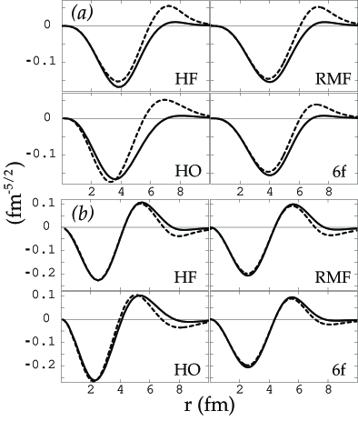
Figure 1: Numerical check of identities (11), (10). Comparison between $D_{\tilde{n}\tilde{\ell}j=\tilde{\ell}-{1\over 2}}g_{\tilde{n}\tilde{\ell}j=\tilde{\ell}-{1\over 2}}$ (dashed line) and $D_{\tilde{n}\tilde{\ell}j=\tilde{\ell}+{1\over 2}}g_{\tilde{n}\tilde{\ell}j=\tilde{\ell}+{1\over 2}}$ (solid line) for $1\tilde{f}$ (a) and $2\tilde{d}$ (b) pseudospin doublets in ²⁰⁸Pb obtained in different methods: HF, HO and RMF. The plot labeled ‘6f’ shows 6 times scaled lower components of the RMF wave function, see Eq. (15) and related discussion.

For the spherical harmonic oscillator potential (or spherical Nilsson potential) we take the analitycal form of wave functions with an oscillator frequency $\hbar\omega=41/A^{1/3}$ [Mos57] . Then, one can express $D_{{\tilde{n}}{\tilde{\ell}}j}(r)g_{{\tilde{n}}{\tilde{\ell}}j}(r)$ defined by Eq. (11) as:

$$\begin{array}[]{lll}&&D_{{\tilde{n}}{\tilde{\ell}}j={\tilde{\ell}}-{1\over 2}}(r)g_{{\tilde{n}}{\tilde{\ell}}j={\tilde{\ell}}-{1\over 2}}(r)=\\ &&=~{}\displaystyle{\chi_{{\tilde{n}}{\tilde{\ell}}}(x)\ \sum_{a=0}^{{\tilde{n}}-1}\frac{(-1)^{a}(2{\tilde{n}}+{\tilde{\ell}}-3/2-a)x^{a}}{({\tilde{n}}-1-a)!a!\Gamma(a+{\tilde{\ell}}+3/2)}},\\ \\ &&D_{{\tilde{n}}{\tilde{\ell}}j={\tilde{\ell}}+{1\over 2}}(r)g_{{\tilde{n}}{\tilde{\ell}}j={\tilde{\ell}}+{1\over 2}}(r)=\sqrt{\frac{{\tilde{n}}+{\tilde{\ell}}-1/2}{{\tilde{n}}-1}}\times\\ &&\times~{}\displaystyle{\chi_{{\tilde{n}}{\tilde{\ell}}}(x)\ \sum_{a=0}^{{\tilde{n}}-1}\frac{(-1)^{a}(2{\tilde{n}}-2-a)x^{a}}{({\tilde{n}}-1-a)!a!\Gamma(a+{\tilde{\ell}}+3/2)}},\end{array}$$ (16)

where the envelope function is

$$\chi_{{\tilde{n}}{\tilde{\ell}}}(x)=\sqrt{\frac{2(2\nu)^{\frac{6-{\tilde{\ell}}}{2}}(n-1)!}{\Gamma({\tilde{n}}+{\tilde{\ell}}-1/2)^{3}}}x^{\frac{{\tilde{\ell}}}{2}}e^{-x/2},$$ (17)

and

$$x=r^{2}2\nu,~{}~{}~{}\nu=\frac{m\omega}{2\hbar^{2}}.$$ (18)

Expressions (16) can be presented as products

$$D_{{\tilde{n}}{\tilde{\ell}}j}(r)g_{{\tilde{n}},{\tilde{\ell}},j}(r)=\chi_{{\tilde{n}}{\tilde{\ell}}}(x)P_{{\tilde{n}}{\tilde{\ell}}j}(x)$$ (19)

of the common envelope function $\chi_{{\tilde{n}}{\tilde{\ell}}}(r)$ and a polynomials $P_{{\tilde{n}}{\tilde{\ell}}j}(x)$ with power expansion coefficients $A_{a}({\tilde{n}},{\tilde{\ell}},j)$:

$$P_{{\tilde{n}}{\tilde{\ell}}j}(x)=\sum_{a=0}^{\tilde{n}-1}(-1)^{a}A_{a}({\tilde{n}},{\tilde{\ell}},j)\ x^{a}.$$ (20)

As seen from Eq. (20) these polynomials are of the same order $({\tilde{n}}-1)$ independent of $j$, whereas the original harmonic oscillator eigenfunction with $j={\tilde{\ell}}-{1\over 2}$ involves a polynomial of order ${\tilde{n}}$ while the harmonic oscillator eigenfunction with $j={\tilde{\ell}}+{1\over 2}$ involves a polynomial of order ${\tilde{n}}-1$ in $x$.

As an example, in the lower left corners of Fig. 1 (a) and (b) we compare $D_{{\tilde{n}}{\tilde{\ell}}j={\tilde{\ell}}+{1\over 2}}(r)g_{{\tilde{n}}{\tilde{\ell}}j={\tilde{\ell}}+{1\over 2}}(r)$ (dashed line) with $D_{{\tilde{n}}{\tilde{\ell}}j={\tilde{\ell}}-{1\over 2}}(r)g_{{\tilde{n}}{\tilde{\ell}}j={\tilde{\ell}}-{1\over 2}}(r)$ (solid line) using expression (16) or its equivalent (19). It is seen that $D_{{\tilde{n}}{\tilde{\ell}}j={\tilde{\ell}}+{1\over 2}}(r)g_{{\tilde{n}}{\tilde{\ell}}j={\tilde{\ell}}+{1\over 2}}(r)\approx D_{{\tilde{n}}{\tilde{\ell}}j={\tilde{\ell}}-{1\over 2}}(r)g_{{\tilde{n}}{\tilde{\ell}}j={\tilde{\ell}}-{1\over 2}}(r)$ in the whole range of $r$ considered.

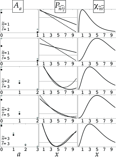
Figure 2: Structure of $D_{\tilde{n}\tilde{\ell}j}g_{\tilde{n}\tilde{\ell}j}$ for $j$=$\ell$–${1\over 2}$ (dashed line, grey points), $j$=$\ell$+${1\over 2}$ (solid line, black points) obtained in the harmonic oscillator model for different pairs $\tilde{n},\tilde{\ell}$ in ²⁰⁸Pb. The first column shows absolute values of coefficients $A_{a}$ (Eqs. (19, 20)) as a function of $a$. The second column shows $P_{\tilde{n}\tilde{\ell}}$, third column - envelope functions $\chi_{\tilde{n}\tilde{\ell}}$; both in terms of dimensionless variable $x$, defined in equation (18).

Systematic calculations of many states and nuclei have shown that relation (11) holds better as ${\tilde{n}}$ increases or ${\tilde{\ell}}$ decreases. In order to understand this property we can use the analytical results from Eq. (19). For this purpose plots of $P_{{\tilde{n}}{\tilde{\ell}}j}(x),~{}A_{a}({\tilde{n}},{\tilde{\ell}},j)$ are presented in Fig. 2. It is seen that $P_{{\tilde{n}}{\tilde{\ell}}j={\tilde{\ell}}-{1\over 2}}(x)$ and $P_{{\tilde{n}}{\tilde{\ell}}j={\tilde{\ell}}+{1\over 2}}(x)$ are overlapping more with ${\tilde{n}}$ increasing. While the quantum number ${\tilde{n}}$ is responsible for the similarities between polynomials, the envelope functions $\chi_{{\tilde{n}}{\tilde{\ell}}}(r)$ strongly depend on ${\tilde{\ell}}$. The higher ${\tilde{\ell}}$ is the broader is the ‘bell’ of $\chi_{{\tilde{n}}{\tilde{\ell}}}(r)$. Consequently, when ${\tilde{\ell}}$ decreases, the differences between $D_{{\tilde{n}}{\tilde{\ell}}j={\tilde{\ell}}+{1\over 2}}(r)g_{{\tilde{n}}{\tilde{\ell}}j={\tilde{\ell}}+{1\over 2}}(r)$ and $D_{{\tilde{n}}{\tilde{\ell}}j={\tilde{\ell}}-{1\over 2}}(r)g_{{\tilde{n}}{\tilde{\ell}}j={\tilde{\ell}}-{1\over 2}}(r)$ are reduced in the region where $P_{{\tilde{n}}{\tilde{\ell}}j={\tilde{\ell}}+{1\over 2}}(x)$ and $P_{{\tilde{n}}{\tilde{\ell}}j={\tilde{\ell}}-{1\over 2}}(x)$ differ. In general, when ${\tilde{n}}\gg{\tilde{\ell}}$, then $A_{a}({\tilde{n}},{\tilde{\ell}},j={\tilde{\ell}}-{1\over 2})\approx A_{a}({\tilde{n}},{\tilde{\ell}},j={\tilde{\ell}}+{1\over 2})$ and hence $D_{{\tilde{n}}{\tilde{\ell}}j={\tilde{\ell}}-{1\over 2}}(r)g_{{\tilde{n}}{\tilde{\ell}}j={\tilde{\ell}}-{1\over 2}}(r)\approx D_{{\tilde{n}}{\tilde{\ell}}j={\tilde{\ell}}+{1\over 2}}(r)g_{{\tilde{n}}{\tilde{\ell}}j={\tilde{\ell}}+{1\over 2}}(r)$.

III.2 Comparison within self–consistent models

In Figs. 1 (a) and (b) we plot $D_{{\tilde{n}}{\tilde{\ell}}j={\tilde{\ell}}+{1\over 2}}(r)g_{{\tilde{n}}{\tilde{\ell}}j={\tilde{\ell}}+{1\over 2}}(r)$ (dashed line) and $D_{{\tilde{n}}{\tilde{\ell}}j={\tilde{\ell}}-{1\over 2}}(r)g_{{\tilde{n}}{\tilde{\ell}}j={\tilde{\ell}}-{1\over 2}}(r)$ (solid line) using the HO model, the non-relativistic HF approximation, and the RMF approximation.

Comparing the non-relativistic and relativistic mean field results we see that the agreement is comparable or slightly better than the harmonic oscillator results. Therefore, the pseudospin symmetry relations are not only approximately valid for the relativistic mean field eigenfunctions but also for the non-relativistic HF eigenfunctions. Hence we seem to have pseudospin dynamic symmetry, that is, the energy levels are not degenerate but the eigenfunctions preserve the pseudospin symmetry.

In order to confirm that the radial wave functions of the lower components are approximately equal within a doublet we also plot them in the case of RMF calculations in the lower right corner of Figs. 1 (a) and (b). We multiply these wave functions by a factor of 6 in order to be comparable to the upper components as suggested by Eq. (15). Indeed the amplitudes of the lower components are approximately equal [Gin98] .

IV Spin symmetry and the Dirac Hamiltonian

IV.1 Spin Conditions on the Dirac Eigenfunctions

The Dirac Hamiltonian is invariant under an SU(2) algebra if the scalar potential, $V_{S}({\bf r})$, and the vector potential $V_{V}(\vec{r_{i}})$, are related [Bel75] ; [Gin97] ; [Pag01] :

$$V_{S}({\bf r})-V_{V}({\bf r})=C_{s},$$ (21)

where $C_{s}$ is a constant. Hence spin symmetry can occur for very relativistic systems like quarks in a meson where both $V_{S}({\bf r})$ and $V_{V}({\bf r})$ are large [Pag01] .

The spin generators

$${\bf{S}}=\left(\begin{array}[]{cc}{\bf{s}}&0\\ 0&{\bf{\tilde{s}}}\end{array}\right)$$ (22)

form an SU(2) algebra

$$[{S}_{i},{S}_{j}]=i\epsilon_{ijk}\ {S}_{k},$$ (23)

and commute with the Dirac Hamiltonian $H_{s}$ satisfying conditions (21)

$$[{S}_{i},H_{s}]=0.$$ (24)

Thus the operators ${S}_{i}$ generate an SU(2) invariant symmetry of $H_{s}$. Therefore, each eigenstate of the Dirac Hamiltonian $H_{s}$ has a partner with the same energy,

$$H_{s}\ \Phi_{k{\mu}}^{s}({\bf r})=E_{k}\Phi_{k{\mu}}^{s}({\bf r}),$$ (25)

where $k$ are the other quantum numbers and ${\mu}=\pm{1\over 2}$ is the eigenvalue of ${S}_{z}$,

$${S}_{z}\ \Phi_{k{\mu}}^{s}({\bf r})={\mu}\ \Phi_{k{\mu}}^{s}({\bf r}).$$ (26)

The eigenstates in the spin doublet will be connected by the generators ${S}_{\pm}$,

$${S}_{\pm}\ \Phi_{k{\mu}}^{s}({\bf r})=\sqrt{{\left({1\over 2}\mp{\mu}\right)({3\over 2}\pm{\mu})}}\ \Phi_{k{\mu}\pm 1}^{s}({\bf r}).$$ (27)

The generators (26), (27) do not mix upper and lower components. Since the spin operates on the upper components only, one of predictions of this symmetry is that the radial wave functions of the upper components of the Dirac eigenfunctions are identical. In the spherical symmetry limit the Dirac eigenfunctions then have the form

$$\Phi^{s}_{{n}_{r},{\ell},j,m}({\vec{r}})=\ \left(\begin{array}[]{c}g_{n\ell}(r)\ [Y^{({\ell})}(\theta,\phi)\ \chi]^{(j)}_{m}\\ if_{n\ell j}(r)\ [Y^{({\ell}_{j})}(\theta,\phi)\ \chi]^{(j)}_{m}\end{array}\right),$$ (28)

where ${\ell}_{j}={\ell}\pm 1$ for $j={\ell}\pm{1\over 2}$.

The spin generators (22) are related to the pseudospin generators by $\bf{S}=\gamma_{5}\bf{\tilde{S}}\gamma_{5}$ where $\gamma_{5}=\left(\begin{array}[]{cc}{0}&1\\ 1&0\end{array}\right).$ Therefore, the conditions are the same as for the pseudospin except that now ${\tilde{n}}\rightarrow n,{\tilde{\ell}}\rightarrow\ell,g(r)\rightarrow f(r),f(r)\rightarrow g(r)$:

$$D_{{n}{\ell}j={\ell}-{1\over 2}}(r)\ f_{{n}{\ell}j={\ell}-{1\over 2}}(r)={}$$ (29)

$${}=D_{n\ell j={\ell}+{1\over 2}}(r)f_{{n}{\ell}j={\ell}+{1\over 2}}(r)$$

and

$$g_{{n}{\ell}j={\ell}-{1\over 2}}(r)=g_{{n}{\ell}j={\ell}+{1\over 2}}(r).$$ (30)

For finite nuclei $C_{s}=0$ in Eq. (21) because the potentials go to zero for large $r$. Consequently, equality $V_{S}(r)=V_{V}(r)$ emerges in the spin symmetry limit. Therefore, we do not expect spin symmetry to be conserved in nuclei since it is known that $V_{S}(r)$ and $V_{V}(r)$ are both large and of opposite sign.

IV.2 Spin breaking for different models

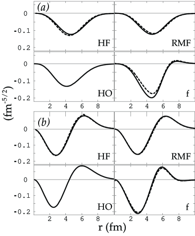
Figure 3: $1f$ (a) and $2d$ (b) spin partners’ wave functions of ²⁰⁸Pb obtained in HF, HO, and RMF calculations. The plot labeled ‘f’ shows the scaled values of $D_{n\ell j=\ell-{1\over 2}}g_{n\ell j=\ell-{1\over 2}}$ (dashed line) and $D_{n\ell j=\ell+{1\over 2}}g_{n\ell j=\ell+{1\over 2}}$ (solid line). See text for details.

In Figs. 3 (a) and (b) we plot the upper components $g_{n\ell j=\ell+{1\over 2}}(r)$ (dashed line) and $g_{n\ell j=\ell-{1\over 2}}(r)$ (solid line) using the HO model, the non-relativistic HF approximation, and the RMF approximation. The Nilsson model (HO) shows perfect agreement of course since it has a constant spin-orbit potential. However even the self-consistent non-relativistic and relativistic mean fields show very little difference between eigenstates of the spin doublets.

In the lower right-hand part of Figs. 3 (a) and (b), we compare $\lambda_{n\ell j={\ell}-{1\over 2}}D_{{n}{\ell}j={\ell}-{1\over 2}}(r)\ f_{{n}{\ell}j={\ell}-{1\over 2}}(r)$ with $\lambda_{n\ell j={\ell}+{1\over 2}}D_{n\ell j={\ell}+{1\over 2}}(r)f_{{n}{\ell}j={\ell}+{1\over 2}}(r)$ where the factor of $\lambda_{n\ell j}=({V_{S}(0)+V_{V}(0)+E_{n\ell j}})^{-1}$ scales the expression to be comparable in magnitude to the upper components, according to equation (14). The agreement for these differential relations is also very good.

V Summary and Conclusions

In the pseudospin symmetry limit the radial wave functions of the upper components of pseudospin doublets satisfy certain differential relations. We demonstrated that these relations are not only approximately valid for the relativistic mean field eigenfunctions but also for the non-relativistic Hartree-Fock and harmonic oscillator eigenfunctions. Generally, we expect them to be approximately valid for eigenfunctions of any non-relativistic phenomenological nuclear potential that fits the spin-orbit splittings of nuclei. Likewise in the spin symmetry limit the radial amplitudes of the upper components of the Dirac eigenfunctions of spin doublets are predicted to be equal and this is approximately valid for both non-relativistic and relativistic mean field models. Also the spatial amplitudes of the lower components of the Dirac eigenfunctions of spin doublets satisfy differential relations in spin symmetry limit and these relations are approximately valid in the relativistic mean field model.

Hence we seem to have both spin and pseudospin dynamic symmetry; that is, the energy levels are not degenerate but the eigenfunctions well preserve both symmetries. For both of these symmetries to be conserved both the vector and scalar potentials must be constant. Of course this is not true. However, for heavy nuclei this is approximately true in the nuclear interior and exterior. Only on the surface are the potentials changing rapidly. This leads to a dynamic symmetry for both spin and pseudospin. The spin-orbit splittings are determined by $d[V_{V}(r)-V_{S}(r)]/dr$ while the pseudospin-orbit splittings are determined by $d[V_{V}(r)+V_{S}(r)]/dr$. Therefore, the energy splittings for spin doublets are larger than for pseudospin doublets because $V_{V}(r)-V_{S}(r)$ changes more rapidly on the nuclear surface than $V_{S}(r)+V_{V}(r)$ because $V_{V}(r)-V_{S}(r)\gg|V_{S}(r)+V_{V}(r)|$ in the interior and both go to zero in the nuclear exterior.

References

(1)
K.T. Hecht and A. Adler, Nucl. Phys. A137, 129 (1969).
(2)
A. Arima, M. Harvey, and K. Shimizu, Phys. Lett. 30B, 517 (1969).
(3)
W.P. Jones, L.W. Borgman, K.T. Hecht, J. Bardwick, and W.C. Parkinson,
Phys. Rev. C4 580 (1971).
(4)
F.T. Baker and R. Tickle, Phys. Rev. C5 182 (1972).
(7)
A. Bohr, I. Hamamoto, and B.R. Mottelson, Phys. Scr. 26, 267 (1982).
(8)
J. Dudek, W. Nazarewicz, Z. Szymański, and G.A. Leander,
Phys. Rev. Lett. 59, 1405 (1987).
(9)
D. Troltenier, W. Nazarewicz, Z. Szymański, and J.P. Draayer,
Nucl. Phys. A567, 591 (1994).
(10)
A.E. Stuchbery, J. Phys. G25, 611 (1999).
(11)
A.E. Stuchbery, Nucl. Phys. A700, 83 (2002).
(12)
W. Nazarewicz, P.J. Twin, P. Fallon, and J.D. Garrett, Phys. Rev. Lett. 64, 1654 (1990).
(13)
F.S. Stephens, M.A. Deleplanque, J.E. Draper, R.M. Diamond, A.O. Macchiavelli,
C.W. Beausang, W. Korten, W.H. Kelly, F. Azaiez, J.A. Becker, E.A. Henry,
S.W. Yates, M.J. Brinkman, A. Kuhnert, and J.A. Cizewski,
Phys. Rev. Lett. 65, 301 (1990).
(14)
A.L. Blokhin, C. Bahri, and J.P. Draayer, Phys. Rev. Lett. 74, 4149
(1995).
(15)
J.N. Ginocchio, Phys. Rev. Lett. 78, 436 (1997).
(16)
T.D. Cohen, R.J. Furnstahl, and D.K. Griegel, Phys. Rev. Let. 67, 961
(1991).
(17)
J.N. Ginocchio and A. Leviatan, Phys. Lett. B 425, 1 (1998).