[1]∂_#1 [2]— #1 ⟩ ⟨#2 — [4]— #1 ⟩ ⟨#2 — #3 ⟩ ⟨#4 — [2]⟨#1 — #2 ⟩ [3]⟨#1 — #2 — #3 ⟩ [2][ #1 ,   #2 ] [2]{ #1 ,   #2 } [1]X_#1 [1]Y_#1 [1]Z_#1

Introduction

Over the past century, the laws of equilibrium statistical mechanics have been increasingly understood and organized via a Wilsonian renormalization group [1, 2]. However, beyond the familiar setting of equilibrium, new phenomena can arise—e.g., spontaneous symmetry breaking in models of flocks birds in two spatial dimensions, which is not possible in equilibrium due to the Mermin-Wagner theorem. Such classical systems fall under the umbrella of active matter [3, 4, 5]— i.e., systems whose constituent particles are “self propelled” (i.e., contain internal sources of energy and entropy)—which has led to a significant body of research into nonequilibrium classical phenomena.

Quantum systems may also be driven away from thermal equilibrium. Indeed, one may directly try to add quantum fluctuations to a theory of classical active matter, such as flocking [6, 7, 8]. However, this is certainly not the only setting in which nonequilibrium quantum systems may arise. For example, it is well established [9] that systems may tend towards entangled states in a driven-dissipative system, described in terms of open quantum dynamics where a coherently driven system is coupled to an environment or bath. But perhaps the most important example of a uniquely quantum system driven out of thermal equilibrium would be a future quantum computer. If such a quantum computer is built out of, for example, surface code qubits [10, 11], such a system will not store quantum information if it thermalizes – an analogue of a “Mermin-Wagner theorem” forbids this in two spatial dimensions [12]. Therefore, the storage of quantum information over long times (in a surface code) requires “activity,” namely being persistently driven out of equilibrium.

The purpose of this paper is to give a systematic framework for discovering and, just as importantly, organizing our understanding of these “active” quantum systems. Inspired by recent work [13] in classical statistical physics, which provides a framework for classifying systems based on their steady-state probability distribution, here we provide an exhaustive classification of the most general local quantum many-body system that protects a target stationary (mixed) state $\sigma$. When $\log\sigma$ is a sum of commuting operators (i.e., $\sigma$ is a “stabilizer state”), we can find (almost all) local many-body dynamics that protects the desired state. An immediate, and sometimes useful, byproduct of this framework is a definition of time-reversal symmetry for such open quantum systems; this definition has independently been identified in [14].

Solving this technical problem is rather useful, as it immediately provides us with new (and unifying!) insight into a diverse array of problems from different subfields within physics.

In condensed matter and quantum statistical mechanics, there has been intense recent interest in discovering uniquely quantum nonequilibrium phases in monitored quantum systems, in which unitary dynamics is interrupted by measurements [15, 16, 17, 18, 19, 20]. In order to avoid a postselection problem and realize novel phases in the thermodynamic limit of any experiment, it is crucial to perform quantum error correction (i.e., active feedback) based on the measurement outcomes to drive the system towards a deterministic state whose properties can be measured in experiment [21, 22, 23, 24, 25, 26, 27, 28]. However, it is not a priori obvious whether such a phase realizes a uniquely quantum state of matter, or whether it is essentially a classical phase that arises out of a microscopically quantum dynamical system. Although we do not attempt to definitively answer such a large open question in this paper, we believe that the framework we provide in this work is a well-defined starting point for addressing such questions systematically.

In quantum information sciences, it is often desirable to protect entangled states against decoherence or other deleterious environmental effects. For example, we may wish to prepare an entangled GHZ state [29], which is capable of performing quantum-enhanced sensing [30]. Alternatively, as highlighted previously, we may want to protect a quantum error-correcting code [31, 32]. Usually, one devises some protocol that relies on few-qubit measurements and operations in order to protect such a code state, and then numerically simulates whether or not the protocol can protect against errors. The formalism that we describe here is very well-suited for discovering fault-tolerant quantum error correcting protocols, and gives a systematic way of building all possible driven-dissipative systems that protect a target state $\sigma$.

Lastly, one anticipated application of future quantum computers is to simulate properties of quantum systems arising in physics, material science, and chemistry [33]. In many perceivable cases (such as correlation functions or transport properties), preparing ground states or thermal states has been identified as a key algorithmic subroutine. Nevertheless, the complexity of practically relevant low-energy states has remained a debated topic, and thus far, there has not been a consensus on the “go-to” state preparation algorithm [34] (see e.g., [35, Table 1] for a catalog). Recently, there is a new algorithmic family of quantum Gibbs samplers [36, 37, 38, 35, 39] that attempts to model and simulate the thermalization process in Nature. The challenge is that, in noncommuting Hamiltonian, the energy uncertainty, locality, and quantum detailed balance appear to be in tension; the conventional Davies’ generator is inefficient in noncommuting many-body systems, and only recently has this been reconciled [39, 40, 41]. Although we have mostly focused on commuting Hamiltonians, the formalism described in this paper should, in principle, give an “exhaustive” classification of all possible ways to find noncommutative Gibbs samplers. Since in classical statistical physics, the convergence rate of such samplers is often increased by breaking time-reversal symmetry [42, 43], it is natural to expect that a similar result also holds in quantum systems. Our framework explains how to look for these T-broken samplers that still protect the same state.

Reversibility and effective theories of open systems

We now review some preliminary facts about dissipative (open) systems in both the classical and quantum settings. As previously emphasized, in both cases, we organize our approach around the identification of a target stationary state, as in the related work [13] for classical systems. This section serves to explain some of our physical motivations underlying this work, though readers primarily interested in the problem of engineering open systems with known steady states may skip to the formalism in Sec. 3.

Because we assume that the open dynamics of interest are time-translation invariant, such a stationary state always exists. The existence of this stationary state implies a reversibility transformation, which we associate with microscopic time reversal. Precise definitions of reversibility can be found in later subsections. One commonly defines a system to be in equilibrium if the dynamics is reversible; since our framework is organized around a known steady state, it is straightforward to distinguish equilibrium versus nonequilibrium phenomena. Generalizing this reversibility symmetry to include additional transformations (e.g., spatial inversion) is straightforward. Given a target stationary state and any symmetries (especially reversibility) that we wish to impose, we can work out the most general possible local unitary and dissipative dynamics compatible therewith. This approach embodies the spirit of Wilson’s effective (field) theory [1, 2, 13], and is central to our framework.

Classical systems

We begin by reviewing the Wilsonian approach [1, 2] for classical systems in the presence of dissipation that relax to a known (or target) stationary state $\sigma$ [13]. For simplicity, we focus on classical systems with discrete state spaces (e.g., a collection of $N$ Ising spins). The dynamics correspond to a continuous-time Markov process captured by a master equation [44, 45, 46, 47, 48] – i.e., a discrete analogue of the Fokker-Planck equation [48, 49, 50, 51]. Denoting by $W_{ba}$ the rate at which state $a$ transitions to state $b\neq a$, we have that

$$W_{aa}=-\sum_{b,b\neq a}W_{ba}\,,~{}~{}$$ (1)

is the rate at which the system remains in state $a$. The system evolves via the classical master equation,

$$\partial^{\vphantom{\dagger}}_{t}p_{a}(t)=\sum\limits_{b}W_{ab}p_{b}(t)\,,~{}~{}$$ (2)

where $p_{a}(t)$ is the probability to find the system in configuration $a$ at time $t$. The stationary state $\sigma$ is a probability distribution (with probability $\sigma_{a}$ for configuration $a$) such that

$$\partial^{\vphantom{\dagger}}_{t}\sigma=W\sigma=0\,,~{}~{}$$ (3)

where above, $W$ is the rate matrix and $\sigma$ is a vector whose components are the probabilities $\sigma_{a}$. We also define the probability to go from the initial state $a$ to the final state $b$ in time $t$ under $W$ as

$$\text{Pr}\left[a(0)\to b(t);W\right]=\left\langle*\middle|b\middle|\mathrm{e}^{tW}\right\rangle{a}\,,~{}~{}$$ (4)

since $W$ is time independent; this quantity is also known as the “propagator” [13].

Importantly, the existence of a stationary distribution $\sigma$ (3) – which need not correspond to thermal equilibrium – implies the global balance condition [52, 53, 13]

$$\sum_{b,b\neq a}\left[\sigma_{b}W_{ab}-W_{ba}\sigma_{a}\right]=0\,,~{}~{}$$ (5)

for any configuration $a$, so that the total probability to transition into configuration $a$ in the stationary state $\sigma$ is equal to the total probability to transition out of configuration $a$. From the global balance condition (5), we identify the time-reversed transition matrix

$$\widetilde{W}_{ba}=\sigma_{b}W_{ab}/\sigma_{a}~{}~{}~{}\Longleftrightarrow~{}~{}~{}\widetilde{W}=\hat{\sigma}^{-1}\,W^{T}\,\hat{\sigma}\,,~{}~{}$$ (6)

where $\hat{\sigma}_{ab}=\sigma_{a}\delta_{ab}$ is the “stationary operator,” $W$ and $\widetilde{W}$ share the same stationary distribution $\sigma$ (3), and crucially, if the former generates the sequence of states $a,b,\ldots,y,z$ then the latter realizes the reversed sequence of states $z,y,\ldots,b,a$. Moreover, noting that $\left\langle*\middle|b\middle|W\right\rangle{a}=\left\langle*\middle|a\middle|W^{T}\right\rangle{b}$, we have that

$$\text{Pr}\left[a(0)\to b(t);W\right]=\left\langle*\middle|a\middle|\mathrm{e}^{tW^{T}}\right\rangle{b}=\left\langle*\middle|a\middle|\hat{\sigma}^{-1}\mathrm{e}^{t\widetilde{W}}\hat{\sigma}\right\rangle{b}=\mathrm{e}^{\Phi(a)-\Phi(b)}\,\text{Pr}\left[b(0)\to a(t);\widetilde{W}\right]\,,~{}~{}$$ (7)

since the operator $\hat{\sigma}$ acts as $\mathrm{e}^{\Phi(b)}$ on the configuration $b$, so that the probability to go from $a\to b$ in time $t$ under $W$ is related to the probability to go from $b\to a$ in time $t$ under the time-reversed generator $\widetilde{W}$, up to the ratio of the probabilities for those configurations in the stationary distribution $\sigma$ [13].

Accordingly, we associate the $\mathbb{Z}_{2}$ “reversibility” transformation,

$$\text{T}:W\mapsto\widetilde{W}\,,~{}~{}$$ (8)

with time reversal [13]. For discrete state spaces, T (8) corresponds exactly to time reversal, as it maps the Markov generator $W$ to its time-reversed partner $\widetilde{W}$. However, for continuous state spaces described by the Fokker-Planck equation, we also combine T (8) with “microscopic” $\mathbb{Z}_{2}$ transformations on certain variables (e.g., the momentum transforms as $p\to-p$). Below, T is assumed to include any additional required transformations. As a reminder, the existence of the stationary state $\sigma$ implies the transformation T (8) and time-reversed generator $\widetilde{W}$ (6) [13, 52, 53].

We define a dynamical system as “equilibrium” dynamics when it is even under T – i.e., $W=\widetilde{W}$. One often states that (6) implies that T-even systems obey detailed balance:

$$\sigma_{b}W_{ab}=\sigma_{a}W_{ba}~{}~{}$$ (9)

if and only if $W=\widetilde{W}$. We emphasize, however, that detailed balance is not necessary for global balance. There are many stochastic dynamical systems that break time-reversal symmetry T – i.e., for which $W\neq\widetilde{W}$, while maintaining the same stationary state $\sigma$. In many physical cases of interest, one can identify an extra $\mathbb{Z}_{2}$ transformation g (e.g., parity, charge conjugation, etc.) such that the product of g and T is a symmetry of the dynamics. We refer to this combined $\mathbb{Z}_{2}$ symmetry gT as generalized time reversal, and in the classical setting, it is quite instructive to classify dynamics according to whether they respect, explicitly (or spontaneously) break T and/or gT [13]. Finally, we comment that it is possible to enforce generic (e.g., continuous) symmetries – in both a weak and strong sense – on the generator W [13].

Quantum systems

We now consider the quantum analogues to the discussion of open classical systems in Sec. 2.1. As before, we require continuous time-translation symmetry. We also take the bath to be Markovian (i.e., memoryless), as is standard in the literature on open quantum systems [54, 55, 56, 57, 58, 59, 60, 61]. Although we only explicitly consider finite-dimensional quantum systems throughout, we see no conceptual barrier to extending the framework to infinite-dimensional quantum systems, such as bosonic modes. A somewhat similar philosophy was discussed in the context of noninteracting systems in [62].

The quantum analogue of the probability distribution $p(t)$ is the reduced density matrix $\rho(t)$, which captures the (generically mixed) state of the quantum system at time $t$ (e.g., after tracing over environmental degrees of freedom). The set of allowed updates to a density matrix $\rho$ correspond to completely positive and trace-preserving (CPTP) maps [63]. The quantum analogue of the master equation (2) for classical systems is the Lindblad master equation [54, 55, 56, 57, 58, 59, 60, 61], which captures generic CPTP maps. Such dynamics are generated by a “Lindbladian” (or “Liouvillian”) $\mathcal{L}$ of the general form

$$\partial^{\vphantom{\dagger}}_{t}\rho=\mathcal{L}(\rho)=-\mathrm{i}[H,\rho]+\sum\limits_{i,j}\gamma_{ij}\left(A^{\vphantom{\dagger}}_{i}\rho A_{j}^{\dagger}-\frac{1}{2}\ \{A_{j}^{\dagger}A^{\vphantom{\dagger}}_{i},\rho\}\right)\,,$$ (10)

where $\gamma_{ij}$ is a positive-semidefinite matrix, the “jump operators” $\{A_{i}\}$ form a complete basis for the operators acting on the system’s Hilbert space, and the system Hamiltonian $H$ is Hermitian, and may differ from the naïve Hamiltonian $H_{0}$ for the system in isolation (i.e., integrating over the bath degrees of freedom to recover $H$ may “renormalize” terms in $H_{0}$ or generate new ones).

We also comment that the choice of $H$ and the dissipative part $\gamma$ is not unique. However, if we require that $H$ and the jump operators $\{A_{i}\}$ are all traceless, then the Lindbladian (10) is unique, up to a change of basis on the jump operators $A_{i}$. Due to time-translation symmetry of $\mathcal{L}$ (10), an initial density matrix $\rho$ at time $t=0$ evolves under to the state $\rho(t)=\mathrm{e}^{t\mathcal{L}}\rho$ at time $t$.

As in the classical setting, we seek Lindbladians $\mathcal{L}$ that protect a target stationary density matrix $\sigma$, which we assume is mixed. The stationarity condition (3) for the quantum case corresponds to

$$\mathcal{L}(\sigma)=0\,,~{}~{}$$ (11)

where we find it convenient to write the stationary state $\sigma$ in the particular form

$$\sigma=\mathrm{e}^{-\Phi}\,,~{}~{}$$ (12)

where we stress the following points about the stationary state $\sigma$ and the corresponding $\Phi$:

1. We assume that $\sigma$ (12) is full rank – and thus, invertible. However, our results also extend to pure states upon writing $\Phi=\beta H_{\text{eff}}$ and taking the limit $\beta\to\infty$.

2. We only require that $\sigma>0$ is positive definite, which is guaranteed when $\Phi=\Phi^{\dagger}$ is Hermitian and bounded.

3. For convenience of presentation and without loss of generality, we neglect the overall normalization of $\sigma$ (12), which is unimportant to the linear functions of $\sigma$ that we consider herein.

4. Most importantly, the operator $\Phi$ is generically unrelated to the Hamiltonian $H$ that generates the unitary part of the time evolution captured by $\mathcal{L}$ (10).

In Sec. 3.2, we build generic Lindbladians $\mathcal{L}$ that preserve a target stationary state $\sigma$ (12). This is a departure from the standard approach in the literature, in which one firsts postulate the form of $H$, $A_{i}$, and $\gamma_{ij}$ based on microscopic, phenomenological assumptions about locality, symmetries, and the dominant dynamical processes present in real experiments on a given system. As Ref. 13 argues in the context of classical systems, it is often more instructive to take the “inverse perspective”: rather than try to deduce $\sigma$ from $\mathcal{L}$ (10), we instead identify all Lindbladians $\mathcal{L}$ compatible with a particular choice of $\sigma$ (12).

As in the classical case, we also define a reversibility transformation (8) that we associate with a time-reversal transformation with respect to a stationary density matrix $\sigma$ of interest. Before making this transformation precise, we first define several inner products, along with the adjoint Lindbladian $\mathcal{L}^{\dagger}$.

First, consider the standard “Frobenius” operator inner product, defined by

$$\langle A,B\rangle\equiv\frac{1}{D}\operatorname{tr}(A^{\dagger}\hskip 1.13809ptB)\,,~{}~{}$$ (13)

where $D=\operatorname{tr}(\mathds{1})$ is the dimension of the underlying Hilbert space $\mathcal{H}$. When $D$ is finite, the space $\text{End}(\mathcal{H})$ of operators on $\mathcal{H}$ is itself a Hilbert space with dimension $D^{2}$, since all operators on $\mathbb{C}^{D}$ are bounded and trace class. When $\mathcal{H}$ corresponds to a system of $N$ qubits, the Pauli group – i.e., the set of all Kronecker products of Pauli operators over $N$ qubits – forms an orthonormal basis with respect to (13).

Importantly, the Frobenius inner product (13) defines the adjoint Lindbladian $\mathcal{L}^{\dagger}$ via

$$\langle A,\mathcal{L}B\rangle=\frac{1}{D}\operatorname{tr}[A^{\dagger}\mathcal{L}(B)]=\frac{1}{D}\operatorname{tr}[B\mathcal{L}^{\dagger}(A^{\dagger})]=\operatorname{tr}[B^{\dagger}\mathcal{L}^{\dagger}(A)]^{*}=\langle B,\mathcal{L}^{\dagger}A\rangle^{*}=\langle\mathcal{L}^{\dagger}A,B\rangle\,,~{}~{}$$ (14)

where $\langle A,B\rangle^{*}=\langle B,A\rangle$ by skew symmetry of (13) under complex conjugation.

Physically, we interpret $\mathcal{L}$ (10) as the generator of time evolution of density matrices $\rho$ in the Schrödinger picture, and the adjoint Lindbladian $\mathcal{L}^{\dagger}$ (14) as the generator of time evolution of operators in the Heisenberg picture. In particular, consider the time-dependent expectation value

$$\langle O(t)\rangle=\operatorname{tr}[O\hskip 1.13809pt\rho(t)]=\operatorname{tr}[O\hskip 1.13809pt\mathrm{e}^{t\mathcal{L}}(\rho)]\equiv\operatorname{tr}[\rho\hskip 1.13809pt\mathrm{e}^{t\mathcal{L}^{\dagger}}(O)]=\operatorname{tr}[\rho\hskip 1.13809ptO(t)]\,,~{}~{}$$ (15)

where $\rho(t)=\mathrm{e}^{t\mathcal{L}}\rho$ and $O(t)=\mathrm{e}^{t\mathcal{L}^{\dagger}}O$ in the Schrödinger and Heisenberg pictures, respectively. Just as the Lindbladian $\mathcal{L}$ (10) annihilates the stationary state $\sigma$ (11), the adjoint satisfies

$$\mathcal{L}^{\dagger}(\mathds{1})=0\,,~{}~{}$$ (16)

as a result of $\mathcal{L}$ (10) being trace preserving – i.e., $1=\operatorname{tr}[\rho(t)]=\operatorname{tr}[\rho\hskip 1.13809pt\mathrm{e}^{t\mathcal{L}^{\dagger}}(\mathds{1})]$ for all times $t\geq 0$.

Before considering the quantum analogue of the reversibility transformation (8), we define another operator inner product. Physically, this inner product captures time-dependent correlation functions, i.e.,

$$\langle A(t),B\rangle_{\sigma}\equiv\operatorname{tr}\left[A^{\dagger}(t)\hskip 1.13809pt\sigma^{1/2}B\sigma^{1/2}\right]=\operatorname{tr}\left[\mathrm{e}^{t\mathcal{L}^{\dagger}}(A^{\dagger})\hskip 1.13809pt\mathcal{T}(B)\right]\,,~{}~{}$$ (17)

where we have implicitly defined the superoperator $\mathcal{T}$ via

$$\mathcal{T}(\rho)=\sigma^{1/2}\rho\hskip 1.13809pt\sigma^{1/2}\quad\text{and}\quad\mathcal{T}^{-1}(\rho)=\sigma^{-1/2}\rho\hskip 1.13809pt\sigma^{-1/2}\,,$$ (18)

where we have explicitly written the inverse $\mathcal{T}^{-1}$ for convenience. Applying the definition of the adjoint Lindbladian $\mathcal{L}^{\dagger}$ (14) and other manipulations to the inner product (17) leads to

$$\langle A(t),B\rangle_{\sigma} \equiv\operatorname{tr}\left[\mathrm{e}^{t\mathcal{L}^{\dagger}}(A^{\dagger})\hskip 1.13809pt\mathcal{T}(B)\right]=\operatorname{tr}\left[A^{\dagger}\hskip 1.13809pt\mathrm{e}^{t\mathcal{L}}(\mathcal{T}(B))\right]$$

$$=\operatorname{tr}\left[A^{\dagger}\hskip 1.13809pt\mathcal{T}\big{(}\mathrm{e}^{t\mathcal{T}^{-1}\mathcal{L}\mathcal{T}}(B)\big{)}\right]$$

$$=\operatorname{tr}\left[\mathrm{e}^{t\mathcal{T}^{-1}\mathcal{L}\mathcal{T}}(B^{\dagger})\hskip 1.13809pt\mathcal{T}(A)\right]^{*}$$

$$\equiv\operatorname{tr}\left[\mathrm{e}^{t\widetilde{\mathcal{L}}^{\dagger}}(B^{\dagger})\hskip 1.13809pt\mathcal{T}(A)\right]^{*}=\langle A,\widetilde{B(t)}\rangle_{\sigma}\,,~{}~{}$$ (19)

where, in the first line, we used the definition of the adjoint (14) to move the time evolution from $A^{\dagger}$ to $B$; in the second line, we pulled the superoperator $\mathcal{T}$ through the exponential of $\mathcal{L}$ (10); in the third line, we used the facts that $\operatorname{tr}[A\hskip 1.13809pt\mathcal{T}(B)]=\operatorname{tr}[A\hskip 1.13809pt\sigma^{1/2}B\hskip 1.13809pt\sigma^{1/2}]=\operatorname{tr}[\mathcal{T}(A)\hskip 1.13809ptB]$ and $\operatorname{tr}[O^{\dagger}]=\operatorname{tr}[O]^{*}$; in the final line, we defined a “reversed” Lindbladian $\widetilde{\mathcal{L}}$ as the adjoint with respect to the inner product (17), i.e.,

$$\text{T}\hskip 1.13809pt:\hskip 1.13809pt\mathcal{L}\mapsto\widetilde{\mathcal{L}}\equiv\mathcal{T}\hskip 1.13809pt\mathcal{L}^{\dagger}\mathcal{T}^{-1}\quad\,,~{}~{}$$ (20)

so that $\widetilde{B(t)}\equiv\mathrm{e}^{t\widetilde{\mathcal{L}}^{\dagger}}(B)$ in (19), and $\widetilde{\mathcal{L}}$ is analogous to the time-reversed generator $\widetilde{W}$ in the classical case (8). It is straightforward to verify that the transformation T (20) is $\mathbb{Z}_{2}$, as one expects of a time-reversal operation; accordingly, we identify $\widetilde{\mathcal{L}}$ (20) as the time-reversed partner to $\mathcal{L}$ (10), where

$$\widetilde{\mathcal{L}}(\rho)=\sigma^{1/2}\mathcal{L}^{\dagger}(\sigma^{-1/2}\rho\hskip 1.13809pt\sigma^{-1/2})\hskip 1.13809pt\sigma^{1/2}\,,~{}~{}$$ (21)

and we note that $\widetilde{\mathcal{L}}(\sigma)=\sigma^{1/2}\mathcal{L}^{\dagger}(\mathds{1})\hskip 1.13809pt\sigma^{1/2}=0$ by the trace-preserving condition (16), so that the time-reversed Lindbladian $\widetilde{\mathcal{L}}$ (20) has the same stationary state $\sigma$ (12) as the original Lindbladian $\mathcal{L}$ (10).

We also comment that the particular definition of the correlation-function inner product (17) is required for the time-reversed Lindbladian $\widetilde{\mathcal{L}}$ to be a valid CPTP map [66, 67]. More generally, one could instead define a family of correlation-function inner products (17) given by

$$\langle A(t),B\rangle_{\sigma,s}\equiv\operatorname{tr}\left[A^{\dagger}(t)\sigma^{s}B\hskip 1.13809pt\sigma^{1-s}\right]\,,~{}~{}$$ (22)

where the choices $s=0$ and $s=1/2$ are the most common in the literature. Although one can, in principle, define a time-reversal transformation T (20) with respect to the $s$-dependent inner product (22), it is only for the symmetric choice $s=1/2$ that $\widetilde{\mathcal{L}}$ is a valid Lindbladian [68, 66, 67]. For other choices of $s\neq 1/2$, $\widetilde{\mathcal{L}}$ fails to be completely positive. We also note that the symmetric $s=1/2$ correlation function is common in the analysis of correlations, locality, and spectral properties in chaotic systems [69, 27, 70].

Importantly, the $\mathbb{Z}_{2}$ transformation T (20) defines the notion of quantum detailed balance [66, 67]. An open quantum system with a Lindbladian $\mathcal{L}$ (10) is said to obey quantum detailed balance (QDB) if

$$\mathcal{L}(\rho)-\widetilde{\mathcal{L}}(\rho)=-2\mathrm{i}[H_{\sigma},\rho]\,,~{}~{}$$ (23)

for any $\rho$, where $H_{\sigma}$ commutes with the stationary state $\sigma$ (12) [66, 67]. Intuitively, open systems that relax to thermal stationary states – where $\Phi=\beta H$ (12) – are expected to obey QDB (23); the time-reversal operation T (20) flips the sign of the Hamiltonian term in $\widetilde{\mathcal{L}}$ compared to $\mathcal{L}$ (10), leading to (23) with $H_{\sigma}=H$. However, this definition of detailed balance also extends to generic (i.e., possibly nonthermal) stationary states $\sigma$ upon replacing $H$ with any $H_{\sigma}$ satisfying $[H_{\sigma},\sigma]=0$ in (23). Systems that obey QDB are straightforwardly described by the formalism we present in Sec. 3. In particular, the Lindblad dynamics of systems that relax to thermal equilibrium – with $\sigma\propto\exp(-\beta H)$ – is generically captured by Davies’ generator [71, 72], which we discuss in Sec. 3.1.2. However, we stress that the framework detailed in Sec. 3 extends beyond thermal systems, and even to those that break QDB (23).

Separately, we say that a Lindbladian $\mathcal{L}$ is T even if and only if

$$\mathcal{L}=\widetilde{\mathcal{L}}\quad\Longleftrightarrow\quad\langle A(t),B\rangle_{\sigma}=\langle A,B(t)\rangle_{\sigma}\,,~{}~{}$$ (24)

which differs slightly from the definition of quantum detailed balance, except when $H_{\sigma}=0$. Instead, being T even (24) is related to the Kubo-Martin-Schwinger (KMS) invariance [73, 74, 75, 76] of generic thermal systems. In fact, recent works extending the successes of thermal effective field theories (EFTs) [1, 2] to hydrodynamic systems and even beyond equilibrium have been organized around KMS invariance [77, 78, 79, 80, 81, 82, 83, 13].

In the context of open classical systems [13], the classification of dynamical generators $W$ (2) – and even particular terms in the generator – is crucial to the diagnosis of the possible phases of matter associated with a stationary distribution $\Phi$. In the classical setting, all terms corresponding to Hamiltonian dynamics (i.e., leading to equations of motion characterized by Poisson brackets) and all terms due to dissipation (i.e., coming from stochastic noise sources) are guaranteed to be even under classical T (8). Hence, (closed) Hamiltonian systems, those that relax to thermal stationary states $\sigma\propto\exp(-\beta H)$, and dissipative relaxation to thermal states are all T even. In the classical setting, these dynamics also obey KMS invariance and detailed balance. However, nonreciprocal (and even active) dynamics require the presence of terms in $W$ (2) that are odd under T (8). Physically, these terms do not result from integrating out degrees of freedom that are in thermal equilibrium with the system itself. In the context of self-propelled particles (e.g., birds), these additional nonthermal degrees of freedom correspond to internal “batteries,” which act as local sources and sinks of energy and entropy, potentially leading to nonthermal dynamics and stationary states, and even violations [84] of the Mermin-Wagner theorem [85].

We expect a similar analysis of open quantum systems – described by a Lindbladian $\mathcal{L}$ (10) – to be similarly fruitful. As in the classical setting, there are numerous definitions of T (20), detailed balance (23), and KMS invariance (24), which we discuss further in Sec. 2.4. In fact, there are arguably even more definitions for quantum systems. We also note that there are more ways to break these notions of T (and also QDB and KMS) in quantum systems, as both the “Hamiltonian” term and the dissipative jump operators in the Lindbladian (10) can be T odd, in contrast to the classical case. Moreover, as we discuss in Sec. 5.2, one can break T in ways that have classical analogues, and also in ways that are unique to the quantum setting. We relegate a classification of the nonequilibrium phases of open quantum systems and their corresponding dynamics to future work, though we expect notions of T (20) to play a crucial role.

Incorporating symmetries

Before discussing generalizations of the time-reversal transformation T (20), we first briefly discuss the notions of weak versus strong symmetries in open systems and the action of symmetry transformations on the dynamical generator $\mathcal{L}$ (10). In the following discussion, we primarily highlight comparisons to the effective theories of open classical systems [13] and the general action of symmetries on the Linbladian $\mathcal{L}$ (10) in abstract terms. Although we expect that the existence – and possibly, spontaneous breaking – of one or more symmetries is important to constructing effective theories of open quantum systems, in the applications to quantum error correction that we consider herein, there is generally no symmetry restriction on the terms in $\mathcal{L}$ (10). Hence, we only briefly discuss the constraints imposed by symmetries on $\mathcal{L}$ (10) when discussing applications to quantum error correction in Sec. 4.5.

In the context of open systems – both classical and quantum – there are two distinct notions of symmetries: weak and strong [86, 87, 13]. In the classical setting discussed in Sec. 2.1, symmetries are defined with respect to the Fokker-Planck generator $W$ (2). A strong symmetry of $W$ is one that holds on every stochastic trajectory, captured by the condition $\mathrm{e}^{-F}W\hskip 1.13809pt\mathrm{e}^{F}=W$ for some conserved “charge” $F(\boldsymbol{q})$, which is a functions of the coordinates $\boldsymbol{q}=\{q_{a}\}$. Conservation of $F$ (in the strong sense) is guaranteed provided that the operator $W$ (2) is invariant under shifting the differential operator according to $\partial^{\vphantom{\dagger}}_{*}{a}\to\partial^{\vphantom{\dagger}}_{*}{a}+[\partial^{\vphantom{\dagger}}_{*}{a}F]$ [13]. Conversely, a weak symmetry of $W$ is one that only holds on average, meaning that $\partial^{\vphantom{\dagger}}_{t}\langle F(\boldsymbol{q})\rangle=0$. This is guaranteed provided that $W^{T}F=0$ [13].

In open quantum systems, we again have both weak and strong notions of symmetries, which we now define explicitly. In particular, consider a symmetry group $G$, whose elements $g\in G$ have some unitary representation $U(g)$ acting on the Hilbert space $\mathcal{H}$ of interest. For each element $g\in G$, we define the left (L) and right (R) action of $g$ on a density operator $\rho$ via the following pair of superoperators:

$$\mathcal{U}_{g,\text{L}}(\rho) =U(g)\rho,$$ (25a)

$$\mathcal{U}_{g,\text{R}}(\rho) =\rho\hskip 1.13809ptU^{-1}(g)=\rho\hskip 1.13809ptU(g^{-1})\,,~{}~{}$$ (25b)

where the subscript refers to the side of $\rho$ to which the unitary $U(g)$ (or its inverse) is applied.

The group $G$ is a strong symmetry of the Lindbladian $\mathcal{L}$ (10) if, for all $g\in G$, we have that

$$\left[*,\,\mathcal{L}\right]{\mathcal{U}_{g,\text{L}}}=\left[*,\,\mathcal{L}\right]{\mathcal{U}_{g,\text{R}}}=0\,,~{}~{}$$ (26)

meaning that the commutator of superoperators $\mathcal{L}$ and ${\cal U}_{g,\text{L/R}}$ vanishes acting on any operator $\rho$.

The group $G$ is a weak symmetry of the Lindbladian $\mathcal{L}$ (10) if we only have that

$$\left[*,\,\mathcal{L}\right]{\mathcal{U}_{g,\text{L}}\;\mathcal{U}_{g,\text{R}}}=0\,,~{}~{}$$ (27)

meaning that only the combination of left and right action of $g\in G$ commutes with $\mathcal{L}$ (10).

The distinction between weak and strong symmetries is important to, e.g., the application of our methods to quantum error correction [87], which we discuss in Sec. 4.5. Note that even a weak symmetry of the Lindbladian necessarily implies a symmetry of (at least one) stationary state $\sigma$, i.e.,

$$\mathcal{U}_{g,\text{L}}\hskip 1.42262pt\mathcal{U}_{g,\text{R}}(\sigma)=U(g)\hskip 1.13809pt\sigma\hskip 1.13809ptU^{-1}(g)=\sigma\,,~{}~{}$$ (28)

though the converse is not true: Symmetries of the stationary state $\sigma$ (12) do not imply weak or strong symmetries of $\mathcal{L}$ (10). This is particularly relevant to the discussion of quantum error correction in Sec. 4.5.

Generalizations of time reversal

Even in the context of open classical systems, the definition of time reversal T (20) is not unique [13]. For example, one may associate the naïve “reversibility transformation” T (8) with time reversal, as is common in systems with discrete state spaces. However, when working with continuous state spaces – e.g., involving canonical positions $x_{i}$ and momenta $p_{i}$ – it is common to combine T (8) with another “microscopic” $\mathbb{Z}_{2}$ transformation $p_{i}\to-p_{i}$, which captures the fact that momentum coordinates are expected to be odd under time reversal. Additionally, there are numerous classical systems for which $W$ (2) is not symmetric under T, but is instead invariant under a generalized time-reversal operation gT that combines the transformation T (8) with another $\mathbb{Z}_{2}$ symmetry, such as a parity operation, spatial inversion, or swapping the roles of “predator” and “prey” in nonreciprocal Kuramoto models [13, 88, 89].

Indeed, alternative definitions of T to (20) exist in the context of open quantum systems. As in the classical case [13], we expect that certain definitions of T may be more illuminating or analytically useful in the context of different physical systems. A particularly natural extension is to combine T (20) with the microscopic implementation of time reversal on a generic operator $O$, given by

$$\widetilde{O}=\mathcal{K}(O)=UKOKU^{\dagger}\,,~{}~{}$$ (29)

where we use a tilde to denote the time-reversed partner of a given operator $O$ (including density matrices), $K$ is the antiunitary (and antilinear) operator that realizes complex conjugation, and $U$ is a unitary operator. The form of $U$ depends on the physical nature of the underlying degrees of freedom: intrinsic spins 1/2 have $U=Y$, so that $\mathcal{K}(\sigma^{\nu})=-\sigma^{\nu}$ for any Pauli label $\nu=x,y,z$; other systems may have $U=\mathds{1}$. The form of $U$ is further constrained by the fact that, for the superoperator $\mathcal{K}$ (29) to realize time reversal, it must be $\mathbb{Z}_{2}$ valued – i.e., an involution satisfying $\mathcal{K}^{2}(O)=O$ for any operator $O$ – to be $\mathbb{Z}_{2}$ valued.

For closed quantum systems, $\mathcal{K}$ (29) provides the only notion of time reversal, with

$$\mathcal{K}[\rho(t)]=\mathcal{K}\left[\mathrm{e}^{-\mathrm{i}tH}\rho(0)\mathrm{e}^{\mathrm{i}tH}\right]=\mathrm{e}^{\mathrm{i}tH}\rho(0)\mathrm{e}^{-\mathrm{i}tH}=\rho(-t)\,,~{}~{}$$ (30)

assuming that the Hamiltonian $H$ and initial state $\rho(0)$ are T even (i.e., $\widetilde{H}=\mathcal{K}(H)=H$, and likewise for $\rho$). However, this need not be the case in general. The transformation $\mathcal{K}(O)$ (29) realizes time reversal for any operator $O$ to which it is applied, à la $p\to-p$ in the classical case; when applied to the unitary evolution operator, $\mathcal{K}$ sends $t\to-t$ (and may modify $H$ itself), as in (30).

To realize a version of T (20) incorporating the transformation $\mathcal{K}$ (29), we first define

$$\langle A(t),B\rangle_{\sigma}^{K} \equiv\operatorname{tr}\left[\mathrm{e}^{t\hskip 1.13809pt\widetilde{\mathcal{L}}_{K}^{\dagger}}(\widetilde{B}^{\dagger})\widetilde{\mathcal{T}}(\widetilde{A})\right]\,,~{}~{}$$ (31)

where $\widetilde{\mathcal{L}}^{\,}_{K}$ is the analogue of $\widetilde{\mathcal{L}}$ for the version of T (20) that includes $\mathcal{K}$ (29), and all other tildes denote the application of $\mathcal{K}$ (29). In particular, we have that

$$\widetilde{\mathcal{T}}(\widetilde{A})\equiv\widetilde{\sigma}^{1/2}\widetilde{A}\hskip 1.13809pt\widetilde{\sigma}^{1/2}=\mathcal{K}\left(\mathcal{T}(A)\right)\,,~{}~{}$$ (32)

and we recover an expression for the time-reversed Lindbladian $\widetilde{\mathcal{L}}^{\,}_{K}$ (31) by demanding that

$$\langle A(t),B\rangle^{\vphantom{\prime}}_{\sigma}=\langle A(t),B\rangle_{\sigma}^{K}\,,~{}~{}$$ (33)

and manipulating both sides leads to

$$\operatorname{tr}\left[\mathrm{e}^{t\hskip 1.13809pt\mathcal{L}^{\dagger}}(A^{\dagger})\mathcal{T}(B)\right] =\operatorname{tr}\left[\mathrm{e}^{t\hskip 1.13809pt\widetilde{\mathcal{L}}^{\dagger}_{K}}\left(\mathcal{K}(B^{\dagger})\right)\hskip 1.13809pt\mathcal{K}\left(\mathcal{T}(A)\right)\right]$$

$$\operatorname{tr}\left[\mathrm{e}^{t\hskip 1.13809pt\mathcal{T}^{-1}\mathcal{L}\hskip 1.13809pt\mathcal{T}}(B)\mathcal{T}(A^{\dagger})\right] =\operatorname{tr}\left[\mathrm{e}^{t\hskip 1.13809pt\mathcal{K}\widetilde{\mathcal{L}}^{\dagger}_{K}\hskip 1.13809pt\mathcal{K}}(B)\hskip 1.13809pt\mathcal{T}(A^{\dagger})\right]\,,~{}~{}$$

since $\mathcal{K}$ (29) is its own inverse and adjoint, and $\operatorname{tr}[\mathcal{K}(A)\mathcal{K}(B)]=\operatorname{tr}[AB]^{*}=\operatorname{tr}[B^{\dagger}A^{\dagger}]$. We then find that

$$\text{gT}:\mathcal{L}\mapsto\widetilde{\mathcal{L}}^{\vphantom{*}}_{K}\equiv\mathcal{K}\mathcal{T}\mathcal{L}^{\dagger}\mathcal{T}^{-1}\mathcal{K}\,,~{}~{}$$ (34)

which is equivalent to the original transformation T (20) up to sandwiching $\widetilde{\mathcal{L}}$ with the superoperator $\mathcal{K}$ (29) on both sides [66, 67]. The notions of being “T even” and of quantum detailed balance are the same as before. We also note that the above follows automatically from the original definition of T when the stationary state $\sigma$ (12) commutes with $\mathcal{K}$ (29) [67].

In fact, this notion of gT (34) agrees with that of a recent series of papers on “hidden time-reversal symmetry” [14, 90, 91, 92, 93]. This generalized notion of time reversal gT can also be connected to a representation of the dynamics generated by $\mathcal{L}$ (10) on a doubled Hilbert space. In these papers, the “hidden” notion of time reversal is intimately connected to the ability to compute the stationary state $\sigma$ for a given gT-even Lindbladian $\mathcal{L}$. These papers present a distinct but complementary physical motivation for the construction of gT, which can play an important role in classifying universal dynamics and phase structure in open quantum systems.

Finally, we comment that other choices of T (and gT) may be identified, and may be more appropriate for particular open quantum systems. As in the classical case [13], it may be beneficial in certain contexts to combine T with another $\mathbb{Z}_{2}$ symmetry (which may be a subgroup of a larger symmetry group) to obtain a gT symmetry. In practice, this would manifest in a modification of unitary $U$ in (29). Note that one could, in principle, include only $U$ (and not $K$) in a given definition of T, so long as $U^{2}=\mathds{1}$. Because the appropriate choice of T is likely to depend on the particular system of interest, we relegate elsewhere further discussion of T, its variants, and their implications.

Formalism

Lindbladians consistent with stationarity

We now discuss how the existence of a target stationary state $\sigma$ (12) constrains the form of the Lindbladian $\mathcal{L}$ (10). We first detail the implications of the time-reversal transformation (20) on $\mathcal{L}$ (10), working in the eigenbasis of $\sigma$. We explicitly consider the canonical example of Davies’ generator, which describes relaxation to thermal states $\sigma=\exp(-\beta H)$. While this approach can be extended to nonequilibrium states $\sigma$, and allows one to recover the most general family of Lindbladians consistent with a given stationarity state $\sigma$, the corresponding dynamics are generically highly nonlocal. Deriving local Lindbladians consistent with relaxation to arbitrary mixed states $\sigma$ is the subject of Sec. 3.2.

General construction

Suppose that the full-rank stationary density matrix $\sigma$ (12) has eigenstates $\{\lvert a\rangle\}$ and corresponding positive-semidefinite eigenvalues $\{\sigma_{a}\}$, which may be arbitrarily degenerate. In other words,

$$\sigma=\sum_{a}\sigma_{a}\left|a\middle\rangle\middle\langle a\right|\,,~{}~{}$$ (35)

where the eigenvalues $0\leq\sigma_{a}\leq 1$ are interpreted as a probability distribution over eigenstates $\lvert a\rangle$ of $\sigma$. Since we work in the eigenbasis of $\sigma$, a natural set of jump operators are those that induce transitions between these eigenstates, such as $\left|a\middle\rangle\middle\langle b\right|$. In this basis, we have that

$$\mathcal{L}(\rho)=-\mathrm{i}[H,\rho]+\sum_{aa^{\prime}bb^{\prime}}L^{aa^{\prime}}_{bb^{\prime}}\left(\left|a\middle\rangle\middle\langle b\right|\rho\left|b^{\prime}\middle\rangle\middle\langle a^{\prime}\right|-\delta_{a,a^{\prime}}\frac{1}{2}\{\left|b^{\prime}\middle\rangle\middle\langle b\right|,\rho\}\right)\,,~{}$$ (36)

for some set of coefficients $L^{aa^{\prime}}_{bb^{\prime}}$ that define a positive-semidefinite matrix when $(ab)$ and $(a^{\prime}b^{\prime})$ are each treated as a single index. Specifically, the coefficient $L^{aa^{\prime}}_{bb^{\prime}}$ induces transitions between $\rho_{bb^{\prime}}$ and $\rho_{aa^{\prime}}$. Substituting Eq. (35) into Eq. (36), we find that stationarity of $\sigma$ requires that the Hamiltonian $H$ and the coefficients $L^{aa^{\prime}}_{bb^{\prime}}$ be chosen in so as to satisfy

$$\left\langle a\middle|\mathcal{L}(\sigma)\middle|b\right\rangle=-\mathrm{i}(\sigma_{b}-\sigma_{a})H_{ab}+\sum_{c}\left[\sigma_{c}L^{ab}_{cc}-\frac{1}{2}(\sigma_{a}+\sigma_{b})L^{cc}_{ba}\right]\overset{!}{=}0\,,~{}$$ (37)

for all eigenstates $a$ and $b$ of $\sigma$. Note that, if we fix all the coefficients $L^{aa^{\prime}}_{bb^{\prime}}$, the Hamiltonian matrix elements $H_{ab}$ corresponding to nondegenerate eigenvalues $\sigma_{a}\neq\sigma_{b}$ are uniquely determined by (37). We further observe that the diagonal elements $H_{aa}$ of the Hamiltonian do not contribute to stationarity, and are thus arbitrary. On the other hand, to ensure stationarity, the coefficients $L^{aa^{\prime}}_{bb^{\prime}}$ must satisfy

$$\sum_{c}\sigma_{c}L^{aa}_{cc}-\sigma_{a}L^{cc}_{aa}\overset{!}{=}0\,.~{}~{}$$ (38)

We comment that the foregoing pair of equations are identical to the constraints required for stationarity of a classical Markov process (5), and can therefore be satisfied by finding a solution thereof. Namely, $\{\sigma_{a}\}$ is the equilibrium probability distribution, and the coefficients $L_{aa}^{cc}$ describe the rate of transitions between diagonal density matrix elements. Finally, the matrix elements $H_{ab}$ corresponding to degenerate eigenvalues $\sigma_{a}=\sigma_{b}$ for $a\neq b$ once again do not affect stationarity of $\sigma$ and can be chosen arbitrarily, but the constraints satisfied by the coefficients $L^{aa^{\prime}}_{bb^{\prime}}$ are significantly more involved.

We now elucidate the effect of the time-reversal transformation T (20). The time-reversed Lindbladian $\widetilde{\mathcal{L}}$ is parameterized in terms of a time-reversed system Hamiltonian $\widetilde{H}$ and coefficients $\widetilde{L}^{aa^{\prime}}_{bb^{\prime}}$ according to

$$\widetilde{\mathcal{L}}(\rho)=-\mathrm{i}[\widetilde{H},\rho]+\sum_{a,a^{\prime},b,b^{\prime}}\widetilde{L}^{aa^{\prime}}_{bb^{\prime}}\left(\left|a\middle\rangle\middle\langle b\right|\rho\left|b^{\prime}\middle\rangle\middle\langle a^{\prime}\right|-\delta_{aa^{\prime}}\frac{1}{2}\{\left|b^{\prime}\middle\rangle\middle\langle b\right|,\rho\}\right)\,.~{}$$ (39)

As in the classical case [13], the appropriate notion of generalized time reversal depends on the steady state. As a result, the Hamiltonian matrix elements and jump operator coefficients transform as

$$\widetilde{H}_{ab} =-\frac{1}{\sqrt{\sigma_{a}\sigma_{b}}}\left[\frac{1}{2}(\sigma_{a}+\sigma_{b})H_{ab}+\frac{\mathrm{i}}{4}\left(\sigma_{a}-\sigma_{b}\right)\sum_{c}L^{cc}_{ba}\right]$$ (40a)

$$\widetilde{L}^{aa^{\prime}}_{bb^{\prime}} =\sqrt{\frac{\sigma_{a}\sigma_{a^{\prime}}}{\sigma_{b}\sigma_{b^{\prime}}}}\,L^{b^{\prime}b}_{a^{\prime}a}\,.$$ (40b)

Note that we used the stationarity conditions (37) to derive the relation aboves. As a result, the transformation T (40) can only be applied when $\mathcal{L}(\sigma)=0$. For the diagonal matrix elements (i.e., with $a^{\prime}=a$ and $b^{\prime}=b$), we have $\sigma_{b}\widetilde{L}^{aa}_{bb}=\sigma_{a}L^{bb}_{aa}$. Consequently, if the dissipative part of the Lindbladian is T even, then the quantum detailed balance condition reduces to classical detailed balance (9) for the diagonal matrix elements. Moreover, if the dynamics is T even, then the Hamiltonian matrix elements $H_{ab}$ corresponding to degenerate eigenvalues $\sigma_{a}=\sigma_{b}$ are fixed to be zero. Hence, if $\mathcal{L}$ protects $\sigma$ and is T even, then the all the $H_{ab}$ are uniquely determined in terms of the coefficients $L^{aa^{\prime}}_{bb^{\prime}}$.

Davies’ generator as a special case

In certain limits, a system interacting weakly with a Markovian bath can be described by an effective Lindbladian known as Davies’ generator [71, 72]. We now show how Davies’ generator naturally arises when considering dynamics that are even under T (20). This serves as a useful point of reference for the more general framework presented in Sec. 3.2.

Suppose that we wish to stabilize $\Phi=\beta H$ for some target Hamiltonian $H=\sum_{a}E_{a}\left|a\middle\rangle\middle\langle a\right|$ and temperature $T=\beta^{-1}$. That is, we would like to find a family of Lindbladians whose steady states are the Gibbs state $\propto\mathrm{e}^{-\beta H}$. Consider the jump operators

$$A_{\omega}=\sum_{E_{a}-E_{b}=\omega}g_{ab}(\omega)\left|a\middle\rangle\middle\langle b\right|\,,~{}$$ (41)

where the sum is over all states $a$ and $b$ satisfying $E_{a}=E_{b}+\omega$. As a result, the jump operator $A_{\omega}$ leads to transitions between eigenstates of $\sigma$ separated in energy (with respect to $H$) by $\omega$. These operators satisfy

$$A_{-\omega} =\sum_{E_{a}-E_{b}=\omega}g_{ba}(-\omega)\lvert b\rangle\langle a\rvert$$ (42)

$$A^{\dagger}_{\omega} =\sum_{E_{a}-E_{b}=\omega}g^{*}_{ab}(\omega)\lvert b\rangle\langle a\rvert\,,~{}$$ (43)

where the star denotes complex conjugation. Comparing these two equations, we can ensure that $A_{-\omega}=A_{\omega}^{\dagger}$ if the coefficients $g_{ab}(\omega)$ are chosen to such that they respect the constraint $g_{ab}^{*}(\omega)=g_{ba}(-\omega)$. Now construct dynamics generated by these jump operators with positive semidefinite rates $\gamma(\omega)$

$$\mathcal{L}(\rho)=\sum_{\omega\in B}\gamma(\omega)\left[A_{\omega}\rho A_{\omega}^{\dagger}-\frac{1}{2}\{A^{\dagger}_{\omega}A_{\omega},\rho\}\right]\,,$$ (44)

where the summation is over the Bohr frequencies, i.e., energy differences, $B=\{E_{a}-E_{b}\,|\,E_{a},E_{b}\in\operatorname{spec}(H)\}$. Note that the dynamics in (44) is purely dissipative; since the Hamiltonian is diagonalized by the same eigenbasis as $\sigma$, we could choose to include unitary dynamics generated by $H$ in Eq. (44) without affecting stationarity of $\sigma$. To apply the time-reversal transformation (39), we express the Lindbladian (44) in the eigenbasis of $\sigma$. This leads to the coefficients

$$L^{aa^{\prime}}_{bb^{\prime}}=\delta(\omega_{ab}-\omega_{a^{\prime}b^{\prime}})\gamma(\omega_{ab})g_{ab}(\omega_{ab})g^{*}_{a^{\prime}b^{\prime}}(\omega_{ab})\,,$$ (45)

where $\delta(\omega)$ is the Kronecker delta. Using (39), we require that the dynamics be even under T (20),

$$L^{aa^{\prime}}_{bb^{\prime}}\stackrel{{\scriptstyle!}}{{=}}\widetilde{L}^{aa^{\prime}}_{bb^{\prime}}=\sqrt{\frac{\sigma_{a}\sigma_{a^{\prime}}}{\sigma_{b}\sigma_{b^{\prime}}}}L^{b^{\prime}b}_{a^{\prime}a} =\mathrm{e}^{-\beta\omega_{ab}}\delta(\omega_{ab}-\omega_{a^{\prime}b^{\prime}})\gamma(-\omega_{ab})g^{*}_{ba}(-\omega_{ab})g_{b^{\prime}a^{\prime}}(-\omega_{ab})$$

$$=\mathrm{e}^{-\beta\omega_{ab}}\delta(\omega_{ab}-\omega_{a^{\prime}b^{\prime}})\gamma(-\omega_{ab})g_{ab}(\omega_{ab})g^{*}_{a^{\prime}b^{\prime}}(\omega_{ab})\,.$$ (46)

These equations can be satisfied if the decay rates are chosen to satisfy $\gamma(\omega)=\mathrm{e}^{-\beta\omega}\gamma(-\omega)$, frequently known as the Kubo-Martin-Schwinger (KMS) condition. Equation (44) supplemented by the KMS condition is the well-known Davies’ generator. Absent any unitary Hamiltonian contribution to the dynamics, being T even under (20) is equivalent to satisfying quantum detailed balance. Furthermore, it is straightforward to verify, using (37), that Davies’ generator annihilates the Gibbs states $\mathrm{e}^{-\beta H}$, as required.

Local dynamics compatible with stationarity for stabilizer $\Phi$

A convenient operator basis

For many-body systems, the Lindbladian in the form of (36) is, in general, not very useful for dissipative state preparation. The reason is that the jump operators $\lvert a\rangle\langle b\rvert$ are highly nonlocal, even for simple many-body steady states. In practice, to be able to implement the dynamics efficiently, we require local Lindbladians, i.e., composed of local $H$ and local jump operators. In this section, we show that, given a stationary state $\sigma=\mathrm{e}^{-\Phi}$ in which $\Phi$ is a sum of commuting operators (defined explicitly in (53)), we can write down a simple ansatz that is able to capture a large number of the possible (local) dynamics that protect a target steady state $\sigma$. The remaining dynamics not captured by this ansatz can be generated using the methods presented in Appendix A.

The first step of the construction is to find a convenient local basis for the jump operators that will enter the Lindbladian. To construct the most convenient basis, consider how the transformation $\mathcal{L}\to\widetilde{\mathcal{L}}$ affects the Lindbladian in a generic basis of jump operators ${\{B_{i}\}}$. A Lindbladian of the form (10) is sent to

$$\widetilde{\mathcal{L}}(\rho)=\text{i}\left[\mathcal{S}(H)\rho-\rho\mathcal{S}^{-1}(H)\right]+\sum_{ij}{\gamma}_{ij}\left[\mathcal{S}(B_{j}^{\dagger})\rho\mathcal{S}^{-1}(B_{i})-\frac{1}{2}\left(\mathcal{S}(B_{j}^{\dagger})\mathcal{S}(B_{i})\rho+\rho\mathcal{S}^{-1}(B_{j}^{\dagger})\mathcal{S}^{-1}(B_{i})\right)\right]\,.$$ (47)

In order to rewrite the reversed operator $\widetilde{\mathcal{L}}$ in Lindblad form, we must complete the action of the superoperator $\mathcal{S}$ on the jump operators $B_{i}$, where $\mathcal{S}$ is defined in terms of the steady state via

$$\mathcal{S}(A)=\sigma^{1/2}A\hskip 1.13809pt\sigma^{-1/2}\,,~{}~{}$$ (48)

and we note the difference between the superoperator $\mathcal{S}$ and $\mathcal{T}$ introduced in (18). Since the basis is assumed to be complete and orthonormal, we can rewrite the action of the map in terms of complex coefficients $s_{ij}$ satisfying

$$\mathcal{S}(B_{i}) =\sum_{j}s_{ij}B_{j}\,,$$ (49)

where $s_{ij}=\operatorname{Tr}[B_{i}^{\dagger}\mathcal{S}(B_{j})]$, from which it follows that the matrix defined by $s_{ij}$ is Hermitian. We can therefore diagonalize $s_{ij}$ to find a new operator basis $\{A_{i}\}$ that satisfies

$$\mathcal{S}(A_{i})=c_{i}A_{i}\,.~{}~{}$$ (50)

Since $\sigma$ (12) is positive definite, the eigenvalues $c_{i}$ of the map (49) are also positive. Note that the operators $\{A_{i}^{\dagger}\}$ are also eigensolutions to (49), with ${\mathcal{S}(A_{i}^{\dagger})=c_{i}^{-1}A_{i}^{\dagger}}$. As a consequence, for any given $i$, $A_{i}^{\dagger}$ is either equal to or orthogonal to $A_{i}$. We therefore introduce the permutation $\pi$ that describes the relationship between the $A_{i}$ and the $A_{i}^{\dagger}$ operators, namely $A_{\pi(i)}=A_{i}^{\dagger}$. Hermitian jump operators are mapped to themselves, while other operators undergo a swap (transposition) with their corresponding Hermitian conjugate, which implies that the corresponding permutation is an involution, i.e., satisfying $\pi^{2}(i)=i$ for all $i$. Making use of this notation, if the unitary part of $\mathcal{L}$ is described by the Hamiltonian $H=\sum_{i}h_{i}A_{i}$, the time-reversed Lindbladian $\widetilde{\mathcal{L}}$ (47) is written in the form (10) with

$$\widetilde{H} =-\frac{1}{2}\sum_{i}\left(c_{i}+\frac{1}{c_{i}}\right)h_{i}A_{i}-\frac{\mathrm{i}}{4}\sum_{ij}\gamma_{ij}\left(\frac{c_{i}}{c_{j}}-\frac{c_{j}}{c_{i}}\right)A_{j}^{\dagger}A_{i}^{\vphantom{\dagger}}\,,$$ (51a)

$$\widetilde{\gamma}_{ij} =\gamma_{\pi(j)\pi(i)}c_{i}c_{j}\,,$$ (51b)

where, as in (40), we made use of stationarity of $\sigma$ to derive these transformations. Explicitly, stationarity of $\sigma$ enforces that the coefficients $h_{i}$ and $\gamma_{ij}$ satisfy

$$\mathcal{T}^{-1}\mathcal{L}(\sigma)=\mathrm{i}\sum_{i}\left(c_{i}-\frac{1}{c_{i}}\right)h_{i}A_{i}+\sum_{ij}\gamma_{ij}\left[\frac{1}{c_{i}c_{j}}A_{i}^{\vphantom{\dagger}}A_{j}^{\dagger}-\frac{1}{2}\left(\frac{c_{j}}{c_{i}}+\frac{c_{i}}{c_{j}}\right)A_{j}^{\dagger}A_{i}^{\vphantom{\dagger}}\right]\stackrel{{\scriptstyle!}}{{=}}0\,.$$ (52)

Note that $\widetilde{H}$ (51a) is Hermitian and that the transformed $\widetilde{\gamma}_{ij}$ (51b) remains Hermitian and positive semidefinite, such that the resulting reversed Lindbladian $\widetilde{\mathcal{L}}$ is indeed CPTP, as required. The relationship between the more general transformation (51) and the eigenbasis version presented in (39) can be understood by noting that the jump operators $\left|a\middle\rangle\middle\langle b\right|$ are eigensolutions of $\mathcal{S}$ with $c_{ab}=\sqrt{\sigma_{a}/\sigma_{b}}$. However, we would like to work with a local basis of jump operators that diagonalize $\mathcal{S}$. In cases where the eigenvalues $c_{ab}$ are degenerate, we have freedom in which linear combinations we take, and this flexibility can be utilized to construct a more local operator basis.

Local jump operators

We now introduce the family of steady states with which we work. These states admit simple, strictly local eigensolutions of $\mathcal{S}$ defined in Eq. (48). Specifically, we work primarily with stabilizer steady states, corresponding to finite-temperature stabilizer “Hamiltonians.” This choice not only allows us to make considerable analytical progress, but also gives us access to states that are of interest experimentally, often by virtue of their relevance to quantum error correction. We consider steady states $\sigma=\mathrm{e}^{-\Phi}$ with the stationary distribution

$$\Phi=-\sum_{a}\mu_{a}S_{a}\,.$$ (53)

The operators $\{S_{a}\}$ are a set of mutually commuting Pauli strings, i.e., $S_{a}^{2}=\mathds{1}$ and $[S_{a},S_{b}]=0$ for all $a$, $b$, and the $\mu_{a}$ are tunable chemical potentials. For our purposes, the stabilizer group $G$ is a subgroup of the Pauli group on $N$ qubits that defines a codespace, which is spanned by states satisfying $S\lvert\psi\rangle=\lvert\psi\rangle$ for all $S\in G$. Importantly, we allow for any $S\in G$ to appear in our steady state distribution $\Phi$, as opposed to restricting our attention to a minimal generating set for $G$, although we will care most about cases where the $S_{a}$ in Eq. (53) are local.

To construct strictly local jump operators, consider a Pauli string $P$ that is orthogonal to all $S_{a}$ in (53). The string $P$ either commutes or anticommutes with each $S_{a}$; denote the set of $a$ for which $S_{a}$ anticommutes with $P$ by

$$\mathcal{A}_{P}\equiv\{a\,|\,S_{a}P+PS_{a}=0\}\,.$$ (54)

If $P$ belongs to $G$, i.e. $\mathcal{A}_{P}=\emptyset$, then it will commute with the steady state and therefore corresponds to an eigenoperator with eigenvalue $c=1$. By “dressing” nontrivial $P$ with a projection operator, we arrive at the desired strictly local jump operators (see Sec. 4.2):

$$P(\mathbf{n})=P\Pi_{P}(\mathbf{n})\equiv P\left[\prod_{a\in\mathcal{A}_{P}}\frac{1}{2}(\mathds{1}+n_{a}S_{a})\right]\,,$$ (55)

where $\mathbf{n}\equiv\{n_{a}\}_{a\in\mathcal{A}_{P}}$, with $n_{a}\in\{-1,+1\}$, defines the projector $\Pi_{P}(\mathbf{n})$ onto the $n_{a}$ subspace of $S_{a}$ for all stabilizers that anticommute with $P$. By construction, these jump operators are eigenoperators of (48) with the corresponding eigenvalues

$$c_{P}(\mathbf{n})=\exp\left(-\frac{1}{2}\Delta\Phi_{P}\right)\text{~{}~{}where~{}~{}}\frac{1}{2}\Delta\Phi_{P}=\sum_{a\in\mathcal{A}_{P}}n_{a}\mu_{a}\,,$$ (56)

where, physically, $\Delta\Phi_{P}$ is the change in the $\Phi$ induced by $P$. Note that any local operator $O$ can be written as a linear combination of finitely many eigenoperators of the form (55). This follows since any strictly local $O$ can be decomposed into a finite number of Pauli strings, each of which anticommutes with a finite number of the $S_{a}$ (which are also assumed local). We have therefore shown that, for stabilizer steady states defined by (53), we are able to identify a family of strictly local jump operators that diagonalize the superoperator $\mathcal{S}$ (48).

Local dynamics

Finally, we write down a simple ansatz for local dynamics generated by a Lindbladian $\mathcal{L}$ whose steady state is $\sigma$. We revert to the notation $\{A_{i}\}$ for a generic jump operator basis, but it should be understood that the ansatz is most useful when the jump operators are local, e.g., belonging to the family identified in the previous subsection. Consider the Lindbladian

$$\mathcal{L}=-\sum_{ij}m_{ij}L_{i}^{\vphantom{\dagger}}\mathcal{T}L_{j}^{\dagger}\mathcal{T}^{-1}\,.$$ (57)

We now explore its properties and its behavior under the time-reversal transformation (20). First, observe that $\mathcal{L}(\sigma)=0$ if the superoperators $L_{i}$ are trace preserving, such that $L_{i}^{\dagger}(\mathds{1})=0$. This condition also ensures that $\mathcal{L}$ is trace preserving, since $L_{i}^{\dagger}(\mathds{1})=0$ for all $i$ implies that $\mathcal{L}^{\dagger}(\mathds{1})=0$. A natural choice for the $L_{i}$ is therefore

$$L_{i}(\,\cdot\,)=[A_{i},\,\cdot\,]\,,$$ (58)

where the $A_{i}$ satisfy $\mathcal{S}(A_{i})=c_{i}A_{i}$, with $\mathcal{S}$ defined in (48). With this choice for $L_{i}$, one may verify that (57) takes the form (10), with unitary and dissipative parts parameterized by

$$H =\frac{\mathrm{i}}{2}\sum_{ij}\left(m_{ij}c_{j}-m_{\pi(j)\pi(i)}c_{i}\right)A_{j}^{\dagger}A_{i}^{\vphantom{\dagger}}\,,$$ (59a)

$$\gamma_{ij} =m_{ij}c_{j}+m_{\pi(j)\pi(i)}c_{i}\,,$$ (59b)

respectively. We therefore observe that the condition $m_{ij}=m_{\pi(i)\pi(j)}^{*}$ is required to make $\gamma_{ij}$ and $H$ Hermitian. Positivity of $\gamma_{ij}$ can be enforced separately by making the diagonal matrix elements $m_{ii}$ sufficiently large and positive. We henceforth only consider $m_{ij}$ satisfying these criteria. Next, we may see how the Lindbladian defined by (57) transforms under T. The transformation rules laid out in (51) may be applied directly to (59) to find that

$$\widetilde{H} =\frac{\mathrm{i}}{2}\sum_{ij}\left(m_{ji}^{*}c_{j}-m_{ij}c_{i}\right)A_{j}^{\dagger}A_{i}^{\vphantom{\dagger}}\,,$$ (60a)

$$\widetilde{\gamma}_{ij} =m_{ji}^{*}c_{j}+m_{ij}c_{i}$$ (60b)

Comparing with (59), we observe that time reversal is implemented by sending the matrix $m\to m^{\dagger}$. As a result, the Hermitian (anti-Hermitian) part of the matrix with coefficients $m_{ij}$ corresponds to T-even (T-odd) dynamics.

Observe that the Linbladian (57) contains Davies’ generator (Sec. 3.1.2) as a special case. In particular, the operators $A_{\omega}$ defined in (41) are eigenoperators of $\mathcal{S}$ satisfying $\mathcal{S}(A_{\omega})=\mathrm{e}^{-\beta\omega/2}A_{\omega}$. We may therefore use them in (58), in conjunction with a real, nonnegative, diagonal $m$ matrix, i.e., $m_{ij}=m_{i}\delta_{ij}$, which leads to a diagonal $\gamma_{ij}$ and a vanishing Hamiltonian. Hermiticity of $\gamma_{ij}$ in (59b) is then guaranteed by choosing $m$ such that $m_{i}=m_{\pi(i)}$, which is equivalent to $m_{\omega}=m_{-\omega}$. From (59b), we see that $\gamma(\omega)=2m_{\omega}c_{\omega}$, which automatically satisfies the KMS condition $\gamma(\omega)=\text{e}^{-\beta\omega}\gamma(-\omega)$. Therefore, the ansatz (57) captures not only Davies’ generator, but more general T-even dynamics, and some of the possible T-odd dynamics.

However, the ansatz (57) does not capture the most generic T-odd contributions to the dynamics. We now discuss the additional types of dynamics needed to find the most general possible (local) $\mathcal{L}$ compatible with stationarity. Using the definition of the permutation $\pi$, we deduce that the $\gamma_{ij}$ matrices produced by (57) satisfy

$$\begin{pmatrix}\gamma_{ij}\\ \gamma_{\pi(j)\pi(i)}\end{pmatrix}=\begin{pmatrix}c_{j}&c_{i}\\ c_{j}^{-1}&c_{i}^{-1}\end{pmatrix}\begin{pmatrix}m_{ij}\\ m_{ji}^{*}\end{pmatrix}\,.$$ (61)

Hence, if the matrix in (61) is invertible, we can find $m_{ij}$ that generate the corresponding $\gamma_{ij}$. If $c_{i}=c_{j}$, then the matrix has zero determinant, and there exist $\gamma_{ij}$ that cannot be generated by $m_{ij}$. This can be seen more transparently from (59b): if the eigenvalues are equal, then $\gamma_{ij}=c_{i}(m_{ij}+m_{ji}^{*})$, which projects out the anti-Hermitian part of $m_{ij}$. As a result, the time-reversal transformation, which sends $m\to m^{\dagger}$, gives $\gamma_{ij}=\widetilde{\gamma}_{ij}$ for degenerate indices $(i,j)$. This implies that only T-even dynamics can be generated for such pairs of indices. By similar reasoning, if $c_{i}=c_{j}$, then the corresponding contribution to $H$ is of the form $\propto\mathrm{i}c_{i}(m_{ij}-m_{ji}^{*})$, which is again even under the time-reversal transformation. Since $A_{j}^{\dagger}A_{i}^{\vphantom{\dagger}}$ is an eigenoperator of $\mathcal{S}$ with eigenvalue $c_{i}/c_{j}$, we observe that the ansatz also fails to capture T-odd contributions to Hamiltonian dynamics corresponding to operators $A_{k}$ with eigenvalue $c=1$. However, this omission can easily be remedied: since the Hamiltonian terms $\sum_{k}h_{k}A_{k}$ with $c_{k}=1$ do not contribute to stationarity from (52), they can be freely added to (57) without affecting the steady state.

To summarize, the ansatz (57) captures all T-even $\gamma_{ij}$, and all T-odd $\gamma_{ij}$ for nondegenerate indices $(i,j)$. The Hamiltonian contribution is essentially fixed by stationarity, up to the terms that correspond to operators $A_{k}$ with eigenvalue $c_{k}=1$, which can be varied freely without affecting stationarity. The remaining T-odd contributions to $\gamma_{ij}$ are discussed in Appendix A. Specifically, we explain how to generate all one-dimensional translationally invariant local classical dynamics that does not produce transitions between different symmetry-broken states, and all local quantum dynamics for $\gamma_{ij}$ with ${c_{i}=c_{j}}$. The distinction between “classical” and “quantum” dynamics is made more precise in Sec. 5.

Weak and strong symmetries

We next deduce the consequences of imposing a strong or weak symmetry on the form of $\mathcal{L}$, which we take to be of the form (57). It is natural to focus on steady states which are themselves symmetric: $\mathcal{U}_{g,\text{L}}\sigma=\mathcal{U}_{g,\text{R}}\sigma=\sigma$. This implies that

$$0=[\mathcal{U}_{g,\text{L}},\mathcal{T}]=[\mathcal{U}_{g,\text{R}},\mathcal{T}]\,,~{}~{}$$ (62)

and a simple calculation shows that

$$\mathcal{U}_{g,\text{L}}\mathcal{U}_{g,\text{R}}L_{i}=L_{g\cdot i}\mathcal{U}_{g,\text{L}}\mathcal{U}_{g,\text{R}}\,,~{}~{}$$ (63)

where, using the decomposition (57), we have defined

$$L_{g\cdot i}=[gA_{i}g^{-1},\cdot],~{}~{}$$ (64)

and from (63) we see that

$$L_{i}\hskip 1.13809pt\mathcal{U}_{g^{-1},\text{L}}\mathcal{U}_{g^{-1},\text{R}}=L_{i}\hskip 1.13809pt\mathcal{U}_{g^{-1},\text{L}}\mathcal{U}_{g^{-1},\text{R}}=\mathcal{U}_{g^{-1},\text{L}}\mathcal{U}_{g^{-1},\text{R}}L_{g^{-1}\cdot i}.$$ (65)

It is also useful to define a $g$-dependent matrix $a(g)$ such that

$$gA_{i}g^{-1}=\sum_{j}a_{ij}(g)\hskip 1.13809ptA_{j}\,,~{}~{}$$ (66)

and, combining these formulas together, we see that a weak $G$ symmetry (27) requires that

$$m_{ij}=\sum_{k,\ell}m_{k\ell}a_{ik}(g)\hskip 1.13809pta_{j\ell}(g^{-1})\,,~{}~{}$$ (67)

for all group elements $g\in G$. Importantly, Schur’s Lemma implies that the nonvanishing elements of $m_{ij}$ (57) must contain jump operators in the same irreducible representations of $G$. For example, with a single qubit, $\mathsf{SU}(2)$ invariance requires that $\Phi=0$ and the only allowed nontrivial jump operator is the fully depolarizing channel $\Phi_{\text{dp}}(\rho)=X\rho X+Y\rho Y+Z\rho Z-3\rho$, since the full set of possible jump operators $(X,Y,Z)$ forms a three-dimensional representation of $\mathsf{SU}(2)$.

A strong symmetry (26) is more constraining. In particular, we note that if $\mathcal{U}_{g,\text{L}}\mathcal{L}=\mathcal{L}\hskip 1.13809pt\mathcal{U}_{g,\text{L}}$, then

$$\left(\mathcal{U}_{g,\text{L}}\mathcal{L}\right)^{\dagger}(\mathds{1})=\mathcal{L}^{\dagger}[U(g^{-1})]=0$$ (68)

for all $g\in G$. This condition holds if and only if $[A_{i},g]=0$ for all $m_{ij}\neq 0$ (57). Hence, with a strong symmetry, only singlet operators (in the trivial representation of $G$) can be included in the Lindbladian (57).

Generalized time reversal

Here we briefly discuss how the derivations and results of Sec. 3.2.1 onward are modified upon replacing the transformation T (20) with the generalized transformation gT (34). If we write $\widetilde{\mathcal{L}}_{K}$ in the form

$$\widetilde{\mathcal{L}}(\rho)=-\mathrm{i}[\widetilde{H},\rho]+\sum\limits_{i,j}\widetilde{\gamma}_{ij}\left(\widetilde{A}_{i}\rho\widetilde{A}_{j}^{\dagger}-\frac{1}{2}\ \{\widetilde{A}_{j}^{\dagger}\widetilde{A}_{i},\rho\}\right)\,,$$ (69)

where $\widetilde{H}=\mathcal{K}(H)$ (29) – and likewise for $\mathcal{A}_{j}$ – and we still require that the jump operators satisfy $\mathcal{S}(A_{i})=c_{i}A_{i}$ (50) [see also (48)], which translates to the condition that

$$\widetilde{\mathcal{S}}(\widetilde{A}_{i})=\widetilde{\sigma}^{1/2}\hskip 1.13809pt\widetilde{A}_{i}\widetilde{\sigma}^{-1/2}=c_{i}\widetilde{A}_{i}$$ (70)

in the time-reversed language – i.e., after transforming all terms under $\mathcal{K}$ (29).

As a result, (51) need only be modified slightly, according to

$$\widetilde{H} =\frac{1}{2}\sum_{i}\left(c_{i}+\frac{1}{c_{i}}\right)h_{i}^{*}\widetilde{A}_{i}-\frac{\mathrm{i}}{4}\sum_{ij}\gamma_{ij}^{*}\left(\frac{c_{i}}{c_{j}}-\frac{c_{j}}{c_{i}}\right)\widetilde{A}_{j}^{\dagger}\widetilde{A}_{i}^{\vphantom{\dagger}}\,,$$ (71a)

$$\widetilde{\gamma}_{ij} =\gamma_{\pi(j)\pi(i)}^{*}c_{i}c_{j}\,,$$ (71b)

then using a decomposition of the form (57), applying time reversal leads to

$$\widetilde{\mathcal{L}}_{K}=-\sum_{ij}\widetilde{m}_{ij}\widetilde{L}_{i}^{\vphantom{\dagger}}\widetilde{\mathcal{T}}\widetilde{L}_{j}^{\dagger}\widetilde{\mathcal{T}}^{-1}=-\sum_{ij}\widetilde{m}_{ij}\mathcal{K}L_{i}^{\vphantom{\dagger}}\mathcal{T}L_{j}^{\dagger}\mathcal{T}^{-1}\mathcal{K}\,,$$ (72)

where $\widetilde{m}=m^{T}$ and $\widetilde{L}_{i}=\mathcal{K}L_{i}\mathcal{K}$. The superoperator $L_{i}$ (57) is the same, so that (58) and (60) become

$$\widetilde{H} =\frac{\mathrm{i}}{2}\sum_{ij}\left(m_{ji}c_{j}-m_{ij}^{*}c_{i}\right)\widetilde{A}_{j}^{\dagger}\widetilde{A}_{i}^{\vphantom{\dagger}}\,,$$ (73a)

$$\widetilde{\gamma}_{ij} =m_{ji}c_{j}+m_{ij}^{*}c_{i}\,.$$ (73b)

To generate T-even dynamics – for which $\widetilde{\sigma}=\sigma$ – we simply modify (57) to

$$\mathcal{L}=-\sum_{ij}m_{ij}L_{i}^{\vphantom{\dagger}}\mathcal{T}\widetilde{L}_{j}^{\dagger}\mathcal{T}^{-1}\,,$$ (74)

where we still have that $m_{ij}=m_{\pi(i)\pi(j)}^{*}$ (57) to make $\gamma$ and $H$ Hermitian, and the time-reversal transformation sends $m\to m^{T}$, so that the symmetric part of $m$ is T even and the anti-symmetric part is T odd.

Finally, the gT analogue of (47) is given by

$$\widetilde{\mathcal{L}}^{\vphantom{*}}_{K}(\rho) =-\mathrm{i}\left[\widetilde{\mathcal{S}}(\widetilde{H})\rho-\rho\widetilde{\mathcal{S}}^{-1}(\widetilde{H})\right]$$

$$~{}~{}+\sum_{ij}{\gamma}_{ij}^{*}\left[\widetilde{\mathcal{S}}(\widetilde{B_{j}}^{\dagger})\rho\widetilde{\mathcal{S}}^{-1}(\widetilde{B_{i}})-\frac{1}{2}\left(\widetilde{\mathcal{S}}(\widetilde{B_{j}}^{\dagger})\widetilde{\mathcal{S}}(\widetilde{B_{i}})\rho+\rho\widetilde{\mathcal{S}}^{-1}(\widetilde{B_{j}}^{\dagger})\widetilde{\mathcal{S}}^{-1}(\widetilde{B_{i}})\right)\right]\,,$$ (75)

where it is straightforward to check that $\widetilde{\mathcal{L}}$ is a CPTP map satisfying (33), and $\widetilde{\mathcal{L}}(\widetilde{\sigma})=0$. The derivation of the above follows those of Sec. 3.2.1 up to the inclusion of tildes, which represent $\mathcal{K}$ (29).

Steering towards stabilizer steady states

As highlighted in the previous section, our framework is particularly powerful when we wish to protect $\sigma=\mathrm{e}^{-\Phi}$, where $\Phi$ is a sum of commuting terms. This section aims to classify exhaustively all possible Lindblad dynamics that flow towards such stabilizer steady states, and, moreover, to give physical interpretations of such dynamics. In many cases of interest, such interpretations suggest natural experimental protocols, even in “digital” quantum settings where discrete gates are more natural than continuous time evolution.

Warm-up: single qubit

As an elementary example of these ideas, let us begin with a single qubit, whose Hilbert space is spanned by the states $\lvert b\rangle\in\{\lvert 0\rangle,\lvert 1\rangle\}$, satisfying $Z\lvert b\rangle=(-1)^{b}\lvert b\rangle$. Suppose that the stationary state we wish to target is of the form $\sigma=\mathrm{e}^{\mu Z}$, i.e., $\Phi=-\mu Z$. To find the appropriate jump operators that will steer us towards the state $\sigma$, we are required to find the eigensolutions of the map $\mathcal{S}(\rho)=\sigma^{1/2}\rho\sigma^{-1/2}$ defined in Eq. (49). First, observe that the projectors $\Pi^{\pm}\equiv(\mathds{1}\pm Z)/2$, being functions of $Z$ alone, commute with the steady state $\sigma$ and are therefore eigenoperators with unit eigenvalues: $\mathcal{S}(\Pi^{\pm})=\Pi^{\pm}$. Additionally, the action of $\mathcal{S}$ on the operators $X$ and $Y$ remains closed. Explicitly, we have

$$\mathcal{S}\begin{pmatrix}X\\ Y\end{pmatrix}=\begin{pmatrix}\cosh\mu&-\mathrm{i}\sinh\mu\\ \mathrm{i}\sinh\mu&\cosh\mu\end{pmatrix}\begin{pmatrix}X\\ Y\end{pmatrix}\,.$$ (76)

The eigenvectors are of the form $(X\pm\mathrm{i}Y)/2$ with the $\mu$-dependent eigenvalues $\mathrm{e}^{\pm\mu}$. The eigenvectors of $\mathcal{S}$ are therefore projectors onto states belonging to the computational basis, $\Pi^{\pm}$, and the spin raising and lowering operators. Together, these eigensolutions form a basis for all operators on the single-qubit Hilbert space. For $\mu\gg 1$, such that the ground state $\lvert 0\rangle$ is being targeted (up to an exponentially small statistical admixture of $\lvert 1\rangle$), the eigenvalue of the spin raising operator $\lvert 0\rangle\langle 1\rvert$ (i.e., $c=\mathrm{e}^{\mu}$) is exponentially enhanced with respect to the lowering operator $\lvert 1\rangle\langle 0\rvert$ (i.e., $c=\mathrm{e}^{-\mu}$). To summarize, the complete basis of jump operators for the single-qubit system can be written

$$\Pi^{\pm}\equiv\frac{1}{2}(\mathds{1}\pm Z)\quad \text{with}\quad c=1\,,$$ (77a)

$$X^{\mp}\equiv\frac{1}{2}X(\mathds{1}\pm Z)\quad \text{with}\quad c=\mathrm{e}^{\mp\mu}\,,$$ (77b)

when targeting a steady state of the form $\sigma=\mathrm{e}^{\mu Z}$. Given this simple eigenbasis, we can utilize the ansatz (57) to deduce minimal Lindbladians that flow towards the desired steady state $\sigma$. Note that the permutation $\pi$ describing the relationship between jump operators $\{A_{i}\}$ and $\{A_{i}^{\dagger}\}$ swaps the jump operators in (77b) but acts trivially on (77a). In particular, for diagonal $m$, one could write down

$$\mathcal{L}(\rho)=\gamma\Big{(}Z\rho Z-\frac{1}{2}\{Z,\rho\}\Big{)}+\sum_{n=\pm}\Gamma\mathrm{e}^{-n\mu}\left(X\Pi^{n}\rho\Pi^{n}X-\frac{1}{2}\{\Pi^{n},\rho\}\right)\,.$$ (78)

The first term recovers familiar “phase damping” dynamics [58], which kills off off-diagonal matrix elements in the computational basis. The second term corresponds to generalized (i.e., finite-temperature) amplitude damping (spontaneous emission) [58], and is responsible for stabilizing the correct populations of the two levels at late times. In addition to these familiar contributions, one can consider $m$ matrices (57) with off-diagonal contributions. For instance, adding off-diagonal terms between the operators in (77b):

$$\mathcal{L}\rightarrow\mathcal{L}+\Delta\cosh\mu X^{+}\rho X^{+}+\Delta^{*}\cosh\mu X^{-}\rho X^{-}\,,$$ (79)

which has the effect of modifying the transient relaxation dynamics without modifying the steady state (since $X^{\pm}\left|b\middle\rangle\middle\langle b\right|X^{\pm}=0$). There are also off-diagonal terms that give rise to a nontrivial Hamiltonian contribution, such as off-diagonal terms between $Z$ and $X^{\pm}$. These produce, e.g.,

$$H=-h\cosh\mu X$$ (80a)

$$\gamma_{ZX^{\pm}}=\pm\mathrm{i}h\mathrm{e}^{\pm\mu}\,,\quad\gamma_{X^{\pm}Z}=\gamma_{ZX^{\pm}}^{*}$$ (80b)

The dynamics due to the $X$ magnetic field are compensated for by the dissipative contribution at the level of the the steady state. Notice that we will also need to introduce diagonal dephasing terms $\gamma_{ZZ}$ and $\gamma_{X^{\pm}X^{\pm}}$ such that $\gamma_{ij}$ as a whole is positive semidefinite. We show later in Sec. 4.4.1 that there exists a general correction procedure for compensating arbitrary Hamiltonian terms using jump operators.

Generic stabilizer steady states

Now consider a system composed of $N$ qubits, and suppose that we target the “stabilizer” steady states introduced in Sec. 3.2.2. That is, the steady state is of the form $\sigma=\mathrm{e}^{-\Phi}$, with $\Phi=-\sum_{a}\mu_{a}S_{a}$, with each $S_{a}$ a Pauli string. To identify the eigenoperators of the map $\mathcal{S}$ (48), consider the action of $\mathcal{S}$ on some Pauli string $P$ that is orthogonal to all Pauli strings in the stabilizer group. Such a string then either commutes or anticommutes with each $S_{a}$; as in (54) we denote the set of $a$ for which $S_{a}$ anticommutes with $P$ by $\mathcal{A}_{P}$. Since all $S_{a}$ mutually commute,

$$\mathrm{e}^{\Phi/2}=\prod_{a}\exp\left(\frac{1}{2}\mu_{a}S_{a}\right)\equiv\prod_{a}\mathrm{e}^{\Phi_{a}/2}\,,$$ (81)

and we can consider conjugation by each $\mathrm{e}^{\Phi_{a}/2}$ separately:

$$\mathrm{e}^{\Phi_{a}/2}P\mathrm{e}^{-\Phi_{a}/2}=\cosh(\mu_{a})\mathds{1}-\sinh(\mu_{a})PS_{a}\,.$$ (82)

Consequently, the action of $\mathcal{S}_{a}(\,\cdot\,)=\mathrm{e}^{\Phi_{a}/2}\,\cdot\,\mathrm{e}^{-\Phi_{a}/2}$ on the two strings $P$ and $PS_{a}$ remains closed, and the system of equations essentially reduces to the eigenproblem for the two-level system (76). Specifically, the generalization of the spin lowering and raising operators are $P\frac{1}{2}(\mathds{1}\pm S_{a})$, with eigenvalues $\mathrm{e}^{\mp\mu_{a}}$. This procedure of reducing to a $2\!\times\!2$ eigenproblem can be iterated for all elements of $\mathcal{A}_{P}$ to arrive at eigenoperators of the form

$$P(\mathbf{n})=P\Pi_{P}(\mathbf{n})\equiv P\left[\prod_{a\in\mathcal{A}_{P}}\frac{1}{2}(\mathds{1}+n_{a}S_{a})\right]\,,$$ (83)

as stated previously in Eq. (55). The operator $P(\mathbf{n})$ projects onto a state with definite stabilizer eigenvalues $\mathbf{n}$ (which one may regard as the post-measurement state if measurement outcomes $\mathbf{n}$ were obtained), then $P$ flips the eigenvalues of these stabilizers. Alternatively, Eq. (83) can be regarded as a controlled $P$ operation. The corresponding eigenvalues are

$$c_{P}(\mathbf{n})=\exp\left(-\frac{1}{2}\Delta\Phi_{P}\right)\text{~{}~{}where~{}~{}}\frac{1}{2}\Delta\Phi_{P}=\sum_{a\in\mathcal{A}_{P}}n_{a}\mu_{a}\,.$$ (84)

The generalization of phase-damping contributions from Eq. (78) are elements of the stabilizer group. Since these operators commute with $\Phi$, they have eigenvalue $c=1$.

This procedure also allows us to decompose any strictly local operator $O$ in terms of a finite number of eigenoperators of the form given in Eq. (83). Without loss of generality, we write some local operator $O$ as $O=\sum_{k}c_{k}P_{k}$, where every $P_{k}$ is a Pauli string whose nonidentity content is contained within a finite (fixed) region and $c_{k}=2^{-N}\operatorname{tr}(OP_{k})$. From Eq. (83), each $P_{k}$ can be decomposed as $P_{k}=\sum_{\mathbf{n}}P_{k}(\mathbf{n})$, where $\mathbf{n}$ runs over the measurement outcomes of the stabilizers $S_{a}$ that anticommute with $P_{k}$. If the stabilizers $S_{a}$ are also local, each $P_{k}$ only anticommutes with a finite number ($\lvert\mathcal{A}_{P_{k}}\rvert$) of stabilizers, since their support must overlap in order to anticommute. Each $P_{k}$ can therefore be written in terms of $2^{\lvert\mathcal{A}_{P_{k}}\rvert}$ jump operators, and hence, any strictly local operator $O$ can be decomposed in terms of a finite number of jump operators.

Interpretation: Measurements and feedback

Projective measurement

We now show how the dynamics we have derived can – in certain cases – be interpreted in terms of projective measurements of stabilizer operators and subsequent unitary feedback. For the purposes of this discussion, consider a Lindbladian that is diagonal in the jump operators derived in Secs. 4.1 and 4.2.

$$\mathcal{L}(\rho)=-\mathrm{i}[H,\rho]+\sum_{i\geq 1}\gamma_{i}\left(L_{i}\rho L_{i}^{\dagger}-\frac{1}{2}\{L_{i}^{\dagger}L_{i},\rho\}\right)\,,$$ (85)

which describes time evolution of the state $\rho(t)$. This scenario will be of interest for correcting a large family of Hamiltonian and dissipative errors, see Secs. 4.4.1 and 4.4.2, respectively. The time evolution (85) can alternatively be interpreted in terms of Kraus operators $K_{i}$ that map the state $\rho(t)\to\rho(t+\mathrm{d}t)$ over the time interval $\mathrm{d}t$ via the operator sum decomposition $\rho(t+\mathrm{d}t)=\sum_{i\geq 0}K_{i}\rho(t)K_{i}^{\dagger}$. The Kraus operators that achieve this decomposition are

$$K_{0} =\mathds{1}-\left(\mathrm{i}H+\frac{1}{2}\sum_{i\geq 1}\gamma_{i}L^{\dagger}_{i}L^{\vphantom{\dagger}}_{i}\right)\mathrm{d}t\,,$$ (86a)

$$K_{i} =L_{i}\sqrt{\gamma_{i}\mathrm{d}t}\,,\text{ for }i\geq 1,$$ (86b)

where the Kraus operators satisfy the completeness relation $\sum_{i\geq 0}K_{i}^{\dagger}K^{\vphantom{\dagger}}_{i}=\mathds{1}$, and $K^{\vphantom{\dagger}}_{0}$ describes deterministic evolution according to the effective (non-Hermitian) Hamiltonian defined by the terms in the parentheses in Eq. (86a), while the operators $K_{i}$ for $i\geq 1$ correspond to discontinuous “jumps.”

For the single-qubit example of Sec. 4.1, the formalism presented in Sec. 3.2 gives rise to the dissipative contribution (i.e., absent any Hamiltonian evolution),

$$\mathcal{L}(\rho)\supset\sum\limits_{n=\pm 1}\Gamma\mathrm{e}^{-n\mu}\left(X\Pi^{n}\rho\Pi^{n}X-\frac{1}{2}\left\{*,\,\Pi^{n}\right\}{\rho}\right)+\gamma_{n}\left(\Pi^{n}\rho\Pi^{n}-\frac{1}{2}\left\{*,\,\Pi^{n}\right\}{\rho}\right)$$ (87)

with $\Gamma$ and $\gamma_{n}$ undetermined (nonnegative) constants that follow from $m_{ij}$ via Eq. (59b). As discussed in Sec. 4.1, the first term corresponds to generalized amplitude damping [58]. The second term corresponds to measurements in the $Z$ basis (at least when $\gamma_{n}$ are independent of $n$). To derive an exact equivalence between the Kraus operators (86) and measurements followed by unitary feedback, we are free to choose specific values for the $\gamma_{n}$ constants. Recall that the $\gamma_{n}$ coefficients can be varied freely without affecting stationarity of $\sigma=\mathrm{e}^{\mu Z}$ since the projectors $\Pi^{n}$ commute with the steady state. Specifically, we take $\gamma_{n}=\Gamma(\mathrm{e}^{\lvert\mu\rvert}-\mathrm{e}^{-n\mu})$, allowing us to write the contribution from (86a) and (86b) as

$$\text{d}\rho\supset\sum_{n=\pm}\text{d}t\Gamma\mathrm{e}^{\lvert\mu\rvert}\operatorname{tr}[\Pi^{n}\rho\Pi^{n}]\left\{p_{\text{f}}(n)\frac{X\Pi^{n}\rho\Pi^{n}X}{\operatorname{tr}[\Pi^{n}\rho\Pi^{n}]}+[1-p_{\text{f}}(n)]\frac{\Pi^{n}\rho\Pi^{n}}{\operatorname{tr}[\Pi^{n}\rho\Pi^{n}]}\right\}-\rho\text{d}t\Gamma\mathrm{e}^{\lvert\mu\rvert}\,,$$ (88)

in a time interval $\text{d}t$, where $p_{\text{f}}(n)=\mathrm{e}^{-(1+n\operatorname{sgn}\mu)\lvert\mu\rvert}$ is the probability that the unitary feedback $X$ is applied to the post-measurement state $\propto\Pi^{n}\rho\Pi^{n}$. That is, during a time interval $\text{d}t$, there is a probability $\text{d}t\Gamma\mathrm{e}^{\lvert\mu\rvert}$ that the system is measured in the $Z$ basis. If the system is measured, $\operatorname{tr}[\Pi^{n}\rho\Pi^{n}]$ represents the Born probability for measurement outcome $n=\pm 1$. Finally, the operator $X$ is applied with the outcome-dependent probability $p_{\text{f}}(n)$. For our choice of $\gamma_{n}$, we have $p_{\text{f}}(n)=1$ for $n=-\operatorname{sgn}\mu$; for $\mu\gg 1$, the state $\lvert 0\rangle$ is being targeted, so feedback $X$ is applied with unit probability when the state $\lvert 1\rangle$ is obtained (and with exponentially small probability when $\lvert 0\rangle$ is obtained). Note that the probability of applying feedback is precisely the acceptance probability of the Metropolis-Hastings algorithm [94].

This interpretation can also be generalized to the case of generic stabilizer steady states studied in Sec. 4.2. For the contribution from jump operators that correspond to the dressing of a particular Pauli string $P$ [see Eq. (55)], we write

$$\mathcal{L}(\rho)\supset\sum_{\mathbf{n}}\Gamma_{\mathbf{n}}c_{P}(\mathbf{n})\left(P\Pi_{P}(\mathbf{n})\rho\Pi_{P}(\mathbf{n})P-\frac{1}{2}\{\Pi_{P}(\mathbf{n}),\rho\}\right)+\gamma_{\mathbf{n}}\left(\Pi_{P}(\mathbf{n})\rho\Pi_{P}(\mathbf{n})-\frac{1}{2}\{\Pi_{P}(\mathbf{n}),\rho\}\right)$$ (89)

where the coefficients $\Gamma_{\mathbf{n}}$ satisfy $\Gamma_{\mathbf{n}}=\Gamma_{-\mathbf{n}}$ and are related to $m_{ij}$ via (59b). Denoting the outcomes $\mathbf{n}$ for which the coefficient $\Gamma_{\mathbf{n}}c_{P}(\mathbf{n})$ is maximal by $\mathbf{n}_{\star}$, we can choose $\gamma_{\mathbf{n}}=\Gamma_{\mathbf{n}_{\star}}c_{P}(\mathbf{n}_{\star})-\Gamma_{\mathbf{n}}c_{P}(\mathbf{n})$ to write

$$\text{d}\rho\supset\sum_{\mathbf{n}}\text{d}t\Gamma_{\mathbf{n}_{\star}}c_{P}(\mathbf{n}_{\star})\left\{p_{\text{f}}(\mathbf{n})P\Pi_{P}(\mathbf{n})\rho\Pi_{P}(\mathbf{n})P+[1-p_{\text{f}}(\mathbf{n})]\Pi_{P}(\mathbf{n})\rho\Pi_{P}(\mathbf{n})\right\}-\rho\text{d}t\Gamma_{\mathbf{n}_{\star}}c_{P}(\mathbf{n}_{\star})\,,$$ (90)

where $p_{\text{f}}(\mathbf{n})=\Gamma_{\mathbf{n}}c_{P}(\mathbf{n})/[\Gamma_{\mathbf{n}_{\star}}c_{P}(\mathbf{n}_{\star})]$. The interpretation is analogous to (89): During a time interval $\text{d}t$, there is a probability $\text{d}t\Gamma_{\mathbf{n}_{\star}}c_{P}(\mathbf{n}_{\star})$ that all stabilizers that anticommute with $P$ are measured. If the system is measured, $\operatorname{tr}[\Pi_{P}(\mathbf{n})\rho\Pi_{P}(\mathbf{n})]$ equals the Born probability for the set of outcomes $\mathbf{n}$. Finally, the Pauli string $P$ is applied with the outcome-dependent probability $p_{\text{f}}(\mathbf{n})$, where the feedback probability is maximal for the measurement outcomes $\mathbf{n}_{\star}$.

Generalized measurement

In the most general setting, we also encounter corrections that cannot be implemented using only projective measurement and unitary feedback. Corrections requiring such an interpretation are discussed in Sec. 4.4.3. However, we may always view Lindbladian time evolution as generalized measurement. Consider a Lindbladian of the form

$$\mathcal{L}(\rho)=\sum_{\mathbf{n}}\Lambda_{\mathbf{n}}\left(L_{\mathbf{n}}\rho L_{\mathbf{n}}^{\dagger}-\frac{1}{2}\{L_{\mathbf{n}}^{\dagger}L_{\mathbf{n}},\rho\}\right)$$ (91)

A concrete protocol for implementing (91) is made clear by applying a singular value decomposition (SVD): $L_{\mathbf{n}}=U_{\mathbf{n}}\Sigma_{\mathbf{n}}V^{\dagger}_{\mathbf{n}}=U_{\mathbf{n}}E_{\mathbf{n}}=\sum_{a}\lvert u_{a\mathbf{n}}\rangle\langle v_{a\mathbf{n}}\rvert\sum_{b}\sigma_{b\mathbf{n}}\lvert v_{\mathbf{n}b}\rangle\langle v_{\mathbf{n}b}\rvert$, where $\lvert u_{\mathbf{n}a}\rangle$ and $\lvert v_{\mathbf{n}a}\rangle$ are the left and right singular vectors, respectively, and $\sigma_{b\mathbf{n}}\geq 0$ are the singular values. To interpret this situation physically, we return to the Kraus representation of Eq. (86) with Kraus operators $K_{i}$. We interpret the infinitesimal time evolution as a positive operator-valued measurement (POVM) [58]. The state $\lvert\psi\rangle$ of the system is sent to $\propto K_{i}\lvert\psi\rangle$ with probability $\langle\psi|K_{i}^{\dagger}K^{\vphantom{\dagger}}_{i}|\psi\rangle$. This can be achieved using only unitary operations and protective measurements by considering an ancilla that contains as many states as there are measurement outcomes $\mathbf{n}$ plus the default state $\lvert 0\rangle$. The unitary $U$ on the enlarged Hilbert space takes $U\lvert\psi\rangle\lvert 0\rangle=\sum_{i\geq 0}K_{i}\lvert\psi\rangle\lvert i\rangle$. A subsequent projective measurement of the ancilla returns the correct states of the system with the appropriate probabilities. The Kraus operators in (86b) are then just $E_{\mathbf{n}}\sqrt{gc_{\mathbf{n}}^{2}\mathrm{d}t}$, and, if a nondefault measurement outcome $\mathbf{n}$ is obtained when measuring the ancilla, subsequent unitary feedback $U_{\mathbf{n}}$ is applied to system. Note that, if the $E_{\mathbf{n}}$ operators are just projectors, then the protocol can be replaced by a projective measurement of the system.

In this way, all of our correction procedures may be implemented by utilizing generalized measurement (optionally followed by unitary feedback). However, we stress that there can be other physical interpretations for a given $\mathcal{L}$, which may be more convenient for designing protocols for particular experimental systems.

Correcting for errors

Next, we show how our formalism can be used to correct for erroneous terms in the Hamiltonian (“Hamiltonian” or “unitary” errors) and in the jump operators (“incoherent” errors) which, absent any corrective terms, would violate stationarity of the desired steady state $\sigma$. Namely, for stabilizer steady states, we explicitly construct the jump operators and/or Hamiltonian terms that can be added to the Lindbladian to maintain stationarity of $\sigma$ in the presence of these erroneous terms. In this way, we provide simple probabilistic protocols that are able to correct for both Hamiltonian errors and incoherent errors in a Lindbladian that protects an arbitrary stabilizer steady state.

Consider the scenario introduced in Sec. 4.2: The desired steady state is of the form $\sigma=\mathrm{e}^{-\Phi}$ with $\Phi=-\sum_{a}\mu_{a}S_{a}$, where the $S_{a}$ are mutually commuting Pauli strings. We will first consider the case in which the Hamiltonian contains a term $\propto P$, where $P$ is a Pauli string that does not commute with all the $S_{a}$, thereby violating stationarity of $\sigma$ without additional corrective terms. Second, we consider incoherent Pauli errors arising from multiplication by some Pauli string at some rate. Finally, we look at the most general case in which the incoherent non-Pauli errors correspond to generic linear combinations of Pauli strings.

Hamiltonian errors

Suppose that we have some Lindbladian $\cal{L}$ that protects $\sigma$, i.e., $\mathcal{L}[\sigma]=0$, which may be obtained using the methods presented in Sec. 3. This Lindbladian is then modified by adding a term

$$H\to H-gP\,,$$ (92)

in the Hamiltonian, where $P$ is a Pauli string that does not commute with all the stabilizers $S_{a}$. If $P$ were to commute with all $S_{a}$, then it could be added to the Hamiltonian $H$ freely without affecting stationarity of $\sigma$. Since any Hamiltonian can be decomposed in terms of a sum of Pauli strings, the following discussion is able to correct for arbitrary errors in the unitary evolution (each term in the sum can be treated separately in the manner described below). Note that, obviously, we do not consider the trivial error correcting scheme of just “modifying $H\rightarrow H+gP$” to cancel the unwanted offset.

The first step towards correcting for the presence of $P$ is to decompose $P$ in terms of eigenoperators (55) of $\mathcal{S}$. This is achieved by resolving the identity:

$$P=\sum_{\mathbf{n}}P\Pi_{P}(\mathbf{n})=\sum_{\mathbf{n}}B^{\dagger}_{1\mathbf{n}}B_{2\mathbf{n}}=\frac{1}{2}\sum_{\mathbf{n}}\left(B^{\dagger}_{1\mathbf{n}}B_{2\mathbf{n}}+B^{\dagger}_{2\mathbf{n}}B_{1\mathbf{n}}\right)=\frac{1}{2}\sum_{\mathbf{n}}\sum_{\alpha\beta}B^{\dagger}_{\alpha\mathbf{n}}\sigma^{x}_{\alpha\beta}B_{\beta\mathbf{n}}\,.$$ (93)

where $\sigma^{x}$ is the $x$ Pauli matrix. In the first equality, we write the identity as a sum over projectors $\Pi_{P}(\mathbf{n})$ onto measurement outcomes $\mathbf{n}$ that correspond to measuring all stabilizers $S_{a}$ that anticommute with $P$ (denoted by $a\in\mathcal{A}_{P}$). In the second equality, each term in the summation over $\mathbf{n}$ has been written in terms of the jump operators $B^{\dagger}_{1\mathbf{n}}=B_{1-\mathbf{n}}=P\Pi_{P}(\mathbf{n})$ and $B_{2\mathbf{n}}=B^{\dagger}_{2\mathbf{n}}=\Pi_{P}(\mathbf{n})$. In this section, it turns out to be much more notationally convenient to work with the operators $B_{1\mathbf{n}}^{\dagger}$ and $B_{2\mathbf{n}}$ in place of the operators $A_{1\mathbf{n}}=P\Pi_{P}(\mathbf{n})$ and $A_{2\mathbf{n}}=\Pi_{P}(\mathbf{n})$ used elsewhere. The $B_{\alpha\mathbf{n}}$ operators are eigenoperators of the superoperator $\mathcal{S}$ with eigenvalues $c_{1-\mathbf{n}}=\exp(\sum_{a\in\mathcal{A}_{P}}n_{a}\mu_{a})$ and $c_{2\mathbf{n}}=1$, respectively. For a Hamiltonian parameterized by $H=\sum_{ij}h_{ij}A_{j}^{\dagger}A_{i}$, with $\{A_{i}\}$ eigenoperators of $\mathcal{S}$ with eigenvalues $\{c_{i}\}$, stationarity of $\sigma$ is then implemented by enforcing:

$$\mathcal{L}[\sigma]=\sqrt{\sigma}\sum_{ij}\left\{-\mathrm{i}\left(\frac{c_{j}}{c_{i}}-\frac{c_{i}}{c_{j}}\right)h_{ij}+\gamma_{\pi(j)\pi(i)}c_{i}c_{j}-\frac{1}{2}\gamma_{ij}\left(\frac{c_{j}}{c_{i}}+\frac{c_{i}}{c_{j}}\right)\right\}A_{j}^{\dagger}A_{i}\sqrt{\sigma}\stackrel{{\scriptstyle!}}{{=}}0\,,$$ (94)

interpreted as a constraint on the dissipative part of the dynamics $\gamma_{ij}$. Hence, if the Hamiltonian is modified according to (92), its effect can, in principle, be compensated for by adjusting either $\gamma_{ij}$ or $\gamma_{\pi(j)\pi(i)}$. Compensating for the change using the $\gamma_{\pi(j)\pi(i)}$ coefficients, we arrive at

$$\delta\gamma_{\pi(\beta\mathbf{n})\pi(\alpha\mathbf{n})}=\frac{\mathrm{i}}{c_{\alpha\mathbf{n}}c_{\beta\mathbf{n}}}\left(\frac{c_{\beta\mathbf{n}}}{c_{\alpha\mathbf{n}}}-\frac{c_{\alpha\mathbf{n}}}{c_{\beta\mathbf{n}}}\right)\delta h_{\alpha\beta}(\mathbf{n})\,,$$ (95)

for the stationarity of $\sigma$ to be maintained, where $\delta h_{\alpha\beta}(\mathbf{n})$ corresponds to the change in $h_{ij}$ induced by (92). Note that the indices $i$ and $j$ in (94) run over all jump operators, whereas $\alpha,\beta\in\{1,2\}$, and $\mathbf{n}$ capture the jump operators that are “perturbed” according to Eq. (93). The nonzero matrix elements, all of which are off diagonal, are

$$\delta\gamma_{\pi(1\mathbf{n})\pi(2\mathbf{n})}=\delta\gamma_{\pi(2\mathbf{n})\pi(1\mathbf{n})}^{*}=\frac{\mathrm{i}}{2}gc_{1\mathbf{n}}\left(c_{1\mathbf{n}}-c_{1\mathbf{n}}^{-1}\right)\equiv\frac{\mathrm{i}}{2}s_{\mathbf{n}}\Lambda_{\mathbf{n}}\,,$$ (96)

where $\Lambda_{\mathbf{n}}/2$ equals the modulus of (96), and $s_{\mathbf{n}}$ contains the phase, $s_{\mathbf{n}}^{2}=1$. While the modification (95) will preserve stationarity of $\sigma$, it must be the case that $\mathcal{L}$ remains a valid Lindbladian, i.e., the matrix $\gamma_{ij}$ must remain both Hermitian and positive semidefinite. Hermiticity is inherited from $\delta h_{\alpha\beta}(\mathbf{n})$ in (95), while positivity can be ensured by additionally modifying the diagonal elements $\gamma_{\pi(\alpha\mathbf{n})\pi(\alpha\mathbf{n})}$ in such a way as to maintain protection of $\sigma$. Note that the diagonal terms have not already been modified by (95), since $\sigma^{x}_{\alpha\beta}$ is purely off diagonal. Taking

$$\delta\gamma_{\pi(1\mathbf{n})\pi(1\mathbf{n})}=\delta\gamma_{\pi(2\mathbf{n})\pi(2\mathbf{n})}=\frac{1}{2}c_{1\mathbf{n}}\lvert g(c_{1\mathbf{n}}-c_{1\mathbf{n}}^{-1})\rvert=\frac{1}{2}\Lambda_{\mathbf{n}}\,,$$ (97)

we observe that (i) positivity of $\gamma_{ij}$ is enforced, and (ii) the coefficients automatically satisfy $c_{1-\mathbf{n}}^{2}\delta\gamma_{\pi(1\mathbf{n})\pi(1\mathbf{n})}=\delta\gamma_{(1\mathbf{n})(1\mathbf{n})}$, which implies that the modification of the diagonal elements will not affect the stationarity of $\sigma$. Hence, the corrective part of $\mathcal{L}$ may be written

$$\mathcal{L}(\rho)\supset\sum_{\mathbf{n}}\Lambda_{\mathbf{n}}\left(L_{\mathbf{n}}\rho L^{\dagger}_{\mathbf{n}}-\frac{1}{2}\{L_{\mathbf{n}}^{\dagger}L_{\mathbf{n}},\rho\}\right)\,,$$ (98)

where we defined the diagonal jump operators $L_{\mathbf{n}}=\frac{1}{\sqrt{2}}(B_{1\mathbf{n}}^{\dagger}-\mathrm{i}s_{\mathbf{n}}B_{2\mathbf{n}}^{\dagger})=\frac{1}{\sqrt{2}}(P-\mathrm{i}s_{\mathbf{n}}\mathds{1})\Pi_{P}(\mathbf{n})=\mathrm{e}^{-\mathrm{i}\pi s_{\mathbf{n}}P/4}P\Pi_{P}(\mathbf{n})$. Utilizing the interpretation of (98) from Sec. 4.3, we find that the following protocol will correct for the presence of a Pauli string $P$ in the Hamiltonian. Let $\mathbf{n}_{\star}$ be the measurement outcomes for which $\Lambda_{\mathbf{n}}$ is maximized. In time interval $\delta t$

1. with probability $\delta t\Lambda_{\mathbf{n}_{\star}}$ measure the stabilizers $S_{a}$ that anticommute with the perturbation $P$,

2. if the system was measured during the time interval, apply unitary feedback $U_{\mathbf{n}}=\frac{1}{\sqrt{2}}(P-\mathrm{i}s_{\mathbf{n}}\mathds{1})$ with probability $\Lambda_{\mathbf{n}}/\Lambda_{\mathbf{n}_{\star}}$.

If the stabilizers that anticommute with $P$ are measured at a rate $\tilde{\Lambda}$ that exceeds $\Lambda_{\mathbf{n}_{\star}}$, the probability of applying unitary feedback must correspondingly be reduced to $\Lambda_{\mathbf{n}}/\tilde{\Lambda}$ in order to protect $\sigma$. We emphasize that the corrective procedure described above is sufficient to remove Hamiltonian perturbations of the form (92), but it is not unique. For instance, making the diagonal entries unequal in (97) (while maintaining positivity of $\gamma$) can give rise to a different unitary feedback operator of the form $U_{\mathbf{n}}\propto(P-\mathrm{i}\alpha s_{\mathbf{n}}\mathds{1})$ for $\alpha\in\mathbb{R}$. This freedom may permit improved thresholds when we discuss measurement errors in Sec. 4.4.5.

The minimal dynamics we have described herein is not T-even. While it is possible to write down local dynamics that is T-even, the construction is not particularly illuminating, so we have chosen to omit it.

Incoherent Pauli errors

Consider now the case where there is an erroneous term in the dissipative part of the Lindbladian. Such terms may arise when considering bit-flip or phase-flip errors in quantum error-correcting codes. Specifically, we take the incoherent Pauli error to be of the form

$$\mathcal{L}(\rho)\to\mathcal{L}(\rho)+g\left(P\rho P-\rho\right)\,,$$ (99)

for some Pauli string $P$ that does not commute with all the stabilizers $S_{a}$ defining the steady state, and for some $g>0$. That is, at some rate, the system is subjected to “$P$ errors,” corresponding to multiplication of the state by the operator $P$. To correct for such errors, we again decompose the Pauli string $P$ into eigenoperators of $\mathcal{S}$ by resolving the identity, $P=\sum_{\mathbf{n}}P\Pi_{P}(\mathbf{n})=\sum_{\mathbf{n}}A_{\mathbf{n}}$:

$$g\left(P\rho P-\rho\right)=g\sum_{\mathbf{m},\mathbf{n}}\left(A_{\mathbf{m}}\rho A_{\mathbf{n}}^{\dagger}-\frac{1}{2}\{A_{\mathbf{n}}^{\dagger}A_{\mathbf{m}},\rho\}\right)\,,$$ (100)

where $A_{\mathbf{n}}=P\Pi_{P}(\mathbf{n})$ (note that we have dropped the ‘$1$’ label with respect to Sec. 4.4.1 for simplicity of notation. Note that, since $A_{\mathbf{m}}^{\dagger}A_{\mathbf{n}}=\delta_{\mathbf{m}\mathbf{n}}\Pi_{P}(\mathbf{n})$, only the diagonal terms in (100) contribute to stationarity and need to be compensated for. The dissipative part of $\mathcal{L}$ can be used to compensate for the diagonal terms by taking

$$\delta\gamma_{\mathbf{n}\mathbf{n}}=gc_{\mathbf{n}}^{2}\,.$$ (101)

Since $\delta\gamma_{\pi(\mathbf{n})\pi(\mathbf{n})}=\delta\gamma_{-\mathbf{n}-\mathbf{n}}=gc_{\mathbf{n}}^{-2}$, we obtain $(g+gc_{\mathbf{n}}^{-2})c_{\mathbf{n}}^{2}-(g+gc_{\mathbf{n}}^{2})=0$ for the diagonal contribution to (94), as required. Hence, $P$ errors may be corrected using the following protocol. Let $\mathbf{n}_{\star}$ be the set of measurement outcomes for which $c_{\mathbf{n}}^{2}$ is maximal. Then, in time interval $\delta t$,

1. with probability $\delta tgc_{\mathbf{n}_{\star}}^{2}$, measure the stabilizers that satisfy $\{S_{a},P\}=0$,

2. if the system was measured, apply unitary feedback $P$ with probability $(c_{\mathbf{n}}/c_{\mathbf{n}_{\star}})^{2}$.

Again, one can trade off the rate at which the anticommuting stabilizers are measured with the probability of unitary feedback $P$ begin applied. While this procedure appears similar in spirit to error-mitigation techniques such as probabilistic error cancellation (PCE) [95], we emphasize that the correction protocol genuinely (re-)steers the system into the stationary state $\sigma$ with no classical post-processing of the data, as opposed to reproducing its correlations on average once the results have been reweighted according to some quasiprobability distribution.

This scheme is extremely similar to the standard quantum error correcting scheme involving measurment and feedback: see Sec. 4.5.

Note that (101) is a particularly simple choice, but it is not the only way to correct for the error whilst maintaining stationarity. More precisely, any $\delta\gamma$ that satisfies the stationarity condition

$$(g+\delta\gamma_{\pi(\mathbf{n})\pi(\mathbf{n})})c_{\pi(\mathbf{n})}^{-1}\stackrel{{\scriptstyle!}}{{=}}(g+\delta\gamma_{\mathbf{n}\mathbf{n}})c_{\mathbf{n}}^{-1}$$ (102)

will suffice. Sending $\mathbf{n}\to\pi(\mathbf{n})$ reveals that this set of equations can be highly underdetermined. Another particularly convenient solution is to set $\delta\gamma_{\mathbf{n}\mathbf{n}}=0$ for all $\mathbf{n}$ such that $c_{\mathbf{n}}\leq 1$. Then, for all remaining $\mathbf{n}$,

$$\delta\gamma_{\mathbf{n}\mathbf{n}}=g(c_{\mathbf{n}}^{2}-1)\text{ for }c_{\mathbf{n}}>1\,.$$ (103)

This redundancy is analogous to the different update rules that satisfy detailed balance in Markov-chain Monte Carlo, such as Metropolis-Hastings, Glauber, and heatbath dynamics.

Incoherent non-Pauli errors

Finally, we consider the most general class of incoherent errors, namely those in which the error in (99) is generalized from a single Pauli string $P$ to some generic linear combination of Pauli strings, $P\to\sum_{q}a_{q}P_{q}$, with complex coefficients $a_{q}$. As before, these Pauli strings can always be written in terms of the eigenoperators $A_{i}$ by decomposing the identity as $\mathds{1}=\sum_{\mathbf{n}}\Pi(\mathbf{n})$, i.e., we can write $P_{q}=\sum_{\mathbf{n}}P_{q}\Pi(\mathbf{n})\equiv\sum_{\mathbf{n}}A_{q\mathbf{n}}$. Note that the various Pauli strings may commute with different numbers of stabilizers; we take $\mathbf{n}$ to be the measurement outcomes for the union of all stabilizers that anticommute with $\{P_{s}\}$. The perturbation to $\mathcal{L}$ can then be written

$$\mathcal{L}(\rho)\to\mathcal{L}(\rho)+g\sum_{qr,\mathbf{m}\mathbf{n}}a_{q}\bar{a}_{r}\left(A_{q\mathbf{m}}\rho A^{\dagger}_{r\mathbf{n}}-\frac{1}{2}\left\{A^{\dagger}_{r\mathbf{n}}A_{q\mathbf{m}},\rho\right\}\right)\,.$$ (104)

The effects of the diagonal contributions ($q=r$) can be removed using the results of the previous subsection using only stabilizer measurements and unitary feedback. Here, we remove the effects of the off-diagonal terms – when possible – by modifying the Hamiltonian. Specifically, if the eigenvalues $c_{r\mathbf{n}}$ and $c_{q\mathbf{m}}$ are nondegenerate, we are able to modify the Hamiltonian according to

$$\delta h_{{q\mathbf{m}},r\mathbf{n}}=\mathrm{i}g\left[\frac{1}{2}a_{q}\bar{a}_{r}\left(\frac{c^{2}_{r\mathbf{n}}+c^{2}_{q\mathbf{m}}}{c^{2}_{r\mathbf{n}}-c^{2}_{q\mathbf{m}}}\right)-a_{r}\bar{a}_{q}\frac{c^{2}_{q\mathbf{m}}c^{2}_{r\mathbf{n}}}{c^{2}_{r\mathbf{n}}-c^{2}_{q\mathbf{m}}}\right]\,.$$ (105)

The term in the square brackets is anti-Hermitian, leading to Hermiticity of the matrix $\delta h$. The case of degenerate eigenvalues will be dealt with shortly. Recall that the Hamiltonian defined by the matrix $h_{ij}$ is $H=\sum_{ij}h_{ij}A_{j}^{\dagger}A^{\phantom{\dagger}}_{i}$, and that the operators $A_{j}^{\dagger}A^{\phantom{\dagger}}_{i}$ are not linearly independent from the operators $A_{i}$, which form a complete basis. Indeed, we have $A^{\dagger}_{r\mathbf{n}}A_{q\mathbf{m}}=\Pi(\mathbf{n})P_{r}P_{q}\Pi(\mathbf{m})$, which is only nonzero for measurement outcomes that satisfy $\varphi_{r}(\mathbf{n})=\varphi_{q}(\mathbf{m})$, where the function $\varphi_{q}$ flips the sign of measurement outcomes of stabilizers that anticommute with $P_{q}$, i.e., $P_{q}\Pi(\mathbf{n})P_{q}=\Pi(\varphi_{q}(\mathbf{n}))$. For such $\mathbf{m}$, $\mathbf{n}$, the jump opearators satisfy $A^{\dagger}_{r\mathbf{n}}A_{q\mathbf{m}}=P_{r}P_{q}\Pi(\mathbf{m})$, which is just another jump operator that diagonalizes $\mathcal{S}$. Furthermore, since $P_{q}$ and $P_{r}$ either commute or anticommute, the operator $A^{\dagger}_{q\mathbf{n}}A_{r\mathbf{m}}$ also contributes to the coefficient for the jump operator $P_{r}P_{q}\Pi(\mathbf{m})$ in the Hamiltonian $H$.

Next, consider what happens if the two (or more) jump operators have identical eigenvalues. In this case, the Hamiltonian cannot be used to compensate for such terms, since the contribution from $h_{ij}$ is projected out in the stationarity condition (94). Hence, we must instead modify $\gamma_{ij}$ to mitigate the effects of these terms. Consider the case in which both $P_{q}$ and $P_{r}$ anticommute with the same set of stabilizers. Consequently, $\varphi_{q}(\mathbf{n})=\varphi_{r}(\mathbf{n})$ for all $\mathbf{n}$, and therefore only measurement outcomes satisfying $\mathbf{m}=\mathbf{n}$ contribute nontrivially to the stationarity condition. Restricting to measurements on the stabilizers that anticommute with $\{P_{q}\}$ belonging to the degenerate block, stationarity requires that

$$\gamma^{rq}_{-\mathbf{n},-\mathbf{n}}c_{\mathbf{n}}^{2}-\gamma^{qr}_{\mathbf{n},\mathbf{n}}\pm\left[\gamma^{qr}_{-\mathbf{n},-\mathbf{n}}c_{\mathbf{n}}^{2}-\gamma^{rq}_{\mathbf{n},\mathbf{n}}\right]=0\,,$$ (106)

for all $q$ and $r$ belonging to the degenerate block. The $\pm$ sign follows from whether $P_{q}$ and $P_{r}$ commute ($+$) or anticommute ($-$). It will be most convenient to choose $\gamma$ such that the two terms (i.e., inside and outside of the square brackets) both vanish separately. This occurs if we modify $\gamma\to\gamma+\delta\gamma$ such that

$$\delta\gamma^{qr}_{\mathbf{n},\mathbf{n}}=\bar{a}_{q}a_{r}gc_{\mathbf{n}}^{2}\,.$$ (107)

The diagonal elements are clearly positive, and Eq. (107) generically produces a positive semidefinite matrix. Furthermore, note that the correction to the diagonal elements matches the correction (101) obtained previously. Note that (106) is highly underdetermined and, hence, we emphasize that (107) is merely a particularly simple choice for the correction. Since the correction $\delta\gamma$ (107) factorizes, we immediately identify that the additional jump operators required to correct the erroneous terms in Eq. (104) are $L_{\mathbf{n}}\propto\sum_{q}\bar{a}_{q}A_{q\mathbf{n}}$. This correction can be implemented microscopically using the interpretation given in Sec. 4.3.2.

Finally, we consider the most challenging case to correct: when two (or more) of the constituent jump operators have degenerate eigenvalues, but anticommute with different stabilizers. Specifically, consider two jump operators $A_{q\mathbf{n}}$ and $A_{r\mathbf{n}}$ that anticommute with different stabilizers; the two sets could be completely disjoint, or have some (but not full) overlap. While only $\mathbf{m}$, $\mathbf{n}$ satisfying $\varphi_{q}(\mathbf{n})=\varphi_{r}(\mathbf{n})$ contribute to stationarity [see the discussion below (105)], we find it more convenient to satisfy the equations

$$\gamma^{rq}_{\varphi_{r}(\mathbf{n})\varphi_{q}(\mathbf{m})}c_{q\mathbf{m}}c_{r\mathbf{n}}-\gamma_{\mathbf{m}\mathbf{n}}^{qr}\stackrel{{\scriptstyle!}}{{=}}0$$ (108)

for all $q\mathbf{m}$ and $r\mathbf{n}$ satisfying the degeneracy condition $c_{q\mathbf{m}}=c_{r\mathbf{n}}$. These equations can easily be satisfied by modifying $\gamma^{qr}_{\mathbf{m}\mathbf{n}}$ according to

$$\delta\gamma^{qr}_{\mathbf{m}\mathbf{n}}=g\bar{a}_{q}a_{r}c_{q\mathbf{m}}c_{r\mathbf{n}}\,,\quad\forall\>(q\mathbf{m}),(r\mathbf{n})\text{ s.t.~{}}c_{q\mathbf{m}}=c_{r\mathbf{n}}\,.$$ (109)

Now consider all $(q\mathbf{m}),(r\mathbf{n})$ such that $c_{q\mathbf{m}}=c_{r\mathbf{n}}=c$ for some $c$. Also denote the set of jump operator indices $q\mathbf{m}$ that contribute to this degenerate block by $q\mathbf{m}\in c$. Hence, for each degenerate block, we have the diagonal jump operator $L_{c}=\sum_{q\mathbf{m}\in c}\bar{a}_{q}A_{q\mathbf{m}}$, which appears in the Lindbladian with the rate $gc^{2}$. Essentially, the condition $c_{q\mathbf{m}}=c_{r\mathbf{n}}$ breaks up the jump operators $A_{q\mathbf{m}}$ into equivalence classes where $q\mathbf{m}\sim r\mathbf{n}$ if the eigenvalues satisfy $c_{q\mathbf{m}}=c_{r\mathbf{n}}$. The jump operators that we add to restore stationarity then correspond to a linear combination of all jump operators in an equivalence class. The interpretation of these jump operators is analogous to the simpler case of degeneracy considered above: For each degenerate block, the jump operator $L_{c}$ can be decomposed using an SVD. This provides us with a Kraus operator for each degenerate block, and a generalized measurement in which the system is coupled to an ancillary degree of freedom that is subsequently measured can correspondingly be constructed.

“Rydberg” errors

Given the abstract nature of the correction procedure for general “degenerate” errors, we provide here an explicit example for “Rydberg errors.” This example is motivated by the prospect of neutral-atom-based quantum computation [96, 97, 98, 99]; in such a platform, a two-qubit gate arises from a Rydberg blockade whereby two nearby neutral atoms interact via a Hamiltonian of the form

$$H_{\text{int},12}=V_{0}\frac{(1-X_{1})(1-X_{2})}{4}\,,$$ (110)

where $V_{0}$ is some constant. The atoms are moved by trapping them in optical tweezer arrays, with the light beams readily adjusted by moving mirrors. To apply the correct two-qubit gate, therefore, one needs to bring the atoms together for a specific length of time, and any uncertainty in the time in which the atoms are nearby causes a correlated one- and two-qubit error. Averaging over this uncertainty, leads to

$$\int\mathrm{d}\theta\,w(\theta)\mathrm{e}^{-\mathrm{i}\theta H}\rho\mathrm{e}^{\mathrm{i}\theta H}=(1-p)\rho+pL^{\vphantom{\dagger}}_{\text{R}}\rho L_{\text{R}}^{\dagger}\,,$$ (111)

where $w(\theta)=w(-\theta)$ is the probability density function for the random variable $\theta$, the jump operator $L_{\text{R}}=\frac{1}{2}(1+X_{1}+X_{2}-X_{1}X_{2})$ is just the CZ gate written in the $X$ basis, and $p=\langle\sin^{2}(2\theta)\rangle_{w(\theta)}$. If $p=\gamma\delta t$, then we obtain Lindbladian time evolution with

$$\mathcal{L}(\rho)\supset\gamma\left[L^{\vphantom{\dagger}}_{\text{R}}\rho L_{\text{R}}^{\dagger}-\frac{1}{2}\{L_{\text{R}}^{\dagger}L^{\vphantom{\dagger}}_{\text{R}},\rho\}\right]\,,$$ (112)

Suppose, for concreteness, that we wish to stabilize the simple paramagnetic stationary state with $\Phi=-\mu\sum_{i}Z_{i}$, and let $\{P_{q}\}=\{\mathds{1},X_{1},X_{2},X_{1}X_{2}\}$ for $q=0,\dots,3$ label the Pauli strings that contribute to the jump operator $L_{\text{R}}$. The operator basis $A_{q\mathbf{m}}$ is then $A_{q\mathbf{m}}=P_{q}\Pi(\mathbf{m})$, where $\mathbf{m}=\{m_{1},m_{2}\}$ is the set of measurement outcomes for the operators $Z_{1}$ and $Z_{2}$. The operators $A_{q\mathbf{m}}$ exhibit degeneracy of their eigenvalues for certain measurement outcomes, which complicates the correction procedure and means that we must consider the most general case presented in Sec. 4.4.3. Specifically, the eigenvalues satisfy

$$c_{0\mathbf{m}} =c_{3\mathbf{n}}\text{ for }n_{1}+n_{2}=0\,,$$ (113)

$$c_{1\mathbf{m}} =c_{2\mathbf{n}}\text{ for }m_{1}-n_{2}=0\,.$$ (114)

The diagonal jump operators that we need to add to $\mathcal{L}$ in order to correct the error in (112) are $\frac{1}{2}[\mathds{1}-X_{1}X_{2}\sum_{n_{1}+n_{2}=0}\Pi(\mathbf{n})]$ corresponding to the $c=1$ block, and $\frac{1}{2}[X_{1}\Pi(n_{1}=\pm 1)+X_{2}\Pi(n_{2}=\pm 1)]$ corresponding to the $c=e^{\mp\mu}$ block. The nondegenerate diagonal elements are corrected for using simple projective measurements and feedback as described in Sec. 4.4.2. The nondegenerate off-diagonal terms are compensated for using a Hamiltonian correction

$$\delta h_{{q\mathbf{m}},r\mathbf{n}}=\frac{\mathrm{i}}{2}\left(\frac{c^{2}_{r\mathbf{n}}+c^{2}_{q\mathbf{m}}-2c^{2}_{q\mathbf{m}}c^{2}_{r\mathbf{n}}}{c^{2}_{r\mathbf{n}}-c^{2}_{q\mathbf{m}}}\right)\,,$$ (115)

which multiplies the operator $A_{r\mathbf{n}}^{\dagger}A_{q\mathbf{m}}$. Since the operators $P_{q}$ for $q=1,2,3$ commute with $P_{0}$, the correction terms $\delta h_{{0\mathbf{m}},1\mathbf{n}}=\delta h_{{0\mathbf{m}},2\mathbf{n}}=\delta h_{{0\mathbf{m}},3\mathbf{n}}=0$, as well as their Hermitian conjugates, may be taken to be zero. The other (nondegenerate) matrix elements, however, do produce a nonzero contribution.

Measurement errors

When using measurements and feedback to correct errors, we can also account for the possibility of “readout errors” in the measurement itself – i.e., that the eigenvalue recorded by the apparatus differs from the true measurement outcome. It turns out, such errors are correctable; one need only modify the projection operators:

$$\Pi_{P}(\mathbf{n})\,\rho\,\Pi_{P}(\mathbf{n})\to\sum_{\mathbf{n}^{\prime}}p(\mathbf{n}^{\prime}|\mathbf{n})\,\Pi_{P}(\mathbf{n}^{\prime})\,\rho\,\Pi_{P}(\mathbf{n}^{\prime}),$$ (116)

where $p(\mathbf{n}^{\prime}|\mathbf{n})$ is the probability of getting states in subspace $\mathbf{n}^{\prime}$ when we want to project onto the $\mathbf{n}$ subspace.

When correcting incoherent Pauli errors, if we evolve under $\mathcal{L}_{P(\mathbf{n})}(\rho)\equiv P\Pi_{P}(\mathbf{n})\,\rho\,\Pi_{P}(\mathbf{n})P-\frac{1}{2}\{\Pi_{P}(\mathbf{n}),\rho\}$, we end up getting $\sum_{\mathbf{n}^{\prime}}p(\mathbf{n}^{\prime}|\mathbf{n})\mathcal{L}_{P(\mathbf{n}^{\prime})}$. From (94), we know that the dynamics $\mathcal{L}_{P(\mathbf{n})}+c^{2}_{\mathbf{n}}\mathcal{L}_{P(\mathbf{-n})}$ can keep $\sigma$ stationary . From the perspective of stationarity, we can say $\mathcal{L}_{P(\mathbf{n})}$ and $c^{2}_{\mathbf{n}}\mathcal{L}_{P(\mathbf{-n})}$ effectively cancel each other out. Similarly, for Hamiltonian errors we find that applying $U_{\mathbf{n}}=\frac{1}{\sqrt{2}}(P-\mathrm{i}s_{\mathbf{n}}\mathds{1})$ after the projection $\Pi_{P}(\mathbf{n})$ can cancel out the effect of applying $U_{\mathbf{n}}$ after the projection $\Pi_{P}(\mathbf{-n})$. Therefore, to implement the dynamics generated by Eq. (98) or (101), as long as the probability of measurement readout errors is below a certain threshold, one simply modifies the rates of the measurements and feedback such that with the measurement errors and the cancellation of some part of the errors, the resulting dynamics can be the same as in Eqs. (98) or (101).

As a simple example, consider a pair of qubits where $\Phi=-\mu Z_{1}Z_{2}$, and suppose that the measurement of a singular stabilizer $Z_{1}Z_{2}$ returns the wrong outcome with probability $q$. We then have that $p(+|+)=p(-|-)=1-q$ and $p(+|-)=p(-|+)=q$, where $n=\pm 1$ labels the two outcomes. Now if we try to add the following dynamics by measurement and feedback,

$$\mathcal{L}(\rho)\rightarrow\mathcal{L}(\rho)+X_{1}\frac{1}{2}(\mathds{1}-Z_{1}Z_{2})\,\rho\,\frac{1}{2}(\mathds{1}-Z_{1}Z_{2})X_{1}-\frac{1}{2}\left\{\frac{1}{2}(\mathds{1}-Z_{1}Z_{2}),\rho\right\},$$ (117)

we end up getting

$$\mathcal{L}(\rho)\rightarrow\mathcal{L}(\rho) +p(-|-)\left[X_{1}\frac{1}{2}(\mathds{1}-Z_{1}Z_{2})\,\rho\,\frac{1}{2}(\mathds{1}-Z_{1}Z_{2})X_{1}-\frac{1}{2}\left\{\frac{1}{2}(\mathds{1}-Z_{1}Z_{2}),\rho\right\}\right]$$

$$+p(+|-)\left[X_{1}\frac{1}{2}(\mathds{1}+Z_{1}Z_{2})\,\rho\,\frac{1}{2}(\mathds{1}+Z_{1}Z_{2})X_{1}-\frac{1}{2}\left\{\frac{1}{2}(\mathds{1}+Z_{1}Z_{2}),\rho\right\}\right].$$ (118)

If we effectively want to reproduce Eq. (117), we need $q/(1-q)<\mathrm{e}^{-2\mu}$, as we now explain. From the perspective of the stationary state, we know the two terms in Eq. (4.4.5) could cancel out. If $p(-|-)>\mathrm{e}^{2\mu}\,p(+|-)$, after the cancelation, we effectively only get the first term with coefficient $p(-|-)-\mathrm{e}^{2\mu}\,p(+|-)$. If $p(-|-)<\mathrm{e}^{2\mu}\,p(+|-)$, we get the second term with coefficient $p(+|-)-\mathrm{e}^{-2\mu}\,p(-|-)$. Therefore, if we want Eq. (117), we need $p(-|-)>\mathrm{e}^{2\mu}\,p(+|-)$, which means $q/(1-q)<\mathrm{e}^{-2\mu}$. Similar analysis can be applied to more complicated systems.

Application to error correction

The formalism above has a natural application to the theory of quantum error correction. In this paper, we will discuss this application in rather abstract terms, and will discuss specific applications in other papers.

The most common kind of quantum error correcting code is a Calderbank-Shor-Steane (CSS) code [31, 32]. In such a code, the physical Hilbert space has $n$ qubits, and stores $k$ logical qubits. More precisely, we define $k$ logical $X$ operators $X_{\text{L},1},\ldots,X_{\text{L},k}$ and $k$ logical $Z$ operators $Z_{\text{L},1},\ldots,Z_{\text{L},k}$, such that each $X_{\text{L},i}$ is a product of physical $X$ Paulis, and each $Z_{\text{L},i}$ is a product of physical $Z$ Paulis. These logical operators obey

$$X_{\text{L},i}Z_{\text{L},j}=(1-2\delta_{i,j})Z_{\text{L},j}\;X_{\text{L},i}\,.~{}$$ (119)

The products of arbitrary logical Paulis generate a group $\mathsf{SU}(2^{k})$, corresponding to logical gates on the code.

If, by some miracle of nature, our open dynamics has a strong $\mathsf{SU}(2^{k})$ symmetry, then it perfectly protects a logical qubit stored in the system.

The theory of error correction has been developed to try and protect information in systems where such a strong symmetry does not exist. Indeed, we will use the remaining $n-k$ “effective qubits” in the system to detect errors as follows: pick a set of $n-k$ commuting Pauli strings $\{S_{a}\}$, which are either products of physical $X$ or $Z$ Paulis. These are called the stabilizers of the code. We choose these stabilizers so that

$$[S_{a},X_{\text{L},i}]=[S_{a},Z_{\text{L},i}]=0\,,~{}~{}$$ (120)

while ideally, single qubit Paulis all anticommute with at least one $S_{a}$. Quantum error correction then typically proceeds by measuring stabilizers $S_{a}$, attempting to locate the physical errors that occurred based on the measurement outcomes, and applying the error a second time to undo it. Note that during this measurement process, the wavefunction collapse effectively converts generic errors into either $X$ or $Z$ type errors, which we attempt to correct.

The crudest possible kind of quantum “error correcting protocol” corresponds to a classical “Gibbs sampler.” We desire to drive the system towards a steady state

$$\Phi=-\sum_{a}\mu_{a}S_{a},$$ (121)

precisely of the form studied in this paper. Using the protocol of Sec. 4.4.2 corresponds to measuring syndromes and introducing local errors in such a way as to drive the system towards the steady state $\mathrm{e}^{-\Phi}$. Such a protocol is rather similar in spirit to the typical error correction scheme, which also proceeds by measuring stabilizers; however, the vast majority of error correction schemes studied in the literature then rely on “active” decoding, where global information about the measurement outcomes is used to infer the locations of errors. In contrast, the scheme based on Sec. 4.4.2 will only apply correcting feedback on the system based on local measurement outcomes, and thus represents a passive “decoding” scheme.

The passive decoder obtained in our framework will drive the system to the steady state $\mathrm{e}^{-\Phi}$; however, for many of the simplest error correcting codes such as the surface code [10, 11], such a steady state is not useful. The reason is that logical errors can easily proliferate in this thermal ensemble, somewhat analogously to how a domain wall can propagate easily in the one-dimensional Ising model (thus preventing any finite temperature phase transition to an ordered state). What is instead often desired is a thermal phase transition where, upon making the chemical potentials $\{\mu_{a}\}$ large enough, the steady state $\mathrm{e}^{-\Phi}$ condenses onto a small fraction of Hilbert space (with overwhelming probability in the thermodynamic limit, the system is found “close” to a logical state, and any residual errors are easily decoded). Such a phase transition would be to a topologically ordered phase: the simplest known example corresponds to the four-dimensional toric code [100, 101].

There are then two natural ways to use the framework described above to engineer passive decoders that actually protect against information. (1) We can choose $\Phi$ to be a more complicated sum over products of stabilizers, such that $\Phi$ exhibits a finite temperature phase transition. (2) More directly, we observe that the crucial property of the phase transition is not, per se, the existence of a thermodynamic ordered phase itself, but rather that the mixing time in which a logical qubit can be corrupted is long. We can instead therefore aim to directly build open quantum dynamics with slow mixing times. Ordinarily, this proceeds by also looking for phase transitions, but the two phenomena can be distinct [102].

Lastly, a crucial aspect of quantum error correction in experiments is the imperfections in the measurement and feedback used to detect and correct errors. We already illustrated how to incorporate imperfect stabilizer measurement in Sec. 4.4.5. Again, the simplest surface code is quite vulnerable to such measurement errors, and a “spacetime history” of stabilizer measurement outcomes is needed to accurately detect and correct errors [11]. There is, therefore, significant interest in models that can achieve single-shot error correction, where measuring stabilizers once is sufficient to accurately correct for any errors [103]. A passive decoder with a slow mixing time is even more desirable than single-shot error correction; not only will it accurately protect against all kinds of errors, but it also is amenable to implementation via “measurement-free” quantum error correction [104], as discussed in Ref. 102.

Quantum error correction and the repetition code

The manipulations up to this point have all been rather formal. We now present an explicit illustration of (i) how to construct nontrivial dynamics that protect a particular stationary state $\sigma$ in the presence of both unitary dynamics and measurement and feedback, and (ii) how to correct for errors – both Hamiltonian errors and incoherent errors – that occur at a known rate in the familiar context of the repetition code.

Specifically, we consider a system composed of spin-$1/2$ degrees of freedom arranged on a square lattice in two spatial dimensions. Suppose that we wish to protect the steady state $\sigma=\mathrm{e}^{-\Phi}$ where $\Phi$ takes the form of an Ising interactions between neighboring vertices of the square lattice

$$\Phi=-\mu\sum_{\langle x,y\rangle}Z_{x}Z_{y}\,,~{}~{}$$ (122)

where the sum runs over neighboring sites $x$ and $y$. Note that $\mu$ thus plays the role of an inverse temperature for the discussion that follows. Using the procedure outlined in Sec. 4.2, we are able to find a convenient basis for jump operators. This basis corresponds to the eigensolutions of the map $\mathcal{S}$ (49), using which we can construct a family of dynamics that protects $\sigma$ defined by (122). The most local possible nontrivial choices of these jump operators can be found by “dressing” the single-site operator $X_{x}$. Specifically, from Sec. 4.2, we deduce that jump operators take the form of conditional spin flips:

$$A_{x}(\mathbf{n})=X_{x}\Pi_{x}(\mathbf{n})=X_{x}\prod_{y:\langle xy\rangle}\frac{1}{2}(1+n_{xy}Z_{x}Z_{y})\,,$$ (123)

where the product is over the edges emanating from vertex $x$, since only the stabilizers on edges touching $x$ anticommute with $X_{x}$. $n_{xy}=\pm 1$ corresponds to the tentative measurement outcomes that would occur if $Z_{x}Z_{y}$ were measured – namely, (123) corresponds to an operator that applies $X_{x}$ after projecting onto certain stabilizer eigenvalues. The operator (123) is an eigenvector of $\mathcal{S}$ with eigenvalue

$$c_{x}(\mathbf{n})=\exp\left[-\mu\sum_{y:\langle xy\rangle}n_{xy}\right]=\exp\left[-2\mu\left(2-|\mathbf{n}|\right)\right]=\exp\left(-\frac{1}{2}\Delta\Phi_{x}\right),$$ (124)

where we defined $|\mathbf{n}|$ as the number of $-1$ in the stabilizer eigenvalues $\mathbf{n}$ and $\Delta\Phi_{x}$ is the change in $\Phi$ (122) induced by flipping the spin on site $x$. If $|\mathbf{n}|=2$, then flipping the spin on site $x$ does not change the number of antiferromagnetic bonds (i.e., leaving $\Phi$ unchanged). This is reflected in the fact that $c_{x}=1$ for such configurations of $\{\mathbf{n}\}$; diagonal terms composed of such operators, which locally rearrange domain wall configurations when acting on computational basis states, can be added freely to $\mathcal{L}$ without affecting stationarity of $\sigma$. On the other hand, if $|\mathbf{n}|=0$ or 4 (all bonds are either ferromagnetic or antiferromagnetic), then $c_{i}$ will lead to an exponential suppression or enhancement of the rate at which such processes occur for $\mu\gg 1$. Configurations with an unequal mixture of ferromagnetic and antiferromagnetic bonds will also be suppressed or enhanced, but to a lesser degree. Considering jump operators that flip spins belonging to some connected cluster of sites on the lattice leads to similar conclusions: only the edges $\langle xy\rangle$ at the boundary of the cluster are (1) projected out in the generalization of (123), and (2) contribute to the eigenvalues via $n_{xy}$, since $\Phi$ is locally unchanged in the interior of the cluster.

Correcting for errors

Incoherent Pauli errors

To gain some intuition, we now outline the simplest class of (T-even) dynamics compatible with stationary of $\sigma$ that can be deduced from the framework presented in Sec. 3.2. Recall that all T-even dynamics derive from a Hermitian matrix $m$, which gives rise to $\gamma_{xy}=m_{xy}(c_{x}+c_{y})$. The simplest dynamics that protects $\sigma$ follows from taking $m_{xy}$ to be a real, diagonal matrix with nonnegative entries. In this case, the Hamiltonian term vanishes in $\mathcal{L}$, and the dissipative part of $\mathcal{L}$ has a simple interpretation. Indexing sites with $x$ and measurement outcomes for the stabilizers along edges emanating from $x$ by $\mathbf{n}$

$$\mathcal{L}=\sum_{x,\mathbf{n}}\gamma_{x}(\mathbf{n})\mathcal{D}\left[A_{x}(\mathbf{n})\right]\,,$$ (125)

where we introduced the “dissipator” $\mathcal{D}$ via

$$\mathcal{D}\left[A\right](\rho)\equiv A\rho A^{\dagger}-\frac{1}{2}\{A^{\dagger}A,\rho\}\,,$$ (126)

we observe that at position $x$, spin flips conditioned on stabilizer eigenvalues $\mathbf{n}$ occur at rate $\gamma_{x}(\mathbf{n})$. While there is much freedom in how the diagonal matrix elements $m_{x}(\mathbf{n})$ are chosen, the constraint $m_{\pi(x)\pi(y)}=m^{*}_{xy}$ – required to ensure Hermiticity of $\gamma_{xy}$ – reduces to $m_{x}(\mathbf{n})=m_{x}(-\mathbf{n})$. This constraint guarantees that a conditional spin flip and the reversed process occur at the rates appropriate to stabilize $\sigma$: $\gamma_{x}(\mathbf{n})/c_{x}(\mathbf{n})=\gamma_{x}(-\mathbf{n})/c_{x}(-\mathbf{n})$. In the basis of stabilizer eigenstates, the dynamics (125) can be mapped to classical dynamics and the constraints of the ratio between $\gamma_{x}(\mathbf{n})$ and $\gamma_{x}(\mathbf{-n})$ is equivalent to the classical detailed balance condition (9).

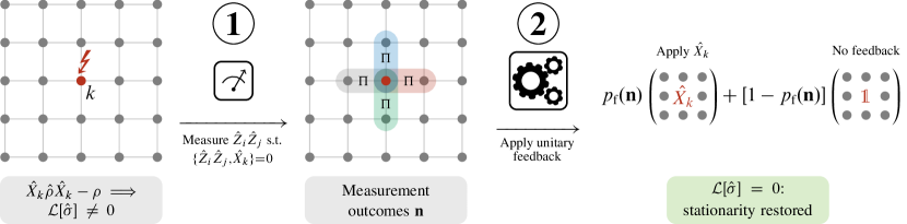
Figure 1: Schematic illustration of the measurement and feedback protocol for correcting incoherent errors in the Lindbladian that take the form of a Pauli $X$ operator. The desired steady state is $\sigma=\mathrm{e}^{-\Phi}$, where $\Phi$ corresponds to a 2D classical Ising model. In the presence of stray transverse fields, this state is no longer the steady state of the Lindbladian, $\mathcal{L}[\sigma]\neq 0$. By performing measurements of the stabilizers and probabilistic unitary feedback, the desired steady state $\sigma$ can be restabilized. The measurements occur at a rate that is proportional to the strength of the stray fields.

One of the simplest possible solutions to the above conditions on $\gamma_{xy}$ is given by

$$\gamma_{x}(\mathbf{n})=\gamma\left(|\mathbf{n}|\right)=\begin{cases}\gamma_{4}\,\mathrm{e}^{\mp 4\mu}&\text{ if }2-|\mathbf{n}|=\pm 2,\\ \gamma_{2}\,\mathrm{e}^{\mp 2\mu}&\text{ if }2-|\mathbf{n}|=\pm 1,\\ 0&\text{ otherwise,}\end{cases}$$ (127)

where $\gamma_{2}$ and $\gamma_{4}$ are nonnegative constants. Such dynamics corresponds to a canonical (continuous-time) Gibbs sampler, along the lines of, e.g., the classic Metropolis algorithm [94].

A slightly more interesting scenario arises if we consider that the system is instead subject to incoherent $X$ errors, which occur at some rate $g_{0}$. At the level of the Lindbladian description, $\mathcal{L}$ in Eq. (125) is modified to

$$\mathcal{L}(\rho)\to\mathcal{L}(\rho)+g_{0}\sum_{x}\left(X_{x}\rho X_{x}-\rho\right)\,.$$ (128)

If this perturbation is not corrected, the stationarity of $\sigma$ is broken. To maintain the stationarity of $\sigma$, we can perform measurements and feedback designed to perfectly cancel the effects of the perturbation (128). In other words, we can add some dynamics to (128) by measurements and feedback so that the dynamics become (125) with coefficients given by (127). Using the results of Sec. 4.4.2, we can perform the following protocol. For each site $x$, in a time step $\delta t$, measure the stabilizers on edges connecting to site $x$ with probability $g_{0}\left(\mathrm{e}^{8\mu}-1\right)\delta t$. After we get the measurement result $n_{xy}$ for each neighboring site $y$, apply $X_{x}$ with probability $\Lambda_{\mathbf{n}}$, where $\Lambda_{\mathbf{n}}|_{|\mathbf{n}|=3}=\left(\mathrm{e}^{4\mu}-1\right)/\left(\mathrm{e}^{8\mu}-1\right)$, $\Lambda_{\mathbf{n}}|_{|\mathbf{n}|=4}=1$ and all other $\Lambda_{\mathbf{n}}=0$. The resulting dynamics is

$$\mathcal{L}\to\mathcal{L}+g_{0}\sum_{x}\mathcal{D}\left[X_{x}\right]+\sum_{x,\mathbf{n}}g_{0}\left(\mathrm{e}^{8\mu}-1\right)\left(\Lambda_{\mathbf{n}}\,\mathcal{D}\left[X_{x}\Pi_{x}(\mathbf{n})\right]+\left(1-\Lambda_{\mathbf{n}}\right)\mathcal{D}\left[\Pi_{x}(\mathbf{n})\right]\right)\,.$$ (129)

Recall that projector $\Pi_{x}(\mathbf{n})$ is defined in (123). This amounts to measurements that are Poisson distributed in time, with a probability of applying feedback that depends on the outcomes of the measurements. The method is summarized in Table 1 and Figure 1. Mathematically, we have simply adjusted the choice of $\gamma_{2,4}$ in the Gibbs sampler (127) to be compatible with the presence of the unwanted error (128). This choice is not unique; here we have made the choice that leads to the smallest possible $\gamma_{2,4}$.

Measurement result	incoherent Pauli errors		Hamiltonian errors
	Probability	Feedback	Probability	Feedback
$|\mathbf{n}|=0$	$0$	N/A	$\mathrm{e}^{-8\mu}$	$\frac{1}{\sqrt{2}}(\mathrm{i}X_{x}-\mathds{1})$
$|\mathbf{n}|=1$	$0$	N/A	$(1-\mathrm{e}^{-4\mu})/(\mathrm{e}^{8\mu}-1)$	$\frac{1}{\sqrt{2}}(\mathrm{i}X_{x}-\mathds{1})$
$|\mathbf{n}|=2$	$0$	N/A	$0$	N/A
$|\mathbf{n}|=3$	$(\mathrm{e}^{4\mu}-1)/(\mathrm{e}^{8\mu}-1)$	$X_{x}$	$(\mathrm{e}^{4\mu}-1)/(\mathrm{e}^{8\mu}-1)$	$\frac{1}{\sqrt{2}}(\mathrm{i}X_{x}+\mathds{1})$
$|\mathbf{n}|=4$	$1$	$X_{x}$	$1$	$\frac{1}{\sqrt{2}}(\mathrm{i}X_{x}+\mathds{1})$

Table 1: Summary of protocols for correcting incoherent Pauli errors and Hamiltonian errors, discussed in Secs. 5.1.1 and 5.1.2, respectively: for each site $x$, in a time step $\delta t$, measure the 4 stabilizers that touch $x$ with probability $g_{0}\left(\mathrm{e}^{8\mu}-1\right)\delta t$ or $h_{0}\left(\mathrm{e}^{8\mu}-1\right)\delta t$. Next, apply feedback based on the measurement results as described in the table. The probability of applying feedback and the operators that need to be applied only depends on the number of $-1$ in the measurement results of the stabilizers $|\mathbf{n}|$.

If we think of the repetition code as storing a logical qubit, notice that a single $Z$ is a logical operator; therefore, in the presence of single-$Z$ errors, no quantum error correcting code exists. After all, in our formalism, adding $Z$ errors does not modify the steady state at all! We take this moment to remind the reader that protecting a steady state is not equivalent to protecting quantum information, as discussed in Sec. 4.5. To build a quantum error correcting code using this framework, one must also look for dynamics that “slowly mixes” between different sectors of logical operators.

Hamiltonian errors

If the Hamiltonian of the system is subjected to an $X$ field

$$H\to H-h_{0}\sum_{x}X_{x}\,,$$ (130)

an analogous sequence of measurements and unitary feedback can be applied to maintain stationarity of $\sigma$. We assume that $h_{0}>0$. According to Sec. 4.4.1, we can easily get the modifications we need to make $\sigma=\mathrm{e}^{-\Phi}$ stationary:

$$\mathcal{L}(\rho)\to\mathcal{L}(\rho)+\mathrm{i}h_{0}\sum_{x}\left[X_{x},\,\rho\right]+h_{0}\left(\mathrm{e}^{8\mu}-1\right)\sum_{\mathbf{x},|\mathbf{n}|\neq 2}\left(\Lambda_{\mathbf{n}}\,\mathcal{D}\left[U_{\mathbf{x}}(\mathbf{n})\Pi_{\mathbf{x}}(\mathbf{n})\right](\rho)+\left(1-\Lambda_{\mathbf{n}}\right)\mathcal{D}\left[\Pi_{\mathbf{x}}(\mathbf{n})\right](\rho)\right),$$ (131)

where

$$\Lambda_{\mathbf{n}}=\left|1-\mathrm{e}^{-4\mu\left(2-|\mathbf{n}|\right)}\right|/\left(\mathrm{e}^{8\mu}-1\right),$$ (132a)

$$U_{\mathbf{x}}(\mathbf{n})=\frac{1}{\sqrt{2}}\left(X_{\mathbf{x}}-\operatorname{sgn}\left(2-|\mathbf{n}|\right)\mathrm{i}\mathds{1}\right).$$ (132b)

The dissipative part can be generated by measurements and feedback: in time interval $\delta t$, measure the stabilizers with probability $h_{0}\left(\mathrm{e}^{8\mu}-1\right)\delta t$, then apply $U_{x}(\mathbf{n})$ with probability $\Lambda_{\mathbf{n}}$ based on the measurement result $\mathbf{n}$. The protocol is also summarized in Table 1.

Figure 2: We numerically simulate dynamics analogous to (131) for 1D systems of size $L=11$ sites and $\mu=\frac{1}{4}\log{2}$ and change the Hamiltonian error to $h\sum_{x}X_{x}$. The change of the correlation function $\langle Z_{x}Z_{x+r}\rangle$ for different $h/h_{0}$ with respect to its value at $h=h_{0}$, denoted $\langle Z_{x}Z_{x+r}\rangle_{0}$. The absolute values of the correlator $\langle Z_{x}Z_{x+r}\rangle_{0}$ for $r=1,2,3,4$ are, respectively, $0.172,0.030,0.005,0.001$.

One desirable property of our construction is that it, at least naively, gives rise to an experimentally detectable measurement-induced phase transition. To understand why, suppose that we study the dynamics on a square lattice at $\mu=\mu_{\mathrm{c}}$, where $\mu_{\mathrm{c}}$ is the (inverse) critical temperature of the 2D Ising model. At $h=h_{0}$ the dynamics sample from the Ising critical point, and thus result in critical fluctuations; at $h=\infty$ we do not detect long-range order. At $h=0$, where we only apply measurement and feedback, notice that the gate $U_{x}$ is Clifford. One picture for the dynamics comes from considering an initial product state in the $Z$ basis; the ensuing time evolution alternates between measurements of syndromes of the form $Z_{x}Z_{y}$ and the unitary gates $U_{x}$. However, because the syndromes are measured between pairs of qubits before any $U$s are applied, it is never possible for the set of qubits that are not in $Z$ eigenstates to be adjacent. Therefore, the system remains in a product state, albeit not necessarily in the $Z$-basis. As a consequence, all $ZZ$ correlation functions are effectively modeled by approximating that the state stays in a product state for all times, but after syndromes are measured there is only a 50% chance of modifying the state (via Pauli $X$) on that site. This adjustment does not change expectation values of the (products of) $Z$s. Hence $\langle Z_{x}Z_{y}\rangle$ must be identical at late times if $h=0$ and $h=h_{0}$. For other values of $h$, the most plausible scenario is therefore one in which there is criticality or long-range order for $h\in[0,h_{0}]$, and not outside of this domain. While we cannot exactly simulate this open system in 2D, direct application of time-evolution superoperator $\mathrm{e}^{\mathcal{L}t}$ on very small 1D systems suggests that this picture is correct: see Fig. 2. We therefore conjecture that our construction leads to an experimentally observable measurement-induced phase transition at $h=h_{0}$, where the experimentalist can simply measure the criticality in $\langle ZZ\rangle$ correlators to detect the transition. This statement holds assuming that the feedback rate is always the same; one can also simply tune through the thermal phase transition in the steady state, but in this situation the relative rates of error correction depending on the number of flipped syndromes change in a “complicated way,” such that the phase diagram is not a simple function of $h/h_{0}$.

Lastly, we remark that, although the feedback scheme in this problem is Clifford, and (at discrete time steps) the continuous Hamiltonian evolution also generates Clifford gates, it does not appear to be the case that classical simulations of a circuit approximation to our model could accurately reproduce the dynamics. Indeed, note that already when $h=0$, the Clifford feedback on its own prepares a critical state. Introducing any additional $X$-type errors on top of this dynamics should lead to a short-range-correlated phase in classical simulations, and yet we see that the critical state is also robust at $h=h_{0}$. The reason appears to be that the relative phases in the Clifford error correction tend to cancel the phases accumulated via continuous time evolution under the transverse field; this is precisely the kind of quantum effect that cannot be captured via Clifford simulation.

Measurement errors

In the previous example, where we corrected for Hamiltonian errors that took the form of a transverse field, we assumed that the syndromes can be measured perfectly. If the syndrome measurements are imperfect (intuitively because the experimenter reads out an incorrect syndrome measurement outcome, with a known error rate for such measurements), it is still possible to exactly identify the location of a measurement-induced phase transition by specifying $\Phi$ to be the critical Ising model. Such a construction can be thought of as a toy model for fault-tolerant passive error correction using memoryless local decoding.

Following Sec. 4.4.5, we can account for the imperfect syndrome measurements by modifying the effective Lindblad operator to be

$$\sum_{\sum\mathbf{n}\neq 0}\Lambda_{\mathbf{n}}\,\mathcal{D}\left[U_{x}(\mathbf{n})\Pi_{x}(\mathbf{n})\right] \to\sum_{\mathbf{n}^{\prime},\sum\mathbf{n}\neq 0}\Lambda_{\mathbf{n}}\,p(\mathbf{n}^{\prime}|\mathbf{n})\,\mathcal{D}\left[U_{x}(\mathbf{n})\Pi_{x}(\mathbf{n}^{\prime})\right]$$

$$\to\sum_{\sum\mathbf{n}\neq 0}\Lambda_{\mathbf{n}}^{\prime}\,\mathcal{D}\left[U_{x}(\mathbf{n})\Pi_{x}(\mathbf{n})\right],$$ (133)

where $p(\mathbf{n}^{\prime}|\mathbf{n})=q^{\Delta\mathbf{n}}\,(1-q)^{4-\Delta\mathbf{n}}$, $q$ is the error rate when measuring a single stabilizer and $\Delta\mathbf{n}$ is the number of measurement results that differ between $\mathbf{n}$ and $\mathbf{n}^{\prime}$. The second line of (5.1.3) comes after the cancellation of dynamics described in Sec. 4.4.5. In order to keep $\sigma$ stationary, we need to modify $\Lambda_{\mathbf{n}}$ to make the coefficient $\Lambda_{\mathbf{n}}^{\prime}$ match (132a). The modified coefficients $\Lambda_{\mathbf{n}}$, which represent the rate we apply feedback after measurements in the experiments, can be easily calculated numerically. For example, if we choose $\mu=\frac{1}{4}\log{2}$, demand that $\Lambda_{\mathbf{n}}=\Lambda(|\mathbf{n}|)$, and keep $U_{x}(\mathbf{n})$ fixed, $\Lambda(|\mathbf{n}|)$ as functions of $q$ is shown in Fig. 3(a), from which we observe that we need $q\lesssim 0.3$ to be able to fix the errors, otherwise some of the $\Lambda$ must be negative to maintain stationarity.

Note that from Fig. 3(a), we have $\max_{\mathbf{n}}{\Lambda_{\mathbf{n}}}>1$ for nonzero $q$. Since the interpretation of $\Lambda$ is the probability of applying feedback, we can modify (131) by replacing $\Lambda_{\mathbf{n}}$ with $\Lambda_{\mathbf{n}}/\max_{\mathbf{n}}\Lambda_{\mathbf{n}}$ and correspondingly rescale the measurement rate.

Figure 3: (a) The coefficients $\Lambda(|\mathbf{n}|)$ as functions of measurement error rate $q$ for Hamiltonian error correction (131) for 2D Ising model. We choose $\mu=\frac{1}{4}\log{2}$. (b) The coefficients $\Lambda\left(|\mathbf{n}|\right)$ as functions of error rate $q$ for incoherent Pauli error correction (129) for 2D Ising model. We choose $\gamma_{4}=2$, $\gamma_{2}=\mathrm{e}^{-2\mu}$ and $\mu=\frac{1}{4}\log{2}$.

Similarly, when we correct incoherent Pauli errors with (129), if we include the measurement errors, we can follow the same analysis as (5.1.3) to modify $\Lambda_{\mathbf{n}}$. If we simply require that $\Lambda_{\mathbf{n}}^{\prime}$ to be the same as (129), we find that $\Lambda\left(|\mathbf{n}|>2\right)$ we need would be the same as $\Lambda\left(|\mathbf{n}|>2\right)$ in Fig. 3(a). It seems that we again need $q\lesssim 0.3$ to fix the error for $\mu=\frac{1}{4}\log{2}$. However, since we can always add T-even dynamics (125) without changing the stationary state, it turns out that we can choose some nonzero $\gamma_{4}$ and $\gamma_{2}$ to increase the threshold of $q$. One example is shown in Fig. 3(b), from which we can see that the critical value of $q$ can be slightly greater than $0.3$.

Biased quantum walks

The error correction scheme for the Hamiltonian errors breaks time-reversal symmetry, as one can explicitly check. However, it is also of interest to break time-reversal symmetry in more “intuitive ways”: for example, breaking T but preserving PT, where P is spatial inversion symmetry. A simple motivating example already at the classical level is the addition of bias to the motion of a collection of particles (whose number is conserved) in one dimension: in this setting, the classical effective theory for particle density $\rho$ is modified from $\partial_{t}\rho=D\partial_{x}^{2}\rho+\cdots$ to $\partial_{t}\rho=\partial_{x}\left(a\rho+b\rho^{2}+\cdots+D\partial_{x}\rho+\cdots\right)$. Here the coefficients $a$ and $b$ break T, but preserve PT [13]. To achieve this type of qualitative correction to the long wavelength dynamics in a quantum setting, we must consider additional T-breaking modifications to the Lindblad operators of the previous subsection.

In the discussion that follows, we focus on one-dimensional spin-1/2 chains of length $L$ satisfying periodic boundary conditions. The stationary state $\sigma=\mathrm{e}^{-\Phi}$ with $\Phi=-\mu\sum_{x}Z_{x}Z_{x+1}$. We use configurations $\{s^{\,}_{1},\dots,s^{\,}_{L}\}$ to represent eigenstates of $\sigma$, where $s^{\,}_{x}\in\{\circ,\bullet\}$, which correspond to the eigenvalues $\{+1,-1\}$ of the stabilizer $Z_{x}Z_{x+1}$, respectively. Each stabilizer configuration corresponds to two spin configurations related by the Ising symmetry $\prod_{x}X_{x}$. For simplicity, we project onto the subspace in which $\prod_{x}X_{x}=+1$ and consider dynamics that remains in this subspace. We remark that the only states in this “Hilbert space” are those where the total number of $\bullet$ is even.

Classical T-odd dynamics

We first consider effectively classical T-odd dynamics that protect our desired steady state. Intuitively, one of the simplest T-odd classical dynamics is to transform states $|\cdots\circ\bullet\cdots\rangle\rightarrow|\cdots\bullet\circ\cdots\rangle$ in a translationally invariant way. Such dynamics will produce a biased drift of domain walls, and is exactly analogous to the classical biased random walk described in the introduction to this subsection. The density matrix $\sigma$ is still stationary because for each specific stabilizer configuration $\{s^{\,}_{1},\dots,s^{\,}_{L}\}$, the number of $\circ\bullet$ motifs is always the same as the number of $\bullet\circ$ [81], so the rate of probability outflow from a particular configuration is always equal to the rate of probability inflow. In Appendix A, we show how to systematically construct all translational invariant classical T-odd dynamics for 1D systems.

The Lindbladian of such dynamics realized exclusively by measurements and feedback can be

$$\mathcal{L}=\gamma_{0}\sum_{x}\ \mathcal{D}\left(\lvert\bullet\circ_{x}\rangle\langle\circ\bullet_{x}\rvert\right)+\mathcal{D}\left(\lvert\bullet\circ_{x}\rangle\langle\bullet\circ_{x}\rvert\right)+\mathcal{D}\left(\lvert\bullet\bullet_{x}\rangle\langle\bullet\bullet_{x}\rvert\right)\mathcal{D}\left(\lvert\circ\circ_{x}\rangle\langle\circ\circ_{x}\rvert\right),$$ (134)

where

$$\left|\bullet\circ_{x}\middle\rangle\middle\langle\circ\bullet_{x}\right| =\frac{1}{4}X_{x}\left(\mathds{1}+Z_{x-1}Z_{x}\right)\left(\mathds{1}-Z_{x}Z_{x+1}\right),$$ (135a)

$$\left|\bullet\circ_{x}\middle\rangle\middle\langle\bullet\circ_{x}\right| =\frac{1}{4}\left(\mathds{1}-Z_{x-1}Z_{x}\right)\left(\mathds{1}+Z_{x}Z_{x+1}\right),$$ (135b)

$$\left|\circ\circ_{x}\middle\rangle\middle\langle\circ\circ_{x}\right| =\frac{1}{4}\left(\mathds{1}+Z_{x-1}Z_{x}\right)\left(\mathds{1}+Z_{x}Z_{x+1}\right),$$ (135c)

$$\left|\bullet\bullet_{x}\middle\rangle\middle\langle\bullet\bullet_{x}\right| =\frac{1}{4}\left(\mathds{1}-Z_{x-1}Z_{x}\right)\left(\mathds{1}-Z_{x}Z_{x+1}\right)\,.$$ (135d)

Note that this dynamics does protect quantum coherence between $\lvert 000\rangle$ and $\lvert 111\rangle$, since the measurements and feedback only detect and correct relative bit flips between sites. However, because the quantum dynamics looks strictly classical in the basis of stabilizer eigenstates, we refer to it as classical T-odd dynamics. We identify any dynamics of stabilizer eigenvalues that cannot be mapped to classical Markov chains as quantum dynamics.

Quantum T-odd dynamics

Next, we consider quantum T-breaking dynamics that can produce a biased drift of domain walls across the system in a purely quantum manner; we also show that there is no classical model that captures the resulting drift of domain walls. For simplicity, we use $\lvert\alpha_{x}\rangle$ to represent states $\lvert\cdots\alpha\cdots\rangle$, where the “motif” $\alpha$ is the local configuration at position $x$. The dynamics produced by local jump operators with coefficient $\gamma_{\alpha\beta}^{\alpha^{\prime}\beta^{\prime}}$ is represented by $\lvert\alpha\rangle\langle\beta\rvert\rightarrow\left|\alpha^{\prime}\middle\rangle\middle\langle\beta^{\prime}\right|$, where the order of indices of $\gamma$ is the same as (36) and the index of position is neglected for now. We say state $\left|\alpha\middle\rangle\middle\langle\beta\right|$ and $\left|\alpha^{\prime}\middle\rangle\middle\langle\beta^{\prime}\right|$ are coupled if both $\gamma_{\alpha\beta}^{\alpha^{\prime}\beta^{\prime}}$ and $\gamma_{\alpha^{\prime}\beta^{\prime}}^{\alpha\beta}$ are nonzero, which is represented by $\left|\alpha\middle\rangle\middle\langle\beta\right|\rightleftharpoons\left|\alpha^{\prime}\middle\rangle\middle\langle\beta^{\prime}\right|$. The rough picture of the dynamics is that terms of the form $\lvert\circ\circ\bullet\rangle\langle\circ\bullet\circ\rvert\rightarrow\lvert\circ\bullet\circ\rangle\langle\bullet\circ\circ\rvert$ can move domain walls to the left, thus producing the biased drift of domain walls.

A schematic diagram of the dynamics is shown in Fig. 4: we first couple diagonal states with some off-diagonal states $\lvert\circ\circ\bullet\rangle\langle\circ\bullet\circ\rvert\rightleftharpoons\lvert\circ\circ\bullet\rangle\langle\circ\circ\bullet\rvert\rightleftharpoons\lvert\circ\bullet\circ\rangle\langle\circ\circ\bullet\rvert$ and $\lvert\circ\bullet\circ\rangle\langle\bullet\circ\circ\rvert\rightleftharpoons\lvert\bullet\circ\circ\rangle\langle\bullet\circ\circ\rvert\rightleftharpoons\lvert\bullet\circ\circ\rangle\langle\circ\bullet\circ\rvert$. We then add the dynamics $\lvert\circ\circ\bullet\rangle\langle\circ\bullet\circ\rvert\rightarrow\lvert\circ\bullet\circ\rangle\langle\bullet\circ\circ\rvert$ and $\lvert\circ\bullet\circ\rangle\langle\circ\circ\bullet\rvert\rightarrow\lvert\bullet\circ\circ\rangle\langle\circ\bullet\circ\rvert$ so that the domain walls are moving to the left. We also need to add some additional jump operators (diagonal terms to $\gamma_{ij}$) to keep the dynamics completely positive. The result is translationally invariant dynamics, all of which is moreover T-even with the crucial exception of the superposition drift. The transitions between the off-diagonal states effectively produce the classical dynamics $\lvert\circ\circ\bullet\rangle\langle\circ\circ\bullet\rvert\rightarrow\lvert\bullet\circ\circ\rangle\langle\bullet\circ\circ\rvert$ in a purely quantum way.

In order to keep $\sigma$ stationary, we can use the formalism developed in Appendix A to see that $\gamma_{\beta\beta}^{\alpha\alpha}=\gamma_{\alpha\alpha}^{\beta\beta}$ and $\gamma_{\alpha\alpha}^{\alpha\beta}=\gamma_{\beta\alpha}^{\alpha\alpha}$ should hold for any $\alpha$ and $\beta$. One example is:

$$\mathcal{L}^{\text{Q}}(\rho)=\sum_{x}\mathcal{L}_{x}^{\mathrm{Q}}(\rho) =\sum_{x}\ \mathcal{D}\left[\lvert\circ\circ\bullet_{x}\rangle\left(\langle\circ\circ\bullet_{x}\rvert+\langle\circ\bullet\circ_{x}\rvert\right)\right](\rho)+\mathcal{D}\left[\left(\lvert\circ\circ\bullet_{x}\rangle+\lvert\circ\bullet\circ_{x}\rangle\right)\langle\circ\circ\bullet_{x}\rvert\right](\rho)$$

$$+\mathcal{D}\left[\lvert\bullet\circ\circ_{x}\rangle\left(\langle\bullet\circ\circ_{x}\rvert+\langle\circ\bullet\circ_{x}\rvert\right)\right](\rho)+\mathcal{D}\left[\left(\lvert\bullet\circ\circ_{x}\rangle+\lvert\circ\bullet\circ_{x}\rangle\right)\langle\bullet\circ\circ_{x}\rvert\right](\rho)$$

$$+\mathcal{D}\left[\lvert\bullet\circ\circ_{x}\rangle\langle\bullet\circ\circ_{x}\rvert\right](\rho)+\mathcal{D}\left[\lvert\circ\circ\bullet_{x}\rangle\langle\circ\circ\bullet_{x}\rvert\right](\rho)$$

$$+\frac{1}{2}\,\left(\lvert\circ\bullet\circ_{x}\rangle\langle\circ\circ\bullet_{x}\rvert\,\rho\,\lvert\circ\bullet\circ_{x}\rangle\langle\bullet\circ\circ_{x}\rvert+\lvert\bullet\circ\circ_{x}\rangle\langle\circ\bullet\circ_{x}\rvert\,\rho\,\lvert\circ\circ\bullet_{x}\rangle\langle\circ\bullet\circ_{x}\rvert\right),$$ (136)

where we can express the domain-wall basis states above via

$$\left|\circ\bullet\circ_{x}\middle\rangle\middle\langle\circ\circ\bullet_{x}\right| =\frac{1}{8}X_{x+2}\left(\mathds{1}+Z_{x}Z_{x+1}\right)\left(\mathds{1}+Z_{x+1}Z_{x+2}\right)\left(\mathds{1}-Z_{x+2}Z_{x+3}\right)$$ (137a)

$$\left|\bullet\circ\circ_{x}\middle\rangle\middle\langle\circ\bullet\circ_{x}\right| =\frac{1}{8}X_{x+1}\left(\mathds{1}+Z_{x}Z_{x+1}\right)\left(\mathds{1}-Z_{x+1}Z_{x+2}\right)\left(\mathds{1}+Z_{x+2}Z_{x+3}\right)$$ (137b)

$$\left|\circ\circ\bullet_{x}\middle\rangle\middle\langle\circ\circ\bullet_{x}\right| =\frac{1}{8}\left(\mathds{1}+Z_{x}Z_{x+1}\right)\left(\mathds{1}+Z_{x+1}Z_{x+2}\right)\left(\mathds{1}-Z_{x+2}Z_{x+3}\right)$$ (137c)

$$\left|\bullet\circ\circ_{x}\middle\rangle\middle\langle\bullet\circ\circ_{x}\right| =\frac{1}{8}\left(\mathds{1}-Z_{x}Z_{x+1}\right)\left(\mathds{1}+Z_{x+1}Z_{x+2}\right)\left(\mathds{1}+Z_{x+2}Z_{x+3}\right)\,.$$ (137d)

Note that in (5.2.2), the first two lines produce the couplings between diagonal states and off-diagonal states, while the last line produces the dynamics $\lvert\circ\circ\bullet\rangle\langle\circ\bullet\circ\rvert\rightarrow\lvert\circ\bullet\circ\rangle\langle\bullet\circ\circ\rvert$ and $\lvert\circ\bullet\circ\rangle\langle\circ\circ\bullet\rvert\rightarrow\lvert\bullet\circ\circ\rangle\langle\circ\bullet\circ\rvert$, which is the only T-breaking part.

The effects of the quantum biased drift are shown in Fig. 4 (solid blue line): we numerically simulated this model in small one-dimensional systems with $\mu=\frac{1}{4}\log{2}$, and calculated correlation functions $\langle S_{x-1}(t)S_{x}(0)\rangle-\langle S_{x+1}(t)S_{x}(0)\rangle$ and $\langle O_{x-2}(t)O_{x}(0)\rangle-\langle O_{x+2}(t)O_{x}(0)\rangle$ for the dynamics (5.2.2), where $S_{x}=Z_{x}Z_{x+1}$ is the stabilizer, $O_{x}=\left|\bullet\circ_{x}\middle\rangle\middle\langle\circ\bullet_{x}\right|+\left|\circ\bullet_{x}\middle\rangle\middle\langle\bullet\circ_{x}\right|$ and $\langle A(t)B(0)\rangle\equiv\operatorname{Tr}\left[\mathrm{e}^{\mathcal{L}^{\dagger}t}(A)B\sigma\right]$. Both correlation functions are nonzero for the quantum dynamics.

Figure 4: (a) The dynamics of the biased quantum walks in the density matrix: the blue arrows represent the coupling between diagonal elements with off-diagonal elements; the yellow arrows represent the T-breaking dynamics between off-diagonal elements. (b) Plot of the correlation function $\langle S_{x-1}(t)S_{x}(0)\rangle-\langle S_{x+1}(t)S_{x}(0)\rangle$ for biased quantum walks (5.2.2) (solid blue line), where $S_{x}=Z_{x}Z_{x+1}$ denotes the stabilizer at position $x$. We plot the same correlation function for the corresponding classical dynamics (139) (orange line). We also plot the correlation function for dynamics with more phase damping (140). The correlation functions for quantum dynamics with $\alpha=2$ (dashed blue line) and $\alpha=4$ (dotted blue line) are reduced in magnitude and the classical dynamics (orange line) are not affected. (c) We plot a different correlation function $\langle O_{x-2}(t)O_{x}(0)\rangle-\langle O_{x+2}(t)O_{x}(0)\rangle$ for the biased quantum walks (5.2.2) (blue line) and the corresponding classical dynamics (139) (orange line), where $O_{x}=\left|\bullet\circ_{x}\middle\rangle\middle\langle\circ\bullet_{x}\right|+\left|\circ\bullet_{x}\middle\rangle\middle\langle\bullet\circ_{x}\right|$. The function $\langle O(t)O(0)\rangle$ captures the drift in domain wall superposition. Therefore, it vanishes identically for the classical dynamics.

We now argue that the dynamical system (5.2.2) is intrinsically quantum: namely, the T-odd part of this dynamics cannot be mapped to an effective classical dynamics even if we change the basis of the system. We can show, at a minimum, that if such a basis change exists, the basis change is nonlocal. This is because the T-odd Lindbladian in (5.2.2) locally protects $\sigma$: dynamics at any position $x$. Translation invariance is not needed for stationarity; indeed,

$$\mathcal{L}_{x}^{\mathrm{Q}}(\sigma)=0$$ (138)

for arbitrary position $x$. For classical dynamics, T-odd terms cannot be added locally in this manner while preserving stationarity, since T-odd classical dynamics only respect stationarity when they lead to biased flows around closed cycles in state space. More physically, if domain walls drift to the right only locally in region $R$, then they must “pile up” on the right-hand side of region $R$, in contradiction with the assertion that the same translation-invariant $\sigma$ exists for the locally modified chain. Therefore, if there exists a change of basis that would make the dynamics classical, $\mathcal{L}$ cannot be transformed to any local dynamics, and the classical dynamics would be highly nonlocal.

The difference between quantum and classical dynamics is also reflected in certain correlation functions. In Fig. 4, we depict the correlation function for classical dynamics (orange line)

$$\mathcal{L}^{\text{c}}(\rho)=\sum_{x}\ \mathcal{D}\left[\lvert\bullet\circ\circ_{x}\rangle\langle\circ\circ\bullet_{x}\rvert\right](\rho)+\mathcal{D}\left[\lvert\bullet\bullet\circ_{x}\rangle\langle\circ\bullet\bullet_{x}\rvert\right](\rho)\ ,$$ (139)

which also has the effect of moving domain walls to the left. The last term of the classical dynamics is needed to keep $\sigma$ stationary. From Fig. 4(b), the drifting for classical dynamics is much stronger than the quantum dynamics. However, in Fig. 4(c), as a correlation function that captures quantum effect, the correlation function $\langle O_{x-2}(t)O_{x}(0)-O_{x+2}(t)O_{x}(0)\rangle$, which captures the drift in domain wall superpositions, and hence vanishes identically for the classical dynamics. This constitutes additional evidence that the dynamics (5.2.2) is intrinsically quantum.

We can also demonstrate a quantum Zeno effect [105], in which rapidly increasing the rate of measurement will freeze out the bias in the quantum random walk dynamics. This is an intrinsically quantum phenomenon, so it will only exist for the quantum dynamics (5.2.2). We model a Zeno effect by increasing the coefficients of terms in the third line of the last equation in (5.2.2) by introducing the parameter $\alpha$, leading to

$$\mathcal{L}\rightarrow\mathcal{L}+\alpha\left(\mathcal{D}\left[\lvert\bullet\circ\circ_{x}\rangle\langle\bullet\circ\circ_{x}\rvert\right]+\mathcal{D}\left[\lvert\circ\circ\bullet_{x}\rangle\langle\circ\circ\bullet_{x}\rvert\right]\right)\,.$$ (140)

For the quantum dynamics, since the biased motion only comes from the last line of (5.2.2), which only couples off-diagonal terms, the motion of domain walls can be reduced in magnitude by the additional phase damping caused by (140). As shown in Fig. 4(b), We numerically simulated (140) with $\alpha=2$ or 4 and calculated the correlation function $\langle S_{x-1}(t)S_{x}(0)\rangle-\langle S_{x+1}(t)S_{x}(0)\rangle$ for both classical (orange line) and quantum dynamics (dashed blue line). The correlation function for quantum dynamics decreases when we increase $\alpha$, while for classical dynamics, the correlation function remains the same. This is further evidence that the $\alpha$-dependent term serves to suppress a fundamentally quantum-mechanical T-odd effect.

Conclusion

In this paper, we have described a systematic classification of the possible quantum open dynamical systems that protect a steady state $\sigma=\mathrm{e}^{-\Phi}$. When $\Phi$ could be expressed as a sum over commuting operators, we could further classify all possible few-body Lindbladians that protect $\sigma$ in a many-body setting, up to a handful of exceptions related to the classification of classical Markov chains with known steady state.

At the most mathematical level, our construction provides a significant generalization of the Davies Lindbladian, which drives a quantum system towards a Gibbs state ($\Phi=\beta H$). Unlike Davies’ Lindbladian, our protocols do not require that the system be driven by the same Hamiltonian as the steady state itself: this enables uniquely quantum mechanical phenomena in which the “drive” is counteracted by measurement and feedback. It is quite likely that, as in classical systems [42, 43], the non-Davies quantum Lindbladians discussed in this paper have a larger spectral gap, and thus prepare the desired state more quickly: indeed, recent work has used this idea [39, 40, 41].

At a slightly more practical level, our framework is naturally suited towards the problem of designing passive error correcting quantum codes; preliminary work along these lines is found in [102]. As we illustrated at length, our framework can describe the feedback schemes needed to stabilize a target state in the presence of quite generic errors. It is therefore possible to design targeted error-correcting protocols that are tuned towards hardware-specific error models and rates, including the highly-biased noise [106] that characterizes superconducting qubits, among other platforms. Using this framework, it may be possible to more systematically optimize over the space of possible code modifications to protect against biased error models, following [107]. Our approach naturally handles coherent noise as well, and may provide more optimized error correcting protocols than a general-purpose decoder. Such coherent noise is possible in both transmon qubits [108] as well as neutral atom qubits [109, 110].

At a more physical level, the methods developed in this paper represent a promising route towards engineering experimentally-detectable measurement-induced phase transitions, by designing particular feedback schemes that precisely compensate for known Hamiltonian “errors.” We have already presented one such example in Sec. 5, though we suspect that many more exist. Moreover, the formalism of this work may help to more systematically classify the possible phases of “active” quantum systems. For example, Ref. 111 argued that using measurement and feedback, it was possible to spontaneously break a continuous symmetry in one dimension, albeit with a protocol that was sensitive to noise. Intuitively, their protocol can be understood in our framework as the $\beta\to\infty$ limit of dynamics that protects the steady state

$$\Phi\sim-\beta\sum_{i}\mathbf{S}_{i}\cdot\mathbf{S}_{i+1}.$$ (141)

Since this Heisenberg model does not have long-range order in one spatial dimension, the conclusions of Ref. 111 are consistent with our framework’s expectations, in which adding a small amount of noise (taking $\beta$ finite) destabilizes the long-range order.

We should stress, at the same time, that while our methods are quite powerful at preparing desired quantum states, certain simple models of local classical or quantum dynamics are believed to have quite complex $\Phi$ [14, 112]. Our methods are effectively designed for models with simple $\Phi$. We cannot rule out the possibility that some quantum dynamical universality classes lie beyond the purview of our methods, precisely because they admit local Lindbladians with highly nonlocal $\Phi$. It remains an interesting problem to understand whether such models still admit some reasonable notion of a stable “phase of matter” [113], as well as to understand whether or not models with nonlocal $\Phi$ that do represent novel universality classes might be describable in our framework using a new set of degrees of freedom.

Lastly, we note that when $\Phi=\beta H$, a very powerful effective field theory based on a Schwinger-Keldysh path integral [77, 78, 79, 80] has been developed for studying quantum dissipative effective field theories. It would be fascinating if these methods can be generalized to the nonthermal dynamics described in this paper. One possible difficulty in achieving this goal will be that in any saddle point limit where such path integrals can be readily analyzed, nonthermal dynamics may already be largely, if not entirely, captured by a classical effective field theory developed in [13]. Such classical methods seem unlikely to capture all of the quantum coherent phenomena described in this work.

Appendix A Generating T-odd ${\gamma_{ab}}$ with ${c_{a}=c_{b}}$

Here we show how to generate T-odd dynamics of ${\gamma_{ab}}$ with ${c_{a}=c_{b}}$. For a general open quantum system, one can choose a basis $\{\lvert a\rangle\}$ that diagonalizes the stationary state ${\sigma=\sum_{a}\sigma_{a}\,\left|a\middle\rangle\middle\langle a\right|}$. Using jump operators ${F_{ab}=\left|a\middle\rangle\middle\langle b\right|}$, the Lindbladian can be written as

$$\mathcal{L}(\rho)= -\sum_{ab}\mathrm{i}\,h_{ab}\left[F_{ab},\,\rho\right]+\sum_{abcd}\gamma_{bd}^{ac}\left(F_{ab}\rho F_{cd}^{\dagger}-\frac{1}{2}\left\{F_{cd}^{\dagger}F_{ab},\,\rho\right\}\right).$$ (142)

In this language, the constraints imposed by stationarity can be separated into two parts,

$$\left\langle a\middle|\mathcal{L}[\sigma]\middle|a\right\rangle =\sum_{c}\left(\sigma_{c}\gamma_{cc}^{aa}-\sigma_{a}\gamma_{aa}^{cc}\right)=0,$$ (143a)

$$\left\langle a\middle|\mathcal{L}[\sigma]\middle|b\right\rangle =-\mathrm{i}(\sigma_{b}-\sigma_{a})h_{ab}+\sum_{c}\left[\sigma_{c}\gamma_{cc}^{ab}-\frac{1}{2}(\sigma_{a}+\sigma_{b})\gamma_{ba}^{cc}\right]=0,\;a\neq b.$$ (143b)

In (143a), the diagonal part of the ${\gamma}$ matrix, ${\gamma_{cc}^{aa}}$ represents the transition rate of ${\left|c\middle\rangle\middle\langle c\right|\rightarrow\left|a\middle\rangle\middle\langle a\right|}$, which include all the dynamics between the diagonal part of ${\sigma}$. This part of dynamics can be mapped to classical Markov chains, so we will refer to them as the classical part of dynamics. The off-diagonal part of the ${\gamma}$ matrix that appears in (143b), ${\gamma_{cc}^{ab}}$ and ${\gamma_{ba}^{cc}}$ can be roughly understood as the transition rate of ${\left|c\middle\rangle\middle\langle c\right|\rightarrow\left|a\middle\rangle\middle\langle b\right|}$ and ${\left|b\middle\rangle\middle\langle a\right|\rightarrow\left|c\middle\rangle\middle\langle c\right|}$, which will be referred to as the quantum part of dynamics. Note that the coefficients $\gamma^{ab}_{cd}$, where all the indices are different, are also in the quantum part. These coefficients are not constrained by the stationarity of $\sigma$. The only constraint for them is the positivity of $\gamma$.

The constraints of the classical dynamics (143a) seem hard to solve in complete generality. Each variable ${\gamma_{cc}^{aa}}$ appears in two different equations which cannot be neatly decoupled from the rest. It can formally be solved by finding all cycles in the state space and attempting to add nonzero transition rates that cause the system to flow around each cycle in a biased way. However, such biased “random walks” are directly in the many-body state space, so they do not generically correspond to local Lindbladians. However, as we will show shortly, we know how to generate 1D translationally invariant local classical dynamics for systems with $\sigma=\text{e}^{-\Phi}$ in the form of Eq. (53) [114].

The quantum part of the constraints is easier: each variable only appears once. For many-body systems, even with the constraints of locality, we only need to solve a finite number of equations for each variable, so a complete solution can be found, including when restricting to local dynamics.

In summary, therefore, we will systematically show in this appendix how to classify all 1D translationally invariant classical T-odd dynamics and all quantum dynamics.

We now explicitly show how to generate these dynamics, starting with a simple example before moving on to the general case. Consider a 1D spin-1/2 chain with length $L$ and periodic boundary conditions (PBCs) $x+L\cong x$ for any site $x$. We take the stationary state $\sigma\propto\exp\left(\,\mu\sum_{x}Z_{x}\right)$, and use $\lvert s\rangle$ to represent a configuration $\{s^{\,}_{1},\dots,s^{\,}_{L}\}$, where $s^{\,}_{x}\in\{-1,1\}$ is the eigenvalue of the stabilizer $Z_{x}$. $\sigma=\sigma_{ss^{\prime}}\lvert s\rangle\langle s^{\prime}\rvert$ is diagonal with the basis $\{\lvert s\rangle\}$, so (as above) the transitions between density matrices $|s\rangle\langle s|$ and $|s^{\prime}\rangle\langle s^{\prime}|$ is defined to be the classical dynamics. Since we want local dynamics, we only consider $q$-body spatially local jump operators, namely transitions that take $|s\rangle\langle s|$ to $|s^{\prime}\rangle\langle s^{\prime}|$ when $s$ and $s^{\prime}$ differ on at most $q$ adjacent sites, e.g. $s=s_{1\cdots x-1}\otimes\alpha_{x\cdots x+q-1}\otimes s_{x+q\cdots L}$ and $s^{\prime}=s_{1\cdots x-1}\otimes\alpha^{\prime}_{x\cdots x+q-1}\otimes s_{x+q\cdots L}$. In the remainder of this appendix, we will use “$\alpha$” to denote the motif (of length $\leq q$) sites on which two related microstates differ. Similar to (55), we choose the jump operators to be

$$A_{\beta\alpha,x}=\mathds{1}_{1\cdots x-1}\otimes|\beta\rangle\langle\alpha|_{x\cdots x+q-1}\otimes\mathds{1}_{x+q\cdots L}.$$ (144)

where we remind the reader that $\alpha,\beta$ denote motifs of $q$ adjacent stabilizer eigenvalues in the local 1D chain. In this appendix, the $\alpha\beta$ notation will be easier to understand than the notation in (55). We define

$$c_{\beta\alpha,x}=\exp\left[\mu\sum_{y=x}^{x+q-1}\frac{\beta_{y}-\alpha_{y}}{2}\right]$$ (145)

for use in what follows. With these jump operators, a general $q$-local Lindbladian can be written as

$$\mathcal{L}(\rho)= -\mathrm{i}\left[H,\,\rho\right]+\sum_{\alpha\beta\alpha^{\prime}\beta^{\prime},x}\gamma_{\beta\beta^{\prime},x}^{\alpha\alpha^{\prime}}\left(\lvert\alpha^{x}\rangle\langle\beta^{x}\rvert\,\rho\,\lvert\beta^{\prime x}\rangle\langle\alpha^{\prime x}\rvert-\frac{1}{2}\left\{\langle\alpha^{\prime x}|\alpha^{x}\rangle\,\lvert\beta^{\prime x}\rangle\langle\beta^{x}\rvert,\,\rho\right\}\right).$$ (146)

We now discuss the “classical part of dynamics”, which was defined to only depend on coefficients $\gamma_{\beta\beta,x}^{\alpha\alpha}$ which takes a diagonal density matrix to another one. Strictly speaking, there can also be “quantum” dynamics if the dots in the kets and bras are (not) the same: namely, the classical dynamics will always be accompanied by some quantum dynamics because of locality. However, since these quantum dynamics would not affect the stationarity criterion, we will not discuss them further, and focus on the truly classical dynamics which is constrained by stationarity.

Let us assume translation invariance, so that $\gamma_{\beta\beta,x}^{\alpha\alpha}=\gamma_{\beta\beta}^{\alpha\alpha}$ is independent of the position $x$. We will shortly see why this restriction is very helpful. Then the stationarity of ${\sigma}$ requires that for each configuration $\lvert s\rangle$,

$$\frac{\text{d}\sigma_{ss}}{\text{d}t} =\sigma_{ss}\left(\sum_{\beta\alpha}N_{\beta}^{s}\,c_{\beta\alpha}^{2}\gamma^{\beta\beta}_{\alpha\alpha}-\sum_{\beta\alpha}N_{\beta}^{s}\gamma_{\beta\beta}^{\alpha\alpha}\right)=\sigma_{ss}\sum_{\alpha}N_{\beta}^{s}f_{\beta}=0,$$ (147)

where $N_{\beta}^{s}$ is the number of motif $\beta$ in the microstate $s$. In the second equation above, the first term denotes the number of classical configurations entering $|s\rangle\langle s|$ and the second term denotes the rate at which the system decays out of $|s\rangle\langle s|$. The function $f$ is defined as

$$f_{\beta}=\sum_{\alpha}\left(c_{\beta\alpha}^{2}\gamma^{\beta\beta}_{\alpha\alpha}-\gamma_{\beta\beta}^{\alpha\alpha}\right),$$ (148)

which is a function that only depends on the motif $\beta$. If we can find all possible functions ${f}$ that satisfy

$$\sum_{\alpha}N_{\alpha}^{s}f_{\alpha}=0$$ (149)

for all configurations, we can then solve for all possible $\gamma_{\alpha\alpha}^{\beta\beta}$ out of the function $f$, which include all classical dynamics.

One can prove [114] that all solutions $f$ to (149) can be written as

$$f_{\alpha}=g\left(\alpha_{1},\dots,\alpha_{q-1}\right)-g\left(\alpha_{2},\dots,\alpha_{q}\right)\,,~{}~{}$$ (150)

where $g$ is an arbitrary function and ${\{\alpha_{1},\cdots,\alpha_{q}\}}$ is the motif $\alpha$, and that there are $2^{q-1}-1$ nontrivial linearly independent choices of function $g$. The latter claim follows transparently from counting all possible linearly independent functions on $\mathbb{Z}_{2}^{q-1}$ (noting that $g=1$ does not contribute to $f_{\alpha}$); the former claim follows, in part, from the observation that the linear relation (149) fails in generality if $f_{\alpha}$ has any term proportional to $\alpha_{1}\alpha_{q}$. From (150), we can get all possible $f$ functions and all possible classical dynamics. Note that this part of the dynamics can always be generated by measuring stabilizers and applying feedback, possibly after adding additional dissipative terms to the Lindbladian (that protect $\sigma$).

These dynamics can be generalized to systems with stationary states $\sigma\propto\exp\left(\sum_{x}\mu_{x}Z_{x}\right)$. In (148), if we take into account the position of the coefficients $\gamma_{P\bar{\alpha},x}^{P\bar{\alpha}}$ and $\gamma_{P\alpha,x}^{P\alpha}$, we find that coefficients with different $x$ don’t appear in the same equation. Therefore, we can keep function $f$ unchanged and demand that for every $x$,

$$f_{\beta}=\sum_{\alpha}\left(c_{\beta\alpha,x}^{2}\gamma^{\beta\beta}_{\alpha\alpha,x}-\gamma_{\beta\beta,x}^{\alpha\alpha}\right).$$ (151)

Unfortunately, we have found it very challenging to generalize this method beyond one dimensional lattice graphs. We do remark, however, that the above method easily generalizes to models where the stabilizers act on multiple sites, as in Section 5.2.2.

Now we discuss the quantum part of the constraints. Here, we will not need to assume that some aspect of the dynamics is translationally invariant. Still, for simplicity we will mainly focus on $\sigma\propto\exp\left(\mu\sum_{x}Z_{x}\right)$, as the generalization is direct. The constraints of quantum dynamics come from (143b), where we can regard $\lvert a\rangle$ and $\lvert b\rangle$ as specific configurations. From (94), we can always find a Hamiltonian to counteract the effects of $\gamma_{ab}$ whenever $c_{a}\neq c_{b}$, and so the classification problem becomes trivial: $\langle a|H|b\rangle$ is whatever is needed to obey (94). Notice that as discussed in the main text, locality will be respected. Hence, we only need to focus on the case where $c_{a}=c_{b}$. With $q$-local dynamics, only when $\lvert a\rangle$ and $\lvert b\rangle$ differ by $\leq q$ adjacent sites:

$$|a\rangle =|s\rangle_{1\cdots x-1}\otimes|\alpha\rangle_{x\cdots x+q-1-n}\otimes|s^{\prime}\rangle_{x+q-n\cdots L}$$ (152a)

$$|b\rangle =|s\rangle_{1\cdots x-1}\otimes|\beta\rangle_{x\cdots x+q-1-n}\otimes|s^{\prime}\rangle_{x+q-n\cdots L},$$ (152b)

can the coefficients on the RHS of (143b) can be nonzero. Notice that we can take $0\leq n\leq q-1$. For each pair of $n$, $x$, $\alpha$ and $\beta$, we obtain a decoupled set of $4^{n}$ equations to solve (this counting assumes the stabilizers take values $\pm 1$). For the simplest case of $n=0$, we get a single equation to solve:

$$\frac{\text{d}\sigma_{ab}}{\text{d}t} =\sum_{s}\left(\sigma_{ss}\gamma_{ss}^{ab}-\frac{1}{2}(\sigma_{aa}+\sigma_{bb})\gamma_{ba}^{ss}\right)=\sigma_{aa}\sum_{\gamma}\left(c_{\gamma\alpha}^{2}\,\gamma^{\alpha\beta}_{\gamma\gamma,x}-\gamma^{\gamma\gamma}_{\beta\alpha,x}\right)=0.$$ (153)

Note that $\sigma_{aa}=\sigma_{bb}$ because we only discuss dynamics of $\gamma_{ab}$ with $c_{a}=c_{b}$. Due to spatial locality, this constraint does not depend on $|s\rangle$ or $|s^{\prime}\rangle$ in (152). Lastly, there is no other equation that constrains $\gamma^{\alpha\beta}_{\gamma\gamma,x}$ or $\gamma^{\gamma\gamma}_{\beta\alpha,x}$: the sole constraint on these matrix elements is (153).

If $n>0$, things are a little more complicated: the $q$-site jump operator can be of the form $A_{\gamma\delta,y}$ for $x-n\leq y\leq x$. We can solve for the resulting constraints on $\gamma$s as follows: consider the states:

$$|\tilde{a}(r,r^{\prime})\rangle =|s\rangle_{1\cdots x-1-n}\otimes|r\rangle_{x-n\cdots x-1}\otimes|\alpha\rangle_{x\cdots x+q-1-n}\otimes|r^{\prime}\rangle_{x+q-n\cdots x+q-1}\otimes|s^{\prime}\rangle_{x+q\cdots L}$$ (154a)

$$|\tilde{b}(r,r^{\prime})\rangle =|s\rangle_{1\cdots x-1-n}\otimes|r\rangle_{x-n\cdots x-1}\otimes|\beta\rangle_{x\cdots x+q-1-n}\otimes|r^{\prime}\rangle_{x+q-n\cdots x+q-1}\otimes|s^{\prime}\rangle_{x+q\cdots L},$$ (154b)

where here $|r\rangle$ and $|r^{\prime}\rangle$ are again identical between $|\tilde{a}\rangle$ and $|\tilde{b}\rangle$. We must now consider the $4^{n}$ equations that arise from evaluating $\langle\tilde{a}(r,r^{\prime})|\mathcal{L}[\sigma]|\tilde{b}(r,r^{\prime})\rangle$. There is not an elegant notation to express the general form of these constraints, but we can illustrate their form with a simple example that straightforwardly generalizes. Consider the simplest nontrivial case of $q=2$ and $n=1$, where $|\alpha\rangle=|0\rangle$ and $|\beta\rangle=|1\rangle$, and $x=2$. Analogous to (153), we find a set of 4 constraints:

$$\sum_{k,k^{\prime}=0,1}\left[c_{(kk^{\prime})(r0),1}^{2}\gamma_{(kk^{\prime})(kk^{\prime}),1}^{(r0)(r1)}-\gamma^{(kk^{\prime})(kk^{\prime})}_{(r1)(r0),1}+c_{(kk^{\prime})(0r^{\prime}),2}^{2}\gamma_{(kk^{\prime})(kk^{\prime}),2}^{(0r^{\prime})(1r^{\prime})}-\gamma^{(kk^{\prime})(kk^{\prime})}_{(1r^{\prime})(0r^{\prime}),2}\right]=0$$ (155)

for $r,r^{\prime}=0,1$. Notice that these equations are not all independent, since e.g. the last term in the above equation is independent of the value of $r$. It is tedious, but straightforward, to generalize this construction to general $n$ and $q$.

For systems with stabilizers that introduce degeneracy, so long as the operators that transition between such states (e.g. logical operators in an error correcting code) are nonlocal, the existence of such degeneracy does not modify the discussion above. Therefore, for systems with stationary states $\sigma=\exp\left(-\Phi\right)$ in the form of (53), we can get all possible quantum dynamics of $\gamma_{ab}$ with $c_{a}=c_{b}$ by solving the generalizations of (153) and (155). In contrast, for the dynamics of $\gamma_{ab}$ with $c_{a}=c_{b}$, we can only classify 1D classical T-odd dynamics with translation invariance.

References

- [1] K. G. Wilson, Renormalization group and critical phenomena. I. Renormalization group and the Kadanoff scaling picture, Phys. Rev. B 4, 3174 (1971), doi:10.1103/PhysRevB.4.3174.
- [2] K. G. Wilson, Renormalization group and critical phenomena. ii. phase-space cell analysis of critical behavior, Phys. Rev. B 4, 3184 (1971), doi:10.1103/PhysRevB.4.3184.
- [3] S. Ramaswamy, The mechanics and statistics of active matter, Ann. Rev. Cond. Mat. Phys. 1(1), 323 (2010), doi:10.1146/annurev-conmatphys-070909-104101.
- [4] M. C. Marchetti, J. F. Joanny, S. Ramaswamy, T. B. Liverpool, J. Prost, M. Rao and R. A. Simha, Hydrodynamics of soft active matter, Rev. Mod. Phys. 85, 1143 (2013), doi:10.1103/RevModPhys.85.1143.
- [5] S. Ramaswamy, Active matter, J. Stat. Mech. Theor. Exp. 2017(5), 054002 (2017), doi:10.1088/1742-5468/aa6bc5.
- [6] K. Adachi, K. Takasan and K. Kawaguchi, Activity-induced phase transition in a quantum many-body system, Phys. Rev. Res. 4, 013194 (2022), doi:10.1103/PhysRevResearch.4.013194.
- [7] R. Khasseh, S. Wald, R. Moessner, C. A. Weber and M. Heyl, Active quantum flocks (2023), 2308.01603.
- [8] M. Yamagishi, N. Hatano and H. Obuse, Defining a quantum active particle using non-Hermitian quantum walk (2023), 2305.15319.
- [9] F. Verstraete, M. M. Wolf and J. Ignacio Cirac, Quantum computation and quantum-state engineering driven by dissipation, Nature Phys. 5(9), 633 (2009).
- [10] S. B. Bravyi and A. Y. Kitaev, Quantum codes on a lattice with boundary (1998), quant-ph/9811052.
- [11] A. G. Fowler, M. Mariantoni, J. M. Martinis and A. N. Cleland, Surface codes: Towards practical large-scale quantum computation, Physical Review A 86(3) (2012), doi:10.1103/physreva.86.032324.
- [12] M. B. Hastings, Topological order at nonzero temperature, Phys. Rev. Lett. 107, 210501 (2011), doi:10.1103/PhysRevLett.107.210501.
- [13] X. Huang, J. H. Farrell, A. J. Friedman, I. Zane, P. Glorioso and A. Lucas, Generalized time-reversal symmetry and effective theories for nonequilibrium matter (2023), 2310.12233.
- [14] D. Roberts, A. Lingenfelter and A. Clerk, Hidden time-reversal symmetry, quantum detailed balance and exact solutions of driven-dissipative quantum systems, PRX Quantum 2, 020336 (2021), doi:10.1103/PRXQuantum.2.020336.
- [15] B. Skinner, J. Ruhman and A. Nahum, Measurement-induced phase transitions in the dynamics of entanglement, Phys. Rev. X 9, 031009 (2019), doi:10.1103/PhysRevX.9.031009.
- [16] Y. Li, X. Chen and M. P. A. Fisher, Quantum zeno effect and the many-body entanglement transition, Phys. Rev. B 98, 205136 (2018), doi:10.1103/PhysRevB.98.205136.
- [17] A. Chan, R. M. Nandkishore, M. Pretko and G. Smith, Unitary-projective entanglement dynamics, Phys. Rev. B 99, 224307 (2019), doi:10.1103/PhysRevB.99.224307.
- [18] Y. Li, X. Chen and M. P. A. Fisher, Measurement-driven entanglement transition in hybrid quantum circuits, Phys. Rev. B 100, 134306 (2019), doi:10.1103/PhysRevB.100.134306.
- [19] S. Choi, Y. Bao, X.-L. Qi and E. Altman, Quantum error correction in scrambling dynamics and measurement-induced phase transition, Phys. Rev. Lett. 125, 030505 (2020), doi:10.1103/PhysRevLett.125.030505.
- [20] C.-M. Jian, Y.-Z. You, R. Vasseur and A. W. W. Ludwig, Measurement-induced criticality in random quantum circuits, Phys. Rev. B 101, 104302 (2020), doi:10.1103/PhysRevB.101.104302.
- [21] S. Roy, J. T. Chalker, I. V. Gornyi and Y. Gefen, Measurement-induced steering of quantum systems, Phys. Rev. Res. 2, 033347 (2020), doi:10.1103/PhysRevResearch.2.033347.
- [22] Y. Herasymenko, I. Gornyi and Y. Gefen, Measurement-driven navigation in many-body Hilbert space: Active-decision steering (2022), 2111.09306.
- [23] T. Iadecola, S. Ganeshan, J. H. Pixley and J. H. Wilson, Dynamical entanglement transition in the probabilistic control of chaos (2022), 2207.12415.
- [24] M. Buchhold, T. Müller and S. Diehl, Revealing measurement-induced phase transitions by preselection (2022), 2208.10506.
- [25] E. Chertkov, Z. Cheng, A. C. Potter, S. Gopalakrishnan, T. M. Gatterman, J. A. Gerber, K. Gilmore, D. Gresh, A. Hall, A. Hankin, M. Matheny, T. Mengle et al., Characterizing a nonequilibrium phase transition on a quantum computer (2022), 2209.12889.
- [26] A. Milekhin and F. K. Popov, Measurement-induced phase transition in teleportation and wormholes (2023), 2210.03083.
- [27] A. J. Friedman, O. Hart and R. Nandkishore, Measurement-induced phases of matter require feedback, PRX Quantum 4, 040309 (2023), doi:10.1103/PRXQuantum.4.040309.
- [28] J. Y. Lee, W. Ji, Z. Bi and M. P. A. Fisher, Decoding measurement-prepared quantum phases and transitions: from Ising model to gauge theory, and beyond (2022), 2208.11699.
- [29] D. M. Greenberger, M. A. Horne and A. Zeilinger, Going beyond Bell’s theorem, In Bell’s theorem, quantum theory and conceptions of the universe, pp. 69–72. Springer (1989).
- [30] C. L. Degen, F. Reinhard and P. Cappellaro, Quantum sensing, Rev. Mod. Phys. 89, 035002 (2017), doi:10.1103/RevModPhys.89.035002.
- [31] A. R. Calderbank and P. W. Shor, Good quantum error-correcting codes exist, Physical Review A 54(2), 1098 (1996), doi:10.1103/physreva.54.1098.
- [32] A. Steane, Multiple-particle interference and quantum error correction, Proceedings of the Royal Society of London. Series A: Mathematical, Physical and Engineering Sciences 452(1954), 2551 (1996), doi:10.1098/rspa.1996.0136.
- [33] R. P. Feynman, Simulating physics with computers, International Journal of Theoretical Physics 21(6), 467 (1982).
- [34] S. Lee, J. Lee, H. Zhai, Y. Tong, A. M. Dalzell, A. Kumar, P. Helms, J. Gray, Z.-H. Cui, W. Liu et al., Evaluating the evidence for exponential quantum advantage in ground-state quantum chemistry, Nature Commun. 14(1), 1952 (2023).
- [35] C.-F. Chen, M. J. Kastoryano, F. G. Brandão and A. Gilyén, Quantum thermal state preparation, arXiv preprint arXiv:2303.18224 (2023).
- [36] K. Temme, T. J. Osborne, K. G. Vollbrecht, D. Poulin and F. Verstraete, Quantum metropolis sampling, Nature 471(7336), 87 (2011).
- [37] O. Shtanko and R. Movassagh, Algorithms for Gibbs state preparation on noiseless and noisy random quantum circuits, doi:10.48550/ARXIV.2112.14688 (2021).
- [38] P. Rall, C. Wang and P. Wocjan, Thermal state preparation via rounding promises, Quantum 7, 1132 (2023).
- [39] C.-F. Chen, M. J. Kastoryano and A. Gilyén, An efficient and exact noncommutative quantum Gibbs sampler (2023), 2311.09207.
- [40] C. Rouzé, D. S. França and A. M. Alhambra, Efficient thermalization and universal quantum computing with quantum Gibbs samplers (2024), 2403.12691.
- [41] Z. Ding, B. Li and L. Lin, Efficient quantum Gibbs samplers with Kubo–Martin–Schwinger detailed balance condition (2024), 2404.05998.
- [42] E. P. Bernard, W. Krauth and D. B. Wilson, Event-chain monte carlo algorithms for hard-sphere systems, Phys. Rev. E 80, 056704 (2009), doi:10.1103/PhysRevE.80.056704.
- [43] H. Suwa and S. Todo, Markov chain monte carlo method without detailed balance, Phys. Rev. Lett. 105, 120603 (2010), doi:10.1103/PhysRevLett.105.120603.
- [44] M. Doi, Second quantization representation for classical many-particle system, J. Phys. A: Math. Gen. 9(9), 1465 (1976), doi:10.1088/0305-4470/9/9/008.
- [45] M. Doi, Stochastic theory of diffusion-controlled reaction, J. Phys. A: Math. Gen. 9(9), 1479 (1976), doi:10.1088/0305-4470/9/9/009.
- [46] Peliti, L., Path integral approach to birth-death processes on a lattice, J. Phys. France 46(9), 1469 (1985), doi:10.1051/jphys:019850046090146900.
- [47] L. Peliti, Renormalisation of fluctuation effects in the A+A to A reaction, J. Phys. A: Math. Gen. 19(6), L365 (1986), doi:10.1088/0305-4470/19/6/012.
- [48] L. Kadanoff, Statistical Physics: Statics, Dynamics and Renormalization, World Scientific, ISBN 9789810237646 (2000).
- [49] P. Langevin, Sur la théorie du mouvement brownien, C. R. Acad. Sci. (Paris) 146, 530 (1908).
- [50] A. D. Fokker, Die mittlere Energie rotierender elektrischer Dipole im Strahlungsfeld, Annalen der Physik 348(5), 810 (1914), doi:https://doi.org/10.1002/andp.19143480507.
- [51] M. Planck, Über einen Satz der statistischen Dynamik und seine Erweiterung in der Quantentheorie, Sitzungsberichte der Königlich-Preussischen Akademie der Wissenschaften zu Berlin. Reimer (1917).
- [52] A. Kolmogorov, Über die analytischen Methoden in der Wahrscheinlichkeitsrechnung, Mathematische Annalen 104(1), 415 (1931), doi:10.1007/BF01457949.
- [53] F. Kelly, Reversibility and Stochastic Networks, Probability and Statistics Series. Wiley, ISBN 9780471276012 (1979).
- [54] G. Lindblad, Entropy, information and quantum measurements, Commun. Math. Phys. 33, 305 (1973), doi:10.1007/BF01646743.
- [55] G. Lindblad, On the generators of quantum dynamical semigroups, Commun. Math. Phys. 48(2), 119 (1976), doi:10.1007/BF01608499.
- [56] V. Gorini, A. Kossakowski and E. C. G. Sudarshan, Completely positive dynamical semigroups of N-level systems, Journal of Mathematical Physics 17(5), 821 (1976).
- [57] C. W. Gardiner and P. Zoller, Quantum Noise, Springer Series in Synergetics. Springer, 3 edn., ISBN 978-3-540-22301-6 (2004).
- [58] M. A. Nielsen and I. L. Chuang, Quantum Computation and Quantum Information: 10th Anniversary Edition, Cambridge University Press, doi:10.1017/CBO9780511976667 (2010).
- [59] C. A. Brasil, F. F. Fanchini and R. d. J. Napolitano, A simple derivation of the Lindblad equation, Revista Brasileira de Ensino de Física 35, 01 (2013), doi:10.1590/S1806-11172013000100003.
- [60] A. J. Daley, Quantum trajectories and open many-body quantum systems, Adv. Phys. 63(2), 77 (2014), doi:10.1080/00018732.2014.933502.
- [61] J. P. Garrahan, Aspects of nonequilibrium in classical and quantum systems: Slow relaxation and glasses, dynamical large deviations, quantum nonergodicity, and open quantum dynamics, Physica A 504, 130 (2018), doi:10.1016/j.physa.2017.12.149.
- [62] F. Thompson and A. Kamenev, Field theory of many-body Lindbladian dynamics, Annals Phys. 455, 169385 (2023), doi:10.1016/j.aop.2023.169385, 2301.02953.
- [63] K. Kraus, States, Effects, and Operations. Fundamental Notions of Quantum Theory., Lecture Notes in Physics. Springer Berlin, Heidelberg, Germany, ISBN 978-3-540-12732-1, doi:https://doi.org/10.1007/3-540-12732-1 (1983).
- [64] S. Diehl, A. Micheli, A. Kantian, B. Kraus, H. Büchler and P. Zoller, Quantum states and phases in driven open quantum systems with cold atoms, Nature Phys. 4(11), 878 (2008).
- [65] B. Kraus, H. P. Büchler, S. Diehl, A. Kantian, A. Micheli and P. Zoller, Preparation of entangled states by quantum Markov processes, Phys. Rev. A 78, 042307 (2008), doi:10.1103/PhysRevA.78.042307.
- [66] F. Fagnola and V. Umanità, Detailed balance, time reversal, and generators of quantum Markov semigroups, Math. Notes 84(1), 108 (2008), doi:10.1134/S0001434608070092.
- [67] F. Fagnola and V. Umanità, Generators of KMS symmetric Markov semigroups on symmetry and quantum detailed balance, Commun. Math. Phys. 298(2), 523 (2010), doi:10.1007/s00220-010-1011-1.
- [68] E. A. Carlen and J. Maas, Gradient flow and entropy inequalities for quantum Markov semigroups with detailed balance, J. Funct. Anal 273(5), 1810 (2017), doi:https://doi.org/10.1016/j.jfa.2017.05.003.
- [69] A. Romero-Bermúdez, K. Schalm and V. Scopelliti, Regularization dependence of the OTOC. Which Lyapunov spectrum is the physical one?, JHEP 07, 107 (2019), doi:10.1007/JHEP07(2019)107, 1903.09595.
- [70] X. Chen, Y. Gu and A. Lucas, Many-body quantum dynamics slows down at low density, SciPost Phys. 9, 071 (2020), doi:10.21468/SciPostPhys.9.5.071.
- [71] E. B. Davies, Markovian master equations, Commun. Math. Phys. 39, 91 (1974), doi:10.1007/JHEP01(2016)184.
- [72] E. B. Davies, Markovian master equations. II, Mathematische Annalen 219, 147 (1976), doi:10.1007/BF01351898.
- [73] R. Kubo, The fluctuation-dissipation theorem, Rep. Prog. Phys. 29(1), 255 (1966), doi:10.1088/0034-4885/29/1/306.
- [74] P. C. Martin and J. Schwinger, Theory of many-particle systems. I, Phys. Rev. 115, 1342 (1959), doi:10.1103/PhysRev.115.1342.
- [75] H. Araki, On the Kubo-Martin-Schwinger boundary condition, Prog. Theor. Phys. 64, 12 (1978), doi:10.1143/PTPS.64.12.
- [76] P. Glorioso and H. Liu, Lectures on nonequilibrium effective field theories and fluctuating hydrodynamics (2018), 1805.09331.
- [77] F. M. Haehl, R. Loganayagam and M. Rangamani, The fluid manifesto: Emergent symmetries, hydrodynamics, and black holes, JHEP 1, 184 (2016), doi:10.1007/JHEP01(2016)184.
- [78] M. Crossley, P. Glorioso and H. Liu, Effective field theory of dissipative fluids, JHEP 2017 (2017), doi:10.1007/jhep09(2017)095.
- [79] P. Glorioso, M. Crossley and H. Liu, Effective field theory of dissipative fluids (II): Classical limit, dynamical KMS symmetry, and entropy current, JHEP 2017 (2017), doi:10.1007/jhep09(2017)096.
- [80] K. Jensen, N. Pinzani-Fokeeva and A. Yarom, Dissipative hydrodynamics in superspace, JHEP 09, 127 (2018), doi:10.1007/JHEP09(2018)127, 1701.07436.
- [81] J. Guo, P. Glorioso and A. Lucas, Fracton hydrodynamics without time-reversal symmetry, Phys. Rev. Lett. 129, 150603 (2022), doi:10.1103/PhysRevLett.129.150603.
- [82] M. Qi, J. Guo and A. Lucas, Anomalous hydrodynamics with triangular point group in dimensions, Phys. Rev. B 107, 144305 (2023), doi:10.1103/PhysRevB.107.144305.
- [83] N. Mullins, M. Hippert, L. Gavassino and J. Noronha, Relativistic hydrodynamic fluctuations from an effective action: causality, stability, and the information current (2023), 2309.00512.
- [84] J. Toner and Y. Tu, Flocks, herds, and schools: A quantitative theory of flocking, Phys. Rev. E 58, 4828 (1998), doi:10.1103/PhysRevE.58.4828.
- [85] N. D. Mermin and H. Wagner, Absence of ferromagnetism or antiferromagnetism in one- or two-dimensional isotropic Heisenberg models, Phys. Rev. Lett. 17, 1133 (1966), doi:10.1103/PhysRevLett.17.1133.
- [86] B. Buča and T. Prosen, A note on symmetry reductions of the Lindblad equation: Transport in constrained open spin chains, New J. of Phys. 14(7), 073007 (2012), doi:10.1088/1367-2630/14/7/073007.
- [87] S. Lieu, R. Belyansky, J. T. Young, R. Lundgren, V. V. Albert and A. V. Gorshkov, Symmetry breaking and error correction in open quantum systems, Phys. Rev. Lett. 125, 240405 (2020), doi:10.1103/PhysRevLett.125.240405.
- [88] Y. Kuramoto, Self-entrainment of a population of coupled non-linear oscillators, In International Symposium on Mathematical Problems in Theoretical Physics, pp. 420–422 (1975).
- [89] J. A. Acebrón, L. L. Bonilla, C. J. Pérez Vicente, F. Ritort and R. Spigler, The Kuramoto model: A simple paradigm for synchronization phenomena, Rev. Mod. Phys. 77, 137 (2005), doi:10.1103/RevModPhys.77.137.
- [90] D. Roberts and A. A. Clerk, Competition between two-photon driving, dissipation, and interactions in bosonic lattice models: An exact solution, Phys. Rev. Lett. 130, 063601 (2023), doi:10.1103/PhysRevLett.130.063601.
- [91] D. Roberts and A. A. Clerk, Exact solution of the infinite-range dissipative transverse-field ising model, Phys. Rev. Lett. 131, 190403 (2023), doi:10.1103/PhysRevLett.131.190403.
- [92] A. Lingenfelter, M. Yao, A. Pocklington, Y.-X. Wang, A. Irfan, W. Pfaff and A. A. Clerk, Exact results for a boundary-driven double spin chain and resource-efficient remote entanglement stabilization (2023), 2307.09482.
- [93] A. Pocklington and A. A. Clerk, Universal time-entanglement trade-off in open quantum systems (2024), 2404.03625.
- [94] N. Metropolis, A. W. Rosenbluth, M. N. Rosenbluth, A. H. Teller and E. Teller, Equation of State Calculations by Fast Computing Machines, The Journal of Chemical Physics 21(6), 1087 (1953), doi:10.1063/1.1699114, https://pubs.aip.org/aip/jcp/article-pdf/21/6/1087/18802390/1087_1_online.pdf.
- [95] K. Temme, S. Bravyi and J. M. Gambetta, Error mitigation for short-depth quantum circuits, Phys. Rev. Lett. 119, 180509 (2017), doi:10.1103/PhysRevLett.119.180509.
- [96] M. Saffman, T. G. Walker and K. Mølmer, Quantum information with Rydberg atoms, Rev. Mod. Phys. 82(3), 2313 (2010), doi:10.1103/RevModPhys.82.2313.
- [97] D. Bluvstein, H. Levine, G. Semeghini, T. T. Wang, S. Ebadi, M. Kalinowski, A. Keesling, N. Maskara, H. Pichler, M. Greiner et al., A quantum processor based on coherent transport of entangled atom arrays, Nature 604(7906), 451 (2022).
- [98] J. W. Lis, A. Senoo, W. F. McGrew, F. Rönchen, A. Jenkins and A. M. Kaufman, Midcircuit operations using the omg architecture in neutral atom arrays, Phys. Rev. X 13, 041035 (2023), doi:10.1103/PhysRevX.13.041035.
- [99] D. Bluvstein, S. J. Evered, A. A. Geim, S. H. Li, H. Zhou, T. Manovitz, S. Ebadi, M. Cain, M. Kalinowski, D. Hangleiter, J. P. Bonilla Ataides, N. Maskara et al., Logical quantum processor based on reconfigurable atom arrays, Nature 626(7997), 58–65 (2023), doi:10.1038/s41586-023-06927-3.
- [100] E. Dennis, A. Kitaev, A. Landahl and J. Preskill, Topological quantum memory, Journal of Mathematical Physics 43(9), 4452–4505 (2002), doi:10.1063/1.1499754.
- [101] R. Alicki, M. Horodecki, P. Horodecki and R. Horodecki, On thermal stability of topological qubit in kitaev’s 4d model (2008), 0811.0033.
- [102] Y. Hong, J. Guo and A. Lucas, Quantum memory at nonzero temperature in a thermodynamically trivial system (2024), 2403.10599.
- [103] H. Bombin, Single-shot fault-tolerant quantum error correction, Physical Review X 5(3) (2015), doi:10.1103/physrevx.5.031043.
- [104] C. Ahn, A. C. Doherty and A. J. Landahl, Continuous quantum error correction via quantum feedback control, Phys. Rev. A 65, 042301 (2002), doi:10.1103/PhysRevA.65.042301.
- [105] E. C. G. Sudarshan and B. Misra, The Zeno’s paradox in quantum theory, Journal of Mathematical Physics 18, 756 (1977), doi:10.1063/1.523304.
- [106] S. Puri, L. St-Jean, J. A. Gross, A. Grimm, N. E. Frattini, P. S. Iyer, A. Krishna, S. Touzard, L. Jiang, A. Blais, S. T. Flammia and S. M. Girvin, Bias-preserving gates with stabilized cat qubits, Science Advances 6(34) (2020), doi:10.1126/sciadv.aay5901.
- [107] J. P. B. Ataides, D. K. Tuckett, S. D. Bartlett, S. T. Flammia and B. J. Brown, The XZZX surface code, Nature Communications 12(1) (2021), doi:10.1038/s41467-021-22274-1.
- [108] J. M. Chávez-Garcia, F. Solgun, J. B. Hertzberg, O. Jinka, M. Brink and B. Abdo, Weakly flux-tunable superconducting qubit, Phys. Rev. Appl. 18, 034057 (2022), doi:10.1103/PhysRevApplied.18.034057.
- [109] E. Deist, Y.-H. Lu, J. Ho, M. K. Pasha, J. Zeiher, Z. Yan and D. M. Stamper-Kurn, Mid-circuit cavity measurement in a neutral atom array, Phys. Rev. Lett. 129, 203602 (2022), doi:10.1103/PhysRevLett.129.203602.
- [110] K. Singh, C. E. Bradley, S. Anand, V. Ramesh, R. White and H. Bernien, Mid-circuit correction of correlated phase errors using an array of spectator qubits, Science 380(6651), 1265 (2023), doi:10.1126/science.ade5337.
- [111] J. Hauser, Y. Li, S. Vijay and M. P. A. Fisher, Continuous symmetry breaking in adaptive quantum dynamics (2023), 2304.13198.
- [112] L. Bertini, A. De Sole, D. Gabrielli, G. Jona-Lasinio and C. Landim, Macroscopic fluctuation theory, Rev. Mod. Phys. 87, 593 (2015), doi:10.1103/RevModPhys.87.593.
- [113] T. Rakovszky, S. Gopalakrishnan and C. von Keyserlingk, Defining stable phases of open quantum systems (2023), 2308.15495.
- [114] A. J. Friedman, J. Guo, H. Waldstreicher and A. Lucas, Controlled breaking of time-reversal symmetry in the simulation of dynamical universality classes, To appear (2024).