Revealing measurement-induced phase transitions by pre-selection

Abstract

Pushing forward the understanding of general non-unitary dynamics in controlled quantum platforms has been fueled by the recent discovery of measurement-induced phases and phase transitions. So far, these transitions remained largely elusive, since they are masked in standard quantum mechanical observables due to the randomness of measurement outcomes. Here, we establish a general scheme – pre-selection – to make them observable: The outcome randomness is broken explicitly by steering the system towards a representative state, which corresponds to one out of exponentially many possible measurement outcomes. Remarkably, this steering can be chosen so gently that the basic properties of the underlying measurement-induced transition, such as entanglement structure and critical exponents, are not modified. Pre-selection introduces a unique dark or absorbing state with macroscopic order, replacing the maximally mixed stationary state of the unconditioned measurement trajectory ensemble. This creates a link of measurement-induced phase transitions to new forms of quantum absorbing state transitions, which can be detected by standard means via a local order parameter. This insight further enables a quantum simulation strategy, determining the underlying universality class in state-of-the-art quantum platforms without measurement readout.

The dawn of noisy intermediate scale quantum platforms calls for a broader understanding of quantum dynamics – it opens a realm beyond the paradigm of deterministic, unitary evolution generated by a Hamiltonian. Non-unitary resources enter as imperfections like decoherence and dissipation, but also through unprecedented local control and manipulation of quantum degrees of freedom, for example by measurements.

These platforms thus form instances of functional, driven open quantum matter. This fuels the quest for novel types of many-body behavior, without counterpart in Hamiltonian systems in thermal equilibrium. A case in point are the recently identified measurement-induced phase transitions (MIPT) Li et al. (2018, 2019); Skinner et al. (2019), which result from the competition of unitary dynamics and measurements Jian et al. (2020); Fan et al. (2021); Alberton et al. (2021); Turkeshi et al. (2021). MIPTs are subtle, in that they come without an extensive order parameter witnessing them Gullans and Huse (2020a, b); Choi et al. (2020). Instead, they are heralded by the amount of entanglement produced on each run Szyniszewski et al. (2019); Ippoliti et al. (2021): Entanglement growth effected by a generic Hamiltonian is counteracted by disentangling local monitoring processes. This enables a sharp transition with universal entanglement scaling behavior in the thermodynamic limit Zabalo et al. (2020); Nahum et al. (2021).

Local measurements make the experimenter acquire knowledge about the quantum system. Ironically, despite this fact, MIPTs remain hard to detect: Constructing quantum mechanical observables, which could serve as their fingerprint, requires to conduct experiments with the same state produced in every run. However, the degeneracy of the measurement outcomes (e.g. spin-up or -down in a local qubit measurement) pushes the ensemble of measurement trajectories into a maximally mixed state, erasing all information on individually prepared wave functions. Generalized, state dependent observables such as Rényi entropies Elben et al. (2018); Sang et al. (2021) are subject to the same reproducibility bottleneck. In principle, the information gained from the measurements could be used to remedy the situation: post-selecting on trajectories with the same measurement outcomes generates an ensemble of identical pure states from which observables can be extracted. This problem is, however, exponentially costly Li et al. (2019), unless special conditions are met Noel et al. (2022).

In this work, we show how MIPTs can be made observable, via replacing post-selection by pre-selection. The core idea is to break the measurement degeneracy by replacing the random outcome state by a unique representative wave function, which coincides with one of the exponentially many possible measurement outcomes. When the representative state features an extensive order parameter, the entanglement transition coincides with an ordering transition on the level of the density matrix, and thus becomes observable by standard means. This is achieved by equipping the dynamics with a directionality in Hilbert space. This steering can be performed such that the entanglement scaling and the stationary critical properties of the representative state quantitatively represent the entire ensemble, in this sense analogous to post-selection. The phenomenology established below reveals that this scheme grants access to an intriguing new class of quantum absorbing state phase transitions Marcuzzi et al. (2016); Lesanovsky et al. (2019); Carollo and Lesanovsky (2022); Carollo et al. (2019).

The concept of pre-selection is applicable to any MIPT. We exemplify its generality in fermion and spin models, with and without conservation laws, and for continuous and projective measurements. It comes in various incarnations, with and even without the need to read out the measurements. Yet all approaches share in common to give quantitative access to the universal properties of the underlying MIPT.

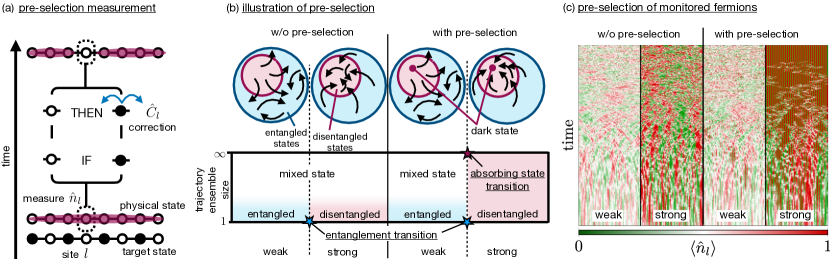
Figure 1: Pre-selection concept: (a) Illustration in a fermion hopping model with local monitoring. The outcome of measurements of $\hat{n}_{l}$ are recorded, and action is taken conditioned on its compatibility with a fixed target state by an IF-THEN clause discussed in the main text. Here a Néel state is targeted. If the occupation matches the one of this state, no feedback is applied. If the correlation is incompatible with the Néel state, a unitary hopping process is imposed. (b) General mechanism. Wave functions undergoing Hamiltonian dynamics subject to local measurements display two different dynamical phases: for weak (rare) measurements, the Hamiltonian scrambles information and each initial wave function evolves into a (sub-) extensively entangled state. For strong (frequent) measurements, each wave function enters a quantum Zeno regime and obeys area law entanglement. Despite their different entanglement structure, the wave functions in both phases are subject to randomness in space and time, and their ensemble always approaches a maximally mixed state. In the presence of pre-selection, a unique dark state is introduced. The presence of the dark state does not affect the dynamics in the weak measurement phase, but due to feedback, it acts as an attractor of disentangled wave functions in the quantum Zeno regime. Each disentangled wave function evolves towards the dark state, making the ensemble a pure, disentangled state. (c) Unconditioned vs. pre-selected evolution for monitored free fermions. Pre-selection successfully distinguishes the weak and the strong measurement phase: for weak measurements each fermion wave function obeys a logarithmic entanglement growth and a random density distribution. For strong measurements, each state evolves into a Néel state with alternating particle number distribution. Without pre-selection, both weak and strong measurements yield a random state, which can only be characterized by its entanglement entropy.

Pre-selection – The goal is to pull the MIPT to the observable level by modifying the dynamics such that it uncovers a phase transition in the density matrix $\hat{\rho}$, averaged over the measurement outcomes. In general, the averaged update of a state in a time step $\delta t$ can be written as a dynamical Kraus map

$$\hat{\rho}_{t+\delta t}=\hat{\mathcal{X}}[\hat{\rho}_{t}]\delta t,$$ (1)

with a time-local, completely positive, and trace preserving generator $\hat{\mathcal{X}}$. We denote the generator for the unmodified averaged unitary and measurement dynamics by $\hat{\mathcal{X}}^{(0)}$. Generically, the evolution has only one stable dynamical fixed point, namely, the maximally mixed state $\hat{\rho}\propto\hat{\mathds{1}}$, which obeys $\hat{\mathcal{X}}^{(0)}[\hat{\mathds{1}}]=0$. This is readily verified in the temporal continuum limit $\delta t\to 0$, where the generator takes Lindblad form,

$$\hat{\mathcal{X}}[\hat{\rho}]=-i[\hat{H},\hat{\rho}]+\sum_{l}\hat{L}_{l}\hat{\rho}\hat{L}_{l}^{\dagger}-\tfrac{1}{2}\{\hat{L}_{l}^{\dagger}\hat{L}_{l},\hat{\rho}\},$$ (2)

with $l$ labelling lattice sites. We consider measurements of local operators $\hat{L}_{l}^{(0)}$ with eigenvalues $\{\lambda_{1},\lambda_{2}\}$ spanning a two-dimensional Hilbert space. This yields the unmodified Hermitian Lindblad operators

$$\hat{L}_{l}^{(0)}=(\hat{L}_{l}^{(0)})^{\dagger}=\lambda_{1}\hat{P}_{l}+\lambda_{2}(\hat{\mathds{1}}-\hat{P}_{l}),\text{ with }\hat{P}_{l}=|{\lambda_{1}}\rangle\langle{\lambda_{1}}|,$$ (3)

with $\hat{P}_{l}^{2}=\hat{P}_{l}$. Examples are measurements of the spin orientation $\hat{Z}_{l}\,\,(\lambda_{1,2}=\pm 1)$ with $\hat{P}_{l}=(\hat{\mathds{1}}-\hat{Z}_{l})/2$ or fermion particle number $\hat{n}_{l}\,\,(\lambda_{1,2}=0,1)$ with $\hat{P}_{l}=\hat{\mathds{1}}-\hat{n}_{l}$.

In order to make the transition observable, we will introduce modifications of the generator $\hat{\mathcal{X}}^{(0)}\to\hat{\mathcal{X}}$ ($\hat{H}^{(0)},\hat{L}^{(0)}\rightarrow\hat{H},\hat{L}$) such that the following three conditions are obeyed:
(c1) There exists a dark state $\hat{\rho}_{D}=|D\rangle\langle D|$ of the full generator, i.e., $\hat{\mathcal{X}}[\hat{\rho}_{D}]=0$, which represents one possible measurement outcome.
(c2) The dark state is the unique stationary solution.
(c3) All modifications preserve the symmetries of the original problem and are irrelevant in the renormalization group (RG) sense.

Condition (c1) pre-selects a representative state of the measurement outcomes, and it can be equipped with an extensive order parameter, which eases experimental detection in many-body systems. Without loss of generality, we associate the projectors $\hat{P}_{l}$ with the ‘right’ measurement outcome, which is compatible with the dark state $\hat{P}_{l}\hat{\rho}_{D}=\hat{\rho}_{D}$. For local measurements, $\hat{\rho}_{D}$ is a product state. (c2) introduces a directionality in the evolution in Hilbert space: iterating the dynamical map ultimately filters out the state $\hat{\rho}_{D}$. In particular, the maximally mixed state ceases to be a dynamical fixed point of the averaged evolution. (c3) ensures that the modified dynamics is consistent with the original transition, and its universality class remains unaltered.

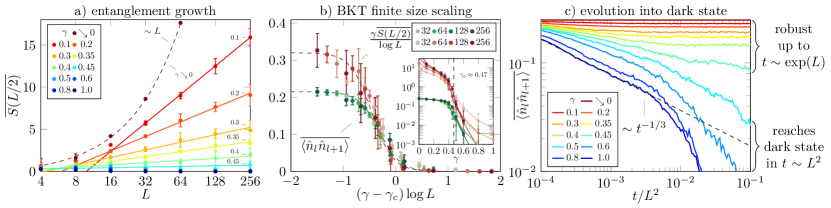
Figure 2: Absorbing state phase transition of monitored free fermions with pre-selection. (a) Growth of the half-chain entanglement entropy $S(L/2)$ with system size $L$. In the weak measurement phase ($\gamma\lesssim 0.47$), the entanglement grows logarithmically $S(L/2)\sim\tfrac{c_{\text{eff}}}{3}\log L$, and it vanishes in the strong measurement phase ($c_{\text{eff}}=0$) since the entanglement entropy in the Néel state is exactly zero (data points for $\gamma>0.47$ overlap). In the limit of vanishing measurement strength, a volume-law growth of the entanglement is observed. (b) Finite size scaling of the entanglement entropy and the ensemble averaged density-density correlation function $\langle\hat{n}_{l}\hat{n}_{l+1}$, extracted after an evolution time of $t=0.1L^{2}$. The scaling collapse reveals that both the entanglement entropy and the ensemble order parameter indicate a phase transition at the same critical measurement strength $\gamma_{c}=0.47$. Here, the exact vanishing of $S(L/2)$ and $\langle\hat{n}_{l}\hat{n}_{l+1}\rangle$ for $\gamma>0.47$ reduces the uncertainty in determining $\gamma_{c}$ compared to the unmodified MIPT, which was reported at a comparable value of $\gamma_{c}=0.31$ Alberton et al. (2021). The data displays BKT essential scaling with an exponential divergence of the correlation length $\log\xi\sim|\gamma-\gamma_{c}|^{-1}$. This demonstrates the connection of the absorbing state phase transition in the ensemble average and the entanglement transition on the level of individual trajectories. At the critical point and in the thermodynamic limit, both the order parameter and the entanglement entropy undergo a discontinuous jump from $\langle\hat{n}_{l}\hat{n}_{l+1}\rangle\approx 0.21$ or $c_{\text{eff}}\approx 2.0$ to zero. The inset shows the unrescaled data, with dashed lines as guides to the eye. (c) The evolution of the order parameter $\langle\hat{n}_{l}\hat{n}_{l+1}\rangle$ displays a characteristic behavior in both phases: in the strong measurement phase, the dark state is reached after an algebraic time scale $t\sim L^{2}$ resulting from the diffusive redistribution of number-conserved particles under strong measurements. The initial relaxation follows a power law decay $\sim t^{-1/3}$ of the order parameter. In the weak measurement phase, the order parameter saturates on a plateau, which is robust up to exponentially long time scales $t\sim\exp(L)$ in the system size. This phenomenology in the dynamics gives a further parallel to absorbing state transitions, and to purification transitions Gullans and Huse (2020a).

These three conditions can be implemented in various distinct ways. Their common thread is to condition the evolution at a given time step on the measurement outcome of the previous one, in the sense of an ‘IF-THEN’ clause: if a certain measurement outcome is obtained, then depending on the compatibility with the target state $\hat{\rho}_{D}$ the state update is selected. In particular, below we expose three principal strategies to implement this goal, which we dub ‘classical feedback’, ‘quantum feedback’ and ‘quantum simulation’.

The feedback strategies rely on reading out the measurement. In the classical version, the Hamiltonian $\hat{H}^{(0)}\to\hat{H}[\hat{\rho}]$ is chosen conditioned on the detected state $\hat{\rho}$ such that steering in Hilbert space is achieved, indeed akin to feedback Wiseman and Milburn (1993a); Wiseman (1994); Ivanov et al. (2020). The evolution then becomes non-linear in the state. The alternative quantum strategy builds on correcting ‘wrong’ measurement results immediately Roy et al. (2020); Santos et al. (2020): it modifies $\hat{L}^{(0)}\to\hat{L}$ by sending $(\hat{P},\hat{\mathds{1}}-\hat{P})\to(\hat{P},\hat{C}(\hat{\mathds{1}}-\hat{P}))$ with unitary correction $[\hat{C},\hat{P}]\neq 0$. The quantum simulation approach refrains entirely from surfacing the measurement outcomes $\hat{L}^{(0)}$ to the experimenter’s classical world: Instead, internal quantum action resulting from coupling to an environment is taken Diehl et al. (2008); Verstraete et al. (2009); Weimer et al. (2010), but here conditioned on the effect of the operator $\hat{L}^{(0)}$. This relaxes the constraints – measurements need not be read out and $\hat{C}$ need not be unitary – without modifying (c1)-(c3) or the phase transition on the average ensemble. In the quantum strategies, the evolution remains linear in the state, but the Lindblad operators $\hat{L}$ become non-Hermitian, implementing the desired directionality in Hilbert space. Thus they bear some similarities with the scenario of dark state cooling and associated phase transitions Diehl et al. (2010); Marino and Diehl (2016), with the key qualitative difference that these usually do not feature a dark state in the entire parameter space.

How can a phase transition then occur, if the dark state is a stationary solution globally in parameter space? An insight can be obtained from a parallel to absorbing state phase transitions, such as directed percolation Hinrichsen (2000); Ódor (2004). There as well, exists a global absorbing state. However, for generic initial conditions, it is only reached below a certain threshold, while it will be missed by the dynamics (for times sub-exponential in the system size) above it Hinrichsen (2000). This defines absorbing and active phases, respectively, and there is a critical point separating them. The transitions here can be manifestly in the quantum regime, witnessed, e.g., in a $1+1$ dimensional example below, reminiscent of a zero temperature quantum phase transition.

MIPT for monitored free fermions. – We illustrate each pre-selection scheme for a MIPT of monitored free fermions Alberton et al. (2021). The fermion Hamiltonian describes hopping on a half-filled chain of length $L$ (units are set by the Hamiltonian)

$$\hat{H}^{(0)}=\sum_{l}\hat{h}_{l}r_{l},$$ (4)

with $\hat{h}_{l}=\hat{c}^{\dagger}_{l}\hat{c}_{l+1}$+H.c. for fermions $\hat{c}^{\dagger}_{l},\hat{c}_{l}$, and $r_{l}=1$ is the coupling parameter here. The Hamiltonian competes with measurements, either weak-continuous or projective, of non-commuting observables $[\hat{L}_{l}^{(0)},\hat{h}_{l}]\neq 0$. Here, we measure the local densities $\hat{L}^{(0)}_{l}=\hat{n}_{l}=\hat{c}^{\dagger}_{l}\hat{c}_{l}$ with rate $\gamma$.

This competition drives a MIPT between two different entanglement phases Alberton et al. (2021); Buchhold et al. (2021): for small rates $\gamma$ (weak measurements), each wave function is scrambled and approaches a state with logarithmic entanglement growth, reminiscent of a conformally invariant, quantum critical state. For large $\gamma$ (strong measurements), a quantum Zeno regime emerges. It hosts area law entangled wave functions, close to instantaneous eigenstates of each $\hat{L}^{(0)}_{l}$. Both regimes are separated by a measurement-induced Berezhinskii-Kosterlitz-Thouless (BKT) phase transition Buchhold et al. (2021); Bao et al. (2021).

Classical pre-selection. – In order to lift the measurement-degeneracy, pre-selection is implemented by making $\hat{H}^{(0)}\to\hat{H}[\hat{\rho}]$ state-dependent via

$$r_{l}\rightarrow r_{l}[\hat{\rho}]\text{ but leaving}\ \hat{L}_{l}\equiv\hat{L}_{l}^{(0)}.$$ (5)

A suitable absorbing state with $[\hat{H}[\hat{\rho}_{D}],\hat{\rho}_{D}]=0$ is the Néel state $|D\rangle=|01010...\rangle$, populating either the even or the odd sites of the chain, see Fig. 1(d). A convenient choice for the state-dependence of $r_{l}[\hat{\rho}]$ is

$$r_{l}[\hat{\rho}]=2-(\lfloor\langle\hat{n}_{l-1}\rangle\rfloor-\lfloor\langle\hat{n}_{l}\rangle\rfloor)^{2}-(\lfloor\langle\hat{n}_{l+1}\rangle\rfloor-\lfloor\langle\hat{n}_{l+2}\rangle\rfloor)^{2},$$

where $\lfloor...\rfloor$ indicates rounding to the nearest integer. This conditions the couplings $r_{l}$ on the instantaneous expectation values $\langle\hat{L}_{l}^{(0)}\rangle$ of the measured operators. In an experiment, these can be obtained by simulating the instantaneous state $\hat{\rho}$ (e.g., for Gaussian systems or stabilizer states, see Appendix A) or be extracted from the measurement outcomes, e.g., by applying an appropriate noise filter Young et al. (2021).

An intuitive understanding obtains in the limiting cases: (i) For weak measurements, the operators $\hat{h}_{l}$ scramble the observables $\hat{n}_{l}$. The state becomes translation invariant $\langle\hat{n}_{l}\rangle=1/2$ and $r_{l}[\hat{\rho}]\rightarrow 1$ is effectively state-independent. (ii) For strong measurements, $\hat{\rho}$ enters a quantum Zeno regime, where $\langle\hat{n}_{l}\rangle\hat{\rho}\sim\hat{n}_{l}\hat{\rho}$. We can thus promote $r_{l}[\hat{\rho}]\rightarrow\hat{r}_{l}\equiv 2-(\hat{n}_{l-1}-\hat{n}_{l})^{2}-(\hat{n}_{l+1}-\hat{n}_{l+2})^{2}$ to an operator with $r_{l}[\hat{\rho}]\hat{\rho}=\hat{r}_{l}\hat{\rho}$. A directed evolution towards $\hat{\rho}_{D}$ is implemented when the product $\hat{h}_{l}\hat{r}_{l}$ is non-Hermitian, i.e., when $[\hat{h}_{l},\hat{r}_{l}]\neq 0$. Both limits, (i) and (ii), allow us to effectively eliminate the state dependence in $\hat{H}[\hat{\rho}]$, yielding two types of Hamiltonians $\hat{H}_{w,s}$: for weak measurements $\hat{H}_{w}\equiv\hat{H}^{(0)}$ and thus is unmodified by pre-selection. For strong measurements $\hat{H}_{s}\equiv\sum_{l}\hat{h}_{l}\hat{r}_{l}$ is non-Hermitian and implements an IF-THEN condition, steering towards $\hat{\rho}_{D}$.

Fig. 2 demonstrates the MIPT with pre-selection for a continuous-measurement scheme (see Appendix A): The entanglement scaling is inherited in the pre-selected case, but now accompanied by a phase transition for the order parameter $\sum_{l}\langle\hat{n}_{l}\hat{n}_{l+1}\rangle$. The critical behavior is governed by the essential scaling of a BKT transition. The transition can be probed experimentally by standard means, like a single-shot measurement of the density distribution.

Quantum pre-selection. – We modify the Hamiltonian in Eq. (4) such that the Néel state is again a dark state:

$$\hat{H}^{(0)} \rightarrow\hat{H}=\sum_{l\text{ odd}}\hat{n}_{l}(\hat{h}_{l+1}+\hat{h}_{l-2})+\sum_{l\text{ even}}(1-\hat{n}_{l})(\hat{h}_{l+1}+\hat{h}_{l-2}).$$

The directionality is implemented by an IF-THEN condition acting right after a ‘wrong’ (incompatible with target dark state) measurement result $\hat{n}_{l\,\text{odd}}\to 1$ has been obtained on odd sites. Wrong results can be corrected by applying a quasi-local unitary gate operation $\hat{C}_{l}$ with $[\hat{C}_{l},\hat{L}^{(0)}]\neq 0$. Here we take $\hat{C}_{l}=\exp(-i\tfrac{\pi}{2}\hat{h}_{l})$. This preserves the symmetries, and works both for projective measurements and quantum jump Daley (2014) evolution protocols (see Appendix B). The principle of the steering towards the dark state is this: If a ‘right’ measurement result has been recorded, the projector $\hat{P}_{l}$ evolves the state towards $\hat{\rho}_{D}$. If a ‘wrong’ measurement result has been recorded, the state is projected by $\hat{Q}_{l}=\hat{\mathds{1}}-\hat{P}_{l}$ away from $\hat{\rho}_{D}$. We then rotate it back onto the dark state by the unitary $\hat{C}_{l}$:

$$\text{`right'}:\hat{\rho}\rightarrow\hat{P}_{l}\hat{\rho}\hat{P}_{l}/\langle\hat{P}_{l}\rangle,\ \text{`wrong'}:\hat{\rho}\rightarrow\hat{C}_{l}\hat{Q}_{l}\hat{\rho}\hat{Q}_{l}\hat{C}_{l}^{\dagger}/\langle\hat{Q}_{l}\rangle.$$

The average ensemble of pre-selected wave functions then follows the Lindblad master equation (see Appendix B)

$$\partial_{t}\hat{\rho}=-i[\hat{H},\hat{\rho}]-\frac{\gamma}{2}\sum_{l}\{[\hat{n}_{l},[\hat{n}_{l},\hat{\rho}]]+\{\hat{L}_{l}^{\dagger}\hat{L}_{l},\hat{\rho}\}-2\hat{L}_{l}\hat{\rho}\hat{L}_{l}^{\dagger}\},$$ (6)

with Lindblad operators $\hat{L}_{l}$ on odd/even sites $l$

$$\text{ odd: }\hat{L}_{l}=\hat{C}_{l}\hat{L}^{(0)}_{l}=\hat{n}_{l}\hat{n}_{l+1}+i\hat{c}^{\dagger}_{l+1}\hat{c}_{l},\ \text{ even: }\hat{L}_{l}=\hat{L}^{(0)}_{l}=\hat{n}_{l}.$$

The master equation (6) turns the fermion MIPT in individual wave functions into an absorbing state transition for the ensemble: The repeated application of both $\hat{H}$ and $\hat{L}_{l\text{ odd}}$ pushes any initial state into the Néel state $\hat{\rho}_{D}$, which is the unique dark state. Active and inactive phases are distinguished by the characteristic time scale at which $\hat{\rho}_{D}$ is reached. For strong measurements ($\gamma\gg 1$), the state $\hat{\rho}$ is nearly diagonal in the fermion number basis and the modified Lindblad operators cause a diffusive motion towards the Néel state (reached on time scales $t\sim L^{2}$ with system size $L$). The absorbing property of the Néel state in this regime is confirmed by a mean-field analysis of the Lindbladian for a homogeneous system of infinite size (see Appendix C). It predicts that the Néel state is the only stationary state for $\gamma\geq 2$. For weak measurements $\gamma\ll 1$, however, the enhanced superposition of particles leads to a drastic enlargement of the accessible Hilbert space, and a slowing down of the relaxation towards the Néel state. It can only be reached on time scales growing with the size of the Hilbert space $t\sim\exp(L)$. In the mean-field equations, this is revealed by the emergence of a second stationary solution: an active state with $\langle\hat{n}_{l\text{ odd}}\rangle=\langle 1-\hat{n}_{l\text{ even}}\rangle=\tfrac{4-\gamma^{2}}{8}$ for $\gamma<2$. While the Néel state remains stationary, any other initial configuration approaches the active state, whose lifetime diverges in the $L\to\infty$ limit. This confirms the phenomenology of an absorbing state phase transition. In order to examine the long-wavelength dynamics beyond mean-field, we work in the spatial continuum limit, which for number-conserving fermion dynamics amounts to the bosonization framework Buchhold et al. (2021). In bosonization, the irrelevance of the modifications leads to $\hat{H}\approx\hat{H}^{(0)}$ and $\hat{L}_{l}\approx\hat{L}_{l}^{(0)}$ up to (globally crucial) gradient terms. Quantitatively, the dynamics is described by a non-Hermitian Sine-Gordon theory, which predicts the absorbing state transition to be BKT. This complements analytically our numerical results for the classical scheme (Fig. 2). In particular, the term describing the noise level in the effective theory is RG irrelevant, reflecting the existence of a dark state and preserving the scaling behavior characteristic of a $1+1$ dimensional quantum BKT scenario (see Appendix D).

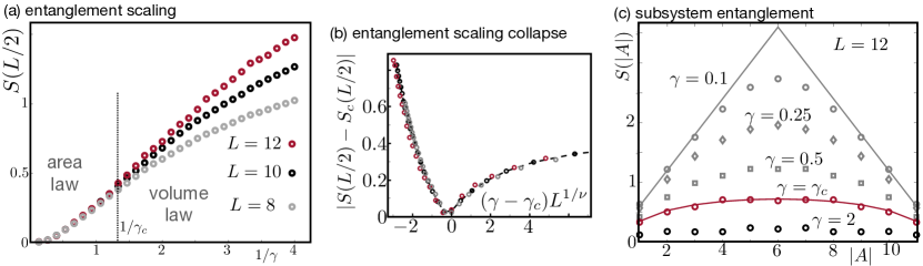
Figure 3: Measurement-induced phase transition in a Rydberg array. We numerically simulate the time evolution of an array of $L$ qubits, generated by the Rydberg Hamiltonian in Eq. (7) and projective measurements of the orientation $\hat{Z}_{l}$ of each qubit. Changing the rate $\gamma$ at which measurements are performed, the system undergoes an entanglement phase transition in the stationary state. It is witnessed in the von Neumann entanglement entropy $S(|A|)=-\text{tr}(\hat{\rho}_{A}\ln\hat{\rho}_{A})$, where $\hat{\rho}_{A}=\text{tr}_{\bar{A}}|\psi\rangle\langle\psi|$ is the density matrix of a contiguous subsystem $A$ after tracing out its complement $\bar{A}$. (a) For small measurement rates (weak measurements), the entanglement entropy for different system sizes obeys a volume law $S(L/2)\sim L$. For large measurement rates (strong measurements) instead, it collapses onto an area law $S(L/2)\sim\text{const.}$ Both regimes are separated by a critical point at $\gamma_{c}\approx 0.77$. (b) Finite size scaling of the entanglement entropy is consistent with a correlation length critical exponent $\nu=\tfrac{4}{3}$ for bond percolation, similar to what has been found in Ref. Zabalo et al. (2020) for a related MIPT in Haar- and Clifford random circuits. (c) The entanglement entropy for a total system size $L=12$ and different subsystem sizes $|A|$ reveals the MIPT from volume- to area law. For weak measurements at $\gamma=0.1$, it displays a volume law with a nearly perfect linear growth $S(|A|)\approx 0.6\min\{|A|,L-|A|\}$, (grey solid line). At the critical value $\gamma=\gamma_{c}$, it is well described by a logarithmic function $S(|A|)=0.56\ln(\sin(\pi|A|/L))+s_{0}$ as in conformal field theory. For strong measurements ($\gamma=2$) it approaches a constant which is independent of $|A|$.

Quantum simulation. – An even simpler practical route to extract the quantitative properties of the MITP is when an engineered environment Diehl et al. (2008); Verstraete et al. (2009); Barreiro et al. (2011) implements the IF-THEN condition autonomously without the need of measurement readout. Indeed, the master equation (6) reveals a general equivalence between MIPTs with pre-selection and absorbing state phase transitions in open systems: whenever the Lindblad operators $\hat{L}_{l}$ can be written as a projector $\hat{\mathds{1}}-\hat{P}_{l}$ (IF) followed by an operator imposing directionality $\hat{C}_{l}$ with $[\hat{C}_{l},\hat{L}_{l}]\neq 0$ (THEN), the corresponding absorbing phase transition has a MIPT counterpart in monitored systems. When the operator $\hat{C}_{l}$ is imposed by the coupling to an environment, its unitarity can be dropped, yielding more flexibility for implementing MIPTs with open systems. In particular, one might choose $\hat{C}^{(\pm)}_{l\,\text{odd}}=\hat{h}_{l\pm 1}$, $\hat{C}_{l\,\text{even}}=\hat{\mathds{1}}$, i.e., $\hat{L}^{(\pm)}_{l\,\text{ odd}}=\hat{c}^{\dagger}_{l\pm 1}\hat{c}_{l}$. In the continuum limit, these operators become $\pm(\partial_{x}\hat{c}^{\dagger}_{x})\hat{c}_{x}+\hat{n}_{x}$. The gradient terms lift the degeneracy of the dephasing operators $\hat{n}_{l}$ and, together with the Hamiltonian $\hat{H}$, provide a unique dark state. However, they do not modify universal properties due to their RG irrelevance.

MIPT and pre-selection in Rydberg arrays. – As a second realization of a pre-selected MIPT, we discuss an array of Rydberg atoms in the facilitation regime Gutiérrez et al. (2017); Helmrich et al. (2018); Festa et al. (2022). Each atom $l$ hosts a qubit described by Pauli operators $\hat{X}_{l},\hat{Y}_{l},\hat{Z}_{l}$. The dynamics of $L$ qubits is generated by the Hamiltonian Marcuzzi et al. (2016); Lesanovsky and Garrahan (2013)

$$\hat{H}=\sum_{l}\hat{n}_{l}(\hat{X}_{l-1}+\hat{X}_{l+1}),\text{ with }\hat{n}_{l}\equiv\tfrac{1}{2}(\hat{\mathds{1}}+\hat{Z}_{l}).$$ (7)

At each time step $dt$, it acts like a controlled-$\exp(-idt\hat{X})$ gate on neighboring qubits. This yields the dark state $|D\rangle=|00...00\rangle$, while any other state in the computational basis quickly approaches a volume law entangled state. A MIPT is ensured when the entanglement growth caused by the Hamiltonian is put into competition with disentangling measurements of the qubit orientation $\hat{Z}_{l}$, with scaling exponents consistent with two-dimensional bond percolation Bao et al. (2020); Zabalo et al. (2020), see Fig. 3.

In fact, a pre-selection quantum simulation scheme for this model has already been implemented in experiment (yet violating criterion (c3)) Gutiérrez et al. (2017); Helmrich et al. (2018); Festa et al. (2022): Consider projective measurements of $\hat{Z}_{l}$, as shown in Fig. 3. The Hamiltonian possesses no particular symmetry, thus a natural choice to implement pre-selection is

$$\hat{C}_{l}=\hat{X}_{l}\to\hat{L}_{l}=|0\rangle\langle 1|_{l}\equiv\hat{\sigma}^{-}_{l}.$$ (8)

While this operators steers towards $|D\rangle=|00...00\rangle$ as unique dark state, the local operator $\hat{X}_{l}$ represents a relevant perturbation and is expected to change the universal behavior. Physically, $\hat{L}_{l}$ describes spontaneous emission. Indeed, facilitated Rydberg arrays subject to decay are suspected to undergo an absorbing state phase transition in the directed percolation universality class Marcuzzi et al. (2016); Gutiérrez et al. (2017). In order to make the correction RG irrelevant, meeting (c3), we propose the conditioned version

$$\hat{C}_{l,\pm}=(\hat{\mathds{1}}-\hat{n}_{l\pm 1})\hat{X}_{l}\to\hat{L}^{\pm}_{l}=\hat{\sigma}_{l}^{-}(\hat{n}_{l}-\hat{n}_{l\pm 1})=\pm(\nabla\hat{\sigma}_{l}^{-})\hat{n}_{l}.$$ (9)

While $\hat{C}_{l}$ is not unitary, implementation of $\hat{L}_{l}$ in controlled quantum platforms Weimer et al. (2010); Barreiro et al. (2011); Chertkov et al. (2022) seems in reach for the quantum simulation of a MIPT.

Conclusion. – Pre-selection reveals the physical meaning of MIPTs in terms of quantum absorbing state phase transitions in representative wave functions. This result is rationalized by the individual measurement trajectories hosting the same information as the entire ensemble in a large system. In this sense, it parallels post-selection, but it avoids exponential overhead. On the practical side, this opens up a clear path towards experimental observability of MIPTs in controlled quantum platforms. On the theory side, it sparks characterizing novel non-equilibrium universality classes in the quantum regime. While we demonstrated the tight connection of stationary behaviors of MITPs and pre-selected scenarios, a particular challenge is posed by exploring their mutual relation in terms of dynamics.

Note added: During completion of this manuscript we became aware of related work, discussing an example of a MIPT made observable by feedback Iadecola et al. (2022).

Appendix A Classical pre-selection for continuously monitored fermions

Here, we provide the theoretical background for pre-selected monitored fermion dynamics in the classical feedback variant, cf. Fig. 2. In order to continuously monitor a set of observables $\{\hat{L}_{l}^{(0)}\}$ with a rate $\gamma$, they are weakly coupled to an auxiliary system Szyniszewski et al. (2019); Wiseman and Milburn (1993b); Yang et al. (2018), which is then frequently measured Jacobs and Steck (2006), i.e., on time scales much faster than the typical evolution time of the system. This reveals the so-called currents $J_{l,t}=\langle\hat{L}_{l}^{(0)}\rangle_{t}+\tfrac{dW_{l}}{2\gamma dt}$, where $\langle\hat{L}_{l}^{(0)}\rangle_{t}=\Tr(\hat{L}_{l}^{(0)}\hat{\rho}_{t}^{c})$ is the instantaneous expectation value, and $dt$ the typical time between successive measurements. Here $\hat{\rho}_{t}^{c}=|\psi\rangle\langle\psi|$ is the so-called conditioned state, i.e., the wave function conditioned on all previous measurement outcomes. The randomness of the measurement outcome is encoded in the Wiener increment $dW_{l}$ with variance $\gamma dt$. In the absence of environmental dissipation, the quantum system remains in a pure state wave function $\ket{\psi}$, which is conditioned on the stream of currents $\{J_{l,t}\}$. The temporal update of the conditioned state is

$$\partial_{t}\hat{\rho}_{t}^{c}= i[\hat{\rho}_{t}^{c},\hat{H}]-\tfrac{\gamma}{2}\sum_{l}[\hat{L}_{l}^{(0)},[\hat{L}_{l}^{(0)},\hat{\rho}_{t}^{c}]]$$ (10)

$$+2\gamma\sum_{l}(J_{l,t}-\langle\hat{L}_{l}^{(0)}\rangle_{t})\{\hat{L}_{l}^{(0)}-\langle\hat{L}_{l}^{(0)}\rangle_{t},\hat{\rho}_{t}^{c}\}.$$

When the currents at each time step are known from the measurement read-out, the state update is deterministic. It can, e.g., be simulated in real time parallel to the experiment for systems of low complexity, such as small systems or systems described by Gaussian wave functions. The latter thus provides a case when the instantaneous expectation values $\langle\hat{L}^{(0)}_{l}\rangle$ can be extracted in every time step from simulation. We use this insight in the classical pre-selection scheme for monitored free fermions that is discussed in the main text and Fig. 2, considering a state-dependent Hamiltonian $\hat{H}=\hat{H}[\hat{\rho}^{c}]=\hat{H}[\{\langle\hat{L}^{(0)}_{l}\rangle\}]$.

An alternative scheme, e.g., applicable for more complex wave functions that cannot be simulated in real-time, may estimate the instantaneous expectation values directly from the measurement outcomes, i.e., the currents $J_{l,t}$, by applying appropriate filtering, such as using a Kalman Wieczorek et al. (2015) or a low pass filter Young et al. (2021). Advanced filtering schemes thus can represent an alternative way to resolve MIPTs in the classical feedback scheme. A further alternative is represented by the quantum feedback and quantum simulation variants discussed in the main text, which do not require the classical inputs.

In order to simulate the free fermion setup as described in the main text in practice, we parameterize the conditioned state as $\hat{\rho}^{c}=\ket{\psi}\bra{\psi}$ with $\ket{\psi}_{t}=\prod_{l=1}^{L/2}\left(\sum_{j=1}^{L}U_{j,l}(t)\hat{c}_{j}^{\dagger}\right)\ket{0}$ (cf. Cao et al. (2019); Alberton et al. (2021)), and the $L\times L/2$ matrix $U$ contains normalized single-fermion wave functions. Up to leading order $\mathcal{O}(dt)$, the evolution of $U$ is computed by matrix multiplication

$$U(t+dt)= \text{diag}(e^{dW_{1,t}+\gamma dt(2\langle\hat{n}_{1}\rangle_{t}-1)},\dots,e^{dW_{L,t}+\gamma dt(2\langle\hat{n}_{L}\rangle_{t}-1)})$$ (11)

$$\times e^{-ih[U(t)]dt}U(t).$$

Here, we indicate that with pre-selection, the Hamiltonian matrix $h[U(t)]$ is itself a function of the state, i.e., the time-dependent matrix $U(t)$, with $\langle\hat{n}_{l}\rangle_{t}=[U(t)U(t)^{\dagger}]_{l,l}$. It is a hopping matrix with entries $h_{l,l+1}[U(t)]=h_{l+1,l}[U(t)]=2-(\lfloor\langle\hat{n}_{l-1}\rangle\rfloor-\lfloor\langle\hat{n}_{l}\rangle\rfloor)^{2}-(\lfloor\langle\hat{n}_{l+1}\rangle\rfloor-\lfloor\langle\hat{n}_{l+2}\rangle\rfloor)^{2}=r_{l}[\hat{\rho}_{t}^{c}]$ and zero otherwise. This implements the classical pre-selection routine described in the main text. After each time step, for which we choose $dt=0.05$, normalization is implemented by performing a QR-decomposition $U=QR$ and setting $U=Q$.

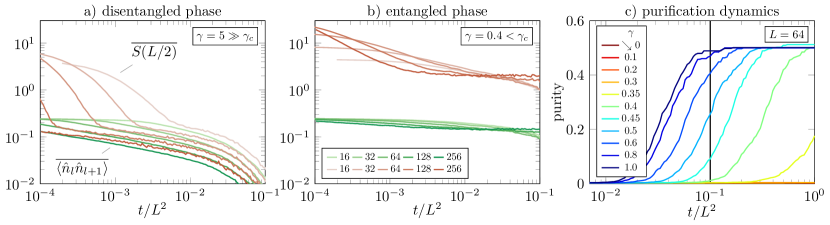
Figure 4: (a), (b) System-size dependence of the approach to the target state. For strong measurements $\gamma\gg\gamma_{c}$, the feedback pushes the system into the target state starting at $t\approx L^{2}/100$, independently of the precise value of $\gamma$ and for a wide range of $L$. At the same timescale, weak measurements $\gamma<\gamma_{c}$ lead to a plateau for the proximity to the target state and the entanglement entropy. For sufficiently large system sizes $L$, we observe no decay plateau of the plateau on algebraic time scales, which confirms our expectation of an exponentially long lifetime $t\sim\exp(L)$ of the active state. This means that we observe stationary behavior in both regimes at $t\approx L^{2}/10$ and we pick this timescale to study the stationary state properties in both regimes. For $\gamma\approx\gamma_{c}$, large $L$ are needed to clearly identify one of the two cases, which we treat by finite size scaling analysis at $t=L^{2}/10$. Before the stationary state is established, we observe a characteristic algebraic scaling regime, $\overline{\langle\hat{n}_{l}\hat{{n}}_{l+1}\rangle}\sim t^{-\sigma}$ with $\sigma\approx 1/3$ in the strongly measured regime. (c) For strong measurements the trajectory ensemble purifies at the same timescale, while weak measurements leave it fully mixed for exponentially long times. The final purity is $1/2$ due to the degeneracy of the target state.

Each trajectory is initialized in a random, half filled product state (e.g. $\ket{01101001\dots}$), which is evolved under an unconditioned Hamiltonian ($r_{l}=1$) for a short period ($t=-5$ to $t=0$) to reach an entangled intial wave function at $t=0$. Then, the classical pre-selection scheme is applied as described above. During the evolution, we compute the entanglement entropy $S(L/2)=-\Tr\hat{\rho}^{c}_{L/2}\log\hat{\rho}^{c}_{L/2}$ for the half-system reduced density matrix $\hat{\rho}^{c}_{L/2}=\Tr_{L/2}\hat{\rho}^{c}$, the order parameter $\langle\hat{n}_{l}\hat{n}_{l+1}\rangle=\Tr\hat{n}_{l}\hat{n}_{l+1}\hat{\rho}^{c}\geq 0$ and the ensemble purity (see below). Each observable reaches a (quasi-) stationary plateau at times $t\sim\mathcal{O}(L^{2})$, as we show in Fig. 4. The algebraic scaling with system size results from the diffusive motion of particles in number-conserving systems subject to decoherence. It has to be distinguished from the exponentially long, asymptotic time-scale $t\sim\exp(L)$, growing with the size of the Hilbert space, on which the system always falls into the absorbing state, see Fig. 4. Throughout this work, we set the stationary values to be reached at $t=0.1L^{2}$, which turns out to yield consistent and converged expectation values, shown in Fig. 2. The observables at this timescale are extracted by averaging over many different trajectories (denoted by an overbar). Each result is then also time-averaged over the period $t=\frac{5}{6}L^{2}/10$ to $t=\frac{6}{5}L^{2}/10$ and fitted by linear regression, yielding the error estimates shown in Fig. 2.

Appendix B Quantum pre-selection for projective measurements and quantum jumps

Here, we derive the quantum master equation for pre-selection, Eq. (6) in the main text. We consider two cases, projective measurements and a quantum jump evolution, which yield analogous results. The master equation is conveniently derived from a continuous evolution equation of the wave function, the stochastic Schrödinger equation (SSE) Jacobs and Steck (2006); Alberton et al. (2021). For each trajectory, we make use of the conditioned state $\hat{\rho}^{c}=|\psi\rangle\langle\psi|$, i.e., the pure state wave function conditioned on all measurement outcomes. For a set of local measurements $\hat{L}_{l}^{(0)}$ denoted by an index $l$, e.g., spin orientation $\hat{L}_{l}^{(0)}=\hat{Z}_{l}$ or fermion density $\hat{L}_{l}^{(0)}=\hat{n}_{l}$, we introduce the projector $\hat{P}_{l}$ on one measurement outcome, e.g., $\hat{P}_{l}=(\hat{\mathds{1}}+\hat{Z}_{l})/2$ for spins and $\hat{P}_{l}=\hat{n}_{l}$ for fermions. We refer to the orthogonal projection as $\hat{Q}_{l}=\hat{\mathds{1}}-\hat{P}_{l}$. Without loss of generality, we assume that $\hat{P}_{l}$ is compatible with the dark state, such that $\hat{P}_{l}\hat{\rho}_{D}=\hat{\rho}_{D}$ and $\hat{Q}_{l}\hat{\rho}_{D}=0$. At each time step $dt$, the conditioned state evolves according to $\rho^{c}_{t+dt}=\rho^{c}_{t}+d\rho^{c}_{t}$ with

$$d\hat{\rho}^{c}_{t}= idt[\hat{\rho}^{c}_{t},\hat{H}]+\sum_{l}dW_{l}\left(p_{l}\frac{\hat{P}_{l}\hat{\rho}^{c}_{t}\hat{P}_{l}}{\langle\hat{P}_{l}\rangle_{t}}+(1-p_{l})\frac{\hat{Q}_{l}\hat{\rho}^{c}_{t}\hat{Q}_{l}}{\langle\hat{Q}_{l}\rangle_{t}}-\hat{\rho}^{c}_{t}\right).$$ (12)

Whether or not a measurement at coordinate $l$ is performed at this time step is determined by the discrete, random increment $dW_{l}=0,1$. It has expectation value $\mathds{E}(dW)=\gamma dt$, reflecting an average measurement rate $\gamma$. Once a measurement is performed, the Born probabilities are implemented by the random number $p_{l}=0,1$. It selects the measurement outcome associated with $\hat{P}_{l}$ with probability $\mathds{E}(p_{l})=\langle\hat{P}_{l}\rangle$. The statistical average of Eq. (12) yields the master equation

$$\partial_{t}\hat{\rho}=i[\hat{\rho},\hat{H}]-\gamma\sum_{l}[\hat{P}_{l},[\hat{P}_{l},\hat{\rho}]]$$ (13)

for the wave function ensemble $\hat{\rho}$. Due to the double commutator, the projector $\hat{P}_{l}$ can be replaced by the observable $\hat{L}_{l}^{(0)}$ and an appropriate numerical prefactor, e.g. $\hat{P}_{l}\to\hat{n}_{l}$ for fermions and $\hat{P}_{l}\to\tfrac{1}{2}\hat{Z}_{l}$ for spins.

With quantum pre-selection, we immediately correct each ‘wrong’ measurement result with a unitary $\hat{C}_{l}\hat{C}_{l}^{\dagger}=\hat{\mathds{1}}$. This replaces $\hat{Q}_{l}\hat{\rho}^{c}\hat{Q}_{l}\to\hat{C}_{l}\hat{Q}_{l}\hat{\rho}^{c}\hat{Q}_{l}\hat{C}_{l}^{\dagger}$ in Eq. (12) as outlined in the main text. This correction is state-independent and averaging Eq. (12) with correction yields

$$\partial_{t}\hat{\rho}=i[\hat{\rho},\hat{H}]-\frac{\gamma}{2}\sum_{l}\left([\hat{P}_{l},[\hat{P}_{l},\hat{\rho}]]+\{\hat{L}_{l}^{\dagger}\hat{L}_{l},\hat{\rho}\}-2\hat{L}_{l}\hat{\rho}\hat{L}_{l}^{\dagger}\right).$$

Here, the modified Lindblad operators $\hat{L}_{l}=\hat{C}_{l}\hat{Q}_{l}$ are non-Hermitian. They implement the IF-THEN condition: if the state $\hat{\rho}$ is locally in the target dark state, then $\hat{Q}_{l}\hat{\rho}=0$ and consequently $\hat{L}_{l}\hat{\rho}=0$. If, however, $\hat{Q}_{l}\hat{\rho}\neq 0$, then $\hat{C}_{l}$ rotates the state locally towards the dark state. We remark that the correction acts on each ‘wrong’ measurement outcome and therefore in the master equation above, the rate $\gamma$ at which the Lindblad operators act is locked onto the measurement rate. This is in principle different for the quantum simulation scheme, where an individual rate for both processes might be set by the bath degrees of freedom.

An analogous scheme can be implemented for a quantum jump evolution protocol Daley (2014). Here, each degree of freedom $l$ is coupled to a detector, which measures only one possible outcome of the observable. An example is the detection of a particle by light scattering: once a scattered photon is observed (the detector ‘clicks’), it indicates the presence of a particle. However, not observing a scattered photon does not rule out the presence of the particle. The pre-selection scheme works by performing an immediate correction after a wrong measurement outcome has been recorded, which in the quantum jump evolution can only be a ‘click’. In order to make contact to projective measurements above, we associat a ‘click’ with the projector $\hat{Q}_{l}$. When the detector ‘clicks’, which happens with a probability $\gamma dt\langle Q_{l}\rangle$, the state is projected by $\hat{Q}_{l}$. In the quantum jump protocol, the conditioned state follows the SSE

$$d\hat{\rho}^{c}= idt[\hat{\rho}^{c},\hat{H}]+\sum_{l}\left[d\tilde{W}_{l}\left(\frac{\hat{Q}_{l}\hat{\rho}^{c}\hat{Q}_{l}}{\langle\hat{Q}_{l}\rangle}-\hat{\rho}^{c}\right)-\frac{\gamma dt}{2}\{\hat{Q}_{l}-\langle\hat{Q}_{l}\rangle,\hat{\rho}^{c}\}\right].$$

Whether or not a ‘click’ is recorded is determined by the discrete stochastic increment $d\tilde{W}_{l}=0,1$, which clicks with probability $\mathds{E}(d\tilde{W}_{l})=\gamma dt\langle\hat{Q}_{l}\rangle$. Performing the statistical average over all measurement outcomes without pre-selection yields the master equation (13) with $\gamma\to\gamma/2$.

Pre-selection in the quantum jump evolution is implemented by modifying the projection of the state $\hat{Q}_{l}\hat{\rho}^{c}\hat{Q}_{l}\to\hat{C}_{l}\hat{Q}_{l}\hat{\rho}^{c}\hat{Q}_{l}\hat{C}_{l}^{\dagger}$ whenever a ‘click’ has been recorded. This yields the master equation for the ensemble average

$$\partial_{t}\hat{\rho}=i[\hat{\rho},\hat{H}]-\frac{\gamma}{2}\sum_{l}\left[\{\hat{L}_{l}^{\dagger}\hat{L}_{l}^{\phantom{\dagger}},\hat{\rho}\}-2\hat{L}_{l}^{\phantom{\dagger}}\hat{\rho}\hat{L}_{l}^{\dagger}\right].$$ (14)

It has the same rate and Lindblad operators as the ensemble evolution under projective measurements, but it does not feature the additional dephasing $\sim[\hat{P}_{l},[\hat{P}_{l},\hat{\rho}]]$.

Appendix C Mean-field treatment of fermions with quantum pre-selection

A more intuitive picture of the dynamics of fermions in the quantum feedback and the quantum simulation scheme is obtained when mapping the Néel state to a vacuum state $|01010..\rangle\to|00000..\rangle$ by performing an exact particle-hole transformation $\hat{c}_{l}\leftrightarrow\hat{c}_{l}^{\dagger}$ on every even site $l$. This maps the conditioned Hamiltonian in the main text to

$$\hat{H}\to\hat{H}_{\text{ph}}=\sum_{l}\hat{n}_{l}(\hat{h}_{l+1}+\hat{h}_{l-2})$$ (15)

with $\hat{h}_{l}=(\hat{c}_{l}\hat{c}_{l+1}+\text{H.c.})$. The Hermitian Lindblad operators are unchanged under this transformation since double commutators with $\hat{n}_{l}$ or $1-\hat{n}_{l}$ are identical. The non-Hermitian Lindblad operators on odd sites transform to $\hat{L}_{l}=\hat{n}_{l}(1-\hat{n}_{l+1})+i\hat{c}_{l}\hat{c}_{l+1}$, yielding the master equation

$$\partial_{t}\hat{\rho} =i[\hat{\rho},\hat{H}_{\text{ph}}]-\gamma\sum_{l\text{ even}}[\hat{n}_{l},[\hat{n}_{l},\hat{\rho}]]$$

$$-\frac{\gamma}{2}\sum_{l\text{ odd}}[\hat{n}_{l},[\hat{n}_{l},\hat{\rho}]]+\{\hat{n}_{l},\hat{\rho}\}-L_{l}\hat{\rho}\hat{L}_{l}^{\dagger}.$$ (16)

The Lindblad operators $\hat{n}_{l}$ compete with the coherent generation of particle and hole pairs in the Hamiltonian. The operators $\hat{L}_{l}$ guide the state towards the vacuum, once the Hamiltonian is sufficiently suppressed. The dark state is a translational invariant product state. Thus all correlation functions factorize according to Wick’s theorem. Close to the dark state, we can thus apply a mean-field theory, which captures the state-evolution in terms of the homogeneous density $n\equiv\langle\hat{n}_{l}\rangle$ and the pair-correlation $K\equiv i\langle c_{l}c_{l+1}-\text{H.c.}\rangle$. The mean-field theory becomes exact once the dark state is reached and represents a reasonable approximation in its vicinity. It yields

$$\partial_{t}n=n(4K-\gamma n),\ \partial_{t}K=4n(1-2n)-4\gamma K.$$ (17)

Inserting the stationary solution for the pair-correlation function $K=n(1-2n)/\gamma$ provides an evolution equation for the density alone

$$\partial_{t}n=\frac{n^{2}}{\gamma}(4-8n-\gamma^{2})$$ (18)

It shows that $n=0$, i.e., the absorbing state, is always a stationary solution of the time evolution. Furthermore, the absorbing state is the only stationary solution for $\gamma\geq 2$, making it a robust dark state in this regime. For $\gamma<2$, however, any non-zero initial density $n>0$ will lead to an algebraic growth of $n$ towards the value $n=\tfrac{1}{2}-\tfrac{\gamma^{2}}{8}$. This indicates a robust active phase with $n>0$ in this parameter regime. In summary, the mean-field analysis predicts both a robust active and a robust absorbing phase, separated by a critical point at $\gamma=\gamma_{c}=2$.

Appendix D Field theory for fermions with pre-selection

For $U(1)$-symmetric fermions in one dimension, mean-field theory provides only a very rough understanding of the critical dynamics at a quantum phase transition. An improved description is obtained from a long-wavelength theory, where the critical point is approached from the weak measurement phase. In this regime, the one-dimensional fermions are gapless and therefore described more accurately in terms of a hydrodynamic approach, namely via bosonization. Here, we work in the original basis (not particle-hole transformed). The fermion density and current in the spatial continuum $l\to x$ are described by boson field operators $[\partial_{x}\hat{\theta}_{x},\hat{\phi}_{x^{\prime}}]=i\delta(x-x^{\prime})$. In order to develop the effective long-wavelength description of the absorbing state phase transition of monitored fermions with pre-selection, we discuss the modifications to the Hamiltonian and the Lindblad operators in the bosonization framework.

In the fermionic description, the Lindblad operators $\hat{L}^{(0)}_{l}\to\hat{L}_{l}$ are modified in such a way that (i) $\hat{L}_{l}$ is non-Hermitian, (ii) the modification does not commute with $\hat{L}^{(0)}$ and (iii) it is irrelevant in the RG sense. The unmodified Lindblad operators in the continuum translate to $\hat{L}^{(0)}_{x}=(\hat{L}^{(0)}_{x})^{\dagger}\sim\partial_{x}\hat{\phi}_{x}+\cos\hat{\phi}_{x}$ in bosonization Buchhold et al. (2021). Here we expand the densities $\hat{L}^{(0)}_{x}$ around their mean field value $\hat{L}^{(0)}_{x}-\langle\hat{L}_{x}^{(0)}\rangle$. Measuring the densities aims to localize the particles via the backscattering term $\sim\cos\hat{\phi}_{x}$, pushing the system into eigenstates of the boson field $\hat{\phi}_{x}$. However, since any eigenstate $\hat{\phi}_{x}\hat{\rho}_{\phi}=\phi_{x}\hat{\rho}_{\phi}$ of the operator $\hat{\phi}_{x}$ solves

$$\{\hat{L}_{x}^{(0)}\hat{L}_{x}^{(0)},\hat{\rho}_{\phi}\}-2\hat{L}_{x}^{(0)}\hat{\rho}_{\phi}\hat{L}_{x}^{(0)}=0,$$ (19)

the master equation evolves towards a statistical mixture of all possible localized states, which erases the information on individual wave functions.

With pre-selection, the Lindblad operators are modified such that criteria (i)-(iii) above are fulfilled. The modification $i\hat{c}_{l+1}^{\dagger}\hat{c}_{l}$ to the Lindblad operator in Eq. (6) has the form of the microscopic density of right-moving fermions, i.e., a current, with $\hat{c}_{l+1}^{\dagger}\hat{c}_{l}\to(1-i)\partial_{x}\hat{\theta}_{x}$. We readily see that by adding this RG-irrelevant current $\hat{L}_{x}^{(0)}\to\hat{L}_{x}=(1+i)\partial_{x}\hat{\theta}+\hat{L}^{(0)}_{x}$, the desired properties are met. With this modification, the maximally mixed state ceases to be a general solution of the master equation:

$$\int_{x}\{\hat{L}^{\dagger}_{x}\hat{L}_{x},\hat{\mathds{1}}\}-2\hat{L}_{x}\hat{\mathds{1}}\hat{L}_{x}^{\dagger}\sim-4\int_{x}\sin\hat{\phi}_{x}.$$ (20)

This simple result provides already an accurate estimation of the absorbing phase transition: at weak measurements, the non-linear operators $\sim\cos\hat{\phi}_{x},\sin\hat{\phi}_{x}$ are RG-irrelevant at large distances Buchhold et al. (2021). Thus Eq. (20) effectively becomes zero and the maximally mixed state remains robust. For strong measurements, however, the non-linear operators become relevant and so does Eq. (20). The only allowed stationary state is then one where density fluctuations are pinned $\sin\hat{\phi}_{x}\to 0$ in the entire ensemble.

Approaching the transition from the weakly measured phase, the dynamics is dominated by the gapless Hamiltonian and the noise induced by the unmodified Lindblad operators $\hat{L}_{x}^{(0)}$. The unmodified hopping Hamiltonian in bosonization is

$$\hat{H}^{(0)}=\int_{x}(\partial_{x}\hat{\phi}_{x})^{2}+(\partial_{x}\hat{\theta}_{x})^{2}.$$ (21)

The modification $\hat{H}^{(0)}\to\hat{H}$ amounts to multiplying each hopping term with $\hat{h}_{l}\to(1+(-1)^{l}(\hat{n}_{l-1}-\hat{n}_{l+2}))\hat{h}_{l}$, which to leading order $\hat{n}_{l}\to\rho_{0}-\tfrac{1}{\pi}$ is an RG-irrelevant correction, as required by (c3). The statistical fluctuations, i.e., the noise, at the transition is equally determined by gapless operators

$$\int_{x}[\hat{L}_{x}^{(0)},[\hat{L}_{x}^{(0)},\hat{\rho}]]=\int_{x}\tfrac{1}{\pi^{2}}[\partial_{x}\hat{\phi}_{x},[\hat{\partial}_{x}\phi_{x},\hat{\rho}]].$$ (22)

The dynamics close to the transition is transparently revealed by the Heisenberg-Langevin equation of the density field $\hat{\phi}_{x}$. In order to derive it, we map the full master equation with pre-selection to a non-equilibrium Keldysh path integral Buchhold et al. (2021). The equation of motion for the operators $\hat{\phi}_{x}$ can then be obtained by first integrating out the fields associated to the operators $\hat{\theta}_{x}$, and then expanding the action in the so-called quantum fields Kamenev (2011). This yields to leading order

$$(\partial_{t}^{2}-\partial_{x}^{2})\hat{\phi}_{x}+\gamma\cos\hat{\phi}_{x}+\underbrace{\gamma\sin\hat{\phi}_{x}(\partial_{t}\hat{\phi}_{x}+\sin\hat{\phi}_{x})}_{\text{pre-selection}}=\hat{\xi}_{x},$$ (23)

with the quantum white noise $\hat{\xi}_{x}$, which has zero mean and variance (in momentum space) $\langle\hat{\xi}_{k}\hat{\xi}_{-k}\rangle=\gamma k^{2}$. Without pre-selection, this equation describes a conventional Luttinger liquid subject to heating or dephasing in the density $\sim\hat{n}_{l}$ Poletti et al. (2012). This term yields fluctuations $\sim k^{2}$ for each momentum mode $k$ and pushes the system into a maximally mixed state. With pre-selection, however, the field $\hat{\phi}_{x}$ experiences cooling $\sim\partial_{t}\hat{\phi}_{x}$ once the non-linear operator $\sin\hat{\phi}_{x}$ becomes relevant. This term dominates over the noise and pushes the system into the absorbing state.

Overall, this gives rise of a new type of absorbing state phase transition, where the order parameter $\hat{\phi}_{x}$ remains gapless both in the spectrum $\sim\hat{H}$ as well as in the noise $\sim\hat{L}_{x}^{(0)}$ in the entire active phase. The absorbing state phase transition corresponds to a generation of a mass scale in the spectrum according to the BKT mechanism, which steers the state into the noiseless configuration $\hat{\phi}_{x}=\text{const.}$, i.e. at momentum $k=0$, which is blind to the noise $\sim k^{2}$ in Fourier space.

It is instructive to compare the present version of an absorbing state phase transitions to more conventional, classical variants. A paradigmatic example in the latter context is directed percolation, which we consider here for definiteness. The overarching common feature is the existence of a dark or absorbing state of the full master equation. Also common is a suppressed noise level in the vicinity of the dark state, which vanishes in the dark state itself, creating its ‘dark’ or ‘absorbing’ property. This is responsible for the existence of genuine phase transitions in $1+1$ dimensions, which can have no a counterpart at finite temperature thermal equilibrium, where the noise level is flat and non-zero. However, differences are present in the incarnations of the suppressed noise level: In the case discussed above, there is a dark state at $k=0$, while in the vicinity, there is an additive noise level which scales $\sim k^{2}$ as indicated above. This scaling of the noise level equips the system with an effectively $1+1$ dimensional phase space, analogous to a quantum problem at $T=0$ Marino and Diehl (2016), and thus enabling a quantum phase transition (for comparison, a noise level scaling $\sim k^{0}$ would reduce the problem to an effectively $1+0$ dimensional, classical one). In contrast, in classical absorbing state transitions, the dark state is realized by a noise which is multiplicative but scales $\sim k^{0}$, i.e., the noise level scales with the order parameter field of the absorbing state transition. Therefore, it vanishes identically in the inactive phase, while being proportional to the order parameter in the active phase.

Appendix E Purity

An convenient and intuitive measure for an absorbing state phase transition in a quantum system is the purity of the wave function ensemble $\tau\equiv\text{tr}\hat{\rho}^{2}$. For a pure state, $\hat{\rho}^{2}=\hat{\rho}$ and the purity $\tau=1$. Generally, the purity is proportional to the number of quantum states that contribute to the stationary ensemble, $\tau\sim|\mathcal{H}_{ss}|^{-1}$, where $\mathcal{H}_{ss}$ is the Hilbert space of stationary wave functions.

Without pre-selection, the stationary state is maximally mixed $\hat{\rho}\sim\hat{\mathds{1}}$ and thus $\tau\sim\exp(-L)$ decays exponentially with the system size. When pre-selection is applied, and when the system reaches an absorbing state, $\tau=1/N_{D}$, where $N_{D}$ is the number of possible dark states. When $\hat{\rho}$ is a statistical mixture of $N$ independently measured wave functions $|\psi^{(l)}\rangle$, i.e., $\hat{\rho}=\frac{1}{N}\sum_{l=1}^{N}|\psi^{(l)}\rangle\langle\psi^{(l)}|$, then

$$\tau=\frac{1}{N^{2}}\sum_{l,l^{\prime}=1}^{N}|\langle\psi^{(l)}|\psi^{(l^{\prime})}\rangle|^{2}.$$ (24)

In Figure 4 we show the purity of monitored free fermions undergoing a MIPT with pre-selection for a system of $L=64$ sites. At the critical point, it jumps from $\tau\sim 0$ in the weak monitored phase to $\tau=\tfrac{1}{2}$ in the strongly measured, absorbing phase. This is precisely the degeneracy of the (two possible) Néel states.

References

- Li et al. (2018) Y. Li, X. Chen, and M. P. A. Fisher, Phys. Rev. B 98, 205136 (2018).
- Li et al. (2019) Y. Li, X. Chen, and M. P. A. Fisher, Phys. Rev. B 100, 134306 (2019).
- Skinner et al. (2019) B. Skinner, J. Ruhman, and A. Nahum, Phys. Rev. X 9, 031009 (2019).
- Jian et al. (2020) C.-M. Jian, Y.-Z. You, R. Vasseur, and A. W. W. Ludwig, Phys. Rev. B 101, 104302 (2020).
- Fan et al. (2021) R. Fan, S. Vijay, A. Vishwanath, and Y.-Z. You, Phys. Rev. B 103, 174309 (2021).
- Alberton et al. (2021) O. Alberton, M. Buchhold, and S. Diehl, Phys. Rev. Lett. 126, 170602 (2021).
- Turkeshi et al. (2021) X. Turkeshi, A. Biella, R. Fazio, M. Dalmonte, and M. Schiró, Phys. Rev. B 103, 224210 (2021).
- Gullans and Huse (2020a) M. J. Gullans and D. A. Huse, Phys. Rev. X 10, 041020 (2020a).
- Gullans and Huse (2020b) M. J. Gullans and D. A. Huse, Phys. Rev. Lett. 125, 070606 (2020b).
- Choi et al. (2020) S. Choi, Y. Bao, X.-L. Qi, and E. Altman, Phys. Rev. Lett. 125, 030505 (2020).
- Szyniszewski et al. (2019) M. Szyniszewski, A. Romito, and H. Schomerus, Phys. Rev. B 100, 064204 (2019).
- Ippoliti et al. (2021) M. Ippoliti, M. J. Gullans, S. Gopalakrishnan, D. A. Huse, and V. Khemani, Phys. Rev. X 11, 011030 (2021).
- Zabalo et al. (2020) A. Zabalo, M. J. Gullans, J. H. Wilson, S. Gopalakrishnan, D. A. Huse, and J. H. Pixley, Phys. Rev. B 101, 060301 (2020).
- Nahum et al. (2021) A. Nahum, S. Roy, B. Skinner, and J. Ruhman, PRX Quantum 2, 010352 (2021).
- Elben et al. (2018) A. Elben, B. Vermersch, M. Dalmonte, J. I. Cirac, and P. Zoller, Phys. Rev. Lett. 120, 050406 (2018).
- Sang et al. (2021) S. Sang, Y. Li, T. Zhou, X. Chen, T. H. Hsieh, and M. P. Fisher, PRX Quantum 2 (2021), 10.1103/prxquantum.2.030313.
- Noel et al. (2022) C. Noel, P. Niroula, D. Zhu, A. Risinger, L. Egan, D. Biswas, M. Cetina, A. V. Gorshkov, M. J. Gullans, D. A. Huse, and C. Monroe, Nature Physics 18, 760 (2022).
- Marcuzzi et al. (2016) M. Marcuzzi, M. Buchhold, S. Diehl, and I. Lesanovsky, Phys. Rev. Lett. 116, 245701 (2016).
- Lesanovsky et al. (2019) I. Lesanovsky, K. Macieszczak, and J. P. Garrahan, Quantum Science and Technology 4, 02LT02 (2019).
- Carollo and Lesanovsky (2022) F. Carollo and I. Lesanovsky, Phys. Rev. Lett. 128, 040603 (2022).
- Carollo et al. (2019) F. Carollo, E. Gillman, H. Weimer, and I. Lesanovsky, Phys. Rev. Lett. 123, 100604 (2019).
- Wiseman and Milburn (1993a) H. M. Wiseman and G. J. Milburn, Phys. Rev. Lett. 70, 548 (1993a).
- Wiseman (1994) H. M. Wiseman, Phys. Rev. A 49, 2133 (1994).
- Ivanov et al. (2020) D. A. Ivanov, T. Y. Ivanova, S. F. Caballero-Benitez, and I. B. Mekhov, Phys. Rev. Lett. 124, 010603 (2020).
- Roy et al. (2020) S. Roy, J. T. Chalker, I. V. Gornyi, and Y. Gefen, Physical Review Research 2, 033347 (2020).
- Santos et al. (2020) R. A. Santos, F. Iemini, A. Kamenev, and Y. Gefen, Nature Communications 11 (2020), 10.1038/s41467-020-19646-4.
- Diehl et al. (2008) S. Diehl, A. Micheli, A. Kantian, B. Kraus, H. P. Büchler, and P. Zoller, Nature Physics 4, 878 (2008).
- Verstraete et al. (2009) F. Verstraete, M. Wolf, and J. Ignacio Cirac, Nature Physics 5, 633 (2009).
- Weimer et al. (2010) H. Weimer, M. Müller, I. Lesanovsky, P. Zoller, and H. P. Büchler, Nature Physics 6, 382 (2010).
- Diehl et al. (2010) S. Diehl, A. Tomadin, A. Micheli, R. Fazio, and P. Zoller, Phys. Rev. Lett. 105, 015702 (2010).
- Marino and Diehl (2016) J. Marino and S. Diehl, Phys. Rev. Lett. 116, 070407 (2016).
- Hinrichsen (2000) H. Hinrichsen, Advances in Physics 49, 815 (2000).
- Ódor (2004) G. Ódor, Rev. Mod. Phys. 76, 663 (2004).
- Buchhold et al. (2021) M. Buchhold, Y. Minoguchi, A. Altland, and S. Diehl, Phys. Rev. X 11, 041004 (2021).
- Bao et al. (2021) Y. Bao, S. Choi, and E. Altman, Annals of Physics , 168618 (2021).
- Young et al. (2021) J. T. Young, A. V. Gorshkov, and I. B. Spielman, Physical Review Research 3 (2021).
- Daley (2014) A. J. Daley, Advances in Physics 63, 77 (2014).
- Barreiro et al. (2011) J. T. Barreiro, M. Müller, P. Schindler, D. Nigg, T. Monz, M. Chwalla, M. Hennrich, C. F. Roos, P. Zoller, and R. Blatt, Nature 470, 486 (2011).
- Gutiérrez et al. (2017) R. Gutiérrez, C. Simonelli, M. Archimi, F. Castellucci, E. Arimondo, D. Ciampini, M. Marcuzzi, I. Lesanovsky, and O. Morsch, Physical Review A 96 (2017), 10.1103/physreva.96.041602.
- Helmrich et al. (2018) S. Helmrich, A. Arias, and S. Whitlock, Physical Review A 98 (2018), 10.1103/physreva.98.022109.
- Festa et al. (2022) L. Festa, N. Lorenz, L.-M. Steinert, Z. Chen, P. Osterholz, R. Eberhard, and C. Gross, Physical Review A 105 (2022).
- Lesanovsky and Garrahan (2013) I. Lesanovsky and J. P. Garrahan, Phys. Rev. Lett. 111, 215305 (2013).
- Bao et al. (2020) Y. Bao, S. Choi, and E. Altman, Phys. Rev. B 101, 104301 (2020).
- Chertkov et al. (2022) E. Chertkov, J. Bohnet, D. Francois, J. Gaebler, D. Gresh, A. Hankin, K. Lee, D. Hayes, B. Neyenhuis, R. Stutz, A. C. Potter, and M. Foss-Feig, Nature Physics (2022), 10.1038/s41567-022-01689-7.
- Iadecola et al. (2022) T. Iadecola, S. Ganeshan, J. H. Pixley, and J. H. Wilson, “Dynamical entanglement transition in the probabilistic control of chaos,” (2022).
- Bezanson et al. (2017) J. Bezanson, A. Edelman, S. Karpinski, and V. B. Shah, SIAM review 59, 65 (2017).
- Wiseman and Milburn (1993b) H. M. Wiseman and G. J. Milburn, Phys. Rev. A 47, 1652 (1993b).
- Yang et al. (2018) D. Yang, C. Laflamme, D. V. Vasilyev, M. A. Baranov, and P. Zoller, Phys. Rev. Lett. 120, 133601 (2018).
- Jacobs and Steck (2006) K. Jacobs and D. A. Steck, Contemporary Physics 47, 279–303 (2006).
- Wieczorek et al. (2015) W. Wieczorek, S. G. Hofer, J. Hoelscher-Obermaier, R. Riedinger, K. Hammerer, and M. Aspelmeyer, Phys. Rev. Lett. 114, 223601 (2015).
- Cao et al. (2019) X. Cao, A. Tilloy, and A. D. Luca, SciPost Phys. 7, 24 (2019).
- Kamenev (2011) A. Kamenev, Field Theory of Non-Equilibrium Systems (Cambridge University Press, Cambridge, 2011).
- Poletti et al. (2012) D. Poletti, J.-S. Bernier, A. Georges, and C. Kollath, Phys. Rev. Lett. 109, 045302 (2012).