Efficient quantum Gibbs samplers with Kubo–Martin–Schwinger detailed balance condition
Abstract.
Lindblad dynamics and other open-system dynamics provide a promising path towards efficient Gibbs sampling on quantum computers. In these proposals, the Lindbladian is obtained via an algorithmic construction akin to designing an artificial thermostat in classical Monte Carlo or molecular dynamics methods, rather than treated as an approximation to weakly coupled system-bath unitary dynamics. Recently, Chen, Kastoryano, and Gilyén (arXiv:2311.09207) introduced the first efficiently implementable Lindbladian satisfying the Kubo–Martin–Schwinger (KMS) detailed balance condition, which ensures that the Gibbs state is a fixed point of the dynamics and is applicable to non-commuting Hamiltonians. This Gibbs sampler uses a continuously parameterized set of jump operators, and the energy resolution required for implementing each jump operator depends only logarithmically on the precision and the mixing time. In this work, we build upon the structural characterization of KMS detailed balanced Lindbladians by Fagnola and Umanità, and develop a family of efficient quantum Gibbs samplers that only use a discrete set of jump operators (the number can be as few as one). Our methodology simplifies the implementation and the analysis of Lindbladian-based quantum Gibbs samplers, and encompasses the construction of Chen, Kastoryano, and Gilyén as a special instance.
1. Introduction
For a given quantum Hamiltonian , preparing the associated Gibbs state (also called quantum Gibbs sampling) has a wide range of applications in condensed matter physics, quantum chemistry, and optimization. Here is the dimension of the underlying Hilbert space, is the inverse temperature, and is the partition function. We assume efficient quantum access to the Hamiltonian simulation . The cost of a quantum algorithm is often dominated by the total Hamiltonian simulation time of .
The Davies generator [Dav74, Dav76, Dav79], which is in the form of a Lindbladian (or Lindblad generator) [Lin76, GKS76], satisfies the desirable property that the Gibbs state is a fixed point of the generated dynamics, and hence can be viewed as a natural candidate for quantum Gibbs samplers. The Davies generator is typically derived as a simplified representation of weakly interacting system-bath models, following the Born-Markov-Secular111The secular approximation is also referred to as the rotating wave approximation (RWA). approximation route [BP02, Lid19]. Thus its applicability range seems to be constrained by the limitations of these approximations. However, there has been a recent revival of interest in designing quantum Gibbs samplers based on the Lindblad dynamics [ML20, RWW23, CB21, CKBG23, CKG23, WT23]. These Lindbladians are constructed purely algorithmically, and may not mimic specific system-bath unitary dynamics in nature.
The key object in these Lindblad dynamics-based approaches is the following frequency-dependent jump operator
| (1.1) |
which is a -weighted Fourier transform of the Heisenberg evolution of . Here is a filtering function that is central to this work and will be discussed in detail, and is a set of (frequency-independent) coupling operators provided by the user, which represent the coupling between the system and the fictitious environment, akin to designing an artificial thermostat in classical Monte Carlo or molecular dynamics methods [FS02]. The choice of can be flexible and relatively simple (such as Pauli operators). The Lindblad generator for the algorithmic purpose is then formulated as
| (1.2) |
Here is called the coherent part of the dynamics, and the simplest choices are (system Hamiltonian) or (no coherent term). The remaining term on the right-hand side of Eq. 1.2 is referred to as the dissipative part. In particular, the Davies generator corresponds to taking , with a carefully chosen function , and a coherent part (see Section 2.1).
The Gibbs state is a fixed point of the Lindblad dynamics if . A sufficient condition to ensure this is that the generator satisfies certain quantum detailed balance conditions (DBC). Here and are adjoint to each other with respect to the Hilbert–Schmidt inner product. For a given precision , we define the mixing time of the dynamics generated by as
| (1.3) |
where denotes the trace norm. It is worth mentioning that the quantum DBC is also instrumental for proving the finite mixing time (if it is the case), and its scaling with respect to and the system size [TKR+10, KT13, BCG+23, RFA24]. However, due to the non-commutativity of operators in quantum mechanics, there is no unique definition of quantum DBC [TKR+10, CM17, CM20].
1.1. Related works
The most widely studied form of quantum DBC is in the sense of Gelfand–Naimark–Segal (GNS). The seminal result by Alicki [Ali76] states that any Lindblad generator satisfying the GNS DBC must choose in Eq. 1.2, leading to the same dissipative part as in the Davies generator. Since this filtering function does not decay in , the exact implementation of requires simulating the Heisenberg evolution for an infinitely long period. This implies that in the frequency space, the energy levels of have to be distinguished to infinite precision, which cannot be achieved in general, except for some special systems such as Hamiltonians with commuting terms. It is possible to select certain decaying filter functions in (1.2) such that approximates a Davies generator, while these approximate generators cannot satisfy the GNS DBC and their fixed points are not known a priori. Consequently, estimating the deviation of the fixed point of the approximate dynamics from involves tracking the accumulated error along the dynamic trajectory. In order to approximate the Gibbs state to precision , the dynamics should distinguish the energy levels of to precision , where is given in Eq. 1.3 [CKBG23, Theorems I.1, I.3]. It means that the integral in Eq. 1.1 could be truncated to . However, this cost may still be prohibitively high for practical applications.
Recently, [CKG23] introduced the first algorithm that requires a finite energy resolution in constructing , where in Eq. 1.2 exactly satisfies a less stringent version of DBC called the Kubo–Martin–Schwinger (KMS) DBC. It involves a nontrivial choice of the coherent term that is neither or . Under the KMS DBC, the Gibbs state remains a fixed point of the Lindblad dynamics, and one no longer needs to keep track of the accumulated deviation from the trajectory generated by a Davies-like generator. In this setup, to prepare to precision , the integral in Eq. 1.1 can be truncated to [CKG23, Theorem I.2].
The integral with respect to in Eq. 1.2 involves a continuously parameterized set of jump operators if is a continuous function. Although one can discretize such an integral using a quadrature scheme, the algorithm must be meticulously designed to efficiently simulate the resulting Lindblad dynamics [CW17, CKBG23, CKG23]. To the best of our knowledge, high-order Lindblad simulators designed for a finite number of jump operators, which allow for simpler implementations [LW23, DLL24], are not suitable for this task.
1.2. Contribution
In parallel to Alicki’s characterization of Lindblad generators satisfying the GNS DBC, Fagnola, and Umanità [FU07, FU10] have prescribed the necessary and sufficient conditions for a quantum Markov semigroup to satisfy the KMS DBC. This leads to a set of conditions on the jump operators and the Hamiltonian for its corresponding Lindblad generator (also see [AC21]). Building upon these works, we introduce a family of quantum Gibbs samplers satisfying the KMS DBC. This includes the construction of [CKG23] as a special instance. In particular, can be chosen to be a discrete sum of functions, leading to a finite number of jump operators. In fact, it is sufficient to choose , which means a single jump operator if . Our jump operators can be constructed using the standard linear combination of unitaries (LCU) routine [BCC+14, GSLW19]. As a result, our Lindblad dynamics can be efficiently simulated using any high-order simulation algorithms, including those in [LW23, DLL24]. In addition, we show that this new family of Gibbs samplers enables the selection of , whose Fourier transform is smooth and compactly supported. This approach simplifies the error analysis for controlling the discretization error, through the application of the Poisson summation formula. Table 1 compares the performance of a number of quantum Gibbs samplers based on the Lindblad dynamics.
Algorithms Properties Remark Detailed Truncation Jump Total balance time # cost [CB21] GNS N/A Weak coupling Refreshable bath [RWW23, Theorem 1] GNS Rounding promise [CKBG23, Theorem I.1] GNS Rectangular filter [CKBG23, Theorem I.3] GNS Gaussian filter [CKG23, Theorem I.2] KMS Gaussian / Metropolis filter This work [19] KMS A family of filters
1.3. Discussion and open questions
There exist a series of algorithms [PW09, CS17, VAGGdW17, GSLW19, ACL23] that require only quantum access to without additional information (such as coupling operators). The cost of these algorithms is deterministic and scales as . These algorithms can perform efficiently in the high-temperature regime, where is small and (assuming the smallest eigenvalue of is zero). However, they become significantly less efficient in the low-temperature regime, where is large, and . Furthermore, the factor is explicitly present in the algorithm, and the average-case complexity is not very different from the worst-case scenario. On the other hand, the computational cost of open-system quantum dynamics is primarily determined by the mixing time, which can vary significantly across different systems. Besides the Lindblad dynamics, alternative open-system dynamics formalisms are also viable [TOV+11, YAG12, SM23, Cub23] for Gibbs state preparation. We may anticipate that for certain classes of physical Hamiltonians, even at low temperatures, Gibbs sampling could be executed efficiently. This possibility does not contradict the statement that preparing the ground state of (when ) remains QMA-hard in the worst-case scenario [KSV02, AGIK09].
Although rigorous bounding of the mixing time has been achieved for certain quantum Gibbs samplers operating on commuting Hamiltonians [KB16, BCG+23], establishing the mixing time for non-commuting Hamiltonians at moderate or even low temperatures presents a substantial theoretical challenge. There are two interesting works along this line. The first is that Rouzé et al [RFA24] established the spectral gap of KMS detailed balanced Lindbladians for certain -local Hamiltonians at high temperatures using Lieb-Robinson estimates. The analysis in [RFA24] may be applicable in our setting and we plan to investigate this in detail in a future work. On the other hand, Bakshi et al [BLMT24] demonstrated that at the high temperature, the Gibbs State of certain -local Hamiltonian becomes a linear combination of tensor products of stabilizer states, can be prepared in polynomial time using randomized classical algorithms. This suggests that exploring the relationship between the complexity of Gibbs states and mixing times could be a fruitful avenue for future research.
It is also noteworthy that introducing a coherent term to any detailed balanced Lindbladian disrupts the detailed balance condition, but the Gibbs state remains a fixed point. The influence of the coherent term on the mixing time may be significant and its characterization remains an open question. Finally, the mixing time may be very different across different quantum Gibbs samplers. Both theoretical and numerical evidence are needed in order to quantify the mixing time and to compare the efficiency of quantum Gibbs samplers for physical systems of interest.
1.4. Notation
We denote by a finite-dimensional Hilbert space with dimension , and by the space of bounded operators. For simplicity, we usually write (resp., ) for a positive semidefinite (resp., definite) operator. The identity element in is denoted by . Moreover, we denote by the set of quantum states (i.e., with ), and the subset of full-rank states. Let be the adjoint operator of . We denote by the Hilbert-Schmidt inner product on : . Then, with a slight abuse of notation, the adjoint of a superoperator with respect to is also denoted by . Unless specified otherwise, denotes the operator norm for , while denotes the -norm of the vector (). The diamond norm of a superoperator on is defined by , where is the identity map on .
We adopt the following asymptotic notations beside the usual big one. We write if ; if and . The notations , , are used to suppress subdominant polylogarithmic factors. Specifically, if ; if ; if . Note that these tilde notations do not remove or suppress dominant polylogarithmic factors. For instance, if , then we write instead of .
Acknowledgement
This material is based upon work supported by the Challenge Institute for Quantum Computation (CIQC) funded by National Science Foundation (NSF) through grant number OMA-2016245 (Z.D.), National Science Foundation (NSF) award under grant number DMS-2012286 and CHE-2037263 (B.L.), the Applied Mathematics Program of the US Department of Energy (DOE) Office of Advanced Scientific Computing Research under contract number DE-AC02-05CH1123, and a Google Quantum Research Award (L.L.). L.L. is a Simons investigator in Mathematics. We thank Anthony Chen, Li Gao, Marius Junge and Jianfeng Lu for insightful discussions.
Note: In completing this work, we became aware of the concurrent research by Chen, Doriguello, and Gilyén that similarly aims to develop quantum Gibbs samplers with a finite number of jump operators.
2. Structures of detailed balanced Lindbladians
In this section, we present the canonical forms of the Lindbladians with detailed balance conditions and discuss their feasibility for implementation on a quantum computer.
We first recall that a quantum channel is a completely positive trace preserving (CPTP) map, while a quantum Markov semigroup (QMS) , also called Lindblad dynamics, is defined as a -semigroup of completely positive, unital maps. The generator
is usually referred to as the Lindbladian, which has the following GKSL form [Lin76, GKS76].
Lemma 1.
For any generator of a QMS , there exist operators such that
| (2.1) |
where is completely positive with the Kraus representation:
| (2.2) |
with being the index set with cardinality .
The operators in (2.2) are called jump operators, which are non-unique for a given Lindbladian. From , by (2.1), the operator can be written as
| (2.3) |
where and are self-adjoint operators, and then there holds
where and are the coherent and dissipative parts of the dynamic, respectively.
For the purpose of quantum state preparation, we are interested in those QMS converging to a given full-rank state , i.e.,
| (2.4) |
equivalently, the irreducible QMS [Wol12, Proposition 7.5]. For the reader’s convenience, we recall the definition of irreducibility and some further equivalent conditions. We say that a quantum channel is irreducible if all the orthogonal projections satisfying are trivial, i.e., zero or identity. The following results are adapted from [Wol12, ZB23].
Lemma 2.
A QMS is irreducible if and only if one of the following conditions holds:
-
•
(as a quantum channel) is irreducible for some .
-
•
There exists a unique full-rank invariant state , i.e., .
-
•
The multiplicative algebra generated by the jump operators and gives the whole algebra .
-
•
The operators and have no trivial common invariant subspace.
Lemma 3 ([Wol12, Theorem 7.2]).
If the QMS admits a full-rank invariant state, then
where the commutant is defined by all the operators commuting with , and . It follows that in this case, the irreducibility is also equivalent to
| (2.5) |
We next discuss the quantum detailed balance condition (DBC), which provides a sufficient criterion to guarantee the Lindbladian’s steady state. For a given , we define the modular operator:
and the weighting operator:
We also let and be the left and right multiplication operators, respectively. Then, for any satisfying and , we define the following operator:
| (2.6) |
and the associated inner product:
| (2.7) |
In particular, for with , the above inner product gives
| (2.8) |
where and are the Gelfand-Naimark-Segal (GNS) and Kubo-Martin-Schwinger (KMS) inner products, respectively.
Definition 4.
A QMS satisfies the -DBC for some if the Lindbladian is self-adjoint with respect to the inner product , equivalently,
In the cases of and , it is called -GNS DBC and -KMS DBC, respectively.
By the above definition, we find that if satisfies the -DBC, there holds
which gives , namely, is an invariant state of . The following lemma relates different concepts of detailed balance conditions; see [CM17, Lemma 2.5 and Theorem 2.9].
Lemma 5.
Let be a full-rank quantum state and be a QMS. Then,
-
•
If satisfies the -GNS DBC, then it satisfies the -DBC for any and the generator commutes with the modular operator .
-
•
If satisfies the -DBC for , , then it also satisfies -GNS DBC.
The above lemma means that the quantum DBC for the inner products with are all equivalent, and they are stronger notions than -KMS DBC (i.e., ). In fact, one can show that the class of QMS with -KMS DBC is strictly larger than the class of QMS satisfying -GNS DBC [CM17, Appendix B]. These properties underscore the special roles played by the KMS and GNS detailed balance when analyzing Lindblad dynamics.
2.1. Davies generator and GNS-detailed balance
Let be a quantum Hamiltonian on the Hilbert space with the eigendecomposition:
| (2.9) |
where is the orthogonal projector to the eigenspace associated with the energy . Given an inverse temperature , the corresponding Gibbs state is defined by
| (2.10) |
with being the normalization constant, called partition function. It is easy to see that any full-rank quantum state can be written as a Gibbs state with .
Recall that the main aim of this work is to develop an efficient quantum Gibbs sampler via QMS. An important class of Lindbladians for this purpose are Davies generators, which describe the weak coupling limit of a system coupled to a large thermal bath [Dav76, Dav79]. It has natural applications in thermal state preparations but with inherent difficulties from the energy-time uncertainty principle [ML20, RWW23, CKBG23]; see 7. We next review the canonical form of Davies semigroups and show that they essentially characterize the Lindbladians with GNS-DBC [KFGV77].
For the Hamiltonian (2.9), we define the set of Bohr frequencies by
| (2.11) |
which is a sequence of real numbers symmetric with respect to . Here, denotes the spectral set of . Then, for any bounded operator , one can write
| (2.12) |
where
| (2.13) |
is an eigenstate of the modular operator (see Eq. 2.21 below). Such a decomposition (2.12) naturally relates to the Heisenberg evolution of :
| (2.14) |
Following [CKBG23], we introduce the weighted operator Fourier Transform, which is crucial for our following algorithmic design and its analysis. Given an operator and a filter function with certain regularity (e.g., integrable or tempered distribution), we define
| (2.15) |
where
is the Fourier Transform of . In the case of , we have and
| (2.16) |
The Davies Lindbladian is generally of the form:
| (2.17) |
where the dissipative generators are given by
| (2.18) |
Here, the index sums over all the coupling operators to the environment that satisfy , and are the Fourier transforms of the bath correlation functions, which are nonnegative and bounded. The jump operators associated with a coupling are defined by Eqs. 2.12 and 2.13:
| (2.19) |
which gives the transitions from the eigenvectors of with energy to those with . In addition, the following relations hold, for any and ,
| (2.20) |
and
| (2.21) |
that is, is an eigenvector of with the eigenvalue . Note that the condition (2.21) holds by the definition of , while the condition (2.20) is often referred to as KMS condition222The KMS condition should not be confused with the KMS detailed balance condition. These two terms are mathematically unrelated. [KFGV77], which, as we shall see below, ensures the GNS-reversibility of the Lindbladian.
The following canonical form for the QMS that satisfies the -GNS DBC is due to Alicki [Ali76].
Lemma 6.
For a Lindbladian satisfying -GNS DBC, there holds
| (2.22) |
with and , where satisfies
| (2.23) |
with normalization constants , and for each , there exists such that
| (2.24) |
It is easy to see that the Davies semigroup (2.17) is exactly the class of QMS with GNS-DBC, up to the coherent term . Indeed, we define and find by the KMS condition (2.20). Then, letting , it follows from (2.17) and (2.18) that
with the dissipative part exactly satisfying the conditions in 6 by re-indexing .
Remark 7.
The Davies generator in (2.17) can be viewed as a quantum analog of a classical Markov chain, and therefore becomes a natural candidate for the Gibbs state preparation [RWW23, CKBG23]. However, implementing the Davies generator accurately requires being able to resolve and distinguish between all Bohr frequencies , while the gap between two Bohr frequencies could be exponentially small as the system size increases in a generic setting. In view of (2.15) and (2.16), by the energy-time uncertainty principle, this means an impractically long Hamiltonian simulation time and is a key obstacle in leveraging the Davies semigroup directly as a quantum Gibbs sampler.
2.2. KMS-detailed balanced generators
Recalling that the KMS DBC is a weaker property compared to the GNS one, but can still guarantee the Gibbs state as a fixed point of the dynamic, one may expect that the KMS-detailed balanced QMS can provide a more efficient class of Gibbs state preparation algorithms. In this section, we introduce the canonical form of the QMS satisfying -KMS DBC with a proof sketch, mainly following [FU07, AC21], which are fundamental for the subsequent discussion on quantum algorithms.
Let be the space of superoperators. We define the subspace consisting of of the form: for some ,
| (2.25) |
and denote by its orthogonal complement. The following useful lemma characterizes the freedom of in (2.25)333This result is from [AC21, Lemma 3.10 and Remark 3.11], which include some typos in the arguments. We provide a short proof here for the reader’s convenience..
Lemma 8.
Let be a superoperator with the representation (2.25). If some gives the same , then and for some .
Proof.
Let with and be a basis of satisfying , , and , and let be another basis defined by , where is an orthonormal basis of . Suppose that for some . We compute the coefficients for the expansion of :
which is zero if . It follows that
Therefore, any such that satisfy
for some with . The proof is complete. ∎
We next discuss the structure of QMS satisfying -KMS DBC for some Gibbs state (2.10).
Lemma 9.
A Lindbladian satisfies -KMS DBC if and only if has the form:
| (2.26) |
with the CP operator admitting the Kraus representation (2.2) and the operator
| (2.27) |
and both and are self-adjoint with respect to the KMS inner product. In this case, there exist the jump operators and the operator in Eq. 2.27 satisfying
| (2.28) |
and
| (2.29) |
Proof.
It suffices to prove the only if part. Recalling the structure of a Lindbladian in 1, without loss of generality, we assume by replacing with and with . Then, by [AC21, Lemma 3.12], there holds . According to [AC21, Lemma 3.13], the subspaces and are invariant under the adjoint with respect to the KMS inner product. By and , it holds that adjoints and , where and are adjoints of and for the KMS inner product. Thus, the self-adjointness implies and .
Next, since is a KMS-detailed balanced CP map, (2.28) is implied by the structure result [AC21, Theorem 4.1]. To show (2.29), by the invariance of for adding a pure imaginary () to , without loss of generality, we can assume , which further implies . It follows from -KMS DBC of that , equivalently,
Then, by 8, we derive for some , where must be zero, thanks to . The proof is complete. ∎
We proceed to derive an explicit formula for the operator . Recalling the decomposition (2.3) and , it suffices to find an expression for the involved operator . To do so, we reformulate the constraint (2.29) above as a Lyapunov equation:
It can be uniquely solved as
| (2.30) |
To simplify the formula, we note that for any ,
and . Then, by functional calculus and (2.30), there holds
| (2.31) |
We summarize the above discussion in the following proposition.
Theorem 10.
A Lindbladian satisfies -KMS DBC if and only if there exist linear operators such that
| (2.32) |
with satisfying (2.28), and being self-adjoint and given by
| (2.33) |
We have shown in 5 that the Lindbladians with -GNS DBC is a subclass of those with -KMS DBC, but this property cannot be easily seen from the corresponding structural results (cf. 6 and 10), noting that an eigenvector of the operator is generally not a solution to (2.28). To fill this gap, we next show that the canonical form (2.22) of a QMS with GNS DBC can be indeed reformulated as the one (2.32) for KMS DBC.
Corollary 11.
Proof.
If is self-adjoint, there hold and . By the formula (2.31) of , the associated Hamiltonian is given by
Thus, in this case, in (2.34) satisfies the canonical form (2.32) in 10.
We next consider the case where is not self-adjoint. Let be the adjoint index for specified in (2.24). It follows that
We consider the equation with ansatz , :
It is easy to check that the coefficients being real linear combinations of vectors and satisfy , and the corresponding solves . We define
| (2.35) |
A direct computation gives, for ,
and
by noting that and are eigenvectors of associated with eigenvalue one. Therefore, for non-self-adjoint , the Lindbladian also matches with the form (2.32). The proof is complete by the linearity of Lindbladians. ∎
3. A family of efficient quantum Gibbs samplers
In this section, we present a general framework for designing efficient quantum Gibbs samplers via Lindblad dynamics satisfying -KMS DBC.
3.1. Quantum Gibbs samplers via KMS-detailed balanced Lindbladian
Thanks to 10, the class of KMS detailed balanced Lindbladians can be parameterized by
-
•
a set of jump operators for the Lindbladian satisfying (2.28): ;
-
•
a coherent term defined as in (2.33) via .
Note that the condition (2.28) is equivalent to , namely, is self-adjoint. Thus, the admissible set of jump operators is
From the eigendecomposition of in (2.9), we have
| (3.1) |
where is defined by (2.13) for some self-adjoint .
Suppose that we are given a set of self-adjoint coupling operators . For each , we choose a weighting function , which satisfies:
| (3.2) |
Here can be viewed as a filtering function in the frequency domain, and its Fourier transform gives the filtering function in the time domain:
| (3.3) |
The choice of is a key component in our algorithm and will be discussed in detail in Section 3.2. Moreover, for each pair , we define an operator with , which can be easily verified to be self-adjoint:
Then the jump operator for the Lindbladian, defined by
| (3.4) |
satisfies the requirement in (2.28). We see that each is a linear combination of the Heisenberg evolution .
Remark 12.
We proceed to construct the coherent part via the formula (2.33):
with the coefficient function in the frequency domain given by
| (3.5) |
We define in the time domain via a two-sided Fourier transform as follows:
| (3.6) |
Since and , is well defined. Then, it is direct to compute, by and (2.14),
| (3.7) |
Therefore, letting and be constructed in (3.7) and (3.4), respectively, the Lindbladian
| (3.8) |
satisfies -KMS DBC by 10. Then the corresponding Lindblad master equation reads
| (3.9) |
Remark 13.
To ensure that the constructed Lindblad dynamics (3.8) eventually relaxes to the desired Gibbs state, by 3, we should carefully choose the coupling operators and weighting functions such that the resulting and satisfy Eq. 2.5. This is always possible, due to the finite dimensionality of the system. Moreover, it is known [TKR+10] that for a primitive KMS detailed balanced QMS, the mixing time (1.3) can be characterized by the spectral gap of the Lindbladian. The recent work [RFA24] estimated the spectral gap of the efficient quantum Gibbs sampler in [CKG23] in the high-temperature regime, by mapping the Lindbladian with KMS DBC to a Hamiltonian and then analyzing its spectral properties with perturbation theory. The extension of such a mixing time analysis framework to our case with the optimal selection of will be discussed in a forthcoming work.
We have discussed the choice of self-adjoint coupling operators above. In fact, one can also generally consider a set of couplings such that , and construct the corresponding jump operators and the Lindbladian as in Eqs. 3.4 and 3.8, respectively. It is easy to see that the Lindblad dynamics defined in this way still satisfies the KMS detailed balance. Indeed, let and be the jumps associated with some and by (3.4) (without loss of generality, ). We then define self-adjoint operators
such that and denote by and the associated jumps (3.4). A direct computation by using the time-domain representation (3.4) gives
thanks to
Here is defined via (3.3) with satisfies (3.2). Similarly, one can check
and hereby our claim holds.
3.2. Choice of the weighting function
In order to efficiently implement the jump operators in (3.4) and the coherent term in (3.7), we need to approximate the involved integrals on and by a numerical quadrature in a finite region. This requires to be smooth functions that decay rapidly as . To this end, we assume that is a compactly supported Gevrey function. We first recall the definition of Gevrey functions below [AHR17].
Definition 14 (Gevrey function).
Let be a domain. A complex-valued function is a Gevrey function of order , if there exist constants such that for every -tuple of nonnegative integers ,
| (3.10) |
where . For fixed constants , the set of Gevrey functions is denoted by . Furthermore, .
Some useful properties of Gevrey functions are collected in Appendix C. In particular, the product of two Gevrey functions is a Gevrey function (26); Certain compositions of Gevrey functions are Gevrey functions (28). The Fourier transform of compactly supported Gevrey functions satisfies Paley-Wiener type estimates (29).
Assumption 15 (Weighting function).
For , suppose that is a weighting function of the form with the following conditions:
-
•
(Symmetry) For any , .
-
•
(Compact support) There exists such that .
-
•
(Gevrey) There exists , such that
In addition, we assume and denote
For the weighting function in 15, there holds (26)
| (3.11) |
and
| (3.12) |
Intuitively, one may expect that the functions and control the magnitude and support of the energy transition induced by a jump operator , respectively. We can prove that the associated filtering functions and in the time domain decay rapidly (30). This further allows us to show that a simple quadrature scheme (trapezoidal rule) can efficiently approximate and with high accuracy. Specifically, given with and , the quadrature points are given by
| (3.13) |
The quadrature error can be controlled as follows, and its proof is given in Appendix D.
Proposition 16 (Quadrature error).
Under 15, we assume , for any . When and
| (3.14) |
Then, it holds that
| (3.15) |
with
| (3.16) |
and
| (3.17) |
with
| (3.18) |
Here , absorbs some constant depending on .
Thanks to 16, to approximately block encode and , it suffices to construct block-encodings for the discretized quantities
and
In our algorithm, we construct these two block encodings using LCU (see Appendix B). This utilizes block encodings of (3.23), controlled Hamiltonian simulation (3.24), and prepare oracles for (Eqs. 3.26 and 3.27) or (Eqs. 3.29 and 3.30). The detailed constructions are presented in the next subsection (see (3.32) and (3.33)).
Remark 17.
Bounding the approximation error for and in the operator norm is a nontrivial task. [CKBG23] introduces a “rounding Hamiltonian” technique to bound the quadrature error in the frequency domain. By choosing weighting functions in 15, we can use the Poisson summation formula to simplify the quadrature error analysis. In particular, we can bound the quadrature error in the time domain without using the “rounding Hamiltonian” technique.
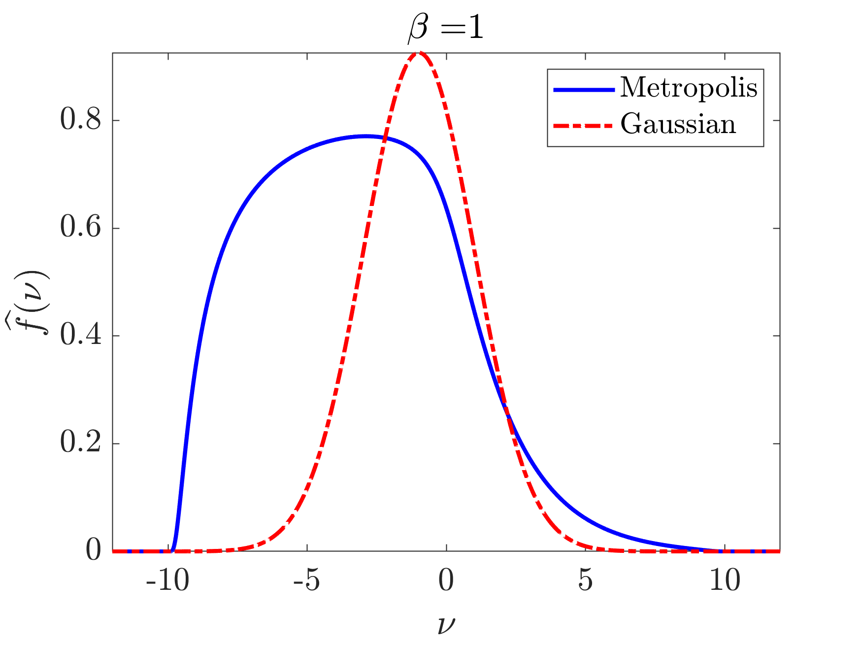
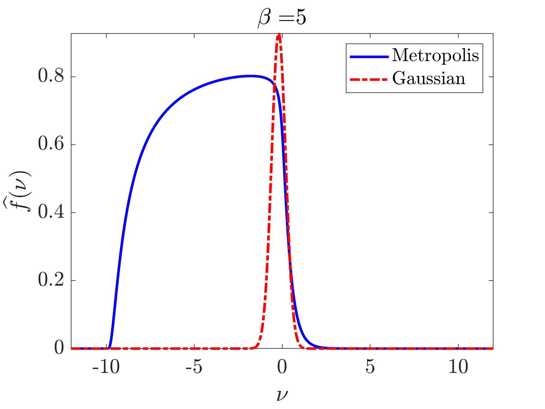
According to [AHR17, Corollary 2.8], for any , there exists a “bump function” such that and when . Here is an adjustable parameter to control the support of . Then is supported on and . Now we provide two specific examples of satisfying 15.
- •
-
•
Gaussian-type444In this case, the Gaussian functions already decay rapidly. The multiplication with a bump function is for purely technical reasons to ensure is compactly supported.:
(3.21) Here is a Gevrey function of order by [HR19, Proposition B.1] and the -integrability of its derivative is straightforward. So we still have . Setting , there holds
(3.22) which is approximately a Gaussian function concentrated at with width .
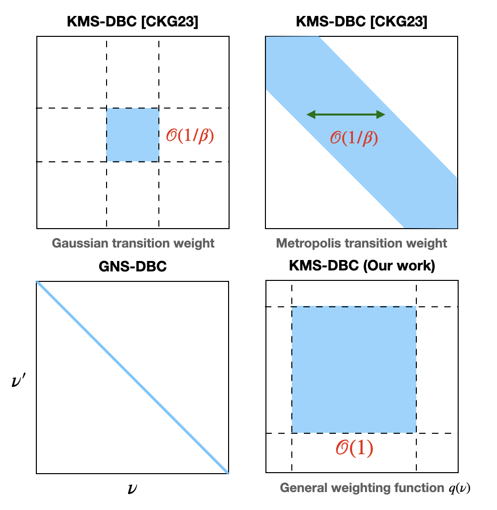
A comparison of the shapes of the Metropolis-type and Gaussian-type filtering function is shown in Fig. 1. The support size for the Gaussian choice decreases as , which can cause inefficiency because the magnitude of a local move in Monte Carlo simulations stays around order 1, regardless of the value of .
3.3. Efficient simulation of the Lindblad master equation (3.9)
In this section, we discuss the efficient simulation of the Lindblad equation in (3.9). For simplicity, we assume that , , and and satisfies 15. Our construction uses the block encoding input model and the linear combination of unitaries (see Appendices A and B). We also assume to ensure that efficient block encodings of are available (see Eq. 3.23).
Thanks to our algorithm’s use of a discrete set of jump operators for the Lindbladian, we can directly apply efficient Lindblad simulation quantum algorithms, such as those in [CW17, LW23, CKG23, DLL24], to prepare the Gibbs state, once the efficient constructions of the block encodings of and are available, which will be the focus of the rest of this section.
According to 16, in the following discussion, we set the integer large enough and consider the quadrature points () as in Eq. 3.13 such that Eq. 3.14 holds. Without loss of generality, we assume with .
For the quantum simulation, we assume access to the following oracles:
-
•
Block encoding of the coupling operators :
(3.23) We assume that the block encoding factor can be chosen to satisfy . Here represents the ancilla qubits utilized in the block-encoding of , is the identity matrix acts on the index register.
-
•
Controlled Hamiltonian simulations555The circuit construction is similar to the controlled Hamiltonian simulations in the standard quantum phase estimation, and the total Hamiltonian simulation time required is . for :
(3.24) -
•
Prepare oracle for , acting on the index register:
(3.25) which is used to implement LCU for the sum over in appearing in . Here are Hadamard gates acting the index register and are self-adjoint.
- •
- •
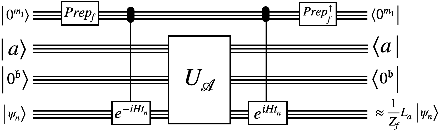
Using these oracles, according to 16, we can apply LCU with (3.23), (3.24), (3.26), and (3.27) to construct a
-block encoding of :
| (3.32) |
Here is defined in 16. The circuit of can be found in Fig. 2. In (3.32), the total Hamiltonian simulation time required by one query to is .
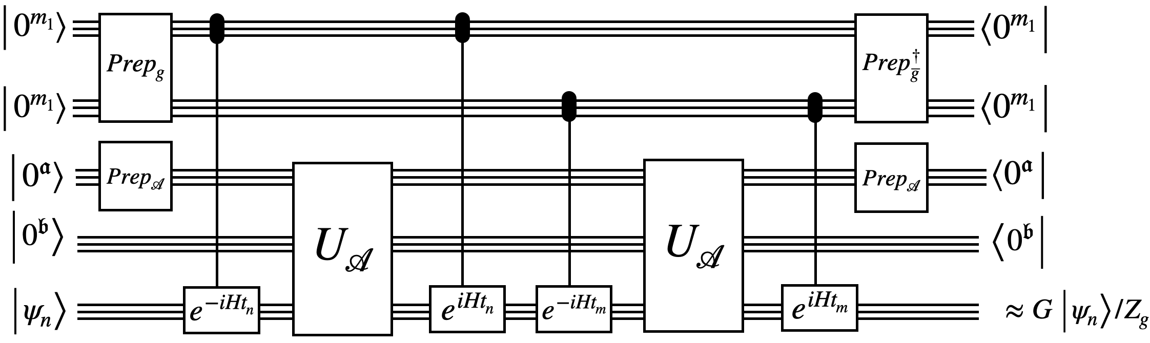
Next, applying two layers of LCU (see Appendix B) with (3.23), (3.24), (3.25), (3.29), and (3.30), we construct the following
-block encoding of :
| (3.33) | ||||
Here is defined in 16. We note that for and are acting on different time registers. The circuit of is given in Fig. 2. In (3.33), one query to still requires total Hamiltonian simulation time.
After acquiring the block encodings of and , we can employ the algorithm proposed in [LW23] to simulate (3.9). The complexity of this algorithm is recalled below.
Theorem 18 ([LW23, Theorem 11]).
Suppose that we are given an -block encoding of , and -block encodings for the jumps 666In [LW23], the authors assume separate access to the block encodings of . This is slightly different from our setting assuming the block-encoding of . . Let . For all with , there exists a quantum algorithm for simulating (3.9) up to time with an -diamond distance using
| (3.34) |
queries to and and
additional ancilla qubits.
Now, we are ready to give the simulation cost of our method as follows.
Theorem 19.
Assume access to weighting functions satisfying 15 with any , block encodings in Eq. 3.23, controlled Hamiltonian simulation in Eq. 3.24, and prepare oracles for filtering functions and in (3.26)–(3.30). The Lindbladian evolution (3.9) can be simulated up to time with an -diamond distance, and the total Hamiltonian simulation time is
where the constant is defined as follows:
In addition, the algorithm requires
number of additional ancilla qubits for the prepare oracles and simulation. The absorbs a constant only depending on and subdominant polylogarithmic dependencies on parameters , , , , , , and .
Remark 20.
In the above theorem, the total Hamiltonian simulation time scales quadratically in , a complexity seemingly less favorable compared to the one in [CKG23], which is only linearly dependent in (see Table 1). We will provide a detailed explanation of this distinction in Section 4. However, at first glance, we note that if is chosen as a concentrated filtering function with support width , one can readily recover a linear scaling of the total Hamiltonian simulation time in . Although this choice offers a better theoretical simulation complexity, it confines energy transitions to a narrow range, potentially prolonging the mixing time. Balancing this trade-off by selecting appropriately constitutes an intriguing avenue for future research.
Proof.
For simplicity, we let
| (3.35) |
By 18 with estimates in Eqs. 3.28 and 3.31, we have
| (3.36) | ||||
Recalling 16 and 32, we set a truncation time
| (3.37) |
and the step size
| (3.38) |
and then choose such that . This allows us to control the block-encoding error as follows:
Note that one query to the block encoding of requires one query to , by 18 and Eq. 3.36, the simulation requires
queries to . Similarly, we need
queries to . Combining this with the cost of one query to and , we can estimate the total Hamiltonian simulation time as follows:
Next, we consider the number of extra ancilla qubits, again by 18. We first note
and hence there holds
For the preparation oracles, by Eqs. 3.38 and 3.37, we find
This, along with Eqs. 3.16 and 3.18, implies that we need
additional ancilla qubits for the preparation of , , , and . Finally, requires ancilla qubits. Adding these quantities together concludes the proof. ∎
Remark 21.
In our simulation algorithm, thanks to the finite number of jump operators, we only need to construct the block encoding of for the efficient simulation. When , by assuming oracle access to a different form of blocking encodings of , we can simultaneously construct block encodings of all jump operators. Specifically, assuming oracle access to the block encoding of all coupling operators in the form , we can initially utilize [CKBG23, Appendix B.1 Lemma III.1] to construct a block encoding for and a block encoding for . Leveraging , we can implement the weak-measurement scheme proposed in [CKG23, Section III.1] to simulate (3.9) to first-order accuracy. Finally, by applying “compression” techniques as outlined in [CW17] to reduce the number of repetitions, the algorithm proposed in [CKG23, Appendix F] achieves optimal scaling in the number of uses of and .
4. Recovery of the Gibbs sampler in [CKG23]
In this section, we discuss the connections between our proposed family of efficient quantum Gibbs samplers with KMS DBC and those constructed in [CKBG23, CKG23] and show that our framework can recover the one in [CKG23].
We have seen from (2.16) that Davies generator (2.17) without the coherent term (i.e., Lindbladian with -GNS DBC) corresponds to the algorithmic Lindbladian (1.2) with and . As emphasized in 7, such a choice of Dirac delta filtering function for the frequency makes it hard to approximate GNS detailed balanced Lindblad dynamic. Chen et al. [CKBG23, Theorem I.3] introduced a Gaussian smoothed version by taking as
| (4.1) |
with of order , which guarantees that the Gibbs state is an approximate fixed point. It follows that the parameter has to be small enough so that , to prepare the Gibbs state accurately. Then [CKG23] carefully constructed coherent term such that the resulting dynamics is -KMS detailed balanced and could be a moderate constant, which reduced the computational cost significantly; see Table 1.
We next prove that our construction in Section 3 can include the one in [CKG23] as a special case. Let us first recall the construction by Chen, Kastoryano, and Gilyén. Suppose that is a given set of operators satisfying . [CKG23, Corollary II.2, Proposition II.4] defined the Lindbladian of the form (1.2):
| (4.2) | ||||
with the Gaussian filtering function (4.1) for , the Gaussian-type transition weight function:
| (4.3) |
or the Metropolis-type one:
| (4.4) |
and the Hamiltonian
| (4.5) |
Here, the coefficients are given by
| (4.6) |
We then define the so-called Kossakowski matrix [GKS76], which is a real and positive semidefinite matrix by choosing , to be non-negative functions. Then [CKG23] showed that if , there holds
| (4.7) |
which implies the KMS detailed balance of constructed in (4.2) [CKG23, Theorem I.1].
To proceed, for notational simplicity, we assume , which means that is a single self-adjoint operator . We introduce a new coefficient matrix:
| (4.8) |
which is real and positive semidefinite and satisfy the centrosymmetry by (4.7). We then consider the eigendecomposition of :
| (4.9) |
where is real orthogonal (hencd ) and is real diagonal with elements also indexed by . Moreover, by [CB76, Theorem 2], each eigenvector is either symmetric (namely, ) or skew-symmetric (namely, ). For , we define
| (4.10) |
Then, Eq. 4.2 can be reformulated as
and one can verify that and satisfy the requirements in 10.
For this, let us first consider defined in (4.5). Noting from the construction (4.10) that
we compute, according to (4.5),
| (4.11) |
which matches the general form (2.33). We next check the condition (2.28). We start with the case where is symmetric. By (2.21) and (4.10), it holds that
where we use and in the second equality. For the case where is skew-symmetric, a similar computation gives
where the third equality is by and .
Finally, to see that our construction in Section 3.1 recovers the quantum Gibbs sampler in [CKG23], it suffices to define the weighting function:
| (4.12) |
and find as required in (3.2) and that the jumps in (4.10) are the same as those in (3.4) with and given above.
Remark 22.
Letting be given as above, choosing to satisfy the KMS condition (2.20), in the limit , the matrix in (4.6) reduces to (up to some constant) and the associated Lindblad dynamic becomes GNS detailed balanced. One can similarly define the matrix as in (4.8) with decomposition (4.9). It holds that for each , there exists a symmetric eigenvector and a skew-symmetric one , which corresponds to the eigenvalue . In this case, in (4.12) is either or , and the jumps defined in (4.10) are consistent with those in (2.35).
We now estimate the element distribution of the Kossakowski matrix , which in principle determines the KMS detailed balanced Lindbladian, in view of Eqs. 4.2 and 4.5. This would help us better understand the effects of the choice of on the energy transition and how our proposed Gibbs sampler relates to those in [CKBG23, CKG23]. Recall the definition of in Eq. 4.6 and note that was chosen as a Gaussian . It follows that for any -bounded ,
where is a uniform constant. This means that for any fixed ,
| (4.13) |
that is, is concentrated around the diagonal part, which is the case for the Metropolis-type transition weight (4.4), due to for . When , this narrow strip shrinks rapidly and the matrix approximately reduces to a diagonal one so that the sampler becomes GNS detailed balanced (22). For the case of Gaussian transition weight (4.3), we can see that the is actually concentrated around the origin:
by the explicit computation in [CKG23, Proposition II.3]. In contrast, for our Gibbs sampler constructed in Section 3.1, we have
which is always supported on independent of by 15. We refer the readers to Fig. 3 below for an illustration of the pattern of for various Gibbs samplers.
Remark 23.
Recall 20 and note that in [CKG23], both choices of and in Eqs. 4.3 and 4.4 give the linear dependence of the total Hamiltonian simulation time on . The discrepancy in complexity between our approach and theirs arises from the difference in the construction of jump operators and coherent terms. The discussion above shows that when , (see Eq. 4.13). Consequently, in (4.2), the energy transition in is always close to the energy transition in . This property ensures that the norm of the coherent term in [CKG23] and the normalization block encoding constant does not increase linearly in . This differs from our case, where always includes a -sized principal submatrix and the dynamics allows different energy transition terms even when . Therefore, our coherent has much more cross terms in the expansion, and the normalization constant for the block encoding increases linearly in (3.31). This introduces an additional factor in our complexity result (see 19).
Conflict of interest statment
Authors have no conflict of interest to declare.
References
- [AC21] Érik Amorim and Eric A. Carlen. Complete positivity and self-adjointness. Linear Algebra Appl., 611:389–439, 2021.
- [ACL23] Dong An, Andrew M Childs, and Lin Lin. Quantum algorithm for linear non-unitary dynamics with near-optimal dependence on all parameters. arXiv preprint arXiv:2312.03916, 2023.
- [AGIK09] Dorit Aharonov, Daniel Gottesman, Sandy Irani, and Julia Kempe. The power of quantum systems on a line. Comm. Math. Phys., 287(1):41–65, 2009.
- [AHR17] Ziad Adwan, Gustavo Hoepfner, and Andrew Raich. Global -gevrey functions and their applications. J. Geom. Anal., 27:1874–1913, 2017.
- [Ali76] Robert Alicki. On the detailed balance condition for non-hamiltonian systems. Rep. Math. Phys., 10(2):249–258, 1976.
- [BCC+14] Dominic W Berry, Andrew M Childs, Richard Cleve, Robin Kothari, and Rolando D Somma. Exponential improvement in precision for simulating sparse hamiltonians. In STOC 2014, pages 283–292, 2014.
- [BCG+23] Ivan Bardet, Ángela Capel, Li Gao, Angelo Lucia, David Pérez-García, and Cambyse Rouzé. Rapid thermalization of spin chain commuting Hamiltonians. Phys. Rev. Lett., 130(6):060401, 2023.
- [BLMT24] Ainesh Bakshi, Allen Liu, Ankur Moitra, and Ewin Tang. High-Temperature Gibbs States are Unentangled and Efficiently Preparable. arXiv preprint arXiv:2403.16850, 2024.
- [Boy07] Khristo N. Boyadzhiev. Derivative polynomials for tanh, tan, sech and sec in explicit form. Fibonacci Quart., page 291–303, 2007.
- [BP02] Heinz-Peter Breuer and Francesco Petruccione. The theory of open quantum systems. OUP Oxford, 2002.
- [CB76] Antonio Cantoni and Paul Butler. Properties of the eigenvectors of persymmetric matrices with applications to communication theory. IEEE T COMMUN, 24(8):804–809, 1976.
- [CB21] Chi-Fang Chen and Fernando G.S.L. Brandão. Fast Thermalization from the Eigenstate Thermalization Hypothesis. arXiv preprint arXiv:2112.07646, 2021.
- [CKBG23] Chi-Fang Chen, Michael J. Kastoryano, Fernando G.S.L. Brandão, and András Gilyén. Quantum thermal state preparation. arXiv preprint arXiv:2303.18224, 2023.
- [CKG23] Chi-Fang Chen, Michael J. Kastoryano, and András Gilyén. An efficient and exact noncommutative quantum Gibbs sampler. arXiv preprint arXiv:2311.09207, 2023.
- [CLVBY24] Daan Camps, Lin Lin, Roel Van Beeumen, and Chao Yang. Explicit quantum circuits for block encodings of certain sparse matrices. SIAM J. Matrix Anal.Appl., 45(1):801–827, 2024.
- [CM17] Eric A. Carlen and Jan Maas. Gradient flow and entropy inequalities for quantum markov semigroups with detailed balance. J. Funct. Anal., 273(5):1810–1869, 2017.
- [CM20] Eric A. Carlen and Jan Maas. Non-commutative calculus, optimal transport and functional inequalities in dissipative quantum systems. J. Stat. Phys., 178(2):319–378, 2020.
- [Com74] L. Comtet. Advanced Combinatorics: The Art of Finite and Infinite Expansions. Springer Netherlands, 1974.
- [CS17] Anirban Narayan Chowdhury and Rolando D. Somma. Quantum algorithms for Gibbs sampling and hitting-time estimation. Quantum Inf. Comput., 17(1-2):41–64, 2017.
- [Cub23] Toby S. Cubitt. Dissipative ground state preparation and the dissipative quantum eigensolver. arXiv preprint arXiv:2303.11962, 2023.
- [CW12] Andrew M. Childs and Nathan Wiebe. Hamiltonian simulation using linear combinations of unitary operations. Quantum Inf. Comput., 12:901–924, 2012.
- [CW17] Richard Cleve and Chunhao Wang. Efficient quantum algorithms for simulating Lindblad evolution. In ICALP 2017, 2017.
- [Dav74] E. Brian Davies. Markovian master equations. Commun. Math. Phys., 39:91–110, 1974.
- [Dav76] E. Brian Davies. Quantum theory of open systems. Academic Press, 1976.
- [Dav79] E. Brian Davies. Generators of dynamical semigroups. J. Funct. Anal., 34(3):421–432, 1979.
- [DLL24] Zhiyan Ding, Xiantao Li, and Lin Lin. Simulating open quantum systems using hamiltonian simulations. arXiv preprint arXiv:2311.15533, 2024.
- [FS02] Daan Frenkel and Berend Smit. Understanding Molecular Simulation: From Algorithms to Applications. Academic Press, 2002.
- [FU07] Franco Fagnola and Veronica Umanità. Generators of detailed balance quantum Markov semigroups. Infin. Dimens. Anal. Quantum Probab. Relat. Top., 10(03):335–363, 2007.
- [FU10] Franco Fagnola and Veronica Umanità. Generators of KMS symmetric Markov semigroups on symmetry and quantum detailed balance. Commun. Math. Phys., 298(2):523–547, 2010.
- [GKS76] Vittorio Gorini, Andrzej Kossakowski, and Ennackal Chandy George Sudarshan. Completely positive dynamical semigroups of -level systems. J. Math. Phys., 17:821–825, 1976.
- [GSLW19] András Gilyén, Yuan Su, Guang Hao Low, and Nathan Wiebe. Quantum singular value transformation and beyond: exponential improvements for quantum matrix arithmetics. In STOC 2019, pages 193–204, 2019.
- [HR19] Gustavo Hoepfner and Andrew Raich. Global Gevrey Functions, Paley-Weiner Theorems, and the FBI Transform. Indiana University Mathematics Journal, 68(3):pp. 967–1002, 2019.
- [KB16] Michael J. Kastoryano and Fernando G.S.L. Brandão. Quantum Gibbs samplers: The commuting case. Commun. Math. Phys., 344:915–957, 2016.
- [KFGV77] Andrzej Kossakowski, Alberto Frigerio, Vittorio Gorini, and Maurizio Verri. Quantum detailed balance and KMS condition. Commun. Math. Phys., 57(2):97–110, 1977.
- [KSV02] Alexei Yu Kitaev, Alexander Shen, and Mikhail N. Vyalyi. Classical and quantum computation. Number 47 in Graduate Studies in Mathematics. American Mathematical Soc., 2002.
- [KT13] Michael J Kastoryano and Kristan Temme. Quantum logarithmic Sobolev inequalities and rapid mixing. J. Math. Phys., 54(5):1–34, 2013.
- [LC19] Guang Hao Low and Isaac L. Chuang. Hamiltonian simulation by qubitization. Quantum, 3:163, 2019.
- [Lid19] Daniel A. Lidar. Lecture notes on the theory of open quantum systems. arXiv preprint arXiv:1902.00967, 2019.
- [Lin76] Goran Lindblad. On the generators of quantum dynamical semigroups. Commun. Math. Phys., 48:119–130, 1976.
- [LW23] Xiantao Li and Chunhao Wang. Simulating Markovian Open Quantum Systems Using Higher-Order Series Expansion. In ICALP 2023, pages 87:1–87:20, 2023.
- [ML20] Evgeny Mozgunov and Daniel Lidar. Completely positive master equation for arbitrary driving and small level spacing. Quantum, 4(1):1–62, 2020.
- [NKL22] Quynh T. Nguyen, Bobak T. Kiani, and Seth Lloyd. Block-encoding dense and full-rank kernels using hierarchical matrices: applications in quantum numerical linear algebra. Quantum, 6:876, 12 2022.
- [Pin08] Mark A. Pinsky. Introduction to Fourier Analysis and Wavelets. Graduate studies in mathematics. American Mathematical Society, 2008.
- [PW09] David Poulin and Pawel Wocjan. Preparing ground states of quantum many-body systems on a quantum computer. Phys. Rev. Lett., 102(13):130503, 2009.
- [RFA24] Cambyse Rouzé, Daniel Stilck Franca, and Álvaro M. Alhambra. Efficient thermalization and universal quantum computing with quantum Gibbs samplers. arXiv preprint arXiv:2403.12691, 2024.
- [RWW23] Patrick Rall, Chunhao Wang, and Pawel Wocjan. Thermal state preparation via rounding promises. Quantum, 7:1132, 2023.
- [SCC23] Christoph Sünderhauf, Earl Campbell, and Joan Camps. Block-encoding structured matrices for data input in quantum computing. arXiv preprint arXiv:2302.10949, 2023.
- [SM23] Oles Shtanko and Ramis Movassagh. Preparing thermal states on noiseless and noisy programmable quantum processors. arXiv preprint arXiv:2112.14688, 2023.
- [TKR+10] Kristan Temme, Michael James Kastoryano, Mary Beth Ruskai, Michael Marc Wolf, and Frank Verstraete. The -divergence and mixing times of quantum Markov processes. J. Math. Phys., 51(12), 2010.
- [TOV+11] Kristan Temme, Tobias J. Osborne, Karl G. Vollbrecht, David Poulin, and Frank Verstraete. Quantum Metropolis sampling. Nature, 471(7336):87–90, 2011.
- [VAGGdW17] Joran Van Apeldoorn, András Gilyén, Sander Gribling, and Ronald de Wolf. Quantum SDP-solvers: Better upper and lower bounds. In FOCS 2017, pages 403–414. IEEE, 2017.
- [Wol12] Michael M. Wolf. Quantum channels & operations: guided tour. Lecture Notes. URL http://www-m5. ma. tum. de/foswiki/pub M, 2012.
- [WT23] Pawel Wocjan and Kristan Temme. Szegedy walk unitaries for quantum maps. Commun. Math. Phys., 402(3):3201–3231, 2023.
- [YAG12] Man-Hong Yung and Alán Aspuru-Guzik. A quantum–quantum Metropolis algorithm. PNAS, 109(3):754–759, 2012.
- [ZB23] Yikang Zhang and Thomas Barthel. Criteria for Davies irreducibility of Markovian quantum dynamics. J. Phys. A: Math. Theor, 2023.
Appendix A Block encoding
Block encoding (see [LC19, GSLW19]) provides a general framework for encoding a non-unitary matrix using unitary matrices, which can be implemented on quantum devices.
Definition 24 (Block encoding).
Given a matrix , if we can find , and a unitary matrix so that
| (A.1) |
then is called an -block-encoding of . The parameter is referred to as the block encoding factor, or the subnormalization factor.
Intuitively, the block encoding matrix encodes the rescaled matrix in its upper left block:
There have been substantial efforts on implementing the block encoding of certain structured matrices of practical interest [GSLW19, NKL22, CLVBY24, SCC23]. In this work, we assume that the query access to the block encoding of relevant matrices is available. We also assume that there is no error in the block encodings of the input matrices , , etc. If such errors are present, their impact should be treated using perturbation theories. Meanwhile, we need to carefully keep track of the error of the block encodings derived from the input matrices, such as the jump operators .
Appendix B Linear combination of unitaries
The linear combination of unitaries (LCU) [CW12] is an important quantum primitive, which allows matrices expressed as a superposition of unitary matrices to be coherently implemented using block encoding. Here we follow [GSLW19] and present a general version of the LCU that is applicable to possibly complex coefficients.
LCU implements a block encoding of , where are unitary operators and are complex numbers. For the coefficients, we assume access to a pair of state preparation oracles (also called prepare oracles for short) acting as (assume )
Here the coefficients should satisfy . To minimize the block encoding factor, the optimal choice is , and where refers to the principal value of the square root of . In this case, , where is the -norm of the vector .
The unitaries needs to be accessed via a select oracle Select as
which can be constructed using controlled versions of the block encoding matrices .
Lemma 25 (LCU).
Assume , , then the matrix
is a -block-encoding of the linear combination of unitaries .
Appendix C Gevrey functions
In this section, we collect a few results for Gevrey functions that are useful for this work. While similar findings have been previously demonstrated in the literature, notably in [AHR17] and [HR19], we provide self-contained proofs here with explicit expressions for the constants involved.
Lemma 26 (Product of Gevrey functions).
Given and , then
Proof.
For a index vector , a direct application of Leibniz rule gives
where the third inequality is by . ∎
We next show that is a Gevrey function and its derivative is -integrable. We first recall the Faà di Bruno’s formula and the partial Bell polynomial for the chain rule of high-order derivatives [Com74, p.139].
Lemma 27 (Faà di Bruno’s formula and partial Bell polynomial).
Let be smooth function from to , and . Then the -th order derivative of is given by
where the sum is over all -tuples of nonnegative integers satisfying . The above formula can also be rewritten as
where is the partial Bell polynomial:
Using Faà di Bruno’s formula, we can calculate the high order derivatives of and verify that it belongs to a Gevrey class.
Lemma 28.
It holds that
Proof.
We first use the second formula of 27 and some properties of the partial Bell polynomials to calculate -th order derivative for . For , we have (define if )
Using the fact that , , and , we have
Next, by Faà di Bruno’s formula for , we obtain
| (C.1) | ||||
Plugging the upper bound gives
where we use the fact that the number of -tuples of nonnegative integers satisfying is less than . This concludes . The -integrablity of is a simple consequence of Eq. C.1. ∎
Finally, we show that the Fourier transform of the Gevrey class with compact support decays rapidly, by a Paley-Wiener type estimate.
Lemma 29.
Given with compact support and , define
Then, for any , there holds
where is the volume of and is the -norm of the vector .
Appendix D Quadrature error analysis
In this section, for notational simplicity, sometimes we absorb the generic constant depending on the parameter of the filtering function in Eq. 3.12 into . We first study the decaying and integrable property of the functions and .
Lemma 30.
Proof.
We recall the definitions of and :
| (D.5) |
and
| (D.6) |
Exponential decay of . Thanks to 26 with 15, we have
Then, 29 with and yields the estimate for :
| (D.7) |
Exponential decay of . By using [Boy07, Eq. (3.3)], we first have
which implies
| (D.8) |
It follows from 26 with
that
Again, applying 29 with and gives
| (D.9) |
which concludes the proof for the decay of .
Estimate the integral of . We note from 15 that the derivative of is -integrable. It follows that
and then
by the invariance of in . Here, we use and to obtain . In addition, because , there holds
Thus, we readily have, for any ,
| (D.10) | ||||
Next, by Eq. D.1, a direct computation via change of variable gives
| (D.11) |
We define the constant by
| (D.12) |
which satisfies the following asymptotics: as ,
Note that is decreasing on and increasing on with global minimum at . For any , the equation has a unique solution , which readily gives and thus, by (D.12),
| (D.13) |
We can then estimate the integral by Eqs. D.10 and D.11, as well as Eq. D.13,
| (D.14) | ||||
for any positive . This gives Eq. D.3.
Estimate the integral of . Similarly, by Eq. D.6 with 15 and , we have . A direct computation gives, for a fixed ,
with its and norms independent of . This implies
In addition, we have the second-order partial derivative:
which is -integrable in (for fixed ). Then, we can estimate
by a straightforward computation:
In the same manner as Eq. D.10, we have
| (D.15) |
We next prove 16. We shall employ the Poisson summation formula recalled in the following lemma [Pin08, Theorem 4.4.2].
Lemma 31 (Poisson summation formula).
Given any with inverse Fourier transform:
for any and , there holds
We are now ready to show 16.
Proof of 16.
In the proof, we shall consider an infinite time grid defined by . The grid is given by the subset as in the statement of 16. We omit the upper index in and .
Estimate for the jump . Thanks to 30, there holds
| (D.17) | ||||
By the monotonicity of the exponential function, we have
| (D.18) | ||||
Let be the constant defined as in Eq. D.12. Then, when , we can compute, by (D.18),
Combining this with Eq. D.17, we find
| (D.19) | ||||
Then, by the triangle inequality, we readily have
| (D.20) | ||||
with constant
Note from (3.4) that , and from 15 that
For , by Poisson summation formula in 31, we have
Plugging the above formula into the first term of (D.20), there holds
which then implies
and concludes the proof of (3.15).
Estimate for the coherent term . Again by 30 with similar estimates as in (D.19) for , we obtain, when ,
where the constant is given in Eq. D.16 and
It follows that
| (D.21) | ||||
Similarly, Poisson summation formula with gives
for and , thanks to . It follows that the first term of (D.21) is zero. By definition (3.7) of and above estimates, it holds that
The proof is complete. ∎
Finally, the simulation of the algorithm requires the preparation of oracles (3.26)-(3.30), where the normalization factors and affect the algorithm complexity. In the following theorem, we demonstrate that the discretization normalization constant can be bounded by the norm of and when the discretization step is sufficiently small.