Active quantum flocks

Abstract

Flocks of animals represent a fascinating archetype of collective behavior in the macroscopic classical world, where the constituents, such as birds, concertedly perform motions and actions as if being one single entity. Here, we address the outstanding question of whether flocks can also form in the microscopic world at the quantum level. For that purpose, we introduce the concept of active quantum matter by formulating a class of models of active quantum particles on a one-dimensional lattice. We provide both analytical and large-scale numerical evidence that these systems can give rise to quantum flocks. A key finding is that these flocks, unlike classical ones, exhibit distinct quantum properties by developing strong quantum coherence over long distances. We propose that quantum flocks could be experimentally observed in Rydberg atom arrays. Our work paves the way towards realizing the intriguing collective behaviors of biological active particles in quantum matter systems. We expect that this opens up a path towards a yet totally unexplored class of nonequilibrium quantum many-body systems with unique properties.

In the quantum world, remarkable advances in quantum simulators have led to unprecedented capabilities in controlling and probing the real-time dynamics of quantum matter Gross and Bloch (2017); Monroe et al. (2021); Browaeys and Lahaye (2020); Blais et al. (2021). Among the most important developments have been the observation of genuinely nonequilibrium phases of matter such as many-body localization Schreiber et al. (2015); Smith et al. (2016), discrete time crystals Choi et al. (2017); Zhang et al. (2017), or quantum many-body scars Bernien et al. (2017). In the classical world, progress in the understanding of dynamical processes maintained away from equilibrium in the context of active matter systems, e.g. describing the physics of biological systems, has been distinctly impressive Jülicher et al. (1997); Ramaswamy (2010); Marchetti et al. (2013); Prost et al. (2015); Cates and Tjhung (2018); Weber et al. (2019). This, in particular, includes one of the most fascinating archetypes of collective motion - flocks, which realize an oriented, clustered, and moving collection of constituents Vicsek et al. (1995); Toner et al. (2005); Chaté (2020). So far, these developments on the nonequilibrium many-body physics of quantum and classical systems have evolved independently, leaving open the fundamental question emerging naturally at their interface: is it also possible for quantum particles to exhibit flocking, similar to birds or fish in the classical world?

In this work, we first introduce the concept of active quantum matter by formulating fundamental dynamical processes for the involved quantum particles. We then provide evidence that these particles can realize a quantum flock in that they form collectively moving clusters which spontaneously undergo polar symmetry breaking. We observe that the resulting flock experiences distinct quantum features absent in the classical world. Specifically, our active quantum system exhibits a pronounced long-ranged quantum coherence suggesting coherent, ballistic motion over large distances. We argue that the identified underlying mechanism is general and can be potentially used to realize also other phases of active quantum matter. Our work therefore opens up a route towards exploring yet unknown classes of nonequilibrium states in quantum many-body systems, with the possibility to materialize on the fascinating collective behaviors of biological active matter systems in a quantum context. We expect that this provides a path to a multitude of potential nonequilibrium quantum phases to be explored in the future.

Model for active quantum flocks

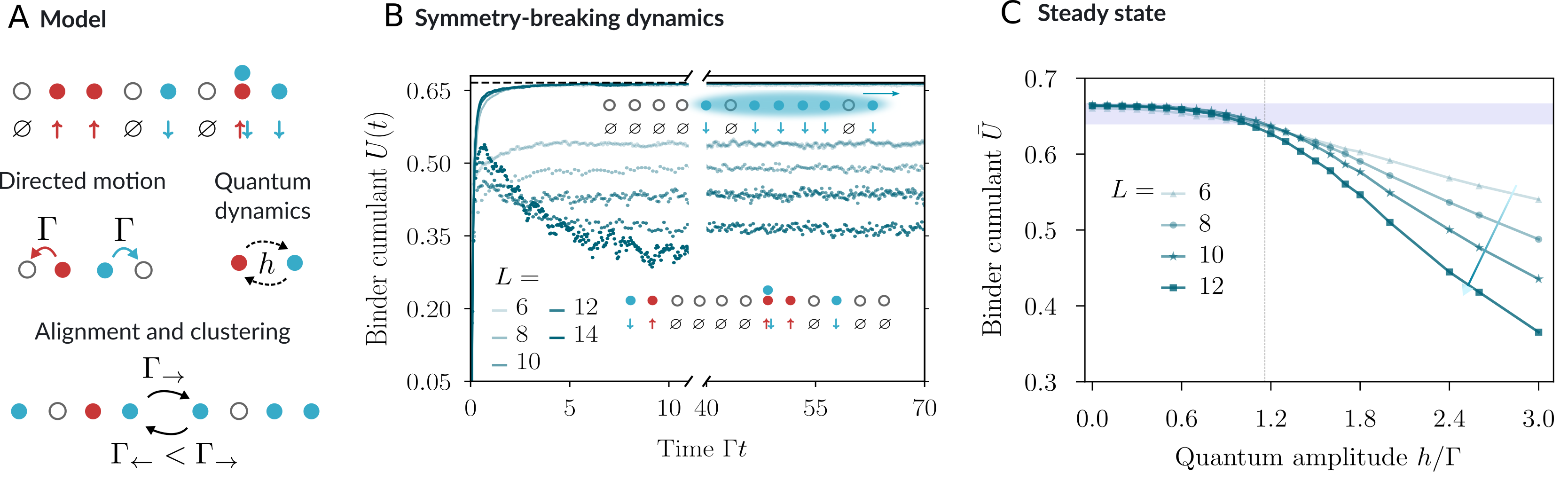
Figure 1: Active quantum flocks. A The introduced model for active quantum matter involves two species of hard-core bosons ($\uparrow,\downarrow)$ on a one-dimensional lattice subject to three types of dynamical processes. The particles perform a dissipative directed motion at a rate $\Gamma$ with $\uparrow$ and $\downarrow$ particles moving to the left and right, respectively. Quantum dynamics is introduced by a coherent spin-flip process occurring with an amplitude $h$. Alignment and clustering of particles is enabled by a conditional dissipative spin-flip process whose rate effectively depends on the surrounding magnetization. Here, the rate $\Gamma_{\leftarrow}<\Gamma_{\rightarrow}$ as the environment is dominated by $\downarrow$ particles. B Dynamics of the Binder cumulant $U(t)$ for different quantum amplitudes $h$. For weak $h=0.2$ (solid lines) the Binder cumulant approaches a value of $U=2/3$ for large system sizes $L$ indicative of symmetry breaking and long-range order, whereas for large $h=3.0$ (dotted lines) the Binder cumulant exhibits a tendency towards a vanishing value upon increasing $L$ suggesting a disordered phase. The numerical data has been obtained for an alignment parameter $K=3.8$ and $N_{r}=1000$ trajectories. C Long-time average of the Binder cumulant $\overline{U}$ as a function of the strength $h$ of the quantum dynamics for different system sizes $L$ at alignment parameter $K=3.8$. For weak $h$ the Binder cumulant approaches a value of $U=2/3$ indicative of symmetry breaking and therefore of a quantum flocking phase, whereas for large $h$ the Binder cumulant displays a tendency towards a vanishing value upon increasing $L$. The horizontal shaded area indicates the threshold used to estimate the phase transition point, which is included as the dashed line. For the numerical data we have used $N_{r}=1000$ trajectories.

It is the key aim of this work to devise a quantum-mechanical analogue of active matter systems Solon and Tailleur (2013, 2015), with the particular goal to realize flocks in the quantum world. The central feature of active particles is that their motion is continuously supplied with energy on the single-particle level from an environment Ramaswamy (2010); Marchetti et al. (2013); Weber et al. (2014); Fodor et al. (2022); Bär et al. (2020), breaking local detailed balance and enabling persistent motion. In order for such active particles to form a flock, a so-called alignment process is required describing an interaction which correlates the particles direction of motion according to their environment, such as birds aligning their velocity with their neighbors’ in the pioneering Vicsek model Vicsek et al. (1995).

When turning to the quantum world, we are, however, facing two key challenges. On the one hand, it is unknown which environments can generate microscopic processes making a many-body system of quantum particles active by breaking local detailed balance. On the other hand, on a fundamental level, it is impossible to directly translate the local alignment of velocities as in the Vicsek model, since, quantum mechanically, positions and velocities (or momenta) are non-commuting observables.

In the following, we introduce a general class of quantum models resolving the challenges along both of these axes. We consider a system of hard-core bosons on a one-dimensional chain of $L$ lattice sites with periodic boundary conditions and two species of particles labeled by an effective spin $\sigma=\uparrow,\downarrow$, see Fig. 1A. In Supplementary Information Sec. III, we discuss how to realize the individual dynamical processes microscopically in systems of Rydberg atoms.

It is key for active matter to include dissipative processes. We choose environments that can be effectively described by a Lindblad master equation Gardiner and Zoller (2004):

$$\frac{d\hat{\rho}}{dt}=-i[\hat{H},\hat{\rho}]+{\cal D}(\hat{\rho})~{}\,.$$ (1)

which appear genuinely when coupling quantum matter to photons as the quanta of light. Here, $\hat{\rho}$ denotes the density matrix of the quantum system. Two types of contributions can be distinguished: the coherent evolution by the Hamiltonian $\hat{H}$, and the dissipative dynamics via $\mathcal{D}(\hat{\rho})$.

We now introduce specific environments, which realize the aforementioned two key desired processes responsible, firstly, for the active motion (labeled by $\mathcal{M}$) and, secondly, for the alignment ($\mathcal{A}$). This leads to a decomposition $\mathcal{D}(\hat{\rho})=\mathcal{D}_{\mathcal{M}}(\hat{\rho})+\mathcal{D}_{\mathcal{A}}(\hat{\rho})$, where ${\cal D}_{X}(\hat{\rho})=\sum_{l=1}^{L}\sum_{\sigma=\uparrow,\downarrow}(\Gamma_{X}/2)(2\hat{X}_{l\sigma}\hat{\rho}\hat{X}^{\dagger}_{l\sigma}-\hat{X}^{\dagger}_{l\sigma}\hat{X}_{l\sigma}\hat{\rho}-\hat{\rho}\hat{X}^{\dagger}_{l\sigma}\hat{X}_{l\sigma})$. Here, $X=\mathcal{M},\mathcal{A}$, and $\hat{X}_{l\sigma}$ denotes the respective quantum jump operator of species $\sigma$ on lattice site $l$ and $\Gamma_{X}$ is the rate of the corresponding process.

In order to break detailed balance locally and thereby make the system active, we choose quantum jump operators $\hat{\mathcal{M}}_{l\uparrow}=\hat{c}^{\dagger}_{l\uparrow}\hat{c}_{l+1\uparrow},~{}\hat{\mathcal{M}}_{l\downarrow}=\hat{c}^{\dagger}_{l+1\downarrow}\hat{c}_{l\downarrow}$. Here, $\hat{c}_{l\sigma}^{\dagger}$ denotes the creation operator for a hard-core boson of type $\sigma$ at lattice site $l$. This contribution leads to a directed motion of spin-$\uparrow$ and $\downarrow$ particles to the left and right, respectively, in close analogy to classical active Ising models Solon and Tailleur (2013, 2015). We show in Methods Sec. B that this dynamical process violates Kolmogorov’s criterion implying the breaking of local detailed balance, see also Extended Data Fig. 1. While recent works have already been aiming at identifying active quantum processes for single particles Zheng and Löwen ; Yamagishi et al. , the process presented here induces activity on a many-body level.

In a next step we now aim to address the challenge to realize a local alignment of velocities, which cannot be realized directly quantum mechanically. Instead, we achieve this indirectly by introducing a dissipative process aligning the internal degree of freedom $\sigma$. This $\sigma$ is linked to a direction of motion due to the active process, yielding the desired alignment. Concretely, we choose $\hat{\mathcal{A}}_{l\sigma}=\hat{c}^{\dagger}_{l\sigma}\hat{c}_{l\overline{\sigma}}\hat{P}_{l}~{}$ inducing transitions between the two particle species. Here, $\overline{\sigma}$ denotes the spin species with opposite orientation to $\sigma$. The key alignment property is contained in $\hat{P}_{l}$ which is designed to make the process conditional on a surrounding magnetization. This can be achieved for various variants of $\hat{P}_{l}$ (see Supplementary Sec. II). In the following, we use $\hat{P}_{l}=\mathrm{exp}(-K/(2r)\hat{m}_{l}\sum_{|j|=1}^{r}\hat{m}_{l+j})$ with $K$ denoting the alignment parameter and $r$ defining the interaction radius, which we choose as $r=4$ in the following. Here, $\hat{m}_{l}=\hat{n}_{\uparrow l}-\hat{n}_{\downarrow l}=\hat{c}^{\dagger}_{\uparrow l}\hat{c}_{\uparrow l}-\hat{c}^{\dagger}_{\downarrow l}\hat{c}_{\downarrow l}$ measures the local magnetization. In analogy to the Vicsek model Vicsek et al. (1995), where each point-agent aligns its velocity direction to the average direction of motion of its neighborhood, our quantum particles align according to their surrounding magnetization.

The Hamiltonian contributes the quantum-coherent real-time evolution through a local spin-flip term $\hat{H}=-h\sum_{l=1}^{L}\big{(}\hat{c}_{l,\uparrow}^{\dagger}\hat{c}_{l,\downarrow}+h.c\big{)}$ with $h$ denoting the quantum amplitude. Although the induced quantum dynamics counteracts the formation of a flock, we find, importantly, that it also qualitatively determines the character of the collective flock motion inducing a long-ranged quantum coherence absent in the classical case.

A key property of the considered model is a $\mathbb{Z}_{2}$-symmetry by flipping the spins of all particles upon simultaneously reversing the particles’ direction of motion, with the corresponding transformation $\hat{c}_{l\sigma}\mapsto\hat{c}_{(m-l)\overline{\sigma}}$ and $m$ any lattice site. This symmetry, which will be broken spontaneously in the quantum flock, couples the motion of particles to their spin degree of freedom. Consequently, collective motion of particles is detectable through the magnetization $\hat{M}=\sum_{l=1}^{L}\hat{m}_{l}$ as the order parameter.

We solve the resulting Lindblad master equation via exact diagonalization through a mapping to a stochastic Schrödinger equation (see Methods Sec. A). We achieve up to $L=14$ lattice sites, which corresponds for a single spin species to a large-scale system of $28$ lattice sites. On the level of the Lindblad equation this corresponds to solving the kinetics of a system governed by $10^{12}$ coupled first-order differential equations. In our simulations, we choose for convenience $\Gamma_{\mathcal{M}}=\Gamma_{\mathcal{A}}=\Gamma$, and we consider initial conditions $|\psi_{0}\rangle$ with a vanishing magnetization and short-range correlations: $|\psi_{0}\rangle=\otimes_{l=1}^{N}|\psi_{0}\rangle_{l}\otimes_{l=N+1}^{L}\ket{0}_{l}$, where $|\psi_{0}\rangle_{l}=2^{-1/2}(\ket{\uparrow}_{l}+\ket{\downarrow}_{l})$ and $|0\rangle_{l}$ denotes an empty lattice site. We verified that the properties of the steady state do not depend on the choice of the initial condition (see Supplementary Sec. III). The initial condition sets the density $\nu=N/L=1/2$ of particles in the system.

Long-range order and collective motion

We target the detection of long-range order by means of the Binder cumulant $U(t)=1-\langle\hat{M}^{4}(t)\rangle/(3\langle\hat{M}^{2}(t)\rangle^{2})$ associated to the order parameter $\hat{M}$. Here, $\langle\hat{\mathcal{O}}(t)\rangle=\mathrm{Tr}(\hat{\rho}(t)\hat{\mathcal{O}})$ denotes the time-dependent expectation value of the operator $\hat{\mathcal{O}}$. A more direct measure and visualization of the the quantum flock by means of snapshot measurements we introduce below. In the thermodynamic limit, the Binder cumulant is $U=2/3$ for long-range ordered states whereas $U=0$ for disordered ones. Note that the order parameter $\langle\hat{M}(t)\rangle=0$ itself remains zero throughout the dynamics due to the absence of any explicit symmetry-breaking contribution.

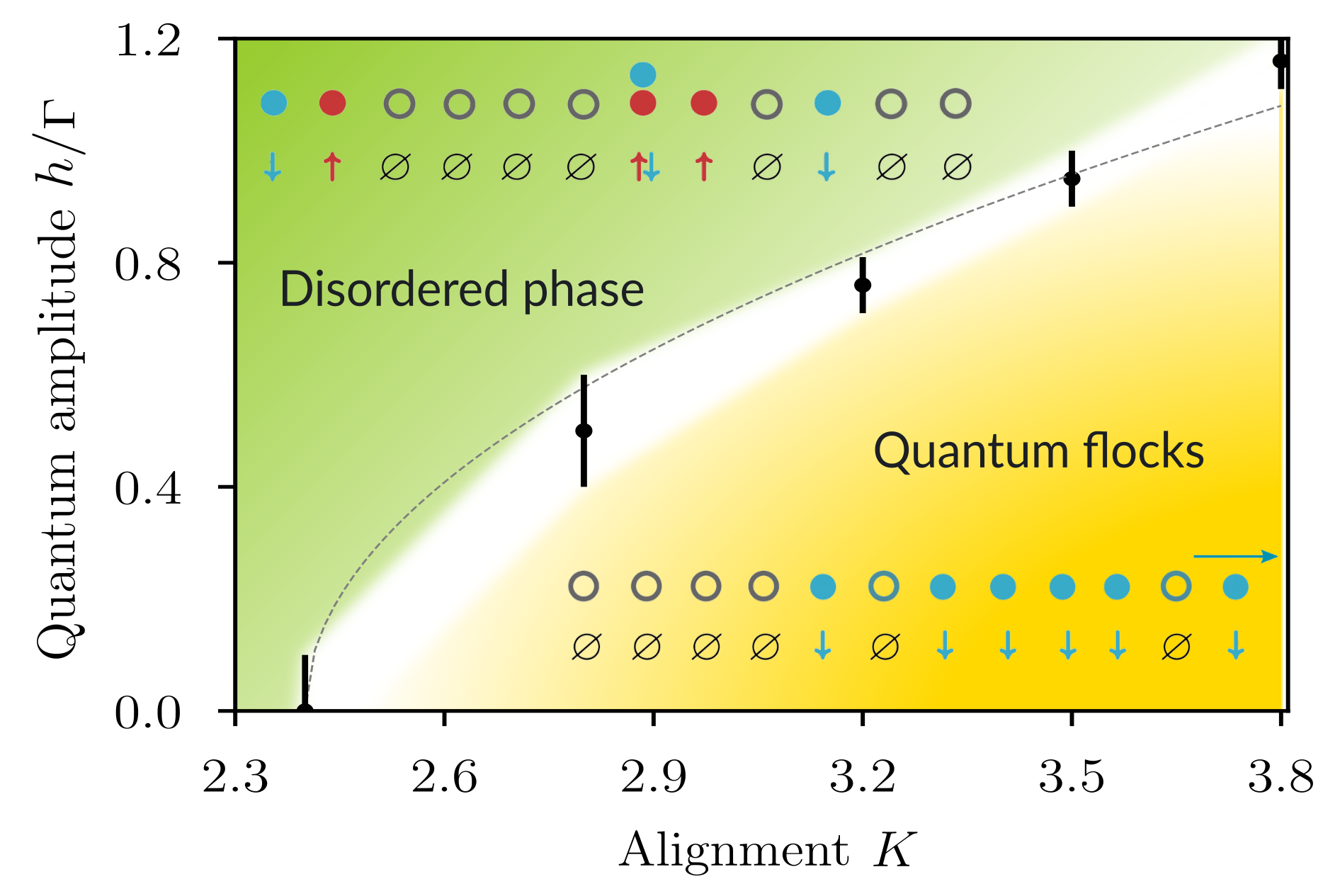
Figure 2: Phase diagram. Numerically obtained phase diagram with indicated error bars as a function of the alignment parameter $K$ and the quantum amplitude $h$ including representative many-body configurations. The numerical uncertainty for the estimate of the phase transition points is indicated by the white region separating the disordered from the quantum flocking phase. The analytical prediction from the coarse-grained theory at weak quantum amplitudes $h$ is included as a dashed line, which is consistent with the numerical results.

In Fig. 1B, we display numerically obtained data for the Binder cumulant $U(t)$. We observe qualitatively different behavior depending on the quantum amplitude $h$. For weak $h/\Gamma=0.2$, the Binder cumulant rises up to $U(t)\approx 2/3$ for long times with only weak finite-size effects. These results suggest long-range order and the realization of an active quantum flock experiencing collective motion. The behavior is different in the opposite case of large quantum amplitudes $h$ where the attained long-time value exhibits a considerable system-size dependence with $U\to 0$ upon increasing $L$, indicating a disordered phase.

In Fig. 1C, we show the long-time value $\overline{U}$ of the Binder cumulant as a function of $h$, obtained from a time average in the interval $\Gamma t\in[40,70]$. We observe compelling evidence for a long-range ordered phase at weak quantum amplitudes $h/\Gamma\ll 1$. For large quantum amplitudes instead the tendency is clearly towards a disordered state with $\overline{U}\to 0$ upon increasing $L$. We estimate the phase transition point by identifying the value of $h$ at which $\overline{U}$ crosses a threshold $2/3-\epsilon$ with $\epsilon=0.02$, as indicated also in Fig. 1C. The corresponding estimated phase diagram is shown in Fig. 2.

Quantum coherence

A key question remains, namely to what extent quantum flocks differ from the classical world. Characterizing such differences is a challenging task especially in mixed states of quantum matter. Instead of using quantum entanglement, we target this challenge by quantifying quantum coherence Streltsov et al. (2017), which we interpret as one of the most fundamental quantum properties in dynamical processes. Concretely, we consider the total long-distance quantum coherence $C(t)=\sum_{l=1}^{L}C_{l}(t)$ with $C_{l}(t)=\sum_{\nu_{l}\not=\nu^{\prime}_{l}}\big{|}\langle\nu_{l}|\hat{\rho}_{l}^{C}(t)|\nu^{\prime}_{l}\rangle\big{|}$, where $\hat{\rho}_{l}^{C}(t)$ denotes the reduced density matrix of two lattice sites $l$ and $l+L/2$, i.e., at a maximal distance. The states $|\nu_{l}\rangle=|\mathbf{n}_{l},\mathbf{n}_{l+L/2}\rangle$ represent all the particle configurations with $\mathbf{n}_{l}=\varnothing,\uparrow,\downarrow,\uparrow\downarrow$. In the absence of quantum superposition, i.e., for a vanishing quantum amplitude $h=0$, $C(t)=0$ for all times consistent with classical time evolution as one might expect due to the purely dissipative dynamics.

In Fig. 3A, we show our obtained numerical results for $C(t)$ at some fixed quantum amplitude $h/\Gamma=0.2$. In the disordered phase for weak alignment $K=0.5$, $C(t)$ settles to a plateau independent of system size $L$. In the flocking phase instead for large alignment $K=3.8$, $C(t)$ grows with increasing system size $L$ and time $t$. Consequently, the flock exhibits distinct quantum properties through a long-ranged quantum coherence.

The obtained results for $C(t)$ also have direct implications on the nature of the collective motion. $C(t)$ is a measure on the strength of the off-diagonal matrix elements in $\rho_{l}^{C}(t)$, which involve correlation functions of the form $\langle\hat{c}_{l\uparrow}^{\dagger}(t)\hat{c}_{l+L/2\uparrow}(t)\rangle$ for instance. This suggests that the flocking state is not only characterized by quantum superposition but also by long-distance quantum-coherent motion.

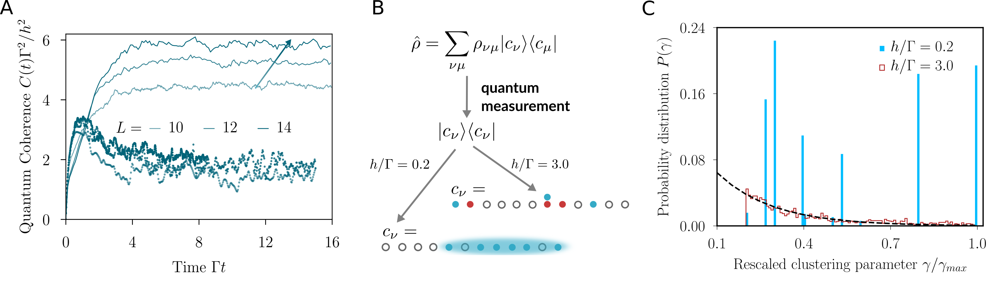
Figure 3: Quantum coherence and cluster formation. A Dynamics of the total long-distance quantum coherence $C(t)$ comparing the flocking phase ($K=3.8$, solid lines) to the disordered phase ($K=0.5$, dotted lines) for $h/\Gamma=0.2$ and different system sizes $L$. For strong alignment $K=3.8$ the flock exhibits a strong quantum coherence and quantum coherent motion over long distances. For the numerical calculations we have used $N_{r}=1000$ trajectories. B A quantum snapshot measurement on the full density matrix $\hat{\rho}$ yields many-body configurations $c_{\nu}$. Typical outcomes of such snapshots for the quantum flock ($h/\Gamma=0.2$) and for the disordered phase ($h/\Gamma=3.0$) are included. C Cluster statistics after many snapshot measurements comparing the quantum flock ($h/\Gamma=0.2$) to the disordered phase ($h/\Gamma=3.0$). The histogram of $\gamma$ at alignment parameter $K=3.8$ has been obtained for $N_{r}=2000$ trajectories and $L=12$. Here, $\gamma_{\text{max}}=L^{2}/4$ denotes the maximally possible $\gamma$ value.

Alignment and clustering

Having found evidence for intrinsic quantum effects, we aim in a next step to characterize the quantum flock on a microscopic level. For that purpose we introduce a method to extract its clustering structure by extending a clustering algorithm Rodriguez and Laio (2014) to snapshot measurements. Such snapshots are obtained by performing a joint projective quantum measurement on each lattice site providing as the outcome a single many-body configuration, as accessible on today’s quantum simulation or computing platforms Gross and Bloch (2017); Monroe et al. (2021); Browaeys and Lahaye (2020); Blais et al. (2021). Typical snapshots, determined from our exact numerics, are depicted in Fig. 3B pointing towards a fundamental difference between the flocking and disordered phases. Without loss of generality, we focus on the $\downarrow$-species with corresponding many-body configurations $\mathbf{n}=(n_{1\downarrow},n_{2\downarrow},\dots,n_{L\downarrow})$ and $n_{l\downarrow}=0,1$.

Within the utilized clustering algorithm Rodriguez and Laio (2014), a clustering parameter $\gamma_{l}=\varrho_{l}\delta_{l}$ is associated to each lattice site $l$. Here, $\varrho_{l}=n_{l\sigma}\sum_{|m-l|<d_{c}}n_{m\sigma}$ denotes a coarse-grained local density and $\delta_{l}=\min_{m\mathrel{\mathop{\mathchar 58\relax}}\varrho_{m}>\varrho_{l}}(|l-m|)$ measures the distance to the next lattice site with higher density. Large clusters can be identified through large values of $\gamma$ as they exhibit both a high local density $\varrho_{l}$ and a large distance $\delta_{l}$ Rodriguez and Laio (2014). In what follows, we choose $d_{c}=4$ for concreteness and for the site with the highest density we have $\delta_{l}=L/2$.

In Fig. 3C, we display the statistics of the clustering parameter $\gamma$ with $P(\gamma)$ obtained from a histogram. $P(\gamma)$ displays a compelling difference between the two phases. In the disordered domain for large quantum amplitudes $h/\Gamma=3$, we find that $P(\gamma)$ exhibits a monotonically decaying behavior. Thus, the snapshots typically yield many small clusters, and the probability of a large cluster is strongly suppressed. In the flocking phase, the picture is qualitatively different. We find a sequence of isolated peaks at large $\gamma$ values which represent individual large clusters traveling throughout the system.

Coarse-grained dynamics

Based on the numerical evidence for a quantum flocking phase, it is a key next step to also develop an analytical understanding of our quantum flocking problem. We now present an analysis of a coarse-grained version of the Lindblad master equation, corroborating our numerical findings of a quantum flocking phase.

Let us first target a homogeneous solution for the magnetization, $m(t)=\langle\hat{m}_{l}(t)\rangle$ for all $l$. We obtain as an exact result $\dot{m}(t)=h\langle\hat{f}\rangle-2\Gamma_{F}\langle\hat{P}_{l}^{\dagger}\hat{P}_{l}\hat{m}_{l}\rangle$ (see Methods Sec. C). Here, $\hat{f}(t)=-i(\langle\hat{c}_{l\uparrow}^{\dagger}(t)\hat{c}_{l\downarrow}(t)\rangle-\langle\hat{c}_{l\uparrow}(t)\hat{c}_{l\downarrow}^{\dagger}(t)\rangle)$ captures the contribution from the quantum dynamics. In a next step we focus on large times $t$ with $m=\lim_{t\to\infty}m(t)$. Motivated by our numerical simulations suggesting a phase transition, we consider in analogy to a conventional Landau approach the limit of a small magnetization $m$, which allows us to perform expansions in powers of $m$. By means of suitable mean-field factorizations we finally obtain (see Method Sec. B):

$$0=(K_{c}-K)m+\frac{4K}{K_{c}}\left(Kq-1\right)m^{3}+\mathcal{O}(m^{5})\,.$$ (2)

This result is reminiscent of the mean-field solution of the classical Ising model exhibiting a symmetry-broken phase for $K>K_{c}$ thereby confirming the existence of a quantum flocking phase. Here, $K_{c}=(1+\Delta_{h})/(2\sigma_{m}^{2})$ with $\Delta_{h}=h^{2}/(2\Gamma^{2})$ denoting the shift of the critical point due to weak quantum amplitudes $h/\Gamma\ll 1$, consistent with the increase of $K_{c}$ for larger $h$ in Fig. 2. In the derivation of Eq. (2) we assume that higher moments of the magnetization can be expanded according to $\langle m^{2}\rangle=\langle m\rangle^{2}+\sigma_{m}^{2}$ and $\langle m^{3}\rangle=\langle m\rangle^{3}+q\langle m\rangle$. The above effective description is well justified for $r\gg 1$, thereby providing a direct connection to the present coarse-grained theory in a well-controlled limit. Importantly, the quantum flock requires $q>K_{c}^{-1}$ as the homogeneous solution becomes unstable otherwise (see Methods Sec. B). Eq. (2) suggests a continuous phase transition for the quantum flocking problem. This aligns with the properties of classical active matter systems in one dimension Czirók et al. (1999); O’Loan and Evans (1999).

In view of the Mermin-Wagner-Hohenberg theorem, the finding of long-range order in one dimension might appear remarkable. This, however, can be attributed solely to the active nature of the system and the breaking of local detailed balance. We further corroborate the existence of a long-range ordered state by means of a simulation of a classical analogue of the Lindblad master equation, where we also find evidence for a flocking phase for large system sizes (see Supplementary Sec. I). Our coarse-grained theory also supports inhomogeneous solutions for $\Gamma_{\mathcal{A}}>\Gamma_{\mathcal{M}}$, where we observe the formation of traveling domain walls, see Extended Data Fig. 2. In two or higher-dimensional classical active matter, such propagating waves can be seen as a phase separation phenomenon Solon and Tailleur (2015) resulting from positive feedback between density and polarization Bertin et al. (2009); Weber et al. (2013); Thüroff et al. (2014), leading to a discontinuous flocking transition Chaté et al. (2008); Chaté (2020). For classical active matter in one dimension, such waves randomly flip the direction  Czirók et al. (1999); O’Loan and Evans (1999); Benvegnen et al. (2022) leading to continuous phase transitions, consistent with our one-dimensional active quantum flocks.

Concluding discussion and outlook

In this work, we have introduced the concept of active quantum matter. We have formulated a model for active quantum particles giving rise to quantum flocks with distinct quantum features by means of a long-distance quantum coherence.

It is a natural question to which extent the introduced quantum flocks might also be accessible experimentally. In Supplementary Sec. III, we present experimental schemes to realize in systems of Rydberg atoms the building blocks of the individual processes appearing in the considered Lindblad master equation.

For the future it will be central to further explore the details of the considered model such as to study its density dependence, which is an important control parameter for the classical flocking problem Vicsek et al. (1995); Bertin et al. (2009); Weber et al. (2012, 2013); Solon and Tailleur (2013, 2015). It will be further important to also target more specifically the quantum flocking transition. On the basis of a coarse-grained description we have found evidence for both first-order and continuous transitions depending on the parameter regime. For a numerical approach it would be necessary to explore other advanced numerical methods such as tensor networks Orús (2019) or neural quantum states Carleo and Troyer (2017); Schmitt and Heyl (2020), as we are operating already at the frontier of what is possible via exact diagonalization. This would also allow us to explore the connection to other long-distance quantum-coherent motion such as in superfluids.

The present work paves the way to explore further active quantum matter systems, for instance by drawing inspiration from the classical side where also various other interesting nonequilibrium phases have been discovered such as motility-induced phase separation Cates and Tailleur (2015), active nematics Giomi (2015), or intermittent collective motion Huepe and Aldana (2004); Cavagna et al. (2013); Gómez-Nava et al. (2022). It would also be a natural and promising next step to move towards higher dimensions. Of particular interest would be that higher dimensions might also enable the spontaneous breaking of more complex symmetries than $\mathbb{Z}_{2}$. Overall, we expect that our work will pave the way to yet unexplored nonequilibrium phases of quantum matter with intriguing properties.

I Methods

I.1 Numerical solution of the Lindblad master equation

We solve numerically the Lindblad master equation in Eq. (1) as a piece-wise deterministic process. Instead of calculating the full dynamics of the density matrix $\hat{\rho}(t)$ we sample pure-state trajectories $\ket{\psi_{t}(z)}$ in Hilbert space according to a probability distribution such that we recover $\hat{\rho}_{t}$ as an average over the individual trajectories Schaller (2014), i.e.,

$$\rho_{t}={\cal M}\{\ket{\psi_{t}(z)}\bra{\psi_{t}(z)}\}~{},$$ (3)

where $z$ refers to a suitably chosen stochastic process. The evolution of the system can then be effectively modeled by Schaller (2014)

$$\begin{split}\ket{d\psi}&=\hat{H}_{eff}\ket{\psi}dt+\sum_{l,\sigma}\Big{(}\frac{\hat{\mathcal{M}}_{l,\sigma}\ket{\psi}}{\sqrt{\braket{\psi}{\hat{\mathcal{M}}_{l,\sigma}^{\dagger}\hat{\mathcal{M}}_{l,\sigma}}{\psi}}}-\ket{\psi}\Big{)}dN_{l,\sigma}^{\mathcal{M}}\\ &+\sum_{l,\sigma}\Big{(}\frac{\hat{\mathcal{A}}_{l,\sigma}\ket{\psi}}{\sqrt{\braket{\psi}{\hat{\mathcal{A}}_{l,\sigma}^{\dagger}\hat{\mathcal{A}}_{l,\sigma}}{\psi}}}-\ket{\psi}\Big{)}dN_{l,\sigma}^{\mathcal{A}}~{},\end{split}$$ (4)

and therefore by a non-linear stochastic Schrödinger equation. The effective non-Hermitian Hamiltonian reads as Schaller (2014)

$$\begin{split}&\hat{H}_{eff}=-iH-\frac{\Gamma_{\mathcal{M}}}{2}\sum_{l,\sigma}\hat{\mathcal{M}}_{l,\sigma}^{\dagger}\hat{\mathcal{M}}_{l,\sigma}-\frac{\Gamma_{\mathcal{A}}}{2}\sum_{l,\sigma}\hat{\mathcal{A}}_{l,\sigma}^{\dagger}\hat{\mathcal{A}}_{l,\sigma}\\ &+\frac{\Gamma_{L}}{2}\sum_{l,\sigma}\braket{\psi}{\hat{\mathcal{M}}_{l,\sigma}^{\dagger}\hat{\mathcal{M}}_{l,\sigma}}{\psi}+\frac{\Gamma_{\mathcal{A}}}{2}\sum_{l,\sigma}\braket{\psi}{\hat{\mathcal{A}}_{l,\sigma}^{\dagger}\hat{\mathcal{A}}_{l,\sigma}}{\psi}~{}.\end{split}$$ (5)

The Poisson increments $dN^{X}_{l,\sigma}$ satisfy

$$dN^{X}_{\alpha}dN^{X}_{\beta}=\delta_{\alpha\beta}dN^{X}_{\alpha},~{}~{}~{}~{}M(dN^{X}_{\alpha})=\Gamma_{X}\braket{\psi}{\hat{X}_{\alpha}^{\dagger}\hat{X}_{\alpha}}{\psi}~{},$$ (6)

where $M(X)$ indicates the classical average over the trajectory ensemble, and $dN^{X}_{\alpha}$ can be $\{0,1\}$. Equation (6) implies that we have at most one single jump at each time step $t$ occurring with probability $P_{\alpha}=\sum_{x}\Gamma_{X}\braket{\psi}{\hat{X}_{\alpha}^{\dagger}\hat{X}_{\alpha}}{\psi}dt$. On a general level, the stochastic differential equation in Eq. (4) represents a combination of a deterministic evolution and stochastic quantum jumps. The stochastic part we solve as follows. First, at a given time $t$, we evaluate for the next time step the total jump probability during the interval $[t,t+\Delta t]$ with $\Delta t$ a small time interval. Based on that probability we randomly decide for the occurrence of a jump. In case a jump is supposed to take place, we further randomly select the type of the jump, which is then finally executed. In the opposite case of no jump, we replace $dN_{\alpha}=0$ for all $\alpha$ in Eq. (4) and solve the resulting deterministic non-linear differential equation to determine $\ket{\psi(t+\Delta t)}$ at the next step. This procedure is then iterated over time in order to obtain a full trajectory of the quantum many-body state $\ket{\psi_{t}(z)}$. In the end we average over $N_{r}$ such trajectories to calculate expectation values of observables.

I.2 Violation of Kolmogorov’s criterion

Extended Data Fig. 1: Violation of Kolmogorov’s criterion for a sequence of transitions starting from a configuration of three spin-$\uparrow$ particles, assuming that the neighboring lattice sites are empty. The transition rates for the individual processes are included.

The Kolmogorov criterion provides a sufficient and necessary condition for a system to satisfy detailed balance. In order to show that a system breaks detailed balance, it is sufficient to identify a multi-stage process $1\to 2\to 3\to...\to M$, where the last state $M=1$ is identical to the first one in such a way that the total transition rate of the forward process:

$$\Gamma_{F}=\Gamma_{1\to 2}\Gamma_{2\to 3}\cdots\Gamma_{M-1\to 1}$$ (7)

and the backward process

$$\Gamma_{B}=\Gamma_{1\to M-1}\cdots\Gamma_{3\to 2}\Gamma_{2\to 1}$$ (8)

are not identical, i.e., $\Gamma_{F}\not=\Gamma_{B}$.

In the following, we will identify such a process in the quantum model. For that purpose consider in a first step a slightly generalized model, as compared to the main text, where the hopping of the particles isn’t fully unidirectional. Concretely, we choose the rates for jumps of $\uparrow$-particles to be $\Gamma(1+\epsilon)/2$ to the left and $\Gamma(1-\epsilon)/2$ to the right. Analogously, we define the rates for jumps of the $\downarrow$-particles to be $\Gamma(1-\epsilon)/2$ to the left and $\Gamma(1+\epsilon)/2$ to the right. For $\epsilon=1$ this reduces to the dynamics we have for the quantum flocking problem in the main text. At $\epsilon=0$ the jump rates are fully symmetric. Further, let’s choose the transition rates for the alignment process as in the original model, but with $r=1$ for simplicity (without loss of generality).

Following a similar argument as in Refs. Solon and Tailleur (2013, 2015) for classical active Ising models, consider now a configuration of three neighboring $\uparrow$-particles and a sequence of transitions as illustrated in Extended Data Fig. 1. For this sequence we find $\Gamma_{F}=\Gamma^{4}e^{-K/2}(1+\epsilon)^{2}/4$ and $\Gamma_{B}=\Gamma^{4}e^{K/2}(1-\epsilon)^{2}/4$. Clearly, we observe that $\Gamma_{F}\not=\Gamma_{B}$, in particular in the case $\epsilon=1$ discussed in the main text. Therefore, Kolmogorov’s criterion is violated and the system breaks local detailed balance. Notice that this holds even in the fully symmetric case $\epsilon=0$ where we have that $\Gamma_{F}\not=\Gamma_{B}$ as long as $K\not=0$. The presented argument doesn’t involve the Hamiltonian part of the Lindblad master equation in the main text, but is rather solely based on the dissipative contributions to the dynamics. Consequently, the breaking of local detailed balance is caused by the coupling to the environment.

I.3 Coarse-grained dynamics

Here, we provide details on the derivation of the coarse-grained equations of motion obtained from the Lindblad master equation. The local occupation numbers $\hat{n}_{l,\sigma}=\hat{c}_{l\sigma}^{\dagger}\hat{c}_{l\sigma}$ obey the following general expression:

$$\begin{split}\frac{d}{dt}&\langle\hat{n}_{l,\sigma}\rangle=\sigma h\langle\hat{f}_{l}\rangle+\Gamma_{\mathcal{A}}\langle\hat{P}_{l}^{\dagger}\hat{P}_{l}\left(\hat{n}_{l\overline{\sigma}}-\hat{n}_{l\sigma}\right)\rangle+\\ &+\Gamma_{\mathcal{M}}\left[\langle\hat{n}_{l+\sigma,\sigma}\left(1-\hat{n}_{l,\sigma}\right)\rangle-\langle\left(1-\hat{n}_{l-\sigma,\sigma}\right)\hat{n}_{l,\sigma}\rangle\right]\end{split}$$ (9)

with $\sigma=\uparrow,\downarrow$ and $\overline{\sigma}$ being the complement of $\sigma$. In the spatial index we also use $\uparrow/\downarrow=\pm 1$ and $\hat{f}_{l}=i(\hat{c}_{l\uparrow}^{\dagger}\hat{c}_{l\downarrow}-\hat{c}_{l\uparrow}\hat{c}_{l\downarrow}^{\dagger})$ is the local spin flip current operator.

Interestingly, Eq. (9) reproduces the classical TASEP dynamics in the limit $h,\Gamma_{F}\to 0$ Schütz (2003). From Eq. (9) we derive the equations of motion for the local densities $\hat{\rho}_{l}=(\hat{n}_{l\uparrow}+\hat{n}_{l\downarrow})/2$ and magnetizations $\hat{m}_{l}=(\hat{n}_{l\uparrow}-\hat{n}_{l\downarrow})/2$, viz.,

$$\frac{d}{dt}\langle\hat{\rho}_{l}\rangle =\Gamma_{\mathcal{M}}\big{[}\langle(\frac{1}{2}-\hat{\rho}_{l})\delta\hat{m}_{l}\rangle-\langle\hat{m}_{l}\delta\hat{\rho}_{l}\rangle+\frac{\langle\delta^{2}\hat{\rho}_{l}\rangle}{2}\big{]}$$ (10)

$$\begin{split}\frac{d}{dt}\langle\hat{m}_{l}\rangle&=h\langle\hat{f}_{l}\rangle-2\Gamma_{\mathcal{A}}\langle\hat{P}_{l}^{\dagger}\hat{P}_{l}\hat{m}_{l}\rangle\\ &-\Gamma_{\mathcal{M}}\big{[}\langle(\hat{\rho}_{l}-\frac{1}{2})\delta\hat{\rho}_{l}\rangle+\langle\hat{m}_{l}\delta\hat{m}_{l}\rangle-\frac{\langle\delta^{2}\hat{m}_{l}\rangle}{2}\big{]}\end{split}$$ (11)

$$\begin{split}\frac{d}{dt}\langle\hat{f}_{l}\rangle&=-4h\langle\hat{m}_{l}\rangle-\frac{\Gamma_{\mathcal{A}}}{2}\langle\{\hat{P}_{l}^{\dagger}\hat{P}_{l},\hat{f}_{l}\}\rangle\\ &\hskip 85.35826pt-\Gamma_{\mathcal{M}}\langle(1+\delta\hat{m}_{l})\hat{f}_{l}\rangle\end{split}$$ (12)

with the finite differences $\delta\mathcal{O}_{l}=\mathcal{O}_{l+1}-\mathcal{O}_{l-1}$ and $\delta^{2}\mathcal{O}_{l}=\mathcal{O}_{l+1}+\mathcal{O}_{l-1}-2\mathcal{O}_{l}$. In the remainder, we assume $[\hat{P}_{l}^{\dagger}\hat{P},\hat{f}_{l}]=0$ which is true, e.g., when $\hat{P}_{l}^{\dagger}\hat{P}_{l}$ is a function of the local magnetizations.

Homogeneous mean-field solution. First, we study homogeneous solutions of Eqs. (10)-(12) where $m(t)=\langle\hat{m}_{l}(t)\rangle$ and $\rho(t)=\langle\hat{\rho}_{l}(t)\rangle$ for all $l$. Upon factorizing the term proportional to $\Gamma_{\cal M}$ in a mean-field way all correlations, Eq. (11) reads:

$$\frac{d}{dt}m(t)=hf(t)-2\Gamma_{\mathcal{A}}\langle\hat{P}_{l}^{\dagger}(t)\hat{P}_{l}(t)\hat{m}_{l}(t)\rangle$$ (13)

Here, we address the nonlinearity $\langle\hat{P}_{l}^{\dagger}(t)\hat{P}_{l}(t)\hat{m}_{l}(t)\rangle$ by using the explicit form of the alignment operator $\hat{P}_{l}^{\dagger}\hat{P}_{l}=\exp\left(-2K\hat{m}_{l}\hat{M}^{l}\right)$, with $\hat{M}^{l}=L^{-1}\sum_{j\not=l}\hat{m}_{j}$. This corresponds to the alignment operator in the main text for $r=L/2$. In analogy to a conventional Landau description of the phase transition, we capture the onset of order using a Taylor-expansion in powers of the magnetization:

$$\langle\hat{m}_{l}\hat{P}_{l}^{\dagger}\hat{P}_{l}\rangle\simeq m-2K\langle\hat{m}_{l}^{2}\hat{M}^{l}\rangle+2K^{2}\langle\hat{m}_{l}^{3}\hat{M}^{l}\hat{M}^{l}\rangle\,.$$ (14)

Next, we address the factorization of the remaining higher order correlations. To this end, we consider all local magnetizations as independently fluctuating, uncorrelated quantities. As $\hat{M}^{l}$ is a mean magnetization, we expect its fluctuations to be subleading for large system sizes and thus neglect them. We then find:

$$\langle\hat{m}_{l}P_{l}^{\dagger}P_{l}\rangle\simeq m-2K\langle\hat{m}_{l}^{2}\rangle m+2K^{2}\langle\hat{m}_{l}^{3}\rangle m^{2}$$ (15)

where we have used $\langle\hat{M}^{l}\rangle=m$ for the targeted homogeneous solution. Thus, the higher moments of the local magnetization remain to be considered. We expand these in terms of lower-order moments according to

$\langle\hat{m}_{l}^{2}\rangle=m^{2}+\sigma^{2}$ and $\langle\hat{m}_{l}^{3}\rangle=m^{3}+qm$, with $\sigma^{2}$ and $q$ some constants, whose exact values would have to be derived from microscopic considerations. Consequently, for $h=0$, we obtain for the stationary steady state solution:

$$\frac{dm}{dt}=0={m}^{4}+\left[q-\frac{1}{K}\right]m^{2}+\frac{1}{2K^{2}}-\frac{\sigma^{2}}{K}.$$ (16)

For the onset of the flocking phase with $|m|\ll 1$, we can neglect the contributions of the order $m^{4}$ yielding:

$$m^{2}\simeq\frac{1}{2K_{c}^{2}}\frac{K/K_{c}-1}{q-1/K_{c}}$$ (17)

with the critical value $K_{c}=1/(2\sigma^{2})$. This equation exhibits solutions along two distinct branches. One for $K>K_{c}$ with $q>1/K_{c}$, and the other for $K<K_{c}$ with $q<1/K_{c}$. As we show now, only one of these is stable. We consider a weak, and still homogeneous, time-dependent deviation $u(t)$ on top of the homogeneous solution, i.e., $m=m_{0}+u(t)$. We find for the dynamics of the deviation to leading order:

$$\frac{du}{dt}=-4\Gamma_{\mathcal{A}}\left(\frac{K}{K_{c}}-1\right)u$$ (18)

which clearly indicates that only the solution with $K>K_{c}$ and $q>1/K_{c}$ is stable.

Lastly, we consider the influence of the quantum dynamics of amplitude $h$ on the homogeneous solution (17). The quantum dynamics couples Eq. (11) and Eq. (12). In the stationary state we find the homogeneous transverse current $f\simeq-4hm/(\Gamma_{\mathcal{M}}+\Gamma_{\mathcal{A}})$. Hence, the homogeneous solution is altered as follows

$$m^{2}\simeq\frac{1}{2K_{c}^{2}}\frac{K/K_{c}-1-\Delta_{h}}{q-1/K_{c}}$$ (19)

with $\Delta_{h}=4h^{2}/(\Gamma_{\mathcal{A}}(\Gamma_{\mathcal{M}}+\Gamma_{\mathcal{A}}))$. In particular we find that the quantum dynamics shifts the critical point as $K_{c}(h)\simeq(1+\Delta_{h})K_{c}(h=0)$. Since $\Delta_{h}>0$, larger coupling strengths are required to induce order, which is consistent with the exact numerical data for the phase diagram.

Inhomogeneous solutions. We have seen, that the dynamical system allows for a collectively ordered phase if one includes fluctuations. However, a key next step is to explore the stability of inhomogeneous solutions, which was also investigated in the context of classical flocks composed of self-propelled particles Bertin et al. (2009); Weber et al. (2013); Thüroff et al. (2014). Without loss of generality we consider the case $h=0$ and focus on Eqs. (10) and (11) in the limit $L\to\infty$. Similar to the homogeneous case, we ignore density-magnetization correlations such that Eq. (10) is readily rewritten in its continuum form with $x=al$ and $a$ the lattice spacing:

$$\partial_{t}\rho=-\Gamma_{\mathcal{M}}\left(2\partial_{x}(\rho_{x}m_{x})-\partial_{x}m_{x}-\frac{1}{2}\partial_{x}^{2}\rho_{x}\right)$$ (20)

with $\rho_{x}=\langle\hat{\rho}_{l}\rangle$ and $m_{x}=\langle\hat{m}_{l}\rangle$. Here, we explicitly neglect lattice constants ($a=1$) that differentiate finite differences from derivatives since we shall translate the continuum equations in a factorized form back to the lattice. The continuum form therefore solely serves as a tool to identify relevant fluctuations.

For the present inhomogeneous case we have to slightly adapt Eq. (15) and introduce a mean magnetization $M=\langle\hat{M}^{l}\rangle$ which yields

$$\langle m_{l}P^{\dagger}_{l}P_{l}\rangle\simeq\langle m_{l}\rangle -2K\langle m_{l}^{2}\rangle M+2K^{2}\langle m_{l}^{3}\rangle M^{2}.$$ (21)

The continuum form of Eq. (11) then reads

$$\begin{split}\partial_{t}m_{x}=&-\Gamma_{\mathcal{M}}\big{(}\partial_{x}\langle\rho^{2}_{x}\rangle-\partial_{x}\rho_{x}+\partial_{x}\langle m^{2}_{x}\rangle-\frac{\partial_{x}^{2}m_{x}}{2}\big{)}\\ &-2\Gamma_{\mathcal{A}}\big{(}m_{x}-2K\langle m^{2}_{x}\rangle M+2K^{2}\langle m^{3}_{x}\rangle M^{2}\big{)}.\end{split}$$ (22)

Similar to the analysis for the homogeneous solution, we consider the density and magnetization distribution as Gaussian fluctuating quantities, i.e.,

$$\langle X^{2}\rangle =X^{2}+\sigma_{X}^{2},$$ (23)

$$\langle X^{3}\rangle =X^{3}+3\sigma_{X}^{2}X,$$ (24)

for $X=\rho_{x},m_{x}$. Furthermore, we express the variances $\sigma_{X}^{2}$ in terms of the density, i.e., $\sigma_{X}^{2}\simeq\gamma_{X}\rho$, which closely follows the analysis performed in classical active Ising models Solon and Tailleur (2013, 2015). This renders Eq. (22) to be of the form

$$\begin{split}\partial_{t}m_{x}=&-\Gamma_{\mathcal{M}}\big{(}\partial_{x}\rho^{2}_{x}-\partial_{x}\rho_{x}+\partial_{x}m^{2}_{x}-\frac{\partial_{x}^{2}m_{x}}{2}\\ &\qquad+[\gamma_{\rho}+\gamma_{m}]\partial_{x}\rho_{x}\big{)}\\[11.38092pt] &-2\Gamma_{\mathcal{A}}\big{(}m_{x}-2Km^{2}_{x}M+2K^{2}m^{3}_{x}M^{2}\\ &\qquad-2K\gamma_{m}\rho_{x}M+6K^{2}\gamma_{m}\rho_{x}m_{x}M^{2}\big{)}.\end{split}$$ (25)

Here, we have accounted for all relevant Gaussian fluctuations in the thermodynamic limit. We solve Eqs. (20) and (25) numerically for different initial states in Extended Data Figs. 2 and 3.

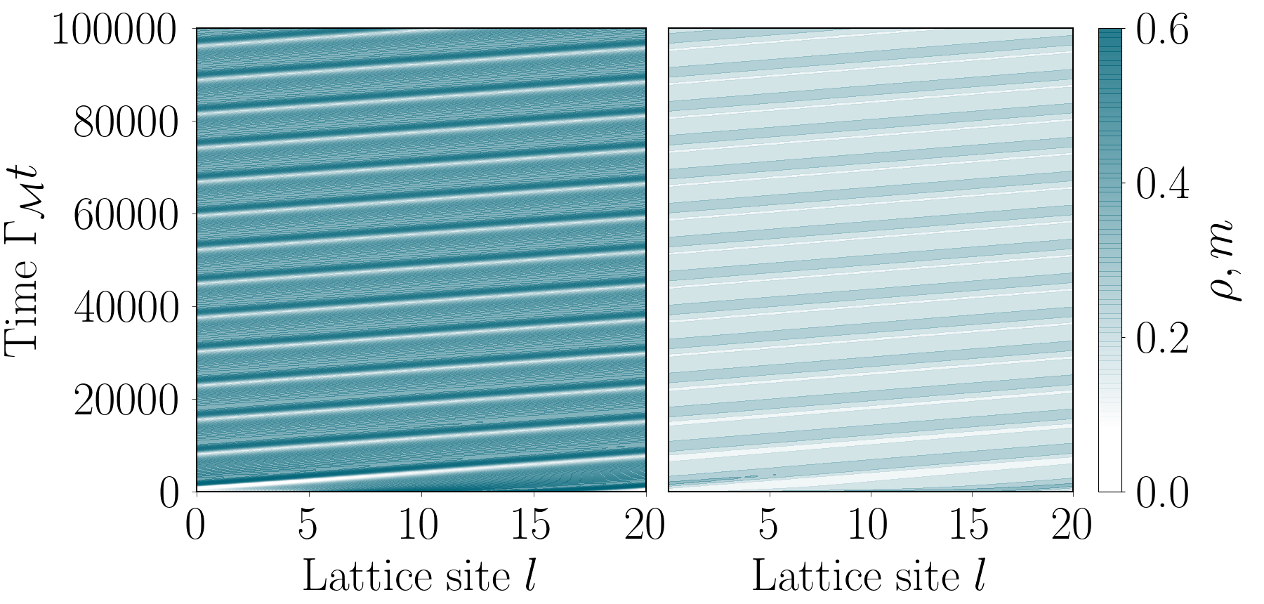
Extended Data Fig. 2: Traveling domain wall solutions. Dynamics of the density (left) and magnetization (right) for an initial cluster as a function of lattice site $l$ and time $t$ of the coarse-grained solution of the Lindblad-master equation obtained for parameters $L=20$, $K=4$, $\gamma_{\rho}=0.2$, $\gamma_{m}=0.6$, $\Gamma_{\mathcal{A}}/\Gamma_{\mathcal{M}}=0.1$

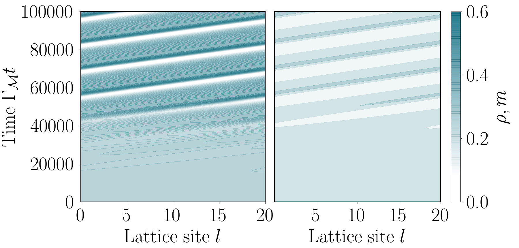
Extended Data Fig. 3: Emergence of traveling domain walls. Dynamics of the density (left) and magnetization profile (right) for an initial homogeneous state with weak noise. The homogeneous solution is unstable and traveling domain walls are formed after an initial transient regime. Simulations parameters: $L=20$, $K=4$, $\gamma_{\rho}=0.2$, $\gamma_{m}=0.6$, $\Gamma_{M}=1$, $\Gamma_{F}=0.1$.

Our numerical analysis of the coarse-grained description exhibits two main features. When $\Gamma_{\mathcal{M}}=\Gamma_{\mathcal{A}}$, as we have for the exact numerics in the main text, we find that the homogeneous solution is the attractor of the dynamics. Most importantly, however, we find that for $\Gamma_{\mathcal{M}}/\Gamma_{\mathcal{A}}=0.1$ also stable inhomogeneous solutions exist in the form of traveling ’domain walls’. In Extended Data Fig. 2 we consider an initial state where the system only contains $\uparrow$ particles and their density is distributed according to a Gaussian distribution $1/2\exp(-0.5((x-L/2)/\sigma)^{2})$ with $\sigma=0.5$. We observe that the initial cluster is stable in time with a persistent wave pattern visible in Extended Data Fig. 2. On top of this, we further find that in the considered regime the homogeneous solution actually becomes unstable, as we evidence in Extended Data Fig. 3. There, we consider an initial condition with a homogeneous magnetization and density, i.e., $\rho=m=0.25$, corresponding to a homogeneous flocking state of our quantum model, with a slight noise added on top of the homogeneous background. Concretely, we added to each site a uniformly distributed random number in $[-5\times 10^{-4},5\times 10^{-4}]$. We see that the system stays close to the homogeneous solution for some time, but eventually a traveling wave pattern emerges.

Data availability  
The data displayed in the figures is available on Zenodo Khasseh et al. .

Acknowledgements  
We acknowledge valuable discussions with Ricard Alert, Rainer Blatt, Juan Garrahan, Michael Knap, Igor Lesanovsky, Frank Pollmann, Achim Rosch, and Johannes Zeiher. This project has received funding from the European Research Council (ERC) under the European Union’s Horizon 2020 research and innovation programme (grant agreement No. 853443), and M. H. further acknowledges support by the Deutsche Forschungsgemeinschaft via the Gottfried Wilhelm Leibniz Prize program. Parts of the numerical simulations were performed at the Max Planck Computing and Data Facility in Garching.

SUPPLEMENTARY INFORMATION

I Classical analogue of the quantum flocking model

In order to further argue, that the quantum model studied in the main text exhibits a flocking phase, we study here for completeness a classical analogue. Concretely, we consider again a one-dimensional chain occupied by two species of particles $\sigma=\uparrow,\downarrow$. As for the quantum model, we assume an excluded volume for these particles in that a given lattice site cannot be occupied by two particles of the same type. The dissipative processes of the Lindblad master equation exhibit a straightforward classical analog. Concerning the hopping of particles, with a direction depending on their internal degrees of freedom $\sigma$, we consider jump probabilities $P_{\mathcal{M}_{l\uparrow}}=(n_{l\uparrow}+1)(n_{l+1\uparrow}-1)$ and $P_{\mathcal{M}_{l\downarrow}}=(n_{l+1\downarrow}+1)(n_{l\downarrow}-1)$. Here, $n_{l\sigma}$ denotes the occupation on lattice site $l$ with a particle of species $\sigma$ and $m_{l}=n_{l\uparrow}-n_{l\downarrow}$ the magnetization. As in the quantum case, this is the process which makes the particles active. Further, for the alignment process we define a jump probability $P_{{\cal A}_{l\sigma}}=\mathrm{exp}(-K/(2r){m}_{l}\sum_{|j|=1}^{r}{m}_{l+j})(n_{l\sigma}+1)(n_{l\bar{\sigma}}-1)$ with $K$ denoting the alignment parameter and $r$ defining the interaction radius, as in the quantum model. We solve the resulting classical dynamics numerically by means of a synchronous update algorithm as in Ref. Singh and Mishra

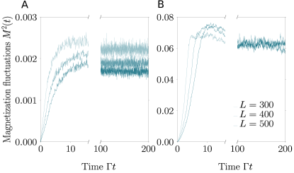
Fig. 1: Classical analogue of the quantum flocking problem. Dynamics of the magnetization fluctuations $M^{2}(t)$ for alignment parameter $K=0.5$ in A and $K=3.5$ in B.

Fig. 2: Quantum dynamics for alternative dynamical setups. A Dynamics of the Binder cumulant $U(t)$ for two types of initial product states, as indicated by the legend, converging to the same asymptotic steady state value. The numerical data has been obtained for a system size $L=8$, quantum amplitude $h/\Gamma=1/2$, and alignment parameter $K=3.8$. B Binder cumulant $U(t)$ obtained for two different unravelings of the Lindblad master equation and $h/\Gamma=0.2,2.0$ and $K=2.0$.

For the initial condition we choose a state with a vanishing magnetization in a specific configuration, where particles are placed on the chain in $\uparrow$-and-$\downarrow$ pairs, occupying a quarter of the chain’s $L$ sites and leaving the remaining part of the chain unoccupied. For a spin chain with L=8 sites, the initial state is given by $\{\uparrow\downarrow,\uparrow\downarrow,0,0,0,0,0,0\}$. In order to detect the long-range ordered flocking phase in the present classical model we study the order parameter fluctuations:

$$\langle M^{2}(t)\rangle=\frac{1}{L^{2}}\sum_{lj}\langle m_{l}(t)m_{j}(t)\rangle~{},$$ (26)

where $\langle...\rangle$ denotes the average over different trajectories, $m_{l}=n_{l\uparrow}-n_{l\downarrow}$, and $n_{l\uparrow(\downarrow)}$ represent the number of up(down) spins at site $l$. For a system with long-range order, we have that $M^{2}>0$ whereas for a disordered phase $M^{2}\to 0$ in the thermodynamic limit.

In Fig. 1, we show the numerically obtained evolution of $M^{2}$ for two different values of the alignment parameter, $K=0.5$ and $K=3.5$, as well as for different system sizes $L$. We observe that in both cases the order parameter eventually reaches a non-zero value in the long-time limit. Importantly, however, for $K=0.5$ the value of $M^{2}$ becomes smaller as the system size $L$ increases, whereas for $K=3.5$ we find that $M^{2}$ remains constant. This suggests that this classical model exhibits a flocking phase at sufficiently large values of the alignment parameter $K$.

II Alternative dissipative alignment processes

As discussed in the main text we have also explored alternative versions of dissipative alignment processes with quantum jump operators:

$$\quad\hat{\mathcal{A}}_{l\sigma}=\hat{c}^{\dagger}_{l\sigma}\hat{c}_{l\overline{\sigma}}\hat{P}_{l}\,,$$ (27)

by utilizing different variants of $\hat{P}_{l}$ leading to different kinds of conditional particle-flip processes. This includes:

1. $\hat{P}_{l}=\mathrm{exp}(-K/(2r)\hat{m}_{l}\sum_{|j|=1}^{r}\hat{m}_{l+j})$, which is utilized in the main text.

2. $\hat{P}_{l}=1-K/(2r)\hat{m}_{l}\sum_{|j|=1}^{r}\hat{m}_{l+j}$, which can be viewed as the linearized version of the previous one.

3. $\hat{P}_{l}=\sum_{\sigma}\hat{P}_{l\sigma}2^{-1}$ with $\hat{P}_{l\sigma}=\hat{m}_{l}(1+\sigma\hat{m}_{l})\delta(\sum_{|j|=1}^{r}\hat{m}_{l+j}+\sigma M_{0})$. This version induces jumps just when the surrounding magnetization $\sum_{|j|=1}^{r}\hat{m}_{l+j}$ matches precisely some predefined value $M_{0}$.

In Fig. 2, we show the numerical data obtained for all these three cases. As one can see, in all variants we find evidence for a quantum flocking phase. These numerical observations are consistent with the coarse-grained analysis of the Lindblad master equation in the main text, where in the end the sole role of the $\hat{P}_{l}$ operator is to provide some nonlinear terms in the magnetization in the respective Taylor expansion.

III Initial conditions

In this section, we aim to provide evidence that the emergence of quantum flocks in our model is not specific to the precise details of the initial condition. For that purpose, we show in Fig. 2 the dynamics corresponding to two initial states: $|\psi_{0}\rangle=\otimes_{l=1}^{N}|\psi_{0}\rangle_{l}\otimes_{l=N+1}^{L}\ket{0}_{l}$ with $|\psi_{0}\rangle_{l}=2^{-1/2}(\ket{\uparrow}_{l}+\ket{\downarrow}_{l})$ and $|\psi_{0}\rangle_{l}=\ket{\uparrow\downarrow}_{l}$.

In Fig. 2 we show the evolution of the Binder cumulant $U(t)$ for these two initial conditions for a system of size $L=8$, alignment parameter $K=3.8$ and quantum amplitude $h/\Gamma=1/2$. While the dynamics of the Binder cumulant differs on short times, as expected for different initial conditions, both time evolutions reach the same asymptotic long-time steady state value of $U(t)$.

IV Experimental Realization

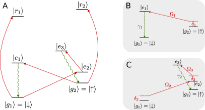
Fig. 3: Level scheme. Panel A shows the full level scheme of a Rydberg atom that can encode both particle species $\ket{\uparrow/\downarrow}$ in the states $\ket{g_{1/2}}$. These are coherently coupled to highly excited Rydberg states $\ket{r_{1/2}}$ to implement an alignment dynamics that is akin to the one used in the main text, exploiting the Rydberg blockade mechanism. Panel B and C show the dissipative spin flip processes through coherent coupling to excited states (red) that decay dissipatively (green).

In the following we discuss how the elementary building blocks of the quantum dynamics described in the main text may be realized in an experimental setup. We consider the directed motion induced by the quantum jump operators $\mathcal{M}_{l\sigma}$ separately from the alignment dynamics $\mathcal{A}_{l\sigma}$.  
Directed Motion. In order to realize the directed motion, we take as the starting point a $U(1)$ lattice gauge theory in the form of a so-called quantum link model Chandrasekharan and Wiese (1997); Bañuls et al. (2020). Concretely, we consider matter coupled to a spin-$1/2$ gauge degree of freedom on the link with a minimal coupling. For a single bond this reduces to the following Hamiltonian Chandrasekharan and Wiese (1997); Bañuls et al. (2020):

$$H=\omega(c_{1}^{\dagger}S^{+}c_{2}+\mathrm{h.c.})$$ (28)

with $\omega$ denoting the amplitude of that process. Here, $S^{+}$ and $S^{-}$ are the usual spin-$1/2$ ladder operators and $c_{1/2}$ denote some annihilation operators. In analogy to the model in the main text we consider hard-core bosons. In the following, we will introduce an abbreviation $B^{\dagger}=c_{1}^{\dagger}c_{2}$ so that we work with the general Hamiltonian:

$$H=\omega(S^{+}B^{\dagger}+S^{-}B)\ .$$ (29)

In order to generate the dissipative directed motion we subject this Hamiltonian to additional fast dissipative dynamics in the form of a decay of the gauge degree of freedom. This corresponds to a Lindblad master equation of the form:

$$\frac{d\rho}{dt}=-i[H,\rho]+\gamma S^{-}\rho S^{+}-\frac{\gamma}{2}\{S^{+}S^{-},\rho\}\,,$$ (30)

with $\gamma$ the rate of the decay process, which we will choose as $\gamma\gg\omega$. The underlying mechanism is that the fast spin decay ensures that - although the interaction Hamiltonian is Hermitian - the process $S^{+}B^{\dagger}$ is favored by the dissipative system as compared to $BS^{-}$. We proceed to adiabatically eliminate the fast dynamics related to the spin decay. To this end, we follow the construction shown in Ref. Mirrahimi and Rouchon (2009) but we note that in Ref. Mirrahimi and Rouchon (2009) an internal degree of freedom is eliminated and here we eliminate an external degree of freedom. We thus consider the projector $P=\ket{\uparrow}\bra{\uparrow}\otimes\mathds{1}$ and find the altered Hamiltonian

$$\bar{H}=(\mathds{1}-P)H(\mathds{1}-P)=0.$$ (31)

The quantum jump operator $Q=S^{-}\otimes\mathds{1}$ is altered as

$$\bar{\Gamma}\bar{Q}=(\mathds{1}-P)QH(\mathds{1}-P)=\omega\ket{\downarrow}\bra{\downarrow}B^{\dagger}$$ (32)

with $\bar{\Gamma}=\epsilon\gamma$. The slow dynamics described by the slow component $\varrho_{s}=(\mathds{1}-P)\rho(\mathds{1}-P)+Q\rho Q^{\dagger}$ of the full density matrix $\rho$ is hence revealed to follow the Lindblad master equation

$$\frac{d\varrho_{s}}{dt}= 2\frac{\omega^{2}}{\gamma}\left(2\ket{\downarrow}\bra{\downarrow}B^{\dagger}\varrho_{s}\ket{\downarrow}\bra{\downarrow}B-\right.$$

$$\left.-\ket{\downarrow}\bra{\downarrow}BB^{\dagger}\varrho_{s}-\varrho_{s}\ket{\downarrow}\bra{\downarrow}BB^{\dagger}\right)$$ (33)

Finally, we take the partial trace over the spin $1/2$ degree of freedom, i.e., $\varrho=\operatorname{tr}_{1/2}\varrho_{s}$ and we obtain the Lindblad master equation

$$\frac{d\varrho}{dt}=\frac{2\omega^{2}}{\gamma}\left(2B^{\dagger}\varrho B-BB^{\dagger}-\varrho BB^{\dagger}\right)$$ (34)

Recalling that $B^{\dagger}=c_{1}^{\dagger}c_{2}$ we find that this effective dynamics is exactly of the form of the directed motion used in our model in the main text.

Here, we have discussed an experimental realization for a single bond. The extension to a full chain is straightforward by starting with a lattice gauge theory on that chain and imposing strong independent decay channels for all the gauge spins. For the final realization of the directed motion in the considered quantum model, it would furthermore be necessary to implement the described dynamical process for two types of particles leading to the two-species scenario studied in the main text.

Alignment dynamics. In a next step we discuss how a the alignment process for the quantum flock might be realized in a system of Rydberg atoms. For that purpose we again consider just a single building block consisting of one atom with two internal states $\uparrow$ and $\downarrow$, for which we implement an effective dissipative spin-flip conditioned on an environment.

Fig. 3 illustrates the level scheme we consider to realize the alignment dynamics. The up to down flip ($\ket{\uparrow}\to\ket{\downarrow}$) in particular is highlighted in Fig. 3B. The three-level system involved in this transition is described by the density matrix $\rho$ that follows the Lindblad master equation

$$\frac{d\rho}{dt}=-i[H_{1},\rho]+\gamma_{1}\left(2L\rho L^{\dagger}-L^{\dagger}L\rho-\rho L^{\dagger}L\right)$$ (35)

with the quantum jump operator $L=\ket{g_{1}}\bra{e_{1}}$ modelling the dissipative $\ket{e_{1}}\to\ket{g_{1}}$ transition and the Hamiltonian $H_{1}=\delta_{1}\ket{g_{2}}\bra{g_{2}}+\Omega_{1}\ket{g_{2}}\bra{e_{1}}+\Omega_{1}^{*}\ket{e_{1}}\bra{g_{2}}$ describing the coherent driving of the $\ket{g_{2}}\to\ket{e_{1}}$ transition. For $\gamma_{1}\gg|\delta_{1}|,|\Omega_{1}|$ we may adiabatically eliminate the state $\ket{e_{1}}$ following, e.g., Ref. Mirrahimi and Rouchon (2009). The effective Hamiltonian of the reduced system is thus given by

$$H_{1}^{\rm(eff)}=(\mathds{1}-\ket{e_{1}}\bra{e_{1}})H_{1}(\mathds{1}-\ket{e_{1}}\bra{e_{1}})=\delta_{1}\ket{g_{2}}\bra{g_{2}}$$ (36)

and the effective quantum jump operator $L^{\rm(eff)}$ reads

$$L^{\rm(eff)}=\frac{1}{\gamma_{1}}(\mathds{1}-\ket{e_{1}}\bra{e_{1}})LH(\mathds{1}-\ket{e_{1}}\bra{e_{1}})=\frac{\Omega^{*}}{\gamma_{1}}\ket{g_{1}}\bra{g_{2}}$$ (37)

Writing $\sigma^{-}=\ket{g_{1}}\bra{g_{2}}$ and $\sigma^{+}=(\sigma^{-})^{\dagger}$ we find the effective Lindblad master equation by simply replacing $H_{1}\to H_{1}^{\rm(eff)}$ and $L\to L^{\rm(eff)}$ in the original Lindblad equation, viz.,

$$\frac{d\varrho_{s}}{dt}= -i[H_{1}^{\rm(eff)},\rho_{s}]+$$

$$+2\frac{|\Omega_{1}|^{2}}{\gamma_{1}}\left(2\sigma^{-}\rho\sigma^{+}-\sigma^{+}\sigma^{-}\rho-\rho\sigma^{+}\sigma^{-}\right)$$ (38)

Similarly, we may proceed for the down to up flip ($\ket{\downarrow}\to\ket{\uparrow}$) illustrated in Fig. 3C. Here, we need to eliminate the excited states $\ket{e_{2}}$ and $\ket{e_{3}}$. We observe that the state $\ket{g_{2}}$ does not couple coherently to the remainder of the system. Hence, the remainder forms a subsystem reminiscent to a standard Lambda system, only that the coherently coupled state is in the middle of the spectrum. This detail merely reverses the sign of a single detuning such that the Hamiltonian may be written as

$$H_{2}=\delta_{2}\ket{g_{1}}\bra{g_{1}}-\delta_{3}\ket{e_{3}}\bra{e_{3}}+\Omega_{2}\ket{g_{1}}\bra{e_{2}}+$$

$$+\Omega_{2}\ket{e_{2}}\bra{g_{1}}+\Omega_{3}\ket{e_{2}}\bra{e_{3}}+\Omega_{3}^{*}\ket{e_{3}}\bra{e_{2}}$$ (39)

The Lindblad equation dissipatively coupling the state $\ket{g_{2}}$ then reads

$$\frac{d\rho}{dt}=-i[H,\rho]+\frac{\gamma_{2}}{2}\left(2L\rho L^{\dagger}-L^{\dagger}L\rho-\rho L^{\dagger}L\right)$$ (40)

with the quantum jump operator $L=\ket{g_{2}}\bra{e_{3}}$. Now, we first eliminate the state $\ket{e_{3}}$ for $\gamma_{2}\gg|\Omega_{3}|,|\delta_{3}|$ similar to the opposite spin flip discussed above. This yields a new damping constant $\gamma^{\prime}=2|\Omega_{3}|^{2}/\gamma_{2}$ and for $\gamma^{\prime}\gg|\Omega_{2}|,|\delta_{2}|$ we may adiabatically eliminate the state $\ket{e_{2}}$. The elimination condition is generally met since $|\Omega_{2}|\ll\gamma^{\prime}\sim|\Omega_{3}|^{2}/\gamma_{2}\ll\gamma_{2}$. This procedure yields the effective Lindbladian

$$\frac{d\tilde{\varrho}_{s}}{dt}= -i[H_{2}^{\rm(eff)},\tilde{\rho}_{s}]+$$

$$+ \frac{|\Omega_{2}|^{2}}{|\Omega_{3}|^{2}}\gamma_{2}\left(2\sigma^{-}\rho\sigma^{+}-\sigma^{+}\sigma^{-}\rho-\rho\sigma^{+}\sigma^{-}\right)$$ (41)

with the effective Hamiltonian

$$H_{2}^{\rm(eff)}=\delta_{2}\ket{g_{1}}\bra{g_{1}}.$$ (42)

Rydberg dressing. Having established the dynamics to induce dissipative spin flips in ultracold atoms we now need to introduce a mechanism that is capable to (de)activate the spin flips depending on the surrounding magnetization, which would effectively realize the alignment process 3 discussed in the Supplement Sec. II. To achieve this we dress both spin states respectively with a Rydberg state $\ket{r_{1/2}}$, see Fig. 3. The key impact of this Rydberg dressing is to shift the energy levels $\delta_{1}$ and $\delta_{2}$ corresponding to the states $|\uparrow\rangle$ and $|\downarrow\rangle$ depending on the presence of other atoms. Consider for instance a situation where only for a specific environment $\delta_{1}=\delta_{2}=0$, leading to the desired dissipative spin flip. Additionally, let’s assume that for any other environment $\delta_{1/2}\gg\gamma_{1/2}$, thus we can effectively neglect the dissipative process. Summarizing:

• the Rydberg dressing of $\ket{\downarrow}$ with $\ket{r_{1}}$ switches the $\ket{\downarrow}\to\ket{\uparrow}$ transition on/off.

• the Rydberg dressing of $\ket{\uparrow}$ with $\ket{r_{2}}$ switches the $\ket{\uparrow}\to\ket{\downarrow}$ transition on/off.

References

- Gross and Bloch (2017) C. Gross and I. Bloch, Science 357, 995 (2017).
- Monroe et al. (2021) C. Monroe, W. C. Campbell, L. M. Duan, Z. X. Gong, A. V. Gorshkov, P. W. Hess, R. Islam, K. Kim, N. M. Linke, G. Pagano, P. Richerme, C. Senko, and N. Y. Yao, Rev. Mod. Phys. 93, 025001 (2021).
- Browaeys and Lahaye (2020) A. Browaeys and T. Lahaye, Nature Phys. 16, 132 (2020).
- Blais et al. (2021) A. Blais, A. L. Grimsmo, S. M. Girvin, and A. Wallraff, Rev. Mod. Phys. 93, 025005 (2021).
- Schreiber et al. (2015) M. Schreiber, S. S. Hodgman, P. Bordia, H. P. Lüschen, M. H. Fischer, R. Vosk, E. Altman, U. Schneider, and I. Bloch, Science 349, 842 (2015).
- Smith et al. (2016) J. Smith, A. Lee, P. Richerme, B. Neyenhuis, P. W. Hess, P. Hauke, M. Heyl, D. A. Huse, and C. Monroe, Nature Phys. 12, 907 (2016).
- Choi et al. (2017) S. Choi, J. Choi, R. Landig, G. Kucsko, H. Zhou, J. Isoya, F. Jelezko, S. Onoda, H. Sumiya, V. Khemani, C. von Keyserlingk, N. Y. Yao, E. Demler, and M. D. Lukin, Nature (London) 543, 221 (2017).
- Zhang et al. (2017) J. Zhang, P. W. Hess, A. Kyprianidis, P. Becker, A. Lee, J. Smith, G. Pagano, I. D. Potirniche, A. C. Potter, A. Vishwanath, N. Y. Yao, and C. Monroe, Nature (London) 543, 217 (2017).
- Bernien et al. (2017) H. Bernien, S. Schwartz, A. Keesling, H. Levine, A. Omran, H. Pichler, S. Choi, A. S. Zibrov, M. Endres, M. Greiner, V. Vuletić, and M. D. Lukin, Nature (London) 551, 579 (2017).
- Jülicher et al. (1997) F. Jülicher, A. Ajdari, and J. Prost, Rev. Mod. Phys. 69, 1269 (1997).
- Ramaswamy (2010) S. Ramaswamy, Annu. Rev. Condens. Matter Phys. 1, 323 (2010).
- Marchetti et al. (2013) M. C. Marchetti, J.-F. Joanny, S. Ramaswamy, T. B. Liverpool, J. Prost, M. Rao, and R. A. Simha, Rev. Mod. Phys. 85, 1143 (2013).
- Prost et al. (2015) J. Prost, F. Jülicher, and J.-F. Joanny, Nature Phys. 11, 111 (2015).
- Cates and Tjhung (2018) M. E. Cates and E. Tjhung, J. Fluid Mech. 836, P1 (2018).
- Weber et al. (2019) C. A. Weber, D. Zwicker, F. Jülicher, and C. F. Lee, Rep. Prog. Phys. 82, 064601 (2019).
- Vicsek et al. (1995) T. Vicsek, A. Czirók, E. Ben-Jacob, I. Cohen, and O. Shochet, Phys. Rev. Lett. 75, 1226 (1995).
- Toner et al. (2005) J. Toner, Y. Tu, and S. Ramaswamy, Annals of Physics 318, 170 (2005).
- Chaté (2020) H. Chaté, Annu. Rev. Condens. Matter Phys. 11, 189 (2020).
- Solon and Tailleur (2013) A. P. Solon and J. Tailleur, Phys. Rev. Lett. 111, 078101 (2013).
- Solon and Tailleur (2015) A. P. Solon and J. Tailleur, Phys. Rev. E 92, 042119 (2015).
- Weber et al. (2014) C. A. Weber, C. Bock, and E. Frey, Phys. Rev. Lett. 112, 168301 (2014).
- Fodor et al. (2022) É. Fodor, R. L. Jack, and M. E. Cates, Annu. Rev. Condens. Matter Phys. 13, 215 (2022).
- Bär et al. (2020) M. Bär, R. Großmann, S. Heidenreich, and F. Peruani, Annu. Rev. Condens. Matter Phys. 11, 441 (2020).
- Gardiner and Zoller (2004) C. Gardiner and P. Zoller, Quantum noise: a handbook of Markovian and non-Markovian quantum stochastic methods with applications to quantum optics (Springer Science & Business Media, 2004).
- (25) Y. Zheng and H. Löwen, arXiv:2305.16131 .
- (26) M. Yamagishi, N. Hatano, and H. Obuse, arXiv:2305.15319 .
- Streltsov et al. (2017) A. Streltsov, G. Adesso, and M. B. Plenio, Rev. Mod. Phys. 89, 041003 (2017).
- Rodriguez and Laio (2014) A. Rodriguez and A. Laio, Science 344, 1492 (2014).
- Czirók et al. (1999) A. Czirók, A.-L. Barabási, and T. Vicsek, Phys. Rev. Lett. 82, 209 (1999).
- O’Loan and Evans (1999) O. O’Loan and M. Evans, J. Phys. A Math. Gen. 32, L99 (1999).
- Bertin et al. (2009) E. Bertin, M. Droz, and G. Grégoire, J. Phys. A: Math. Theor. 42, 445001 (2009).
- Weber et al. (2013) C. A. Weber, F. Thüroff, and E. Frey, New J. Phys. 15, 045014 (2013).
- Thüroff et al. (2014) F. Thüroff, C. A. Weber, and E. Frey, Phys. Rev. X. 4, 041030 (2014).
- Chaté et al. (2008) H. Chaté, F. Ginelli, G. Grégoire, and F. Raynaud, Phys. Rev. E. 77, 046113 (2008).
- Benvegnen et al. (2022) B. Benvegnen, H. Chaté, P. L. Krapivsky, J. Tailleur, and A. Solon, Phys. Rev. E. 106, 054608 (2022).
- Weber et al. (2012) C. A. Weber, V. Schaller, A. R. Bausch, and E. Frey, Phys. Rev. E. 86, 030901 (2012).
- Orús (2019) R. Orús, Nature Rev. Phys. 1, 538 (2019).
- Carleo and Troyer (2017) G. Carleo and M. Troyer, Science 355, 602 (2017).
- Schmitt and Heyl (2020) M. Schmitt and M. Heyl, Phys. Rev. Lett. 125, 100503 (2020).
- Cates and Tailleur (2015) M. E. Cates and J. Tailleur, Annu. Rev. Condens. Matter Phys. 6, 219 (2015).
- Giomi (2015) L. Giomi, Phys. Rev. X 5, 031003 (2015).
- Huepe and Aldana (2004) C. Huepe and M. Aldana, Phys. Rev. Lett. 92, 168701 (2004).
- Cavagna et al. (2013) A. Cavagna, I. Giardina, and F. Ginelli, Phy. Rev. Lett. 110, 168107 (2013).
- Gómez-Nava et al. (2022) L. Gómez-Nava, R. Bon, and F. Peruani, Nature Phys. 18, 1494 (2022).
- Schaller (2014) G. Schaller, Open quantum systems far from equilibrium, Vol. 881 (Springer, 2014).
- Schütz (2003) G. M. Schütz, J. Phys. A: Math. Gen. 36, R339 (2003).
- (47) R. Khasseh, S. Wald, R. Moessner, C. A. Weber, and M. Heyl, 10.5281/zenodo.8208685.
- (48) R. Singh and S. Mishra, arXiv:1704.04041 .
- Chandrasekharan and Wiese (1997) S. Chandrasekharan and U. J. Wiese, Nucl. Phys. B. 492, 455 (1997).
- Bañuls et al. (2020) M. C. Bañuls, R. Blatt, J. Catani, A. Celi, J. I. Cirac, M. Dalmonte, L. Fallani, K. Jansen, M. Lewenstein, S. Montangero, C. A. Muschik, B. Reznik, E. Rico, L. Tagliacozzo, K. Van Acoleyen, F. Verstraete, U.-J. Wiese, M. Wingate, J. Zakrzewski, and P. Zoller, Eur. Phys. J. D. 74, 165 (2020).
- Mirrahimi and Rouchon (2009) M. Mirrahimi and P. Rouchon, IEEE Trans. Autom. Control. 54, 1325 (2009).