Defining a quantum active particle using a non-unitary quantum walk

Abstract

The main aim of the present paper is to define an active matter in a quantum framework and investigate difference and commonalities of quantum and classical active matters. Although the research field of active matter has been expanding wider and wider, most research is conducted in classical systems. We here propose a truly deterministic quantum active-matter model with a non-unitary quantum walk as minimal models of quantum active matter in one- and two-dimensional systems. We aim to reproduce similar results that Schweitzer et al. [Schweitzer98] obtained with their classical active Brownian particle; that is, the Brownian particle, with a finite energy take-up, becomes active and climbs up a potential wall. We realize such a system with non-unitary quantum walks. We introduce new internal states, the ground state $\ket{\mathrm{G}}$ and the excited state $\ket{\mathrm{E}}$, and a new non-unitary operator $N(g)$ for an asymmetric transition between $\ket{\mathrm{G}}$ and $\ket{\mathrm{E}}$. The non-Hermiticity parameter $g$ promotes transition to the excited state and hence the particle takes up energy from the environment. We realize a system without momentum conservation by manipulating a parameter $\theta$ for the coin operator for a discrete-time quantum walk; we utilize the property that the continuum limit of a one-dimensional discrete-time quantum walk gives the Dirac equation with its mass proportional to the parameter $\theta$ [Strauch06]. With our quantum active particle, we successfully observe that the movement of the quantum walker becomes more active in a non-trivial way as we increase the non-Hermiticity parameter $g$, which is similar to the classical active Brownian particle [Schweitzer98]. Meanwhile, we also observe three unique features of quantum walks, namely, ballistic propagation of peaks in one dimension, the walker staying on the constant energy plane in two dimensions, and oscillations originating from the resonant transition between the ground state $\ket{\mathrm{G}}$ and excited state $\ket{\mathrm{E}}$ both in one and two dimensions.

I Introduction

Active matter is a self-driven component or a collection of such components [Pismen21]. Active matter can be un-living matters as well as living ones like birds and fish. From a physical point of view, an active matter takes up energy from the environment, stores it inside, converts the internal energy into kinetic energy, and thereby moves (Fig. 1). The active Brownian particle [Romanczuk12], which appears in the following sections, is a prototypical example of active matter.

Figure 1: Schematic views of active matter. (a) A component that takes up energy from the environment, stores it inside, converts the stored internal energy to the kinetic energy and moves, or (b) an interacting collection of such components.

The research area of active matter is highly interdisciplinary; it extends over biology [Popkin16, Needleman17], chemistry [Doostmohammadi18], and physics [Gompper20]. Introduction of the idea of active matter enabled us to unify a variety of studies which had been investigated separately before and to understand their commonalities and universalities [Ohta15]. Starting from the models proposed by Vicsek [Vicsek95] and Toner and Tu [Toner95] separately in 1995, theoretical studies have lead the research of classical active matter. Various phenomena unique to active matter have been found, e.g. true long-range order [Vicsek95], giant number fluctuation (GNF) [Toner98, Chate08] and motility-induced phase separation (MIPS) [Cates13, Cates15]. A recent research [Sone20] connecting classical active matter and topological phenomena, such as the Hall effect, is gathering much attention. These studies have attracted and fascinated many researchers, and now that more and more models are realized in experiments [Narayan07, Zhang10, Redner13, Kawaguchi17, Nishiguchi18], the research field has been expanding wider and wider.

However, most research is conducted in classical systems. There are few works that tried to introduce the concept of active matter into quantum systems. Adachi et al. [Adachi22] modeled a many-body version of quantum active matter, connecting a classical stochastic active matter to a non-Hermitian quantum spin systems, which they referred to a “stoquastic” Hamiltonian; Zheng and Löwen [Zheng23] used a quantum harmonic oscillator with its potential minima externally driven by stochastic active dynamics. The authors of the former paper recently considered another model in one dimension [Takasan23] based on their first model [Adachi22], finding a flocking phase as ferromagnetism of a quantum spin model. There is recently another work on active quantum flocks [Khasseh23] by Khasseh et al.

In the present paper, we define a quantum active matter using discrete-time quantum walks[Aharonov93, Meyer96, Farhi98, Ambainis12, Asaka21]. Since the quantum walk does not have any stochasticity of classical random walks and does not have any classical limits, neither does our model.

Table 1: Classification of systems without energy conservation. Studying quantum active matter enables us to extend non-Hermitian physics to systems without momentum conservation and to extend classical active matter to quantum systems.

We have in our mind the diagram shown in Table 1. We believe that the following two points are essential properties for a system to be an active matter:

1. neither energy nor momentum are conserved;

2. the kinetic motion depends on particles’ internal states.

The energy non-conservation results in temporally inhomogeneous dynamics, such as decay and growth, whereas the momentum non-conservation, which is equivalent to the breakdown of the law of action and reaction, results in spatially inhomogeneous dynamics, such as a pair of birds meeting up and flying along together. We would define distinctive universality classes of quantum active matter by updating non-Hermitian, energy non-conservative quantum models into the new realm of momentum non-conservation.

In this paper, trying to find a minimal model of quantum active matter, we define a one-particle non-Hermitian quantum system that exhibits real-time evolution in a fully quantum range without external manipulation as in Ref. [Zheng23]. In our quantum active-matter model, internal states that are strongly correlated with the environment dominate the system dynamics. Strong correlation with the environment makes the system open and non-Hermitian, without energy conservation. We note that the non-Hermiticity of our model Hamiltonian belongs to the class of so-called pseudo-Hermiticity [Mostafazadeh02-1, Mostafazadeh02-2, Mostafazadeh02-3], because of which all energy-like eigenvalues of the unitary dynamics are real, although the energy expectation values are not conserved. It never exhibits Markovian decays due to complex eigenvalues of non-Hermitian Hamiltonians that one would find in the Gorini-Kosakowski-Sudarshan-Lindblad equation [GKS76, Lindblad76] under postselection of no quantum jumps [Ott16, Ashida16, Ashida17, Ashida20, Nakagawa20, Joglekar19, Joglekar21]. One notable point of our model is that we break the momentum conservation deliberately. Hence our system evolves differently from the cases of ordinary non-Hermitian quantum mechanics.

I.1 Classical active Brownian Particle

Let us next review a previous research on a prototypical classical active Brownian particle [Schweitzer98]. This model may differ from major ones in the context of studies on active matter [Geier05, Howse07, Paxton04]. However, the authors of the study that we review here made the correspondence between the internal energy of the particle and its dynamics very clearly, which is why we chose this study to start with. Schweitzer et al. [Schweitzer98] studied the dynamics of a Brownian particle with ability to take up energy from the environment, store it inside, convert the internal energy into kinetic energy and move. In order to model the dynamics, they added a new term of the internal energy $e(t)$ to the right-hand side of the Langevin equation. They first studied dynamics of an active Brownian particle under a harmonic potential with a constant energy take-up. The active Brownian particle moved almost on a limit cycle with a finite energy take-up, whereas a simple Brownian particle without an energy take-up did not. We aim to reproduce similar results to theirs: a quantum particle moves around more actively, climbing up the harmonic potential with a finite energy take-up. At the same time, we aim to observe its quantum features not present in its classical counterpart. In order to achieve them, we use non-unitary quantum walks[Mochizuki16, Xiao17, Hatano21b] as a tool.

I.2 Quantum walks

The quantum walk is a quantum analogue of random walk. Nonetheless, note that the quantum walk exhibits distinctively quantum dynamics, without any stochasticity. Instead of stochastic fluctuations of the classical random walker, the quantum walker moves under quantum interference at each site, which deterministically governs the dynamics of the walker’s wave function. Its classical limit might be possible only after introducing decoherence or other additional effects.

Quantum walk was originally introduced by Aharonov et al. [Aharonov93], who first referred to it as “quantum random walk”. Meyer [Meyer96] built a systematic model and found a correspondence to Feynman’s path integral [Feynman65] of the Dirac equation. Started by Farhi and Gutmann [Farhi98], quantum walks have been well studied in the context of quantum information [Ambainis12, Asaka21]. To this day, studies of quantum walks have become even more interdisciplinary and extended over a variety of research fields, such as biophysics [Engel07, Dudhe22] and condensed-matter physics [Oka05], particularly topological materials [Kitagawa10, Obuse11, Kitagawa12, Asboth13].

There are two types of time evolution: continuum-time quantum walks and discrete-time quantum walks. In the present paper, we focus on the latter, in which the space and time are both discrete. In Sec. II, we first investigate non-unitary quantum walk as a quantum active particle in one dimension. In need of extension of our quantum active matter to higher dimensions, we utilize in Sec. LABEL:sec3 multi-dimensional quantum walks [Yamagishi23] with which we can make correspondence to the Dirac equation and further to the Schrödinger equation in higher dimensions. Section. LABEL:sec4 summarizes the paper. To make the paper self-contained, we provide a compact review of the quantum walk in Appendix LABEL:appQW.

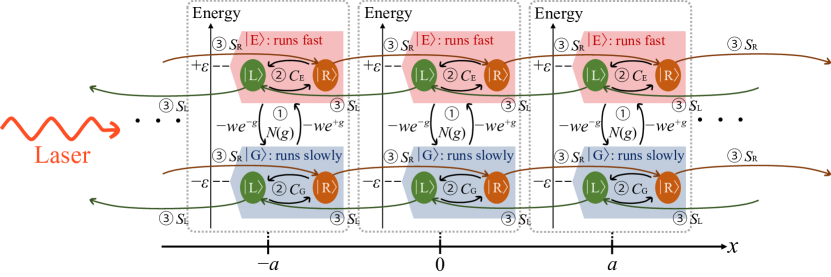
Figure 2: Time evolution of our quantum active particle in one dimension. There are four internal states, namely, $(\ket{\mathrm{L}}\oplus\ket{\mathrm{R}})\otimes(\ket{\mathrm{G}}\oplus\ket{\mathrm{E}})$ at each site. The parameters $\varepsilon$, $w$ and $g$ are all real. We have the coin operator (\scriptsize{2}⃝), the shift operator (\scriptsize{3}⃝), and the new operator for asymmetric transition between the ground state $\ket{\mathrm{G}}$ and the excited state $\ket{\mathrm{E}}$, which describes energy take-up (\scriptsize{1}⃝). We use different $\theta$ for the ground state $\ket{\mathrm{G}}$ and the excited state $\ket{\mathrm{E}}$ to realize a system without momentum conservation.

II Quantum active particle in one dimension

II.1 One-dimensional model

In one dimension, our quantum active particle has four internal states in total, namely, $(\ket{\mathrm{L}}\oplus\ket{\mathrm{R}})\otimes(\ket{\mathrm{G}}\oplus\ket{\mathrm{E}})$. Here, $\ket{\mathrm{L}}$ and $\ket{\mathrm{R}}$ denote the leftward and rightward states, respectively, while $\ket{\mathrm{G}}$ and $\ket{\mathrm{E}}$ denote the ground and excited states, respectively. We define the time evolution of our one-dimensional quantum active particle $\ket{\psi(T)}=[{U^{(1)}(g)}]^{T}\ket{\psi(0)}$ for $T\in\mathbb{Z}$ in terms of the following operators:

$$N^{(1)}(g) :=\sum_{x}\quantity[\outerproduct{x}{x}\otimes\mathrm{e}^{-\mathrm{i}H_{\mathrm{NH}}^{(1)}(g)}],$$ (1)

$$C^{(1)} :=\sum_{x}\quantity[\outerproduct{x}{x}\otimes\mathrm{e}^{-\mathrm{i}H_{C}^{(1)}(x)}],$$ (2)

$$S^{(1)} :=\sum_{x}\quantity[\outerproduct{x-a}{x}\otimes\outerproduct{\mathrm{L}}{\mathrm{L}}+\outerproduct{x+a}{x}\otimes\outerproduct{\mathrm{R}}{\mathrm{R}}],$$ (3)

with $U^{(1)}(g):=SCN^{(1)}(g)$ and with the lattice constant $a$. Here,

We used the bases $\{\ket{\mathrm{L}}\otimes\ket{\mathrm{G}},\ket{\mathrm{R}}\otimes\ket{\mathrm{G}},\ket{\mathrm{L}}\otimes\ket{\mathrm{E}},\ket{\mathrm{R}}\otimes\ket{\mathrm{E}}\}$ in this order to represent the matrices. In Eq. (II.1), $\mp\varepsilon$ denotes the levels of $\ket{\mathrm{G}}$ and $\ket{\mathrm{E}}$, respectively, while the non-Hermitian parameter $g$ specifies the difference in the transitions between the two levels. The non-Hermiticity of $H_{\mathrm{NH}}^{(1)}$ makes the total time-evolution operator $U^{(1)}(g)$ non-unitary. We can interpret the non-Hermiticity of $H_{\mathrm{NH}}^{(1)}$ as an effect of laser pumping; see Sec. LABEL:sec2.2. Note that the energy conservation is broken because of our non-Hermitian Hamiltonian $H_{\mathrm{NH}}^{(1)}(g)$. Thus it satisfies the first half of the property (i) of quantum active matter; the energy is not conserved. In fact, we will show below in Eq. (II.1) that the Hamiltonian (II.1) has a symmetry called the pseudo-Hermiticity [Mostafazadeh02-1, Mostafazadeh02-2, Mostafazadeh02-3], and hence the energy eigenvalues remain real, not depending on $g$ at all, but the energy expectation value are not conserved.

In Eq. (II.1), we set the parameter for the excited state $\theta_{\mathrm{E}}(x)$ generally less than that of the ground state $\theta_{\mathrm{G}}(x)$. This is because of the following reason. The continuum limit of the unitary time evolution of one-dimensional [Strauch06] and two-dimensional [Yamagishi23] quantum walks yields a Dirac Hamiltonian with the parameters for the coin operator $\theta$ of the former being proportional to the mass terms of the latter. We set $\theta_{\mathrm{E}}<\theta_{\mathrm{G}}$ so that we can make our quantum active particle run faster in the excited state than in the ground state. In other words, our active quantum walker does not conserve the momentum, which is the second half of the property (i) of quantum active matter; the momentum is not conserved either. Since it runs faster when pumped from the ground state to the excited state, it also satisfies the property (ii) of quantum active matter; the kinetic motion depends on particles’ internal states. See Fig. 2 for details of the time evolution.

One notable point is that we can make the non-Hermitian matrix $H_{\mathrm{NH}}^{(1)}(g)$ Hermitian with a similarity transformation called the imaginary gauge transformation [Hatano96, Hatano97]

$$A(g)=\mathop{\mathrm{diag}}(\mathrm{e}^{-g/2},\mathrm{e}^{-g/2},\mathrm{e}^{+g/2},\mathrm{e}^{+g/2})$$ (12)

as in

Inotherwords,theeigenvaluesofourHamiltonian(

II.1)remainrealforanyvalueso